


Introduction
Hydrocarbon production is known to induce fault reactivation and seismic events due to fluid pressure reduction at depth (Baranova et al., Reference Baranova, Mustaqeem and Bell1999; McGarr et al., Reference McGarr, Simpson, Seeber and Lee2002; Suckale, Reference Suckale2009). This process is observed for example in the Groningen area of the Netherlands, where natural gas is produced from Rotliegend reservoirs covered by thick Zechstein salt layers (van Thienen-Visser & Breunese, Reference van Thienen-Visser and Breunese2015; van Thienen-Visser et al., Reference van Thienen-Visser, Pruiksma and Breunese2015). In brittle faults, this process is thought to be independent of the long-term rate of loading. Rock salt rheology, however, has a viscous component (Urai et al. Reference Urai, Schléder, Spiers, Kukla, Littke, Bayer, Gajewski, Brink and Winter2008). Roest & Kuilman (Reference Roest and Kuilman1994) suggest that salt may locally intrude downward along a fault plane and affect seismicity. If in the Groningen area there is salt present in fault zones this may introduce a rate dependency to fault movement and change the magnitude distribution of seismic events. If and how salt can flow downwards into dilatant faults and how salt is distributed in fault zones is unexplored so far, and little is known of the possible effect of salt in faults on the frequency and magnitude of seismic events. We note here that there are many other fault zone processes which likely play a role here, such as fault healing and rate-and-state friction (e.g. Marone, Reference Marone1998), but these are not considered here.
Two conditions must be met to allow for salt entering a fault. First, the rocks underlying the salt must fail in extension or hybrid failure to form open voids. This requires a cohesive rock failing at small differential stresses, that is, small overburden thickness (Ferrill & Morris, Reference Ferrill and Morris2003; Ferrill et al., Reference Ferrill, Wyrick, Morris, Sims and Franklin2004, Reference Ferrill, McGinnis, Morris and Smart2012; Chemenda et al., Reference Chemenda, Nguyen, Petit and Ambre2011; Nguyen et al., Reference Nguyen, Chemenda and Ambre2011; Abdelmalak et al., Reference Abdelmalak, Mourges, Galland and Bureau2012; Kettermann & Urai, Reference Kettermann and Urai2015). Second, salt viscosity and deformation rate must allow salt flow into the opening. We note that after a fracture has been intruded by the salt, high horizontal stress in the salt may well amplify the process of intrusion by mechanically widening the fracture (Roest & Kuilman, Reference Roest and Kuilman1994; Jackson & Hudec, Reference Jackson and Hudec2016).
Here we present a proof of concept to explore the possible effect of salt in dilatant faults on the frequency and magnitude of seismic events using a combination of analogue and numerical modelling. Based on the geological history of the Groningen area we argue that dilatant faulting occurred in the anhydrites and carbonates in the early stages of faulting after deposition of the evaporites. Analogue models using cohesive powder to simulate the carbonates and viscous fluids to represent the salt provide insights into the distribution of salt in dilatant faults during faulting. Experiments are scaled so that the powder's failure mode, fluid viscosities and deformation rates are similar to those of the natural prototype. The observations made on fault dilatancy and salt distribution within the fault zone are then used to set up discrete element models (DEMs) using the Esys Particle code, which allows modelling of seismic events in both brittle and ductile materials. These are then used to simulate strain-rate-dependent event magnitudes and frequencies during production.
Structural setting of the Groningen field
The Groningen field is located on a structural high dissected by many faults. The main faults are NNW–SSE with fault throws of up to some 200m (Fig. 1). The main faults, as seen in the top Rotliegend depth, are striking in a more northerly direction, and E–W directed faults are present especially in the south of the field. The southern sector of the field is clearly more strongly faulted than the northerly-dipping northern sector of the field. On production the field behaves largely as a tank, indicating that faults are not sealing at reservoir level (Grötsch et al., Reference Grötsch, Sluijk, van Ojik, De Keijzerm, Graaf and Steenbrink2012). In the peripheral blocks of the field variations in free water level, nitrogen content and baffles during production indicate a sealing nature of faults (Gast et al., Reference Gast, Dusar, Breitkreuz, Gaupp, Schneider, Stemmerik, Geluk, Geissler, Kiersnowski, Glennie, Kabel, Jones, Doornenbal and Stevenson2010).
Oblique view of the base salt depth-map of the Groningen field (top Zechstein 2 anhydrites). Fault systems strike NNW–SSE and W–E. Fault reactivation due to reservoir depletion is common here. Three times vertically exaggerated.

All geological evidence indicates that the structure of the Groningen field is a long-lived high, and its structural history is one of repeated reactivation of pre-existing faults (De Jager, Reference de Jager, Wong, Batjes and de Jager2007a,b; Grötsch et al., Reference Grötsch, Sluijk, van Ojik, De Keijzerm, Graaf and Steenbrink2012, de Jager & Visser, Reference de Jager and Visser2017). The high can already be recognised in the Base Permian unconformity sub-crop map, indicating that it was a structural high even before the Rotliegend Formation was deposited. At the end of the Carboniferous, strong uplift caused erosion down to the Westphalian A and B at the Groningen High. In surrounding areas less uplift resulted in less erosion, down to younger Westphalian units (Van Buggenum & Den Hartog-Jager, Reference Van Buggenum, Den Hartog-Jager, Wong, Batjes and de Jager2007; Kombrink et al., Reference Kombrink, Doornenbal, Duin, den Dulk, ten Veen and Witmans2012). As it is now well known that a large Devonian–Dinantian reef is present below the Groningen field (Kombrink, Reference Kombrink2008; Herber & de Jager, Reference Herber and de Jager2010) that in all likelihood developed on a structural high, the high was probably in existence even earlier.
Many faults within the Carboniferous end at the Base Permian unconformity, but others have clearly been reactivated at later times and affect the Base Permian unconformity. All faults are extensional in nature.
Minor thickness increases of the Rotliegend Formation from the Groningen High into the Eems Graben and Lauwerszee Trough to the east and west, respectively, suggest that during Rotliegend deposition the structure was on a rather subtle structural nose.
Grötsch et al. (Reference Grötsch, Sluijk, van Ojik, De Keijzerm, Graaf and Steenbrink2012) report that based on seismic data there is limited evidence for syn-sedimentary Rotliegend faulting in the Groningen field, but that thickness and alluvial-fan and alluvial-plain geometries are aligned with NW-, W-SW- and locally N-trending fault systems. Syn-Rotliegend faulting was up to a maximum of a few tens of metres; for most faults it must have been much less.
The timing of post-Rotliegend fault activity cannot be established directly, as the overlying Zechstein Salt effectively decouples any sub-Rotliegend faults from supra-Rotliegend faults (Fig. 2). The thickness of the salt is highly variable, ranging from locally possibly close to zero to 1500m or more in the highest salt domes near the flanks of the field. In most places the salt is currently more than 500m thick (van Gent et al., Reference van Gent, Back, Urai, Kukla and Reicherter2009; Strozyk et al., Reference Strozyk, Van Gent, Urai and Kukla2012, Reference Strozyk, Urai, van Gent, de Keijzer and Kukla2014; van Thienen-Visser et al., Reference van Thienen-Visser, Pruiksma and Breunese2015; Raith et al., Reference Raith, Strozyk, Visser and Urai2016). Locally along its eastern border and in the far SW of the field, salt flow has led to almost complete withdrawal of salt in rim synclines. The initial thickness of the salt is difficult to estimate, but will have decreased towards the south of the field. But even there, in the south, it would seem reasonable to assume an initial thickness of at least several hundred metres, increasing to possibly some 700m in the north of the field. Sub-salt faulting probably triggered salt movement: withdrawal from some places and accumulation in salt swells elsewhere and into high piercing salt domes near the margins of the field. Timing of halokinesis, which is more easily deduced from thickness variations in overlying deposits, may thus give an indication of timing of faulting. The piercing salt domes above the eastern and western field boundaries display increased thicknesses of Late Triassic in their rim synclines, suggesting that already during the Triassic pre-existing faults were reactivated, during the initial phases of rifting that would eventually lead to the break-up of Pangaea. The main rifting stage in the Netherlands was during the Later Jurassic to Early Cretaceous, when all southern North Sea rift basins formed, and it seems reasonable to assume that most faulting affecting the Groningen Block occurred in those times. Uplift on the platform areas away from the Late Jurassic to Early Cretaceous rift basins led to deep erosion, and above the Groningen field all earlier Lower to Middle Jurassic deposits have been eroded, as well as much of the Triassic. In rim synclines of salt domes and walls, expanded sequences of Jurassic deposits are seen, and in the adjacent Lauwerszee Trough and Eems Graben, Jurassic deposits have been preserved as well. Based on the regional structural setting, extension during the Triassic to Early Cretaceous phases was directed mainly in an E–W to NE–SW direction, which is consistent with palaeostress analysis by van Gent et al. (Reference van Gent, Back, Urai, Kukla and Reicherter2009).
Seismic section through the Groningen field. Top Rotliegend is marked red-brown and covered by heavily deformed Zechstein salt.

Minor reverse fault reactivation can be observed on some faults, producing narrow pop-up blocks in NW–SE to more W–E striking faults (Grötsch et al., Reference Grötsch, Sluijk, van Ojik, De Keijzerm, Graaf and Steenbrink2012). This reactivation must have occurred under mainly N–S compression during the Late Cretaceous to Early Tertiary Alpine inversion phases, which is the only compressional event that affected the area of the southern North Sea.
Clear thickness variations in the upper part of the Palaeogene indicate renewed halokinesis, with more subsidence in the Lauwerszee Trough and Eems Graben than on the Groningen High, where some uplift with minor erosion may have taken place.
Faults in the Groningen field
Faults in the sub-salt members of the Groningen field offset carbonates and anhydrites of the Zechstein 1 & 2 (lower Upper Permian), the Ten Boer claystone of the Rotliegend (upper Lower Permian) and the Upper Slochteren sandstones (Fig. 3; de Jager, Reference de Jager, Wong, Batjes and de Jager2007a,b). Faults with throws larger than 100m (larger than the thickness of Ten Boer clay) are common and juxtapose the Ten Boer clay against the Slochteren sandstones. In areas where the Ten Boer has a high shale content, it is known to form fault seals by shale gouge (de Jager Reference de Jager, Wong, Batjes and de Jager2007a,b; Vrolijk et al., Reference Vrolijk, Urai and Kettermann2016). Gypsum in the section has already transformed into anhydrite at the time of faulting. The anhydrites, carbonates and sandstones in the sequence are mechanically stronger than the Ten Boer clay and, given the right pressure conditions, able to create dilatancy during faulting (e.g. Ferrill & Morris, Reference Ferrill and Morris2003; Kettermann et al., Reference Kettermann, Urai and Vrolikj2015).
Conceptual cross-section indicating juxtaposition relations of a typical fault in the Groningen field (modified after de Jager, Reference de Jager, Wong, Batjes and de Jager2007). Thicknesses of individual layers vary strongly throughout the area. Thickness of the Zechstein carbonates and anhydrites can reach up to 600m with minor intercalates Z1–2 salts. The comparably thin Ten Boer clay and the underlying Slochteren sandstone play only a minor role in the mechanical evolution of the faults.

Sub-salt faults are all rather steep extensional faults in Westphalian sand–shale sequences with locally some coal. Most faults may have an oblique slip element, as they likely are the result from reactivation of pre-existing faults and this can produce renewed dilatancy by motion oblique to the fault plane undulations. Throws at pre-Permian level of many faults are greater than at Permian levels: up to several hundreds of metres.
There are no subsurface data indicating the existence of dilatant salt-filled faults, mostly due to technical limitations. Seismic or well data lack the resolution or provide only one-dimensional information. This lack of clear subsurface information makes our approach using modelling techniques to determine the existence and geometry of dilatant faults necessary.
Salt rheology
The long-term deformation of rock salt is influenced by a number of factors such as temperature, stress, grain size, crystallographic fabric, fluid content, grain boundary structure and impurity content (Urai et al., Reference Urai, Schléder, Spiers, Kukla, Littke, Bayer, Gajewski, Brink and Winter2008) and occurs by three main classes of microphysical mechanisms: (i) dilatant crystal plasticity and microcracking, (ii) dislocation creep and (iii) fluid-assisted solution/precipitation (pressure solution and crack healing; Heard, Reference Heard, Heard, Borg, Carter and Raleigh1972; Heard & Ryerson, Reference Heard, Ryerson, Hobbs and Heard1986; Wawersik & Zeuch, Reference Wawersik and Zeuch1986; Urai et al., Reference Urai, Spiers, Peach, Franssen and Liezenberg1987; Carter et al., Reference Carter, Horseman, Russell and Handlin1993; Ter Heege et al., Reference Ter Heege, De Bresser and Spiers2005; Schléder et al., Reference Schléder, Burliga and Urai2007). Dilatant halite plasticity with inter- and intragranular microcracking, grain rotation and intergranular slip takes place under low effective confining pressure combined with high differential stress (>15–20MPa) (Peach & Spiers, Reference Peach and Spiers1996; Jin & Cristescu, Reference Jin and Cristescu1998). Under high differential stress, and much more so in dry salt, dislocation creep processes are dominant. This was analysed and quantified in many laboratory experiments and by studying naturally deformed salt. However, the creep laws used in the salt mining industry (Cristescu & Hunsche, Reference Cristescu and Hunsche1998; Hunsche & Hampel, Reference Hunsche and Hampel1999) only take into account dislocation creep. Consequently, halite deformation is often described as non-Newtonian power law creep. If the salt is not completely dry, which is usually the case in natural salt (Urai et al., Reference Urai, Spiers, Zwart and Lister1986; Spiers et al., Reference Spiers1990), grain-size dependent solution-precipitation or ‘pressure solution’ (PS) creep can take place and this can develop into equilibrium with dislocation creep (De Bresser et al., Reference De Bresser, Ter Heege and Spiers2001). In Newtonian creep the importance of pressure solution creep depends on the differential stress and grain size. In particular at low differential stress, fine grain size and grain boundaries with fluid films, pressure solution creep produces much higher strain rates than dislocation creep. However, if the differential stress is low, grain boundaries tend to heal (Spiers & Schutjens, Reference Spiers and Schutjens1999), and in this case the differential stress must overcome a threshold to form an interconnected fluid film and allow pressure solution processes to act.
In summary, the non-dilatant, steady-state strain rate for dislocation creep is described by
 $$\begin{equation*}
{\varepsilon _{{\rm{DC}}}}\, = \,A{\left( \sigma \right)^n}\, = \,{A_0}\,{\rm{exp}}\left( { - {Q_{\rm DC}}/RT} \right)^{*}{\left( \sigma \right)^n}
\end{equation*}$$
$$\begin{equation*}
{\varepsilon _{{\rm{DC}}}}\, = \,A{\left( \sigma \right)^n}\, = \,{A_0}\,{\rm{exp}}\left( { - {Q_{\rm DC}}/RT} \right)^{*}{\left( \sigma \right)^n}
\end{equation*}$$
while solution-precipitation creep is described by
 $$\begin{equation*}
{\varepsilon _{{\rm{PS}}}}\, = \,B\left( \sigma \right)\, = \,{B_0}{\rm{exp}}\left( { - {Q_{\rm PS}}/RT} \right)^{*}\,\left( {\sigma /T{D^m}} \right)
\end{equation*}$$
$$\begin{equation*}
{\varepsilon _{{\rm{PS}}}}\, = \,B\left( \sigma \right)\, = \,{B_0}{\rm{exp}}\left( { - {Q_{\rm PS}}/RT} \right)^{*}\,\left( {\sigma /T{D^m}} \right)
\end{equation*}$$
Thus, the total strain rate is the sum of the two creep processes:
 $$\begin{equation*}
\dot{\varepsilon } = \dot{\varepsilon }_{\rm{DC}} + \dot{\varepsilon }_{\rm{PS}}
\end{equation*}$$
$$\begin{equation*}
\dot{\varepsilon } = \dot{\varepsilon }_{\rm{DC}} + \dot{\varepsilon }_{\rm{PS}}
\end{equation*}$$
Here, A 0 and B 0 are material parameters, Q DC and Q PS activation energies, R the gas constant, T absolute temperature, σ differential stress, D grain size and n and m are stress and grain-size exponents. If both dislocation creep and fluid-assisted (>10–20ppm water) deformation are taking place, dynamic recrystallisation establishes a systematic relation between flow stress and grain size. As a result, the deformation often occurs at the boundary between the fields of dislocation and pressure solution creep, leading to an equilibrium of both processes (Spiers & Schutjens, Reference Spiers and Schutjens1999; Ter Heege et al., Reference Ter Heege, De Bresser and Spiers2005; Li et al., Reference Li, Abe, Uraï, Strozyk, Kukla, Gent and Tijani2012).
This complex behaviour of salt causes deformation to be different above an open fault cavity compared to the bulk mass of the salt body. During active salt tectonics the differential stress in moving rock salt is usually less than 2MPa as shown by sub-grain-size piezometry. Under these conditions the salt rheology is that of power law creep. Close to an open fracture in the base of the salt, the differential stress increases, and also fluids may migrate into the salt and speed up deformation by locally weakening the salt.
The complex rheology of salt exceeds the capabilities of analogue and DEM models, where we use simplified viscous materials (see respective sections). However, the creep laws presented here are of great importance for the transport of salt into natural open fractures and the deformation therein. In the final sectionwe discuss the flow rates of salt in fractures and the enhancing effects of different deformation processes.
Physical models
The physical modelling part of this study sets out to test the hypothesis that dilatant faults can form underneath layers of viscous salt, given the appropriate ratio of salt viscosity and strain rate. The experiments are designed based on the three assumptions that (1) the rocks beneath the salt are failing in hybrid or extensional failure with (2) a strain rate slow enough to allow the salt to fill the opening space by (3) viscous flow. The set-up consists of a mechanically layered model deforming above a rigid basement fault. We used sand to simulate the sandstones of the Permian and Carboniferous, and cohesive hemihydrate powder (Holland et al., Reference Holland, Urai and Martel2006, Reference Holland, van Gent, Bazalgette, Yassir, Strating and Urai2011; van Gent et al., Reference van Gent, Holland, Urai and Looseveld2010; Kettermann et al., Reference Kettermann, von Hagke, van Gent, Grützner and Urai2016) to simulate the Zechstein anhydrites and carbonates (Fig. 4). The use of hemihydrate powder has the advantage that it can be hardened after deformation, allowing detailed structural investigation post-mortem (Kettermann & Urai, Reference Kettermann and Urai2015). In this preliminary study we do not consider possible effects of the sediments overlying the Zechstein salt.
Set-up of the two experiments. (A) Hardening resin used as salt analogue above 65mm hemihydrate powder, 5mm sand–powder mixture (40:60wt-%) and 35mm sand. Basement fault dip is 70°. (B) Silicone oil as salt analogue above 65mm hemihydrate powder, 5mm sand–powder mixture (55:45wt-%) and 70mm sand (blue sand layers as marker horizons).

We used two approaches to investigate fault formation in the presence of overlying salt. Using a hardening resin as salt analogue (Fig. 4A) allows for post-mortem excavation of the ‘salt in the fault’ in 3D. Using a transparent silicone oil as salt analogue (Fig. 4B) allows the observation of the fault formation in top-view and the hardening of the powder layer. In addition, we changed the basement fault dip from 63° (silicone oil, Fig. 4B) to 70° (resin, Fig. 4A), as this causes the faults to form in different structural domains (Horsfield, Reference Horsfield1977; Nollet et al., Reference Nollet2012). At 63°, faults form in the graben domain and at 70° in the precursor domain. Fault zones in these domains differ in the overall structure (graben vs no graben, varying amount of extension), but in both domains dilatant faults form in cohesive material. We test both structural domains to show that the effect on the distribution of salt in the fault is minor.
Material properties and scaling are discussed in the following paragraphs.
Experimental set-up
The sub-salt faulting in the Groningen field is controlled by basement faults, which is why we chose a deformation rig (length 50cm, width 30cm) with a rigid basement fault for our modelling study. The sides of the box are made of glass, allowing a side-view observation of the fault formation. The dip of the basement fault can be changed and we chose to use a 70° and 63° dip (Fig. 4 ) to model two structural domains forming precursor and graben faults (Nollet et al., Reference Nollet2012), respectively.
Materials
The sand for modelling the Permian & Carboniferous sandstones is provided by Carlo Bernasconi AG, Switzerland (Quartz sand TYPE A 0.08–0.2mm). This sand has been used as a standard for the BENCHMARK project (Schreurs et al., Reference Schreurs, Buiter, Boutelier, Corti, Costa, Cruden, Daniel, Hoth, Koyi, Kukowski, Lohrmann, Ravaglia, Schlische, Withjack, Yamada, Cavozzi, Del Ventisette, Brady, Hoffmann-Rothe, Mengus, Montanari and Nilforoushan2006), and its properties are well known. It has a packing density of 1324kgm−³. Its mechanical properties under stresses <1kPa were measured by Noorsalehi-Garakani et al. (Reference Noorsalehi-Garakani, Kleine Vennekate, Vrolijk and Urai2013). The friction angle decreases from 61±4° at the surface to 58±2° at the highest vertical stress in our experiments which is ~1.1kPa.
The mechanical properties of the cohesive hemihydrate powder were tested extensively by van Gent et al. (Reference van Gent, Holland, Urai and Looseveld2010) and used in several experimental studies (Holland et al., Reference Holland, Urai and Martel2006, Reference Holland, van Gent, Bazalgette, Yassir, Strating and Urai2011; Kettermann & Urai, Reference Kettermann and Urai2015; Kettermann et al., Reference Kettermann, von Hagke, van Gent, Grützner and Urai2016). After sieving, the powder tends to form clusters with sizes of 10–400µm. It shows a ‘Cam-Clay’-type behaviour, that relates cohesion and tensile strength to the initial void ratio (i.e. compaction). The cohesion in an uncompacted state is about C=40Pa with a tensile strength of T 0=9Pa. Both increase with increasing compaction. The coefficient of internal friction is determined to be about 0.6 and independent of compaction (van Gent et al., Reference van Gent, Holland, Urai and Looseveld2010).
The silicone fluid used as salt analogue in experiment 1 is a transparent, well-characterised, highly viscous silicone oil (Korasilon G30M, density ~0.98gcm−³, viscosity 3×10⁴Pas). This material is used in modelling by several laboratories (Rudolf et al., Reference Rudolf, Boutelier, Rosenau, Schreurs and Oncken2015), and its viscosity is in the range typically used for analogue modelling of salt deformation (e.g. Davison et al., Reference Davison, Insley, Harper, Weston, Blundell, McClay and Quallington1993; Withjack & Callaway, Reference Withjack and Callaway2000;). The transparency of the material allows for top-view observation of the developing fault in the powder layer, and the powder layer can be hardened after deformation.
To understand the structure of salt in dilatant normal faults we need to look deeper into the fault zone than possible with top-view observations. Therefore, in experiment 2 we used a hardening resin as salt analogue, that allows removing the powder after deformation. The resin has a density of ~1.7gcm−³. Its viscosity is much lower than that of the silicone, estimated in the range 101–102Pas. The resin starts to harden after about 30min, determining the minimum possible shear velocity to 3.2cmh−1 to reach a maximum displacement of 16mm. The displacement is the same as in the experiment using silicone fluid to allow comparison of the results.
Scaling
We have chosen the model stratigraphy to roughly represent the natural stratigraphy with a length-scaling factor for the sediments of 1:10,000, meaning 1cm in the model represents about 100m in nature. Approximate thicknesses are derived from well data of the ZRP-3A well (C. Visser, pers. comm., 2016). The ~650m Zechstein carbonates and anhydrites therefore translate to 6.5cm hemihydrate powder in the experiments. The much thinner Ten Boer clay is represented by a 0.5cm layer of sand–powder mixture. The underlying Permian sandstones and carbonates provide a decoupling layer to the basement and are represented by 3.5 and 5cm sand in experiments 1 and 2, respectively (Fig. 4). This minor change in thickness has no effect on the outcoming structures, but the slightly thicker layer in experiment 2 allows some coloured sand layers to be added as marker horizons.
Most faults in the Groningen field show displacements <100m; however, for the models we chose to model larger displacement of 150m (~1.5cm in the model) to respect the abrasion of asperities and intense fault rock formation in more mature faults. Note that this is not a full physical scaling, but is aimed at scaling for failure mode and allows us to investigate the fault structures in a conceptual way.
The emphasis of the study is on scaling the failure modes of the powder layer so that it fails in dilatant or hybrid mode (Kettermann & Urai, Reference Kettermann and Urai2015). This is achieved by choosing the thickness of the salt analogue so that the effective differential stress (σʹd= σʹ1–σʹ3) at failure is σʹd<19.8T 0 or slightly larger for hybrid failure. The stresses are imposed by the overburden weight (vertical stress σʹ1) and the reduction of the horizontal stress during extension (σʹ3). The factor 19.8 is the square of the ratio C/T 0 (Abdelmalak et al., Reference Abdelmalak, Bulois, Mourges, Galland, Legland and Gruber2016), where C is the cohesion and T 0 is the tensile strength. For cohesive materials this ratio describes the behaviour at negative normal stresses, for example the shift from tensile to hybrid failure. For the silicone oil this is achieved by a layer thickness of 2.5cm, while the denser resin requires a thickness of only 1.2cm.
To scale viscous salt deformation to laboratory scale, the deformation rate has to be scaled as well. Withjack & Callaway (Reference Withjack and Callaway2000) have shown that deformation rates in the range 0.3–1.4cmh−1 are well scaled for salt deformation using a silicone oil with a viscosity of 104Pas and simulating salt viscosities of 1016–1018Pas. The silicone oil we use has a slightly higher viscosity (3×10⁴Pas), and to compensate this we set the deformation rate to the technically smallest possible velocity of 0.12cmh−1. As the viscosity of the resin is not well known, a proper scaling of time was not possible in these experiments. Nevertheless, the viscosity of the resin is sufficiently low to allow flow into opening fractures at the high deformation rates of 3.2cmh−1 required to achieve the displacement before the resin hardens.
Observations
Transparent silicone oil as salt analogue
This experiment was performed with 63° basement fault angle, causing small antithetic faults to form (graben domain). Adding the silicone oil on top of the sensitive powder layer was done by letting it flow over it from one side over a period of 20h. Side-view photographs (Fig. 5A–C) show open fractures developing in the entire powder layer during faulting. Antithetic faults develop in the hanging wall in a dilatant fashion (Fig. 5D). As the silicone oil is transparent, it is not visible within the fractures. Top-view photographs (Fig. 5D, E), however, show how the oil enters the opening syn- and antithetic fractures. At the same time, the viscous fluid hinders the formation and sedimentation of rubble in the open fractures, a process that increases the decoupling of hanging- and footwall.
Evolution and geometry of a dilatant fault with silicone oil as salt analogue. (A–C) Evolution of the fault in side-view. Dilatant fractures form (in B, C) steeper than the basement fault dip (red line). (D) Oblique view on the formed dilatant fault zone. Note the formation of an antithetic dilatant fault. (E) View into the void space at the main fault. (F) Silicone oil removed after hardening the powder shows a negative of the fault.

After reaching 15mm displacement the hemihydrate was hardened by slowly wetting it. This then allows for removing the silicone and investigating the fault structure in detail. As there is no physical bond between the silicone and the hardened powder layer, the silicone can be taken off and this ‘fault cast’ for a short time shows the negative of the fault zone (Fig. 5F). Small amounts of silicone were locked in thin fractures and remained there after removing the bulk of the oil. The excavated fault zone (Fig. 5D, E) shows typical structures expected in fault formed in a dilatant to hybrid deformation mode (Ferrill et al., Reference Ferrill, McGinnis, Morris and Smart2012; Kettermann & Urai, Reference Kettermann and Urai2015). Open fractures compose most of the fault, but shear failure occurs as well. Fault lenses and relays/breached relays are common structural elements.
Hardening resin as salt analogue
This experiment was performed using a 70° basement fault dip, causing the formation of a precursor in the early stages of fault development. As the resin used as salt analogue starts to harden after 30min the maximum displacement of 16mm was reached in this time, setting a deformation rates of 3.2cmh−1.
The side-view photographs (Fig. 6A–C) show a rough, vertical open fracture forming that is subsequently filled by resin flowing down into the fault. After the resin hardened, we removed it from the deformation box and cleaned it from residual powder. This provides a negative of the fracture network (Fig. 6D). There it becomes apparent that not only vertical but also lateral salt flow contributes to the distribution of salt within the fault, sometimes surrounding non-dilatant segments of the fault (see arrows in Fig. 6D). At several places fragments of the powder were entrained into the resin and leave cavities in it after the powder is removed. In general, the experiment is subdivided into two structurally different parts. The left part is mainly dominated by a single massively dilatant fracture that allows the resin to flow down to the sand–powder interface. The right part in contrast shows a more complex fracture network with parallel fault strands in which the resin could not reach as far down into the stratigraphy.
Flow of resin into opening fault. (A–C) Dilatant faults form sub-vertical. Basement fault dip indicated by red line. Vertical flow of resin continues after stopping the faulting. (D) Hardened and excavated resin showing a negative of the dilatant fault network.

Summary of physical model results
The observations made from our experiments on salt intrusion into dilatant normal faults help us to provide a geometric basis for the numerical simulations. The most important learning points are, that salt can indeed flow down-dip into opening dilatant faults due to gravitational flow and that lateral salt flow allows the salt to fill dilational jogs in deeper parts of the fault. The resulting fault core consists of a network of salt anastomosing around non-dilational (shear) parts of the fault. This structure appears patchy in a 2D view and is used as geometrical concept for the numerical models shown in the next section.
Finite element models of salt flow in fractures
The analogue models clearly demonstrate that salt is able to flow into dilatant fault zones. A cavity opening directly underneath the halite would produce a strong increase in the local differential stress field leading to relatively low effective salt viscosities (see final section for details). To quantify the effect we run simple 2D finite element (FE) models using Abaqus software to simulate (1) the initial flow velocity of salt entering an open fracture and (2) the flow velocity of salt inside a fracture using Poiseuille flow. The models were calculated using the Abaqus/Standard solver with tetragonal quadratic (eight nodes) elements. The 2D plain strain model consists of a 50m thick salt body above a rigid basement layer, with three vertical gaps (1, 0.5 and 0.1m) introduced 25m apart. Figure 7 A shows the geometry of the models using Poiseuille flow with the salt being already 5m inside the fractures. The geometry for the initiation of flow is similar and varies only in that no salt is in the fractures at the beginning of the simulation (not shown). The basement is not allowed to move while the model walls allow only vertical deformation. A vertical stress of 51MPa at the bottom of the salt is established by 50MPa pressure on the top of the salt and gravity. At the salt boundary above the gaps 22MPa pressure is applied to simulate the hydrostatic pressure inside the dilatant faults. The salt is modelled as a non-Newtonian (n=5) viscoelastic creep material with a density of 2040kgm−3, a Young's modulus of 10GPa, a Poisson ratio of 0.3 and a creep multiplier of 7.62×10−44. In the initial response model the gaps are empty. In the Poiseuille flow model, the salt is already 5m inside the gaps.
Finite element (FE) models investigating salt flow in open fractures. (A) Model geometry simulating Poiseuille flow. Three gaps (1, 0.5, 0.1m wide) in a rigid basement are distributed with 25m spacing, covered by 50m salt. The salt is already 5m inside the fractures. (B) Fracture geometry and FE mesh before deformation, exemplary for the 0.5m wide open fracture. (C) Mesh after 10,000 years of deformation, exemplary for the 0.5m wide open fracture. Note the slight bulging at base of salt in fracture. Maximum vertical displacement of the salt after 10,000 years is 87, 17 and 0.43cm in a 1, 0.5 and 0.1m wide open fracture, respectively. (D) Mises stress after 10,000 years of deformation, exemplary for the 0.5m wide open fracture.

Results show initially high vertical flow rates up to 13cma−1 for a 1m wide fracture, decreasing linearly to 1cma−1 for a 0.1m wide crack. At later stages, when salt moves between fracture walls, FE models show a Poiseuille-type flow (Fig. 12B–D further below). Vertical salt velocity decreases with decreasing fracture aperture following a power law function. With 87cm/10,000 years for a 1m wide crack, 17cm/10,000 years for a 0.5m wide crack and 0.43cm/10,000 years for a 0.1m wide crack the flow is much slower than in the initial deformation phase.
Discrete element models
We have shown that the stress and strength of rocks in the Groningen field could have allowed the formation of dilatant faults. We have further shown that salt can then flow into the open fractures and distribute within the complex fault geometry in a patchy pattern during fault formation. The aim of the discrete method (DEM) modelling part of this study was to ascertain if this method is suitable for investigating the loading rate dependence of the seismicity generated by a fault containing salt. While the analogue and FE models represent processes during fault formation, the DEM simulations are of particular importance during the production stage of the reservoir.
The DEM approach has been chosen as the numerical modelling method based on the fact that it represents a possible approach to the study of the mechanical behaviour of faults containing not only brittle-elastic / frictional, but also ductile, materials. The method has been successfully used previously to model the stick-slip behaviour of rough faults (Weatherley & Abe, Reference Weatherley and Abe2004; Abe et al., Reference Abe, Latham and Mora2006; Fournier & Morgan, Reference Fournier and Morgan2012). A method to include ductile materials into the DEM models was introduced by Abe & Urai (Reference Abe and Urai2012), which makes it possible to study the deformation behaviour of mixed brittle/ductile structures.
Method
The DEM approach
The discrete element method (Cundall & Strack, Reference Cundall and Strack1979; Mora & Place, Reference Mora and Place1994; Place & Mora, Reference Place and Mora1999; Potyondy & Cundall, Reference Potyondy and Cundall2004) was initially developed to simulate the mechanical behaviour of brittle–elastic and granular materials and later extended to include ductile material behaviour (Abe & Urai, Reference Abe and Urai2012). In the model the material is represented by an assembly of spherical particles which interact with their nearest neighbours. From these interactions, the forces and moments acting on each particle and the particle movements can be calculated. The macroscopic mechanical behaviour of the material is therefore determined by details of the interactions, which include ‘bonded’ interactions that can break irreversibly if a deformation threshold is exceeded (Potyondy & Cundall, Reference Potyondy and Cundall2004; Wang et al., Reference Wang, Abe, Latham and Mora2006), elastic–frictional contact interactions (Cundall & Strack, Reference Cundall and Strack1979) and velocity-dependent ‘dashpot’ interactions (Abe & Urai, Reference Abe and Urai2012).
In this study the microscopic interaction parameters are chosen such that the macroscopic elastic and fracturing behaviour of the model ‘rock’ material closely resembles that of a linear elastic solid. Frictional–elastic interactions are used for the contact interactions along the broken parts of a fault, i.e. the normal force is calculated using a linear elastic contact law and the tangential force is calculated using a Coulomb friction law as described by Cundall and Strack (Reference Cundall and Strack1979). For the ductile model material a combination of an elastic contact interaction and a dashpot interaction has been used in parallel, i.e. at the particle level a Voigt–Kelvin material is simulated. Calibration of this type of model material (Abe & Urai Reference Abe and Urai2012) has shown that the macroscopic behaviour closely resembles a viscous material with an added yield stress similar to a Bingham material. The viscosity of this material can be adjusted within a limited range by modifying the damping parameter a in the dashpot interaction described by the equation $f_{ab}^d = - A{d_{ab}}\frac{{\Delta {v_{ab}}}}{{{r_{ab}}}}$
, where fd
ab
is the force on particle ‘a’ due to the dashpot interaction with a particle ‘b’, rab
is the current distance between the particles, dab
is a measure of the size of the interaction, Δvab
is the relative velocity of the particles and A is a material constant representing a microscopic viscosity (eqn 3 in Abe & Urai, Reference Abe and Urai2012).
$f_{ab}^d = - A{d_{ab}}\frac{{\Delta {v_{ab}}}}{{{r_{ab}}}}$
, where fd
ab
is the force on particle ‘a’ due to the dashpot interaction with a particle ‘b’, rab
is the current distance between the particles, dab
is a measure of the size of the interaction, Δvab
is the relative velocity of the particles and A is a material constant representing a microscopic viscosity (eqn 3 in Abe & Urai, Reference Abe and Urai2012).
In order to enable the simulation of sufficiently large models, an implementation of the DEM for parallel computers, ESyS-Particle, based on the parallelisation approach by Abe et al. (Reference Abe, Place and Mora2004), has been used. As an additional measure to reduce the computational cost of the simulations the dimension of the models has been restricted to a 1D fault embedded in a 2D brittle–elastic medium in this study.
Seismic event statistics
In the numerical models the seismic events are not detected in the ‘traditional’ way by recording propagated waves. Instead the released seismic energy is calculated directly from the drop in elastic energy stored in the model during an event using the approach by Weatherley & Abe (Reference Weatherley and Abe2004). This method is based on tracking the total elastic energy stored in the model and evaluating its time derivative. Time periods where energy is released, i.e. the time derivative of the stored elastic energy is negative, are considered ‘events’. To avoid too many spurious ‘events’ due to numerical noise the energy curve is smoothed using a ‘leaky integrator’ scheme (Weatherley & Abe, Reference Weatherley and Abe2004). The size of the detected events is calculated as the difference between the stored elastic energy at the beginning and the end of the event. From this energy release the model equivalent of a moment magnitude of the event (Kanamori & Anderson, Reference Kanamori and Anderson1975) can be calculated by taking the logarithm, i.e. MM=log10(ΔE). It should be noted that this Model magnitude cannot be compared quantitatively to the magnitudes of real seismic events for two key reasons. One is that all calculations performed here use ‘model units’, i.e. the calculated values would need to be scaled to real-world units by assigning parameters like size to the model faults, which is not done in this work. The more important reason, however, is that the models used here represent a 1D fault embedded in a 2D medium, and therefore the scaling relations of real seismic events which assume a 2D fault in a 3D medium (Kanamori & Anderson Reference Kanamori and Anderson1975) are not applicable. However, the calculated model magnitudes can still be used to qualitatively evaluate the seismic activity of the model faults (similar to Weatherley & Abe, Reference Weatherley and Abe2004) and in particular to compare the seismicity between different simulations.
Simplified fault model
To investigate the feasibility of modelling the possible loading rate dependence of the dynamic behaviour of a fault containing salt using the DEM approach, a parameter study varying the loading rate and the salt rheology in a fault model using a very simple geometry was performed.
Model set-up
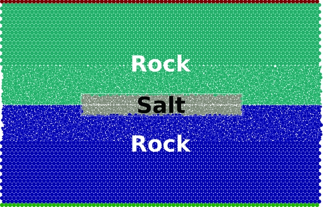
The model consists of a rough planar (1D) fault embedded in a 2D elastic medium, with an added block of material representing a salt lens in the central section of the fault (Fig. 8). This geometry is chosen as it mechanically represents the part of the fault in which salt fills dilational jogs and similar dilatant structures, interrupted by connected host rock from hanging- and footwall. We suggest that the combination of salt lenses and connected but faulted host rock dominates the mechanical properties of the fault zone. The length of the salt block is 50% of the total length of the model, with an aspect ratio of 6:1. The box shape of the block was chosen to simplify the model set-up. At the top and bottom edges of the model a defined normal stress and shear rate are applied; both are held constant after an initial ‘ramp-up’ phase. On the lateral sides of the model, periodic boundary conditions have been applied to enable arbitrary shear displacements without a change in the large-scale geometry of the model.
Geometry of the simple DEM fault model. The two blocks of brittle–elastic ‘rock’ material in blue and cyan, the ductile ‘salt’ material in grey. Green/red edge particles are bonded to the driving plates.
The model internally uses ‘Model units’ requiring a conversion to ‘Real world units’ to compare the results to real data. However, given that there is a free parameter in the conversation between ‘Model’ and ‘Real world’ units (Place et al., Reference Place, Lombard, Mora and Abe2002) the models are scale-free and can be seen as representative of both the laboratory-scale analogue models and the field-scale examples. We therefore do not attach a length scale to the models. A total of eight simulations were used for the parameter study, using four different values for the viscosity parameter A (0.1, 0.25, 1.0 and 2.5) and a slow and a fast loading rate for each of them. The loading rates chosen were 10−5 model velocity units and 10−6 model velocity units. Given that the P-wave velocity in the model is v P=1.0 model unit, this would be equivalent to a few cms−1 to a few mms−1 depending on rock type. This is of course a lot higher than the realistically expected long-term deformation rates for natural faults, but it strikes a balance between realistic values and computational feasibility. The chosen velocities are sufficiently slow that the loading of the fault does not interfere with dynamic processes during slip events which occur at velocities between a few ms−1 (fault slip) and kms−1 (slip propagation). On the other hand, those velocities enable the simulation of statistically valid event catalogues with several thousand slip events in a practical time on a standard multicore workstation (hours to tens of hours).
Additionally, during the inter-event time the ratio between the kinetic energy due to particle movement and the stored elastic energy in the models is low enough to consider the models to be still in a quasi-static regime. While the exploration of slower deformation rates would have been desirable, reducing the deformation rate by another order of magnitude to 10−7 model units would have resulted in an increase of the computing time into the range of weeks and was therefore not done.
Observations
For all models the size distributions of the simulated seismic events were calculated from the time evolution of the elastic energy stored in the material as described above. The results (Fig. 9) strongly suggest a loading rate dependence of the frequency–size distributions of the events. The simulations with the slower loading rate (10−6) produce event size distributions showing a trend towards more frequent large events compared with the simulations using a faster loading rate (i.e. 10−5). However, the size of the largest events remains unchanged. These observations apply independently of the salt viscosity parameter used in the models. It is important to note that the models with different loading rates were run for the same amount of total shear displacement, not the same amount of time.
Frequency–magnitude distribution of the seismic events detected during a simulation using a fault with a salt block for four different values of the salt viscosity defined by the dashpot damping parameter: (A) a=0.1, (B) a=0.25, (C) a=1.0, (D) a=2.5. Open symbols always show the faster loading models; filled symbols show the slower models.
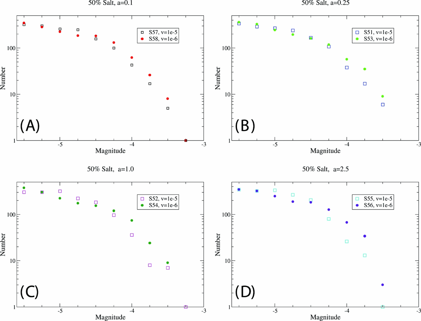
This initially counterintuitive result, i.e. more large events during a given amount of fault displacement at slower loading rates, can possibly be explained by the time evolution of the elastic energy stored in the rock- and salt parts of the model during different parts of the stick-slip cycle. For all models investigated, the data suggest that during inter-seismic times, i.e. the period between the events, relatively little elastic energy is stored in the salt block because salt has enough time between events to completely relax. Therefore, at the loading rates and salt viscosity used in the models, the salt does not contribute to the co-seismic energy release. During and immediately after a large event, however, stress, and therefore elastic energy, is transferred to the salt by the co-seismic movement of the adjacent ‘rock’, i.e. whenever there is a large slip event the amount of elastic energy in the salt is increased. Therefore, after a large event, slip events are suppressed, and the energy available for subsequent events is reduced. In contrast to the slow loading models the relaxation time of the salt in the fast loading models covers a longer part of the typical inter-event time, therefore a stronger reduction in the size of the subsequent events occurs in the fast runs.
This mechanism will not be applicable to models where the salt retains sufficient stored elastic energy between events to actually make a positive contribution to the energy release of the events. This would be expected in case of very high salt viscosity or high loading rates. However, this part of the parameter space has been inaccessible to the present study due to limitations of the DEM implementation used. Specifically, very high values of the viscosity parameter A would require a corresponding reduction in the size of the time step in the models to maintain numerical stability and therefore increase the required computing time beyond what was considered feasible for this work.
Complex fault zone model
To investigate the feasibility of integrating more complex geometries, resembling possible realistic fault zone architectures, into the modelling approach a second set of numerical models was implemented. This geometry is based on the observations from analogue models that, deeper in the fault, salt is distributed in a patchy pattern, which in 2D can be represented as lenses of salt.
Model set-up
For this purpose a set of models was constructed which contain a number of fault rock lenses between the two blocks of wall rock (Fig. 10). The wall rock has the same properties as in the previous models, i.e. it consists of particles fully connected by bonded interactions. Of the lenses, one is filled with salt material (purple particles in Fig. 10), whereas the other lenses consist of rock material. On the interfaces between different fault rock lenses and between a fault rock lens and the wall rock the particles interact by breakable bonded interactions similar to those within the rock material, but with a much lower breaking strength. Colours in Figure 10 represent bodies of coherent particles that are separated by bonded interactions of lower breaking strength. In the models used in the present work the cohesion of the inter-lens bonds was set to 0.0003 model stress units which, assuming elastic properties of typical crustal rocks as scaling parameters, would be equivalent to cohesion of ~10MPa, thus representing a plausible strength level for a partially healed fault surface.
2D DEM model of a more complex fault zone containing salt. Model with an isolated salt lens on the left, with a continuous salt layer on the right. Grey: wall rock; purple: salt; other colours: bodies of coherent particles (rock lenses) that are separated by bonded interactions of lower breaking strength.
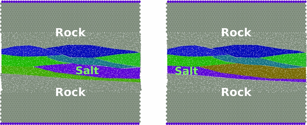
A total of eight simulations has been run for this section, using two different model set-ups and three different values for the salt viscosity (a=0.25, a=1.0 and a=2.5) each. In addition, the models with a viscosity parameter a=1.0 were run using two different shear loading rates, v=10−5 and v=10−6. The two model set-ups differ only in the choice of which of the fault lenses was set up to contain salt instead of fault rock. In the first model (Fig. 10, left), a lens spanning about half the width of the model was chosen whereas in the second model (Fig. 10, right) a lens spreads over the entire width.
Observations
The results show a strong dependence of the mode of deformation in the complex fault models on the way the salt is distributed within the fault zone. If the salt lens covers only about half of the total length of the fault zone (Fig. 10 left) the deformation is localised at a number of the weak interfaces between different fault rock lenses (Fig. 11 left; strong colour contrasts show localised deformation). In contrast, if there is a continuous salt layer spanning the whole length of the fault zone (i.e. Fig. 10 right) the deformation is almost entirely contained within the salt layer and the interface between the salt layer and the fault rock (Fig. 11 right). Due to the different deformation distributions the resulting dynamic behaviour of the two models is also strongly different.
Distribution of x- (horizontal) displacement in a model of a more complex fault zone containing salt. Model with an isolated salt lens on the left, with a continuous salt layer on the right. Blue colours: particles moved towards +x (right); red colours: particles moved towards –x (left).

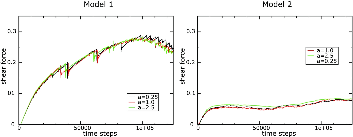
The time evolution of the shear force needed to maintain a constant rate of shear deformation (Fig. 12) shows that the dynamic behaviour of the fault models depends on the geometry of the salt inside the fault zone, the loading rate and the viscosity of the salt. The model with a continuous salt layer exhibits low strength and nearly aseismic creep (Fig. 12 right). In contrast, the model with a salt lens covering only part of the length of the fault zone shows much higher strength and pronounced stick-slip behaviour (Fig. 12 left). In the model with a continuous salt layer the differences are restricted to a small variation in the overall strength of the fault (Fig. 12 right). In the other models a change in timing, size and number of stick-slip events can be observed (Fig. 12 left).
Shear force evolving over time for simulations based on a model with a salt lens (A) or a salt layer (B). Different colours show data from model with different salt viscosities.
Discussion
Salt distribution in dilatant faults
Our analogue experiments show developing fault and fracture networks that are very similar to those observed in experiments without viscous cover layer (Holland et al., Reference Holland, Urai and Martel2006; van Gent et al., Reference van Gent, Holland, Urai and Looseveld2010; Abdelmalak et al. Reference Abdelmalak, Mourges, Galland and Bureau2012; Galland et al. Reference Galland, Holohan, van Wyk de Vries, Burchardt and Németh2015). The excavated hardened resin that preserves the fracture network in 3D shows a distribution of dilatant patches similar to observations made by Holland et al. (Reference Holland, van Gent, Bazalgette, Yassir, Strating and Urai2011) in 3D X-ray CT-scans of dilatant fault experiments. This shows that in the given relationship of cohesion, viscosity and displacement velocity the salt does not strongly affect the fault zone structure but simply flows downward under the influence of gravity. In nature the driving force for this process is the density difference between the rock salt and the saline pore fluid.
In general, the salt distribution within the fault zone is divided into two structural domains, which are likely to have different mechanical properties:
-
1. The uppermost part of the fault zone, where faults are strongly dilatant and salt separates hanging wall and footwall completely.
-
2. The deeper parts of the fault zone, where dilatant faults change to hybrid or shear faults. Here the salt fills dilatant patches of the fault, but hanging wall and footwall are still frictionally mechanically connected in shear-failure patches.
We hypothesise that the faults’ failure mode strongly influences the frequency and magnitude of seismic events in the presence of salt, as faults failing in hybrid tensile/shear mode show significantly stronger coupling between footwall and hanging wall (Kettermann & Urai, Reference Kettermann and Urai2015) than faults failing in pure tensile mode. Our first estimates of stress and strength relationship of the Zechstein carbonates and anhydrites imply a failure in tensile or hybrid tensile/shear mode. However, to correctly predict the precise failure mode of the faults in Groningen in detail and 3D, a much more sophisticated approach towards the estimation of mechanical properties and timing of faulting and salt movement is necessary. As evidence for dilatancy in faults is hardly ever found in seismic data or drill cores due to the low resolution and unidimensional sampling, respectively, a geomechanical modelling approach appears most promising to determine fault behaviour and salt distribution.
Salt flow in fractures
An important outcome of the analogue models is that salt can flow into the dilatant portions of the fault zone during faulting in geological settings similar to the Groningen field. This is strongly controlled by the salt viscosity, fracture aperture and pressure gradient between the salt and the fluid pressure in the dilatant faults. Before the onset of faulting the stress in the viscous salt can be expected to be near-isotropic (differential stress below 2MPa). The opening of a dilatant fault changes the vertical stress in the salt directly above the dilatant fault, producing high differential stresses of more than 20MPa in 2.5km depth. Considering steady-state dislocation creep (Wawersik & Zeuch, Reference Wawersik and Zeuch1986), effective salt viscosities down to 1014Pas can be expected at the depth and temperatures of the present-day base of the Zechstein above dilatant faults.
We apply a simple 2D finite element model using ABAQUS software to simulate the initial flow velocity of salt entering an open fracture (model geometry in Fig. 12A). The results show initially high vertical flow rates up to 13cma−1 for a 1m wide fracture, decreasing to 1cma−1 for a 0.1m wide crack. At later stages, when salt moves between fracture walls, FE models show a Poiseuille-type flow (Fig. 12B–D). Vertical salt velocity decreases with decreasing fracture aperture following a power law function. With 87cm/10,000 years for a 1m wide crack and 0.43cm/10,000 years for a 0.1m wide crack the flow is much slower.
Additionally, due to limited permeability of the sub-salt rocks, the fluid pressures in the faults could be much lower than hydrostatic, directly after the opening. This would produce even higher differential stresses and therefore faster salt flow.
A full understanding of the processes by which salt can move downwards into a fracture requires much more work.
Effect of salt in a fault on seismic event statistics
The results obtained from the DEM-based simulations of the seismicity of faults containing salt lenses show that the chosen approach is suitable for modelling the complex interplay between the ductile behaviour of the salt and the stick-slip dynamics of faults in brittle rocks. In particular, the distribution of seismic event sizes calculated from the simulation data strongly suggests a dependence of the event size distributions on the loading rate if salt is present in the fault zone. The second set of simulations, with variable geometry, also suggests that the mechanical behaviour of the fault is strongly dependent on the geometry of the salt distribution inside the fault zone, i.e. whether the salt forms a continuous layer or an isolated lens. However, since the mechanical properties of the ductile material in the DEM models do not yet exactly match the properties of salt, those results should be taken as a qualitative indication of the influence of salt on the dynamic behaviour of faults.
In order to enable a more quantitative investigation of the influence of salt on the dynamic behaviour, in particular with regard to the details of the rheology of the salt, an extension of the DEM approach used would be necessary. Possible avenues in that direction would be the implementation of a Maxwell material instead of a Voigt–Kelvin material at the particle scale in the DEM formalism or a coupling between the DEM approach and a Smooth Particle Hydrodynamic (SPH) model. The latter approach has been shown the to be feasible (Komoróczi et al., Reference Komoróczi, Abe and Urai2013; Robinson et al., Reference Robinson, Ramaioli and Luding2014) and to be applicable to the modelling of coupled brittle–ductile problems (Komoróczi et al., Reference Komoróczi, Abe and Urai2013). Furthermore, an extension of the model to include the effect of a full 3D geometry would be desirable.
Conclusions
We used a combination of analogue and numerical modelling to investigate possible effects of salt in dilatant fault zones on the frequency and magnitude of seismic events in a setting comparable to the Groningen gas field. Under the assumption that the carbonates and anhydrites beneath the Z3 and Z4 salts of the Groningen area form faults in hybrid or dilatant failure, the presented analogue models clearly show that salt analogue flows downwards into the opening fractures and faults in underlying brittle rocks. The system gains complexity by lateral flow of the salt, which brings salt into extensional jogs even beneath non-dilating parts of the fault zone. The extent to which salt will flow into a fault zone is strongly controlled by the failure mode of the underlying rocks, the structural domain of the fault (i.e. precursor or graben domain) and the overall fault geometry.
Using this information as input for numerical models, we have shown that the DEM approach is suitable to obtain qualitative insight into the seismicity of faults containing salt or other ductile materials. Our first tests have shown that the presence of salt in a fault zone has the potential to make the dynamic behaviour of the fault dependent on the shear loading rate, including the modification of the frequency–magnitude distribution of the generated seismic events. While some trends have become visible, large parts of the parameter space of fault geometry, salt rheology and loading rate remain unexplored and the complex interplay between stick-slip dynamics of a fault and the viscoelastic behaviour of the salt contained in it is not really understood so far. This opens up new exciting opportunities for future research.
Acknowledgements
Hans de Bresser and an anonymous reviewer are thanked for their thorough reviews that helped to improve the article. Clemens Visser is thanked for providing information on faulting in the Groningen field. This project was funded by Staatstoezicht op de Mijnen, Ministerie van Economische Zaken, the Netherlands.


 Open access