





Introduction
As glaciers melt, global sea level is projected to rise (Golledge and others, Reference Golledge2019; Fox-Kemper and others, Reference Fox-Kemper and Masson-Delmotte2021). At the same time, the input of freshwater into the ocean is expected to increase (Bamber and others, Reference Bamber2018; Pellichero and others, Reference Pellichero, Sallée, Chapman and Downes2018), altering ocean salinity and influencing meridional overturning circulation (Proshutinsky and others, Reference Proshutinsky, Dukhovskoy, Timmermans, Krishfield and Bamber2015; Golledge and others, Reference Golledge2019; Li and others, Reference Li, England, Hogg, Rintoul and Morrison2023). The uncertainty in the rate of frontal ablation of tidewater glaciers in polar regions, which includes both iceberg calving and submarine melt, is one of the largest contributors to uncertainty in projections of the timing and magnitude of future sea level rise (Fox-Kemper and others, Reference Fox-Kemper and Masson-Delmotte2021). However, submarine melt rates remain relatively unconstrained, in part due to the challenges and dangers associated with working at the face of large icebergs or an actively calving glacier.
Field measurements at Xeitl Sít’ (also known as LeConte Glacier) in Alaska in 2018 indicate that the standard melt theory, which combines the three-equation model (McPhee and others, Reference McPhee, Maykut and Morison1987; Holland and Jenkins, Reference Holland and Jenkins1999) with plume theory (Jenkins, Reference Jenkins2011; Jackson and others, Reference Jackson2017), underestimates observed melt rates when averaged across the ice face by more than an order of magnitude (Sutherland and others, Reference Sutherland2019; Jackson and others, Reference Jackson2022). While plume theory can predict locally high melt rates within regions of focused subglacial discharge, it substantially underestimates background melt in areas away from plumes. The resulting spatially averaged modeled melt rates are therefore much lower than those inferred from observations. This discrepancy between observations and model predictions suggests that key physical processes are missing from current models. Possible explanations include (i) simplified representations of near-ice circulation and turbulence (Jackson and others, Reference Jackson2020; Nash and others, Reference Nash2024; Weiss and others, Reference Weiss2025), (ii) failure to account for internal waves (Cusack and others, Reference Cusack2023), (iii) simplifications of the physics associated with ice material properties (Wengrove and others, Reference Wengrove, Pettit, Nash, Jackson and Skyllingstad2023) and (iv) the assumption of smooth ice faces instead of realistic morphologies (Schild and others, Reference Schild, Sutherland, Elosegui and Duncan2021; Abib and others, Reference Abib2023; Schmidt and others, Reference Schmidt2023). Here, we explore the latter source of uncertainty by characterizing submarine iceberg morphology, which is distinct from glacier termini but still provides important insight for improving the parametrization of ice-face geometry in melt models.
Many studies have shown that surface roughness significantly alters velocity profiles within turbulent boundary layers by disrupting the flow and generating localized motions known as turbulent eddies. These eddies enhance mixing near the boundary, thereby increasing surface drag and the transfer of heat, salt and momentum (Kadivar and others, Reference Kadivar, Tormey and McGranaghan2021). At an air–ice interface, studies have shown that even small increases in the mean roughness height can substantially increase aerodynamic roughness length scales and sensible heat flux (Munro, Reference Munro1989; Chambers and others, Reference Chambers, Smith, Quincey, Carrivick, Ross and James2020). Although similar processes are thought to occur at ice–ocean interfaces, direct observations of submarine ice roughness remain sparse. Numerical simulations and laboratory experiments have demonstrated that turbulent structures near the ice face control local melt rates (Kerr and McConnochie, Reference Kerr and McConnochie2015; Gayen and others, Reference Gayen, Griffiths and Kerr2016), but observational constraints on roughness parameters in these environments are limited.
Ice–ocean boundary morphology spans a range of spatial scales, but significant gaps persist in our understanding of medium- to small-scale features  $\mathcal{O}$(0.5–5 m) relevant to ambient submarine melt. At large scales $\mathcal{O}( \gt 500\,\text{m})$, roughness may be associated with undulating basal topography beneath ice shelves, where studies such as Watkins and others (Reference Watkins, Bassis and Thouless2021) have shown that topographic variability, quantified using both root-mean-square (RMS) height and spectral metrics, can influence ice dynamics and basal melt rates. Watkins and others (Reference Watkins, Bassis and Thouless2021) found that roughness follows a power-law scaling and is strongly correlated with melt, suggesting that morphological variability contributes not only to enhanced basal melt but also to increased fracturing, rifting and decreased ice shelf stability. More recent work indicates that strain rates can also influence roughness at localized scales by promoting fracturing, acting together with melt to shape ice morphology (Watkins and others, Reference Watkins, Bassis, Thouless and Luckman2024). While such studies focus on ice shelves and kilometer-scale basal features, they provide an important precedent for using statistical and spectral approaches to relate ice morphology to melt.
At smaller spatial scales  $\mathcal{O}$(1–100 m), roughness becomes increasingly relevant to boundary layer dynamics. Observations beneath Thwaites Glacier revealed ice terraces with relief up to 6 m and channel-like features as wide as 50 m (Schmidt and others, Reference Schmidt2023). Finer-scale features such as scallops and ridges, with amplitudes of 0.1–0.5 m and spacings of 2–5 m, have also been documented on submarine ice faces (Schmidt and others, Reference Schmidt2023). Ice scallops, in particular, have been investigated through modeling and laboratory studies (Bushuk and others, Reference Bushuk, Holland, Stanton, Stern and Gray2019; Wilson and others, Reference Wilson, Vreugdenhil, Gayen and Hester2023; Yang and others, Reference Yang, Howland, Liu, Verzicco and Lohse2023; Sweetman and others, Reference Sweetman, Shakespeare, Stewart and McConnochie2024), and are thought to arise from feedbacks between turbulent flow and melt. Despite these advances, roughness features in the 0.5–5 m range remain underexplored in observational datasets, particularly along near-vertical glacier and iceberg faces where direct access is limited.
In this context, roughness refers to morphological variability superimposed on the bulk geometry of the ice face. Across disciplines, roughness has been defined in various ways to capture structural complexity. In reef ecology, for example, McCormick (Reference McCormick1994) characterized roughness in terms of rugosity, incorporating vertical relief and angular variability relative to a horizontal reference line. In landscape ecology, Du Preez (Reference Du Preez2015) defined rugosity as the ratio of true surface area to the area projected onto a plane of best fit, using this metric to quantify three-dimensional landscape complexity. Friedman and others (Reference Friedman, Pizarro, Williams and Johnson-Roberson2012) similarly defined rugosity as a surface area-based metric, and used it to evaluate how topographic complexity varies across spatial scales in 3D bathymetric surfaces. Building on these definitions, we adopt a rugosity metric and apply a spectral approach to quantify surface variability, chosen because it provides a scale-resolved look at roughness and identifies how different length scales contribute to the total morphology. We then apply it to 13 sonar derived iceberg surfaces and one drone derived surface from a recently capsized iceberg. By decomposing each surface, we distinguish between iceberg-scale morphology  $\mathcal{O}$(10 m) from medium- to small-scale roughness $\mathcal{O}$(0.5–5 m), providing a scale-resolved assessment of how ice morphology enhances the effective ice–ocean interface. These observations support a pathway toward incorporating realistic roughness statistics into ice–ocean melt models.
Methodology
Field campaigns
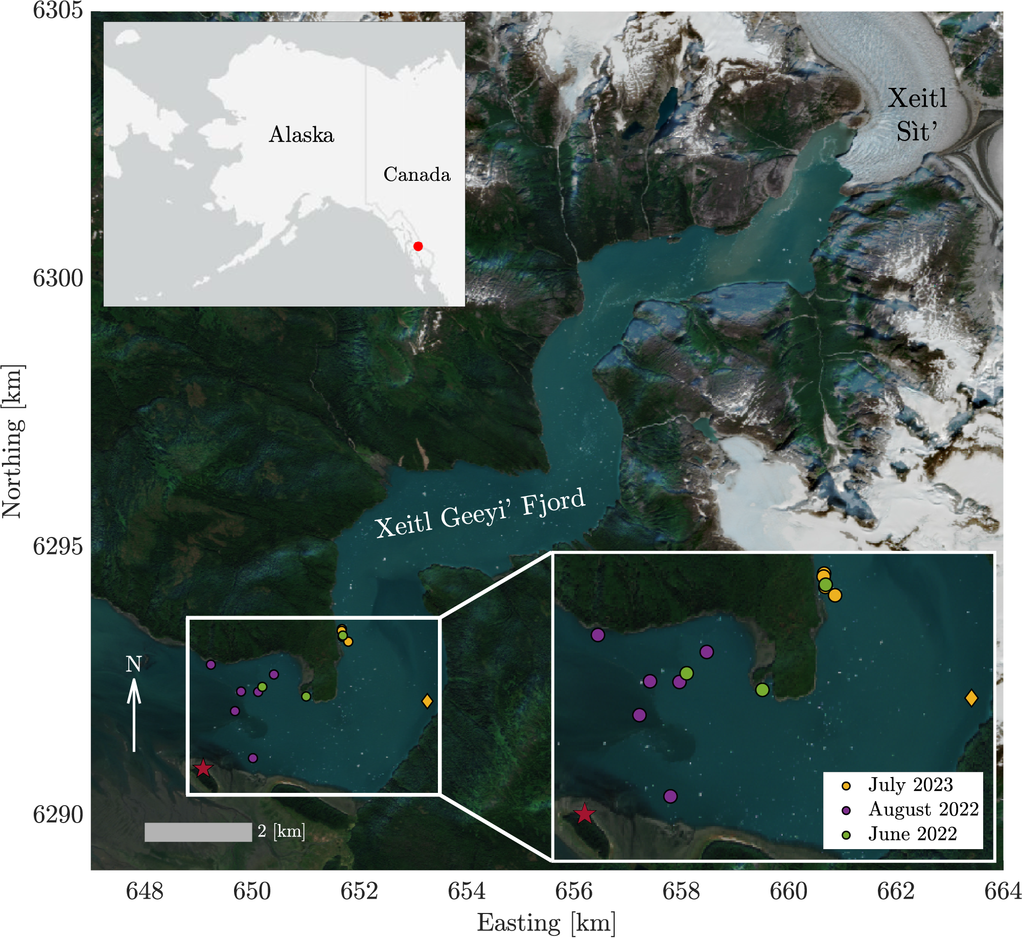
Iceberg morphology measurements were collected from 14 icebergs in Xeitl Geeyi’ during three field campaigns between spring 2022 and summer 2023 (Fig. 1). Thirteen of the icebergs were grounded, and one was floating. Grounded iceberg surfaces were surveyed using Norbit iWBMS, Winghead i77h or Winghead i80s multibeam sonars (Norbit Subsea AS, 2023) mounted on small boats. The iWBMS sonar head was mounted on the side of the boat and oriented toward the ice face (Abib and others, Reference Abib2023), while the Winghead sonars were downward-facing with beams electronically steered toward the ice face. Surveys were conducted from distances ranging from approximately 3 to 10 m from the ice face. At these distances and for a maximum depth of 40 m, the beam footprint of the multibeam sonar system remained relatively small in both the down-ice and along-ice directions. In the along-ice (horizontal) direction, footprint size was determined by vessel speed and ping rate; for speeds of 3 knots and 5 knots, the horizontal resolution ranged from approximately 0.06–0.085 m. In the down-ice (vertical) direction, beam spreading increased with depth, with footprint sizes reaching approximately 0.1 m near the surface and up to 0.5 m at 40 m depth. The floating iceberg was surveyed using a DJI Air 2S drone shortly after the iceberg flipped, exposing a previously submerged surface. All surveyed icebergs were located 15–20 km downstream from their origin at Xeitl Sít’ and were named after characters from Alice in Wonderland (Carroll, Reference Carroll1865), with these names occasionally used throughout the manuscript. Although icebergs are located downstream from the glacier terminus, the near-vertical faces of icebergs provide accessible analogs for studying ice–ocean boundary roughness at field scale. These observations therefore complement, but do not replace, direct measurements at the glacier terminus.
Map of Xeitl Geeyi’ in southeastern Alaska, with its location indicated by a red dot on the inset map of Alaska. Grounded icebergs surveyed with the multibeam sonar are shown as circles, while the iceberg surveyed using a drone is represented by a diamond. All surveyed icebergs originated from Xeitl Sít’ and are colored according to the field campaign during which they were studied. The location of the base station is marked with a red star.

Temperature, conductivity and pressure in the water column were measured using an RBR Concerto profiler (RBR Ltd., 2023) to derive sound speed for correcting multibeam acoustic paths. Profiles were collected within approximately 15 m of each iceberg, with 1–3 casts acquired per iceberg to account for vertical structure in sound speed. Conductivity measurements were corrected for sensor time lag, and salinity and sound velocity profiles were derived using MATLAB functions from the RSKtools MATLAB toolbox (v3.6.1).
Multibeam sonar processing
Multibeam sonar data of the grounded icebergs were processed in Qimera. First, the sound velocity correction was applied to the multibeam data using the SVP cast taken closest to it in time. Geodetic referencing for the multibeam data was adjusted using Post-Processing Kinematic (PPK) corrections from the local base station measurements with POS-PAC software, reducing uncertainty in the ( $x,y,z$) location of the soundings as a function of time. PosPac processing resulted in horizontal position accuracies ranging from 2–5 cm and vertical position accuracies ranging from 5–10 cm. The base station measurements were collected from a Trimble R-12 or Hemisphere S321 base station that was temporarily set up over the same ground point marked by a re-bar rod driven into the ground on Camp Island (red star in Fig. 1). Finally, the multibeam data were corrected for position and then manually cleaned to remove outliers, defined as isolated or spurious returns clearly inconsistent with the surrounding ice surface. Iceberg motion required surfaces to be generated from single-pass surveys, while variability in sound speed close to the ice face ( $ \lt $5–10 m, not always captured by CTD casts) introduced additional potential error in acoustic path corrections. Undercut regions of the ice face also frequently became shadow zones due to sonar geometry, resulting in gaps or underrepresentation in the shallowest undercut surfaces. Apparent artifacts, such as false ridges or ‘Erik’s horns’ (Jakobsson and others, Reference Jakobsson2016), were also manually removed.
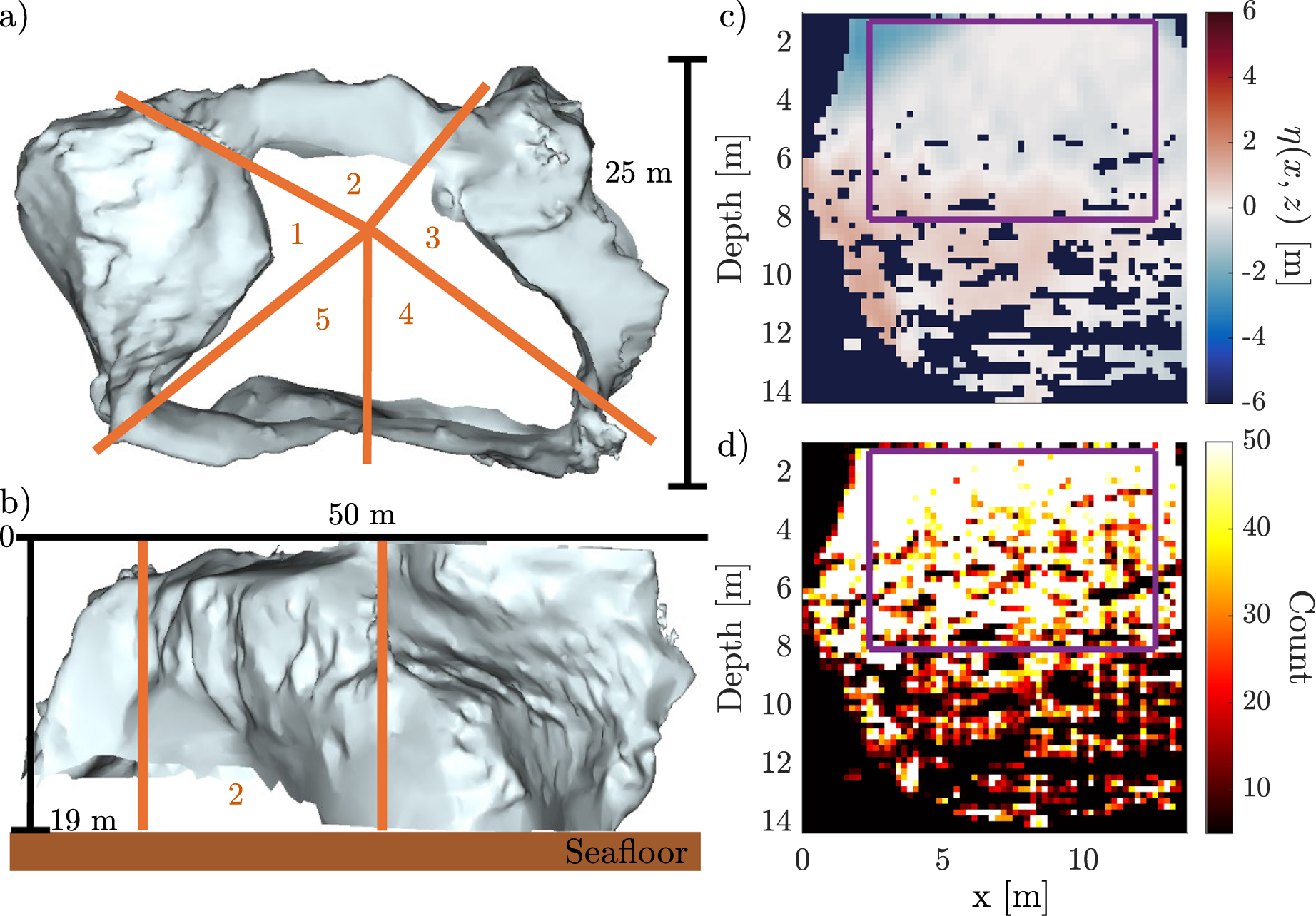
From the 13 grounded icebergs, 54 sides were extracted, from which 54 surfaces were derived from multibeam sonar data. Each side was defined as a continuous surface with relatively consistent curvature, such that the normal plane varied by no more than  $\sim30^\circ$ along the surface (Fig. 2a). Regions with large data gaps or shadowing were further subdivided (e.g., sides 4 and 5 in Fig. 2a). For each side, a best-fit plane was computed from the 3D point cloud. This plane was oriented parallel to the $z$ direction to represent the local mean orientation of the ice face. The plane was then used to detrend the data in the along-ice ( $x$) direction, setting the mean along-ice gradient to approximately zero while preserving the vertical-ice ( $z$) slope, where $z$ is positive down. The detrended point cloud was gridded onto the $xz$-plane at 20–40 cm resolution, depending on point density (Fig. 2d). Grid cells with fewer than five points were assigned NaN values. From each surface, the region with the highest point density (purple box in Fig. 2c-d) was extracted, and missing values within this region were linearly interpolated to create a continuous gridded surface. In this final surface, $\eta(x,z)$ represents the relief, defined as the perpendicular distance from the best-fit plane, at each $x$ and $z$ location (Fig. 3a), with mean relief approximately zero due to detrending.
a) Top-down and b) side view of a 3D rendering of the underwater portion of the iceberg Dormouseberg. The dimensions of this iceberg were approximately 50 m in length, 25 m in width and it was grounded on the seafloor at a depth of 19 m, with the ocean surface represented by the 0 line. The iceberg was divided into five sides (orange lines in a,b), each subsequently gridded as a separate surface ( $\eta(x,z)$). c) Side 2 of this iceberg gridded at a 20 cm resolution. $x$-axis shows the distance along the ice surface in meter, $z$-axis represents the depth in meter and color bar indicates the relief of the surface ( $\eta(x,z)$) in m. d) 2D histogram of point density on side 2. The color bar shows the number of points per grid cell. The selected surface ( $\eta(x,z)$) for subsequent analysis is the region bounded by the purple box in c) and d), where the data density is highest. Dark blue-grey patches in c correspond to grid cells with fewer than five points and match the black patches in d.

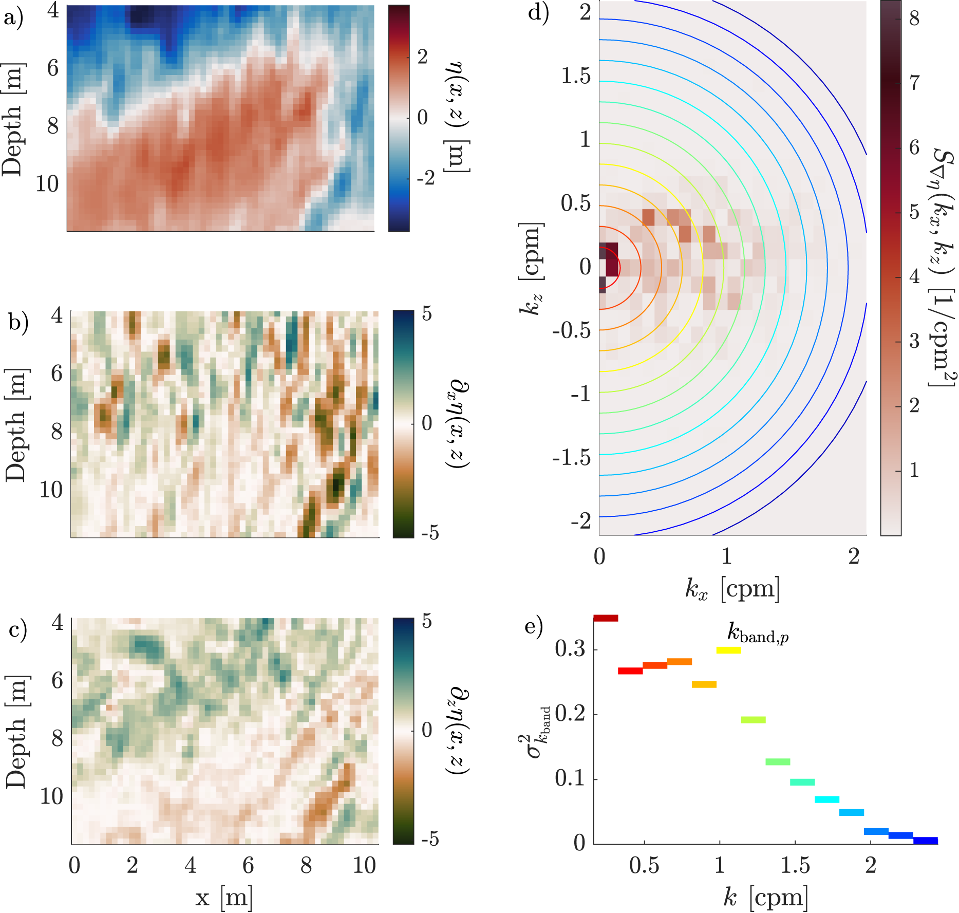
Slope spectra technique: a) Example of a 20 cm gridded iceberg surface ( $\eta(x,z)$), shown in the $xz$-plane. b) Gradient of the surface in the along-ice ( $x$) direction ( $\partial_x\eta(x,z)$). c) Gradient in the vertical ( $z$) direction ( $\partial_z\eta(x,z)$). d) Combined 2D PSD of $\partial_x\eta(x,z)$ and $\partial_z \eta(x,z)$, where each semi-annular region between contours defines a wavenumber band ( $k_{\text{band}}$). e) Slope variance ( $\sigma^2_{k_\text{band}}$), plotted as a function of $k$. Colors in e correspond to the annular bands in d. Where multiple local maxima occur (e.g., near $k\approx0.75$ cpm and $k\approx1$ cpm in panel e), the characteristic length scale ( $\lambda_p$) is defined by the maximum with the largest slope variance ( $k_{\text{band},p}$).

Structure-from-motion (SfM) processing
One continuous gridded surface was produced from a single side of the floating iceberg (named Queenofheartsberg), which was extracted and processed using SfM techniques in Agisoft Metashape. The previously above-water portion of the iceberg was set to  $z=0$, and a best-fit plane was removed in both the along-ice ( $x$) and vertical ( $z$) directions. The resulting 3D point cloud was gridded in the $xz$-plane at 5 cm resolution.
Ice morphology metrics
In total, 55 surfaces ( $\eta(x,z)$) were analyzed from multibeam sonar and drone-based surveys. To characterize the roughness of each surface, the distribution of slope variance across spatial scales was analyzed. Surfaces lacking a discernible local maximum in slope variance were classified as exhibiting broadband variance, meaning that variance is distributed across a broad range of spatial scales, and are referred to here as ‘broadband roughness’. Surfaces with identifiable peaks were classified as having a component of narrowbanded variance within the signal and are therefore referred to as ‘narrowband roughness’ for the remainder of this manuscript. Here, ‘identifiable’ denotes a discernible peak in the slope-variance distribution, used qualitatively to distinguish surfaces showing concentrated variance at a given scale from those without concentrated variance. For these surfaces, $\eta(x,z)$ was decomposed into iceberg-scale morphology ( $\bar{\eta}(x,z)$) and medium- to small-scale roughness ( $\eta\prime(x,z)$) to isolate different morphological length scales:
 \begin{equation}
\eta(x,z)=\bar{\eta}(x,z)+\eta\prime(x,z).
\end{equation}
\begin{equation}
\eta(x,z)=\bar{\eta}(x,z)+\eta\prime(x,z).
\end{equation}Surfaces exhibiting broadband roughness were excluded from this decomposition because the absence of an identifiable peak precludes separation into iceberg-scale morphology and medium- to small-scale roughness. This decomposition enabled the application of statistical and spectral analyses to quantify metrics of surface variability, including wavelength, RMS height, relief distribution and anisotropy.
Slope spectral analysis
Slope variance across spatial scales was quantified using the power spectral density (PSD),  $S_{\nabla\eta}(k_x,k_z)$, computed from 2D Fourier transforms of surface gradients of $\eta(x,z)$ ( $\nabla\eta(x,z)$) in the $x$- and $z$-directions ( $\partial_x\eta(x,z)$ and $\partial_z\eta(x,z)$). The total slope PSD is defined as:
 \begin{equation}
S_{\nabla\eta}(k_x,k_z) = S_{\partial_x\eta}(k_x,k_z)+S_{\partial_z\eta}(k_x,k_z)
\end{equation}
\begin{equation}
S_{\nabla\eta}(k_x,k_z) = S_{\partial_x\eta}(k_x,k_z)+S_{\partial_z\eta}(k_x,k_z)
\end{equation} where  $k_x$ and $k_z$ are the wavenumber components in the $x$- and $z$-directions. To analyze slope variance as a function of spatial scale, wavenumber bands were defined over discrete intervals $k_{\text{band}}\in[k_{\text{min},\text{band}},k_{\text{max},\text{band}}]$, where each band corresponds to a semi-annular region of constant wavenumber (contours in Fig. 3d). The width of each band was determined by the spectral resolution in $k_x$ and $k_z$, which varied across surfaces due to differences in grid size and overall surface dimensions of $\eta(x,z)$. The slope variance within each band ( $\sigma_{k_\text{band}}^2$) was calculated by integrating the PSD over the region $R$ described by $k_{\text{band}}$ (i.e., $k_\text{min,band}\leq\sqrt{k_x^2+k_z^2}\leq k_\text{max,band}$):
 \begin{equation}
\sigma_{k_\text{band}}^2=2\int_{R} S_{\nabla\eta}(k_x,k_z) dk_xdk_z .
\end{equation}
\begin{equation}
\sigma_{k_\text{band}}^2=2\int_{R} S_{\nabla\eta}(k_x,k_z) dk_xdk_z .
\end{equation} A characteristic length scale ( $\lambda_p$) was determined by identifying the wavenumber band corresponding to an identifiable local peak in the slope variance distribution ( $\sigma_{k_{\text{band},p}}^2$) across wavenumber bands (Fig. 3e). In cases where multiple local maxima were present, the characteristic length scale was taken as the local maximum with the highest slope variance. This approach excludes cases where the largest variance occurs at the lowest wavenumber band, which reflects iceberg-scale surface trends rather than medium- to small-scale features. The wavenumber associated with this peak ( $k_{\text{band},p}$) was used to estimate the dominant spatial scale as:
 \begin{equation}
\lambda_p=\frac{1}{k_{\text{band},p}}.
\end{equation}
\begin{equation}
\lambda_p=\frac{1}{k_{\text{band},p}}.
\end{equation} To ensure spectral peaks were meaningful based on the measurement technique, we imposed bounds based on the grid resolution and size of each surface. The lower limit was set by the multibeam sonar grid resolution (20–40 cm), we require at least four grid cells per wavelength to trust the wavelength measurement, corresponding to a minimum resolvable  $\lambda_p$ of 0.8-1.6 m. The upper limit was set by the continuous ice surface size (mean $\sim10$ m across both directions), we require at least three wavelengths within the continuous ice surface to trust the wavelength measurement, yielding an upper bound on $\lambda_p$ of 3–3.7 m. Peaks outside of these limits were excluded from analysis.
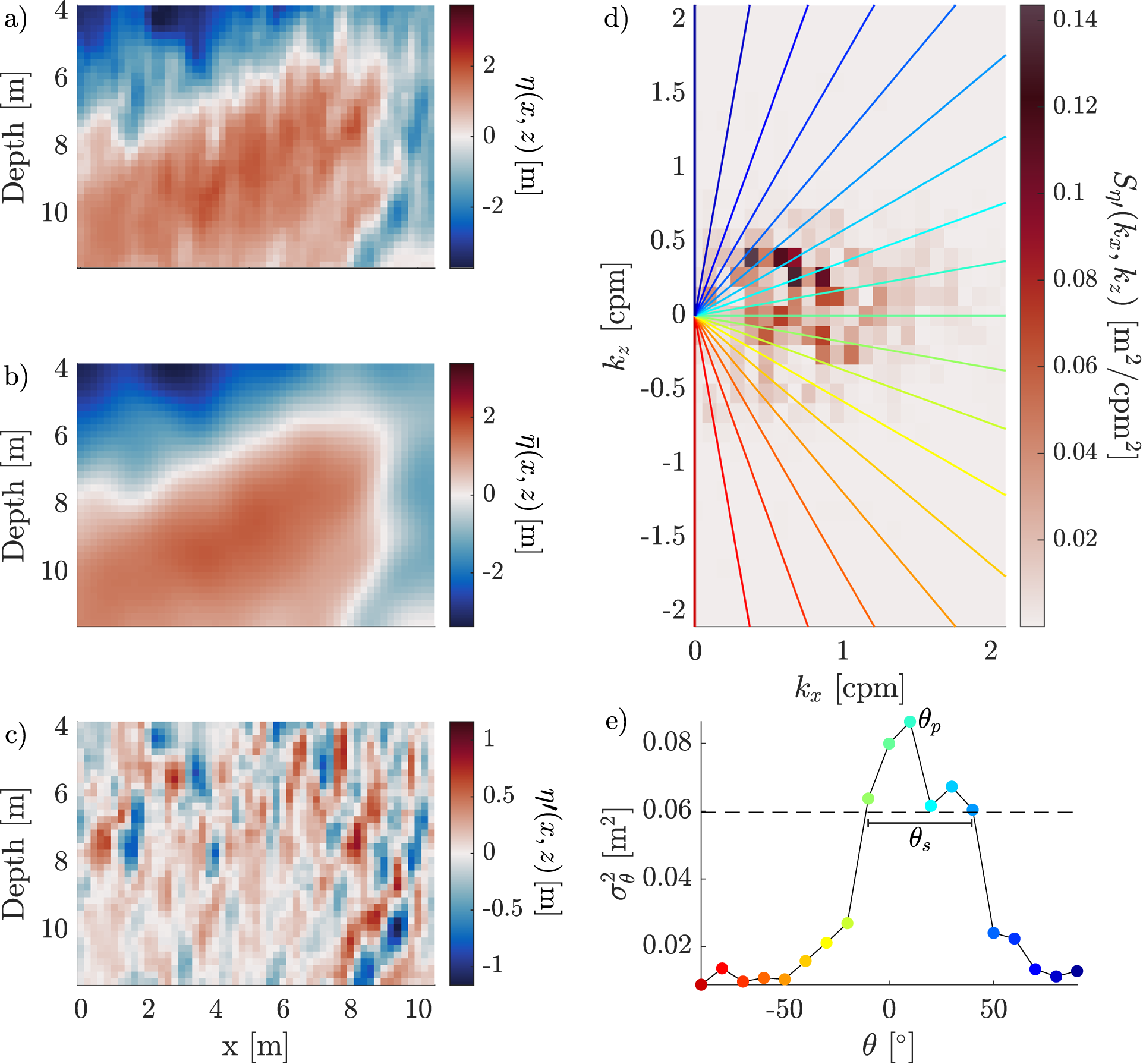
Once the characteristic length scale of a surface was determined ( $\lambda_p$), the surface $\eta(x,z)$ was decomposed into its larger-scale iceberg morphology ${\eta}(x,z)$ and medium- to small-scale roughness $\eta\prime(x,z)$ (Fig. 4a–c). The iceberg-scale component $\bar{\eta}(x,z)$ was obtained by applying a two-dimensional Gaussian low-pass filter to $\eta(x,z)$. This filter computes a weighted average of neighboring values using a Gaussian kernel, where the standard deviation controls the smoothing width. To isolate features larger than the peak wavelength, the standard deviation was chosen such that the filter effectively suppressed components with wavelengths shorter than $\lambda_p$. $\eta\prime(x,z)$ was then calculated by subtracting $\bar{\eta}(x,z)$ from the original surface $\eta(x,z)$ (Eqn 1). Surfaces without a clearly defined $\lambda_p$ were classified as having broadband roughness and therefore excluded from decomposition.
Amplitude spectra technique: a) Gridded iceberg surface ( $\eta(x,z)$) at 20 cm resolution. b) Iceberg-scale morphology ( $\bar{\eta}(x,z)$), obtained using a 2D Gaussian filter on $\eta(x,z)$. c) Medium- to small-scale roughness component ( $\eta\prime(x,z)$), computed by subtracting $\bar{\eta}(x,z)$ from $\eta(x,z)$. d) 2D PSD of $\eta\prime(x,z)$, with radial direction lines spaced at 10 $^\circ$ intervals, corresponding to different orientation angles ( $\theta$). e) Directional variance ( $\sigma^2_{\theta}$) plotted as a function of $\theta$, where the horizontal dashed line indicates the threshold for anisotropy. Colors in e correspond to radial lines in d.

Total rugosity ( $f_{\eta}$) was quantified as the ratio of the three-dimensional surface area to its planar projected area:
 \begin{equation}
f_{\eta} = \frac{\int_A \sqrt{1 + \left(\frac{\partial \eta}{\partial x}\right)^2 + \left(\frac{\partial \eta}{\partial z}\right)^2 } \, dx \, dz}{A_p}
\end{equation}
\begin{equation}
f_{\eta} = \frac{\int_A \sqrt{1 + \left(\frac{\partial \eta}{\partial x}\right)^2 + \left(\frac{\partial \eta}{\partial z}\right)^2 } \, dx \, dz}{A_p}
\end{equation}where  $A$ is the region of the surface $\eta(x,z)$ in the $xz$-plane and $A_p$ is the corresponding projected area. The numerator is the standard surface area integral, which computes the analytical three-dimensional area of a surface from its local slopes. The square-root term arises from the magnitude of the cross product of two adjacent vectors to the surface, capturing how local slopes increase area relative to the projected plane. In this formulation, rugosity is the ratio of the full surface area to its planar projection, such that $f_\eta = 1$ for a perfectly flat surface. For surfaces classified as having broadband roughness (i.e., no identifiable $\lambda_p$), only the total rugosity was computed, as these surfaces could not be decomposed into iceberg-scale and medium- to small-scale components. To assess the role of different spatial scales on narrowband surfaces, rugosity was partitioned into iceberg-scale ( $f_{\bar{\eta}}$) and medium- to small-scale ( $f_{\eta\prime}$) contributions. The iceberg-scale rugosity was computed directly from the smoothed surface $\bar{\eta}(x,z)$, while medium- to small-scale rugosity was computed from the residual surface $\eta\prime(x,z)$. This approach isolates the enhancement of surface area arising from larger-scale morphology versus finer-scale roughness, allowing their individual and combined effects on ice–ocean boundary area to be quantified.
To validate this formulation, we also computed rugosity using a numerical surface-area method, in which each surface was discretized into triangular mesh elements and the three-dimensional surface area was obtained by summing over all triangles. The resulting ratio of true surface area to planar projected area provides an exact geometric definition of rugosity. Comparison between this geometric calculation and Eqn (5) revealed that Eqn (5) systematically underestimates  $f_\eta$ and $f_{\eta'}$, but shows no bias for $f_{\bar{\eta}}$. We therefore applied a mean bias correction to $f_\eta$ and $f_{\eta'}$, derived from their linear fit against the geometric calculation, to ensure comparability with the exact surface area while preserving relative variability across surfaces (see Supplementary Section S1).
Amplitude spectral analysis
The RMS height ( $\text{H}_{\text{RMS}}$) of $\eta\prime(x,z)$ was calculated using its PSD (Fig. 4d), $S_{\eta\prime}(k_x,k_z)$, which was computed from the 2D Fourier transform of the amplitude of $\eta\prime(x,z)$ (Perron and others, Reference Perron, Kirchner and Dietrich2008; Spagnolo and others, Reference Spagnolo2017) as:
 \begin{equation}
\text{H}_{\text{RMS}}=\sqrt{2\int_{-k_{z,\text{max}}}^{k_{z,\text{max}}} \int_{0}^{k_{x,\text{max}}} S_{\eta\prime}(k_x,k_z) dk_x dk_z}.
\end{equation}
\begin{equation}
\text{H}_{\text{RMS}}=\sqrt{2\int_{-k_{z,\text{max}}}^{k_{z,\text{max}}} \int_{0}^{k_{x,\text{max}}} S_{\eta\prime}(k_x,k_z) dk_x dk_z}.
\end{equation} Anisotropy was assessed by computing the variance of  $\eta\prime(x,z)$ as a function of orientation ( $\theta$), sampled from $-90^\circ$ to $90^\circ$ in $10^\circ$ increments. For each orientation, the 2D power spectral density $S_{\eta\prime}(k_x,k_z)$ was rotated about the origin in wavenumber space by the corresponding $\theta$. After rotation, the directional variance ( $\sigma_{\theta}^2$) was computed by integrating the rotated spectrum along the $k_z=0$ axis corresponding to the each orientation:
 \begin{equation}
\sigma_{\theta}^2 = 2 \int_{0}^{k_{x,\text{max}}} S_{\eta\prime}^\theta(k_x, 0) dk_x
\end{equation}
\begin{equation}
\sigma_{\theta}^2 = 2 \int_{0}^{k_{x,\text{max}}} S_{\eta\prime}^\theta(k_x, 0) dk_x
\end{equation}where  $S_{\eta\prime}^\theta$ denotes the spectrum rotated by $\theta$, and $k_{x,\text{max}}$ is the maximum resolvable radial wavenumber in $x$. Surface anisotropy was quantified by analyzing the directional distribution of directional variance across all orientations (Fig. 4e). A strong peak in directional variance around a specific orientation indicates anisotropic roughness, while a more uniform distribution implies isotropy. A threshold for anisotropy is defined as one standard deviation above the mean directional variance across all $\sigma_{\theta}^2$. If a single peak ( $\sigma_{\theta,p}^2$) exceeds the defined threshold, the surface is classified as anisotropic, and the corresponding orientation ( $\theta_p$) is identified as the peak orientation. The directional spread associated with the peak ( $\theta_s$) is defined as the width of the peak at the anisotropy threshold. A peak at $\theta=0^\circ$ indicates vertically aligned (aligned with gravity) roughness features. A narrower directional spread implies stronger anisotropy.
Probability density function analysis
The skewness ( $\mathrm{sk}$) and kurtosis ( $\mathrm{ku}$) of the surface roughness were computed from a probability density function (PDF) of the surface amplitude $\eta\prime(x,z)$ (Kadivar and others, Reference Kadivar, Tormey and McGranaghan2021). Positive $\mathrm{sk}$ indicates an asymmetric surface with more pronounced crests and flatter troughs, while negative $\mathrm{sk}$ reflects surfaces with deeper troughs and flatter crests. A value of zero denotes a symmetric distribution of surface elevations. Kurtosis ( $\mathrm{ku}$) describes the peakedness of the distribution, with values below 3 (platykurtic) indicating broader, flatter distributions and values above 3 (leptokurtic) indicating distributions with more pronounced central peaks and heavier tails. A kurtosis value of 3 is considered mesokurtic and corresponds to a normal distribution.
Results
Observations of submarine iceberg morphology
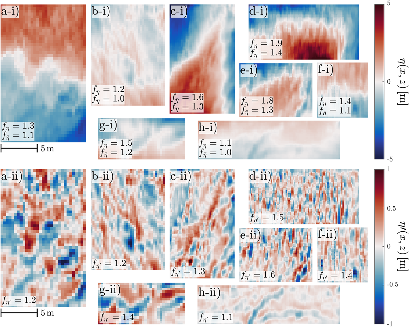
Iceberg shape and roughness were quantified from 55 iceberg surfaces, derived from multibeam sonar measurements of 13 grounded icebergs and from a drone survey of one floating iceberg immediately after it capsized, exposing a previously submerged face. Among the 54 sonar-derived surfaces, dimensions range from 3.2 m to 28.8 m along the ice surface ( $x$) and from 2.8 m to 20 m down the ice surface ( $z$), with a mean extent of $\sim$10 m across both directions. Absolute relief across all surfaces ( $\eta(x,z)$) spans from 0.22 m to 7.78 m. Oscillatory patterns in surface relief are frequently observed in both $x$ (Fig. 5b, c, g) and $z$ (Fig. 5b, h). Iceberg-scale variations include both overcut geometries (top is negative eta, blue and bottom is positive eta, red in Fig. 5b–e, g) and undercut geometries (top is positive eta, red and bottom is negative eta, blue in Fig. 5a, f, h). Several surfaces also exhibit near-vertical faces (No change in color right of Fig. 5d and right of Fig. 5e). Distinct features such as deep channels (Fig. 5g, h) and divots (Fig. 5b) are occasionally evident prior to filtering.
Of the 54 sonar-derived surfaces, 39 exhibit narrowband roughness ( $\eta\prime(x,z)$). Relief within these surfaces ranges from 0.16 m to 2.10 m. The remaining 15 surfaces were classified as broadband and were therefore excluded from the decomposition described by Eqn (1) and $\eta\prime(x,z)$ analysis because no distinct peak was identified in the slope spectra, preventing decomposition into iceberg-scale morphology and medium- to small-scale roughness. Despite large-scale variability in slope and shape, many of the narrowband surfaces display medium- to small-scale channels (Fig. 5a–h). In some cases, channels diverge in different orientations (Fig. 5b, h). Most channels appear nearly vertical (Fig. 5d–f), but several are tilted up to $\sim$45 $^\circ$ from vertical (Fig. 5b, c, g; deep channel in Fig. 5h). Additional visualizations and details for each iceberg and the analyzed surface subsets are provided in Supplementary Section S2.
a-i)–h-i) Observations of eight gridded iceberg surfaces  $\eta(x,z)$ and their corresponding a-ii)–h-ii) medium- to small-scale roughness components $\eta\prime(x,z)$, computed by applying a two-dimensional Gaussian filter to $\eta(x,z)$ and subtracting the smoothed surface from the original. The filter width was based on each surface’s characteristic peak wavelength $\lambda_p$. Note that the filtering wavelength may differ between surfaces, depending on their identified $\lambda_p$. All panels share the same $x$- and $z$-axis scale and color scale. A black scale bar measuring 5 m is provided for reference. The color scale represents the surface relief and ranges from $-$5 m (blue) to 5 m (red) for $\eta(x,z)$, and from $-$1 m (blue) to 1 m (red) for $\eta\prime(x,z)$. The mean value has been subtracted from each surface so that zero relief corresponds to white. Rugosity values for total ( $f_{\eta}$) and iceberg-scale ( $f_{\bar{\eta}}$) rugosity are shown in the lower-left corners of $\eta(x,z)$, and medium- to small-scale rugosity ( $f_{\eta'}$) in the lower-left corners of $\eta'(x,z)$.

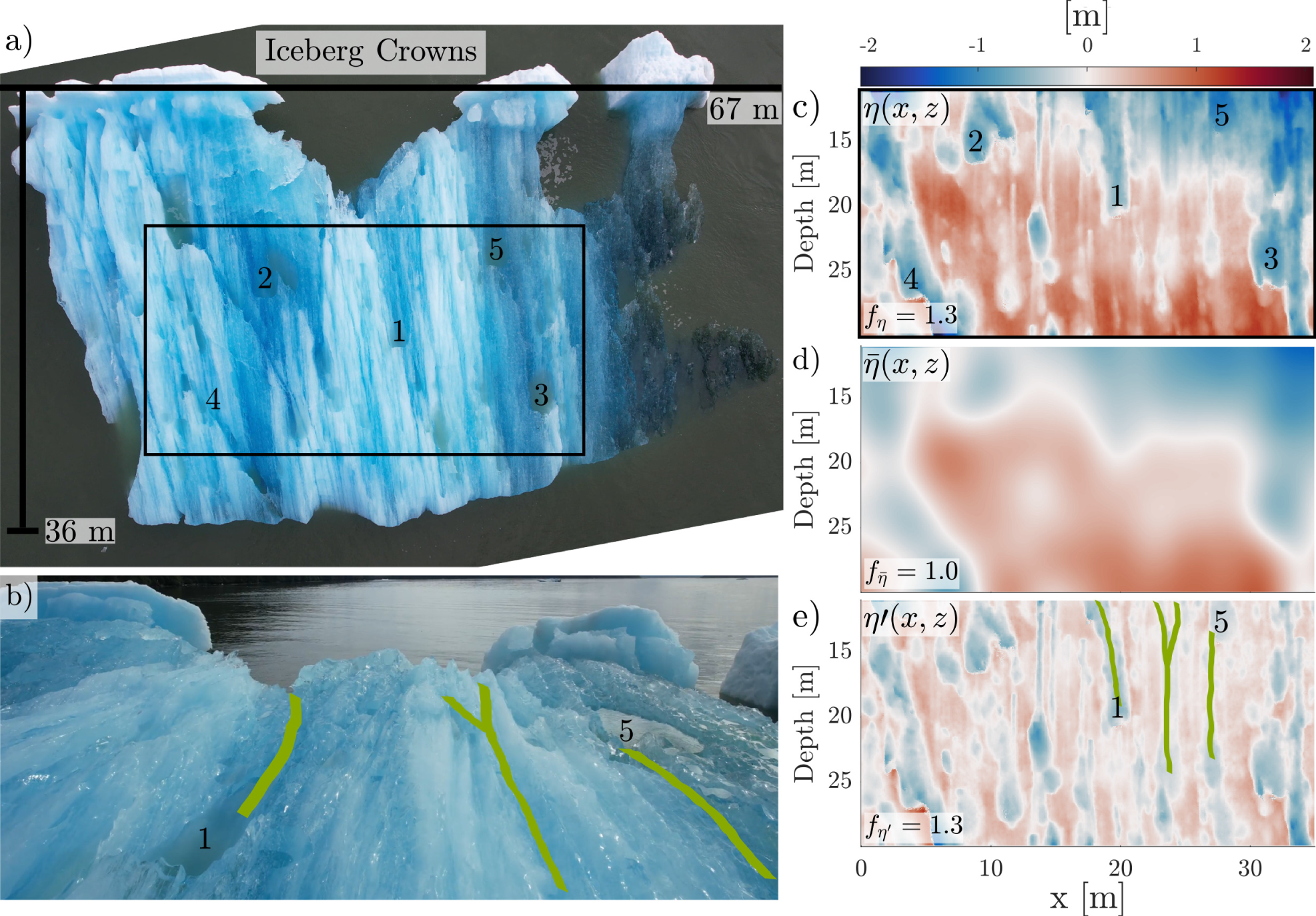
The side of the drone surveyed floating iceberg, named Queenofheartsberg, measures  $\sim67$ m in width ( $x$) and $\sim36$ m in depth ( $z$). The exposed ‘crowns’, the former above-water portion, extended roughly 5 m above the waterline (Fig. 6a). The formerly submerged face exhibits alternating dark and light blue layers, which had been oriented vertically underwater (Fig. 6a). A continuous subregion of the SfM-derived point cloud, 34.95 m by 29.95 m in size, was extracted to generate surfaces $\eta(x,z)$, $\bar{\eta}(x,z)$ and $\eta\prime(x,z)$ (Fig. 6c–e). The maximum relief of $\eta(x,z)$ reaches 2.07 m. The overall surface is relatively flat (Fig. 6d), but distinct features such as channels, crevasses and divots are present in both the relief maps and drone imagery. Markers 1–5 indicate matching features across both datasets (Fig. 6a, b, c, e). On a medium- to small-scale, the surface of this iceberg exhibits narrow channels that were vertically oriented when the face of this iceberg was still submerged (highlighted in green in Fig. 6b, e).
a) Optical drone image of Queenofheartsberg minutes after capsizing, exposing its submerged face. The image was rotated so the former above-water portion (‘crowns’) aligns with  $z=0$. The submerged face was $\sim36$ m deep and $\sim67$ m wide. b) Oblique drone view highlighting apparent channels (traced in green) and showing alternating dark and light blue ice layers that had been vertically oriented underwater. c–e) Relief maps of the iceberg surface: c) $\eta(x,z)$, d) $\bar{\eta}(x,z)$, e) $\eta\prime(x,z)$, derived from a 34.95 m by 29.95 m subregion of the SfM point cloud gridded at 5 cm resolution. The color scale represents surface relief and ranges from –2 m (blue) to +2 m (red) relative to the best-fit plane. Markers 1–5 and green lines indicate features visible in both images and relief maps.

2D slope spectral analysis and rugosity
A 2D slope spectral analysis of 55 iceberg side surfaces reveals how iceberg-scale morphology and medium- to small-scale roughness contribute differently to total ice–ocean interface area (Fig. 7). Of these, 40 surfaces exhibited narrowband roughness and could be decomposed into iceberg-scale and medium- to small-scale components. The remaining 15 surfaces displayed broadband roughness with no clear spectral peak; for these, only total rugosity ( $f_{\eta}$) could be calculated, which ranged from 1.1 to 2.0. Iceberg-scale and medium- to small-scale contributions could not be determined for these broadband surfaces.
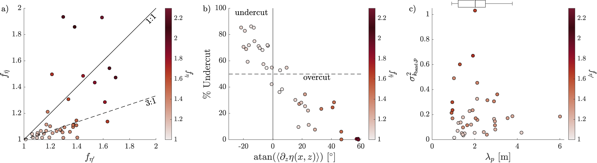
a) Scatter plot of medium- to small-scale rugosity ( $f_{\eta\prime}$) versus iceberg-scale rugosity ( $f_{\bar{\eta}}$), with points colored by total rugosity ( $f_{\eta}$). A solid black line indicates the 1:1 reference, and a dashed black line represents a 3:1 reference. b) Scatter plot of mean vertical slope ( $\text{atan}(\langle\partial_z\eta(x,z) \rangle)$) expressed as an angle versus the percentage of the surface that is undercut, with points colored by iceberg-scale rugosity ( $f_{\bar{\eta}}$). The solid vertical black line denotes a mean slope of $0^\circ$, corresponding to a vertical surface. The horizontal dashed line marks 50% undercut, indicating an equal division between overcut and undercut areas. c) Scatter plot of peak wavelength ( $\lambda_p$) versus the associated slope variance ( $\sigma^2_{k_\text{band},p}$), with points colored by medium- to small-scale rugosity ( $f_{\eta\prime}$). The colorbar scale ranges from 1.0 to 2.3 in all subplots to allow direct comparison of rugosity values. A box plot is shown above the $x$-axis, depicting the distribution of $\lambda_p$ values weighted by their corresponding $\sigma^2_{k_\text{band},p}$. The box represents the interquartile range (25th–75th percentiles), the line indicates the median (2.0 m) and the whiskers extend to the minimum and maximum non-outlier values. Two outliers, at 4.2 m and 6.0 m, lie beyond the whiskers.

In most narrowband cases, medium- to small-scale rugosity ( $f_{\eta\prime}$) exceeds iceberg-scale rugosity ( $f_{\bar{\eta}}$), with total rugosity ( $f_{\eta}$) ranging from 1.1 to 2.3 (Fig. 7a). Iceberg-scale rugosity remains relatively low across various iceberg-scale morphologies, though some overcut surfaces exhibit higher values than undercut surfaces (Fig. 7b). Given the mean surface extents of $\sim$10 m in both x and z, the interpretable limits of peak wavelengths is constrained to 0.8-1.6 m on the lower end by the sonar resolution (20–40 cm; $\geq4$ points per wavelength) and $\sim$3–3.7 m on the upper end by the finite surface extent ( $\geq3$ wavelengths per extent). Within these limits, the largest contributions to medium- to small-scale and total rugosity come from surfaces with high slope variability at wavelengths between 0.9 m and 3.7 m.
Of the 40 surfaces with narrowband roughness, 28 exhibit one identifiable spectral peak, 11 exhibit two and the drone-derived surface exhibits three. The iceberg-scale rugosity ( $f_{\bar{\eta}}$) ranges from 1.0 to 1.9, while the medium- to small-scale rugosity ( $f_{\eta\prime}$) ranges from 1.0 to 1.7. Combined, these yield total rugosity values ( $f_{\eta}$) as high as 2.3 (Fig. 7a). Most surfaces fall below the 1:1 line, indicating that medium- to small-scale roughness contributes more to surface area than iceberg-scale morphology. In 20 cases, the contribution of medium- to small-scale roughness to total surface rugosity exceeds a 3:1 ratio. In some cases, high total rugosity values ( $f_{\eta} = 1.9$) reflect relatively large contributions from both the iceberg-scale ( $f_{\bar{\eta}} = 1.4$) and medium- to small-scale ( $f_{\eta'} = 1.5$) components, as seen in Fig. 5d where the surface is steeply overcut with distinct channeling throughout. Other surfaces, such as Fig. 5g, exhibit more moderate total rugosity ( $f_{\eta} = 1.5$), with a lower iceberg-scale rugosity ( $f_{\bar{\eta}} = 1.2$) corresponding to a gently overcut morphology, but relatively higher medium- to small-scale rugosity ( $f_{\eta'} = 1.4$) associated with deep, slanted channels. In contrast, smoother examples like Fig. 5h display low total rugosity ( $f_{\eta} = 1.1$), with little contribution from either iceberg-scale ( $f_{\bar{\eta}} = 1.0$) or medium- to small-scale ( $f_{\eta'} = 1.1$) roughness.
At the iceberg scale, surfaces are classified as overcut if their mean slope is greater than  $0^\circ$ and less than 50% of the surface is considered undercut (lower right quadrant in Fig. 7b). Conversely, undercut surfaces have a mean slope less than $0^\circ$ and more than 50% of the surface is considered undercut (upper left quadrant in Fig. 7b). The mean slope refers to the mean vertical gradient of a surface from shallowest to deepest measurement depth. The observed mean slopes range from $-22^\circ$ to $58^\circ$ (Fig. 7b). Percent undercut refers to the percentage of grid cells where the vertical spatial gradient (Fig. 3c) of a surface is negative. The observed percent undercut metric ranges from 0% to 86% (Fig. 7b). Among the 40 surfaces identified as having narrowband roughness, 13 are classified as undercut, 19 as overcut and 3 as near-vertical (quadrants 2 and 3 in Fig. 7b). The drone-derived surface, collected above water, is not classified because the undercut metric requires subsurface measurements of vertical gradients. Despite the wide range in mean slopes and undercut percentages, these bulk iceberg properties show no clear relationship with rugosity (color of points in Fig. 7b). Only four surfaces exhibit iceberg-scale rugosity values above 1.3, all of which are classified as overcut.
Surfaces with the highest medium- to small-scale rugosity ( $f_{\eta'}$; color scale in Fig. 7c) are those where slope variance ( $\sigma^2_{k_\text{band},p}$; $y$-axis in Fig. 7c) is concentrated at particular wavelengths ( $\lambda_p$; $x$-axis in Fig. 7c). This indicates that rugosity is closely associated with enhanced slope variance at specific length scales. Based on this relationship between wavelength-dependent slope variance and surface area, a representative roughness length scale range is defined as the range of wavelengths associated with high slope variance: $0.9\text{\,m} \leq \lambda \leq 3.7\text{\,m}$. Across all surfaces, 53 peaks are identified, with wavelengths ranging from 0.7 m to 6.0 m. The dominant peak wavelength ( $\lambda_p$), defined as the peak with the highest $\sigma^2_{k_\text{band},p}$, ranges from 0.9 m to 6.0 m (Fig. 7c). A variance-weighted distribution of $\lambda_p$ values shows that 50% fall between 1.3 m and 2.4 m, with a median of 2.0 m (box plot in Fig. 7c). Two outliers occur at 4.2 m and 6.0 m.
Roughness statistics
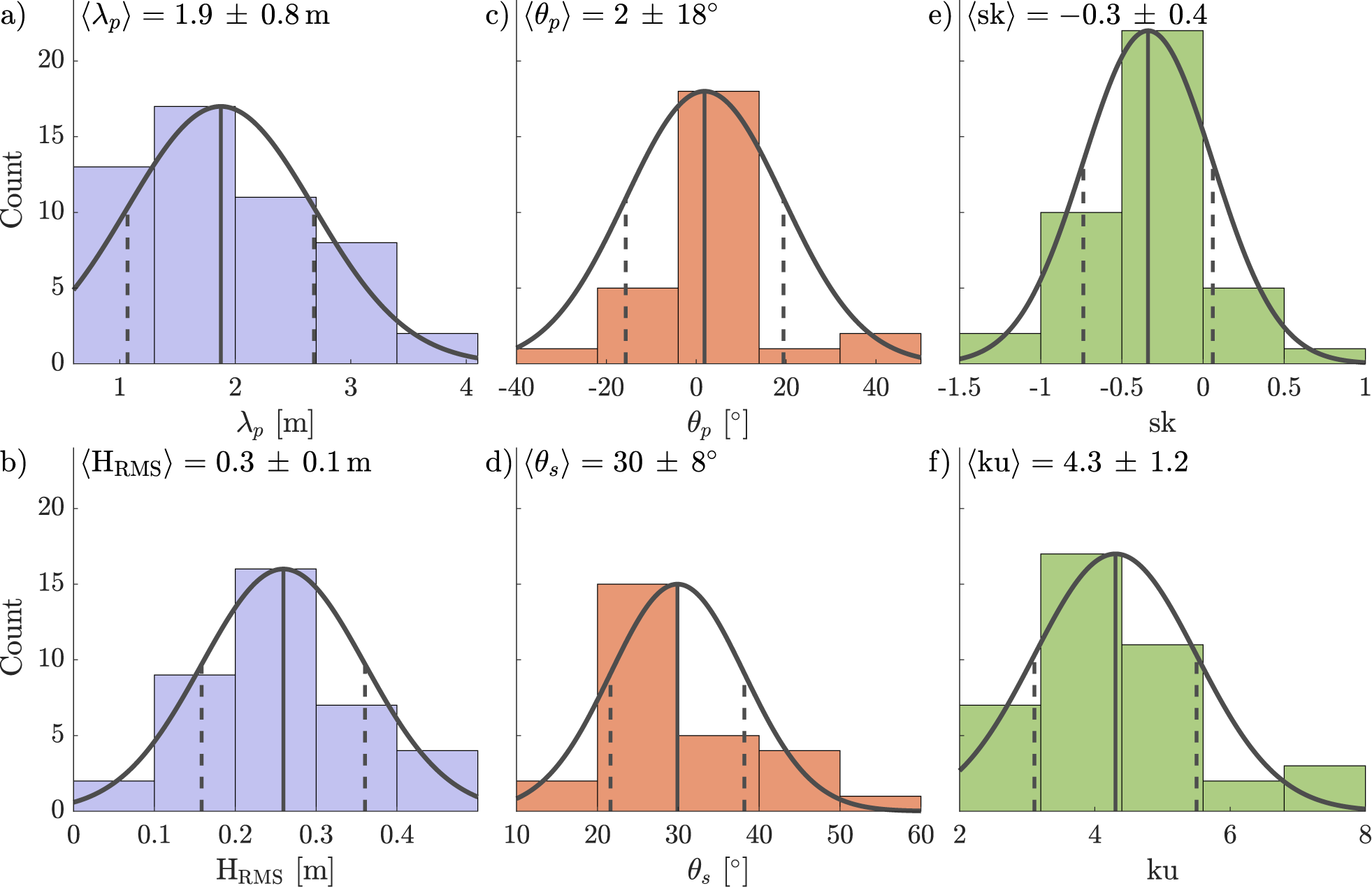
Roughness measurements from 38 surfaces fall within the defined roughness length scale (Fig. 8a, b). Across these surfaces, the mean emergent wavelength is  $1.9\pm0.8$ m, occurring well within the resolvable wavelength range of 0.9–3.7 m defined by sonar resolution and surface extent. The mean RMS height is $0.3\pm0.1$ m. Of the 38 surfaces, 27 are classified as anisotropic (Fig. 8c, d). The mean peak orientation for these anisotropic surfaces is $2\pm18^\circ$ (i.e., close to vertical). The associated directional spread averages $30\pm8^\circ$, indicating moderate to broad orientation spreading. PDFs of the rough surfaces ( $\eta\prime(x,z)$) yield a mean skewness of $-0.3\pm0.4$ and a kurtosis of $4.3\pm1.2$ (Fig. 8e, f), indicating moderately negatively skewed and leptokurtic surface relief distributions. For the drone-derived surface, three wavelength peaks are identified at 2.6 m, 1.0 m and 0.7 m. The RMS height associated with the rough surface is 0.2 m and skewness and kurtosis values of $-0.5$ and $4.9$, respectively, also indicating a moderately negatively skewed, leptokurtic distribution. The drone-derived surface is also classified as anisotropic, with a peak orientation of $0^\circ$ and a directional spread of $24^\circ$.
a)-f) Histograms showing the distributions of roughness statistics: a) peak wavelengths ( $\lambda_{p}$ [m]), b) RMS heights ( $\text{H}_\text{RMS}$ [m]), c) peak orientations for anisotropic roughness ( $\theta_{p}$ [ $^\circ$]), d) directional spread of anisotropic roughness ( $\theta_{s}$ [ $^\circ$]), e) skewness ( $\mathrm{sk}$) and f) kurtosis ( $\mathrm{ku}$). Grey curves represent Gaussian fits scaled to the histogram peak for visual comparison. Solid vertical lines indicate the mean value, while dashed vertical lines mark one standard deviation from the mean. Blue and orange histograms display statistics derived from 2D spectral analysis, while green histograms represent statistics obtained from PDF analysis.

Discussion
Synthesis of observations of ice roughness and iceberg-scale morphology
We present observations of submarine roughness at icebergs, a factor not commonly resolved or explicitly included in most ice melt models, despite evidence that it can influence melt rates (Watkins and others, Reference Watkins, Bassis and Thouless2021). The fine-resolution gridded surfaces of the ice–ocean boundary reveal that iceberg morphology over a  $\sim$10 m extent in $x$ and $z$ is dominated by near-vertical channels with wavelengths ranging between 0.9 m and 3.7 m, superimposed on larger-scale iceberg morphology. Most of the sonar-derived surfaces, along with the drone-derived surface, were characterized by narrowband roughness and were therefore included in the roughness decomposition and statistical analysis, while the smaller subset of broadband cases was retained only for total rugosity estimates ( $f_\eta=1.1–2.0$, mean $1.4 \pm 0.3$) but excluded from further scale-specific decomposition. For the narrowband surfaces, our statistical analysis suggests that submarine ice roughness is best described by a peak wavelength of $1.9\pm0.8$ m, an RMS height of $0.3\pm0.1$ m, an orientation of $2\pm18^\circ$, a directional spread of $30\pm8^\circ$, a skewness of $-0.3\pm0.4$ and a kurtosis of $4.3\pm1.2$ (Fig. 8). The statistics from the drone-derived surface agree well with the mean statistics computed from all sonar-derived grounded iceberg surfaces.
Our observations show that, on average, medium- to small-scale ice roughness and iceberg-scale morphology contribute roughly equally to surface area increases, with mean rugosity of  $f_{\eta\prime} = 1.3 \pm 0.2$ compared to $f_{\bar{\eta}} = 1.2 \pm 0.3$ for iceberg-scale morphology. This contribution can increase the total ice–ocean boundary surface area by more than a factor of 2, with mean total rugosity of $f_{\eta} = 1.5 \pm 0.3$ and maxima as high as 2.3 (Fig. 7). In most cases, medium- to small-scale rugosity contributes more to total surface area than iceberg-scale morphology, and in half the cases it exceeds the iceberg-scale contribution by more than 3 times as much (Fig. 7a). While these results underscore the importance of medium- to small-scale roughness, iceberg-scale morphology also contributes to surface area, with values reaching up to 1.9 for the most overcut surfaces (Fig. 7b). Broadband surfaces, although they could not be decomposed into iceberg-scale and roughness components due to the absence of a discernible peak in the slope-variance distribution, exhibited total rugosity values comparable to the narrowband cases. This similarity suggests that even when a distinct spectral peak is absent, broadband surfaces still contribute meaningfully to overall increases in ice–ocean boundary area. Together, these results emphasize that both roughness scales and, in some cases, broadband variability can be important to total surface area increases.
Of the 38 surfaces exhibiting narrowband roughness, 27 were classified as anisotropic, with a mean peak orientation of  $2\pm18^\circ$ and a directional spread of $30\pm8^\circ$ (Fig. 8c, d). This anisotropy suggests a dominant directional turbulent flow, aligned with gravity, at the ice–ocean boundary. The icebergs surveyed in this study were located approximately 15 km from the glacier where they originated. Based on observations of an iceberg traveling down the fjord during one of our campaigns, as well as input from a local tour operator, we estimate that it takes about 4–5 days for an iceberg to cover this distance. Considering this transit time and estimated melt rates for icebergs in the fjord ranging from 0.5–1.5 m day $^{-1}$ (Weiss and others, Reference Weiss2025), we infer that the iceberg faces we imaged were not the original calving surfaces. Instead, these faces were likely modified by melting during transit.
Roughness in melt predictions
Studies using remotely sensed, area-averaged submarine melt measurements have reported discrepancies between observed and predicted melt rates, with observations exceeding model predictions (Sutherland and others, Reference Sutherland2019; Schild and others, Reference Schild, Sutherland, Elosegui and Duncan2021). These studies noted that sub-grid scale features could partly explain such discrepancies. For example, Sutherland and others (Reference Sutherland2019) quantified a  $\sim$1.5 $\times$ increase in total surface area compared to a flat planar surface at Xeitl Sít’, while Schild and others (Reference Schild, Sutherland, Elosegui and Duncan2021) used drone and sonar data to reveal substantial differences in above- and below-water iceberg morphology of floating icebergs in Greenland. Schild and others (Reference Schild, Sutherland, Elosegui and Duncan2021) further showed that simplified geometric assumptions underestimated the total iceberg surface area by up to 43%, which in turn caused melt rates, when inferred from surface lowering measurements, to be overestimated. However, both studies were limited by the spatial resolution of the available data and could not fully resolve sub-meter roughness features.
If existing models of near-vertical ice boundaries incorporate medium- to small-scale roughness elements similar to our observations, a cross-flow along-ice ocean boundary current would encounter roughness features oriented perpendicular to the flow direction. Studies in non-ice contexts have shown that roughness significantly impacts boundary turbulence (Coceal and others, Reference Coceal, Dobre, Thomas and Belcher2007; Kadivar and others, Reference Kadivar, Tormey and McGranaghan2021) and that specific surface characteristics, such as surfaces with negative skewness (Flack and others, Reference Flack, Schultz and Volino2020), influence surface drag. The effect of roughness geometry and length scale on boundary-layer turbulence and drag is directly relevant to ice–ocean models, where the drag coefficient governs momentum transfer and melt rates. Therefore, inaccuracies in how roughness is represented within standard melt theory (McPhee and others, Reference McPhee, Maykut and Morison1987; Holland and Jenkins, Reference Holland and Jenkins1999; Jenkins, Reference Jenkins2011; Jackson and others, Reference Jackson2017) can lead to significant errors in melt rate predictions (Gwyther and others, Reference Gwyther, Galton-Fenzi, Dinniman, Roberts and Hunter2015).
Results from this study show that the ice surface can have 2.2 $\times$ more surface area than a flat wall geometry, which is often used in numerical simulations (Gayen and others, Reference Gayen, Griffiths and Kerr2016). Our field observation of increased surface area of the ice face highlights the need to account for both roughness and iceberg-scale morphology in ice–ocean melt models. The spectral approach used here provides a scale-resolved way to quantify roughness, highlighting the need to incorporate length-scale dependent morphology into ice–ocean melt models. Implementation of real ice geometries may improve ice melt rate predictions. Evolving ice boundaries have been explored using various modeling approaches, including 2D fine-resolution phase-field models (Hester and others, Reference Hester, Couston, Favier, Burns and Vasil2020), direct numerical simulations (DNS) of ice melting in freshwater (Yang and others, Reference Yang, Chong, Liu, Verzicco and Lohse2022), DNS of an ice layer over a turbulent stream of warm water (Perissutti and others, Reference Perissutti, Marchioli and Soldati2024) and limited-resolution 3D phase-field models (Couston and others, Reference Couston, Hester, Favier, Taylor, Holland and Jenkins2021) for larger scales. Phase-field models simulate melting and freezing by smoothing the ice–water interface and solving coupled equations for fluid flow and heat transfer. These models have shown that melt-driven topography such as scallops and channels can evolve under different flow conditions, with larger-scale 3D simulations suggesting that channels aligned with the flow can enhance local melt rates (Couston and others, Reference Couston, Hester, Favier, Taylor, Holland and Jenkins2021). However, no modeling studies have yet investigated the implications of roughness features of medium- to small-scales $\mathcal{O}$(0.5–5 m) at near-vertical ice–ocean boundaries.
Presence of channels as evidence for melt-driven morphological features
Understanding how oceanic conditions shape ice—ocean boundary morphology is key to understanding ice–melt processes. Laboratory experiments demonstrate how the interplay of flow dynamics and temperature conditions can produce distinctive patterns such as ice scallops (Bushuk and others, Reference Bushuk, Holland, Stanton, Stern and Gray2019; Sweetman and others, Reference Sweetman, Shakespeare, Stewart and McConnochie2024). Ice scallops have been shown to result from feedback between surface geometry and turbulent flow, where recirculating eddies within scallop troughs drive differential melt rates that stabilize their geometry (Bushuk and others, Reference Bushuk, Holland, Stanton, Stern and Gray2019). Temperature further influences scallop formation and growth: higher temperatures promote larger, asymmetric scallops due to intensified turbulent mixing, while lower temperatures favor smaller, more symmetric forms (Sweetman and others, Reference Sweetman, Shakespeare, Stewart and McConnochie2024). Together, these findings highlight the complex interplay between ice morphology and turbulent fluxes at the ice–ocean boundary.
At ice–ocean boundaries, buoyancy production from melting has contrasting effects depending on the orientation of the boundary. For near-horizontal surfaces, such as the base of sea ice, buoyancy suppresses turbulence in the boundary layer (McPhee and others, Reference McPhee, Maykut and Morison1987; Rosevear and others, Reference Rosevear, Gayen, Vreugdenhil and Galton-Fenzi2025). In contrast, near-vertical boundaries, such as those of marine-terminating glaciers and icebergs, produce buoyant meltwater plumes as freshwater rises along the ice face (Wells and Worster, Reference Wells and Worster2008; Gayen and others, Reference Gayen, Griffiths and Kerr2016; Parker and others, Reference Parker, Burridge, Partridge and Linden2021). This behavior, described as a ‘distributed wall-source plume’ (Parker and others, Reference Parker, Burridge, Partridge and Linden2021), transports meltwater away from the ice as meltwater intrusions (Jackson and others, Reference Jackson2020; Parker and others, Reference Parker, Burridge, Partridge and Linden2021). Buoyancy and shear production can generate turbulence that modulates melting at the boundary (Nash and others, Reference Nash2024).
Our observations show consistent vertical channeling across three separate field campaigns, along with high melt rates on iceberg faces. Together, these observations support the hypothesis that buoyancy-driven meltwater plumes play a key role in shaping near-vertical ice–ocean boundaries. Although the average peak orientation is  $2\pm18^\circ$, not all surface features are vertically aligned. The high variability in peak orientation and a directional spread of $30\pm8^\circ$, which suggests moderate to broad directional spreading (Fig. 8c, d), may stem from several factors. Non-uniform melting on different sides of an iceberg could induce tilting. Tidal exchanges acting on grounded icebergs may cause additional tilting and generate strong horizontal currents, measured at 0.02–0.12 m s $^{-1}$ at floating icebergs in this area (Weiss and others, Reference Weiss2025). If tilting occurred shortly before imaging, channels initially aligned with gravity would appear slanted. Moreover, grounded icebergs, which are more affected by horizontal currents, may show distorted channel orientations compared to floating icebergs. Recent DNS results by Perissutti and others (Reference Perissutti, Marchioli and Soldati2024) further suggest that flow strength can control the emergence of roughness orientations, with weaker flows producing streamwise features and stronger flows producing spanwise features.
The contrast between broadband and narrowband surfaces may also reflect differences in the dominant melt regime. Whereas narrowband cases are characterized by distinct channels aligned with a preferred wavelength, broadband cases lack this organization and may instead represent diffuse, spatially distributed melt without strong channelization. This interpretation suggests that different roughening mechanisms, buoyancy-driven channel formation versus shear driven melt, may leave distinct spectral signatures on iceberg faces. Variability may therefore arise from the combined influence of buoyant plume-driven currents, which tend to enhance vertical channeling, and horizontal shear flows, which may disrupt or mask channelization and produce more diffuse broadband signatures. Queenofheartsberg, the only floating iceberg, was likely more affected by vertical plume-driven currents than horizontal flows, as evidenced by its narrower directional spread of  $24^\circ$ and peak orientation of $0^\circ$.
Icebergs in this study were surrounded by relatively warm, stratified waters (3–10  $^\circ$C, 23–28 psu) and melted at rates of 0.5–1.5 m day $^{-1}$ (Weiss and others, Reference Weiss2025), which are higher than typical melt rates near Greenland (Schild and others, Reference Schild, Sutherland, Elosegui and Duncan2021) or Antarctica (Stanton and others, Reference Stanton2013). These conditions likely enhanced plume activity and melt-driven shaping of the ice. Thus, the statistics presented here may be biased toward these elevated melt conditions. However, under Antarctic ice shelves, the pressure melting point is depressed at depth, allowing basal melt to occur even in colder waters, particularly where warm deep water intrudes (e.g., Rignot and others, Reference Rignot, Jacobs, Mouginot and Scheuchl2013; Stanton and others, Reference Stanton2013; Alley and others, Reference Alley, Scambos, Siegfried and Fricker2016). This suggests that pressure-related melting may also contribute to roughness formation in colder environments. Further studies are needed to understand whether similar channeling occurs in colder, less stratified regions.
Pathway toward incorporating realistic roughness statistics in ice–ocean melt models
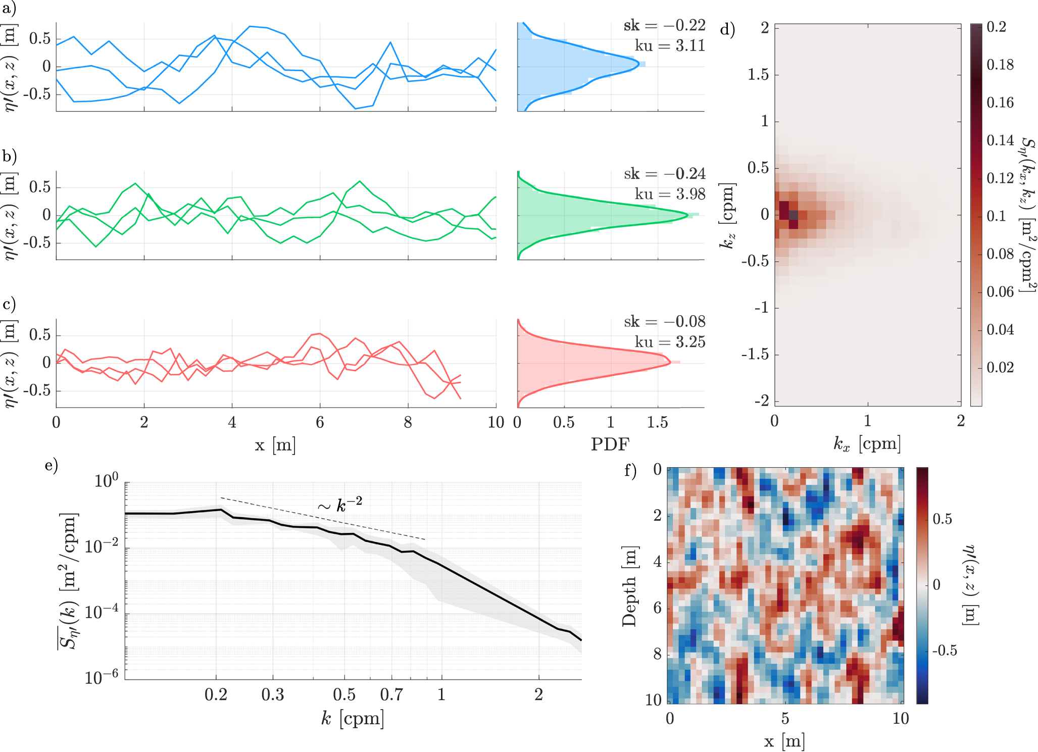
To support the integration of observed ice–ocean boundary characteristics into melt models, we present a conceptual framework for idealizing roughness statistics for use in model geometries (Fig. 9). Based on mean observations, we construct simplified 1D and 2D representations of iceberg surfaces that reflect key morphological features identified in this study. Figure 9a–c shows 1D profiles of along-ice ( $x$) surface relief ( $\eta\prime(x)$), selected to represent the mean skewness ( $\langle \mathrm{sk} \rangle = -0.3 \pm 0.4$) and kurtosis ( $\langle \mathrm{ku} \rangle = 4.3 \pm 1.2$) of all surfaces analyzed. Each profile is paired with its PDF for the entire surface, annotated with the corresponding $\mathrm{sk}$ and $\mathrm{ku}$ values. Figure 9d displays the mean 2D amplitude PSD, $S_{\eta\prime}(k_x,k_z)$, computed by averaging PSDs from surfaces with peak orientations within $\langle \theta_p \rangle = 2\pm 18^\circ$ and directional spreads within $\langle \theta_s \rangle = 30\pm 8^\circ$. The azimuthally averaged 1D amplitude spectrum from this mean PSD is plotted in Fig. 9e, showing a slope of approximately $k^{-2}$ across the medium- to small-scale roughness length scales explored in this study. Figure 9f shows a synthetic 2D iceberg surface ( $10\text{\,m} \times 10\text{\,m}$) generated from the mean PSD by assigning independent random phases drawn from a uniform distribution on $[0,2\pi)$ to each Fourier mode and applying an inverse 2D Fourier transform, and then taking the real part of the resulting field. This method produces a statistically representative and spatially coherent realization of the observed anisotropic roughness, capturing the mean peak wavelength and RMS height, along with their variability. These idealized schematics, grounded in observations, provide a framework for incorporating realistic boundary morphology into future ice–ocean models aimed at improving melt rate predictions.
Statistical and spectral representation of ice–ocean boundary roughness based on observations. a–c) 1D surface profiles of  $\eta\prime(x)$ extracted from observed surfaces a-ii, b-ii and c-ii in Figure 5. These profiles were selected because their skewness ( $sk$) and kurtosis ( $ku$) values fall within $\langle \mathrm{sk} \rangle = -0.3\pm0.4$ and $\langle \mathrm{ku} \rangle = 4.3\pm1.2$, respectively. Each profile is paired with its corresponding probability density function (PDF) of surface relief (right), annotated with the $sk$ and $ku$ values for that surface. d) Mean 2D amplitude PSD, $S_{\eta\prime}(k_x, k_z)$, computed by averaging PSDs from surfaces with peak orientations within $\langle \theta_p \rangle = 2\pm 18^\circ$ and directional spreads within $\langle \theta_s \rangle = 30\pm 8^\circ$. e) Azimuthally averaged 1D amplitude spectrum derived from panel d, plotted as a function of radial wavenumber $k$, with a reference slope of $k^{-2}$ overlaid for comparison. f) $10\times10$ m idealized iceberg surface characterized by the mean spectral properties and directional variability observed in this study. This surface was generated from the mean 2D amplitude PSD shown in panel d by assigning independent random phases drawn from a uniform distribution on $[0,2\pi)$ to each Fourier mode and applying an inverse 2D Fourier transform to produce a synthetic but statistically representative realization of anisotropic roughness.

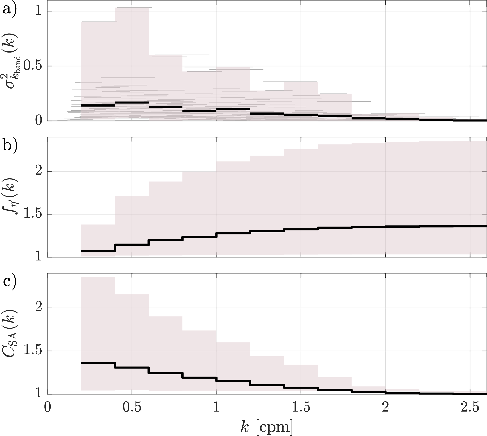
To further characterize the scale-dependent structure of ice roughness and inform its incorporation into model boundary conditions, we suggest a pathway for artificially increasing the ice surface area available for melt in numerical models that can only resolve a finite roughness length scale. To begin, we computed the mean slope variance spectra across all anisotropic surfaces (Fig. 10). Individual surfaces show broadly consistent spectral structure, with a peak in slope variance centered around 0.5 cpm (corresponding to a wavelength of  $\sim$2 m). The black line in Fig. 10a represents the mean slope variance as a function of wavenumber band, while the pink shaded region denotes the full range of values (minimum to maximum) observed across the dataset. The cumulative medium- to small-scale rugosity is computed by cumulatively summing the mean slope variance across wavenumber bands, $f_{\eta'}(k) \approx \sqrt{1 + \sum_{{k'\leq k}} \overline{\sigma^2_{k_\mathrm{band}}}(k')}$, as shown in Fig. 10b. This expression provides an approximation of rugosity based on slope variance. The resulting curve describes how the ice surface area increases with the inclusion of progressively finer-scale roughness. Conversely, Fig. 10c shows a correction factor $C_{\mathrm{SA}}(k)$ required to account for unresolved fine-scale features if only roughness larger than a given wavelength is captured or resolved. The correction factor is largest when only coarser features (low $k$) are resolved, as higher $k$ are resolved the correction factor decreases. The shaded pink area shows the spread between minimum and maximum observed roughness and reflects the natural variability in roughness across ice surfaces. The correction factor is meant to provide a pathway for modeling studies to statistically capture the full ice medium- to small-scale rugosity even if their model can only resolve low wavenumbers. If a model resolves only low wave numbers, the correction factor could be used to artificially increase the surface area of the model surface to then capture actual ice surface area available for melt as observed on icebergs in this study. Together, these results provide a possible way for idealizing subgrid-scale roughness and quantifying its impact on modeled ice–ocean fluxes.
a) Slope variance ( $\sigma^2_{k_\mathrm{band}}$) for individual surfaces (gray lines) plotted as horizontal bars across each wavenumber band. The bold black line represents the mean slope variance ( $\overline{\sigma^2_{k_\mathrm{band}}}$), and the pink shaded region denotes the full range (minimum to maximum) of binned mean slope variance values across all surfaces. The limits of $k$ were set by the range of length scales resolvable across all surfaces based on sampling limitations; the lower bound was determined by the longest wavelength that spanned the surface, limited by the surface dimensions and the upper bound was determined by the finest wavelengths resolvable due to surface gridding. Wavelength band widths were defined by averaging the resolvable bandwidths across all surfaces to provide a consistent spectral resolution. b) Cumulative medium- to small-scale rugosity $f_{\eta'}(k) \approx \sqrt{1 + \sum_{{k'\leq k}} \overline{\sigma^2_{k_\mathrm{band}}}(k')}$ as a function of wavenumber, where the summation represents the cumulative sum of the mean slope variance across all wavenumber bands up to $k$. This shows how the total surface area available for melt increases progressively as additional roughness scales are included. c) Surface area correction factor $C_{\mathrm{SA}}(k)$, indicating how much area is missed if only coarser features (low $k$) are resolved.

In addition to surface area corrections, many melt parameterizations that aim to resolve turbulent exchange at the ice–ocean boundary require specification of a roughness length scale, commonly denoted as  $z_0$ or in our coordinate system $y_0$, to estimate the friction velocity $u_*$ that governs momentum and heat fluxes within the boundary layer. The roughness length $z_0$ represents the height at which the logarithmic velocity profile extrapolates to zero and is strongly influenced by the size and geometry of surface roughness elements (Kadivar and others, Reference Kadivar, Tormey and McGranaghan2021). In ice–ocean models, $z_0$ is often assumed or empirically tuned based on roughness type, yet remains poorly constrained for natural ice surfaces. Laboratory and field studies have shown that $z_0$ can be approximated as a fraction of the roughness height, typically ranging from one-tenth to one-thirtieth of the RMS height (Nikuradse, Reference Nikuradse1950; Perry and others, Reference Perry, Schofield and Joubert1969; Jiménez, Reference Jiménez2004). Based on observations from this study, specifically RMS heights of $0.3\pm0.1$ m, we suggest that a first-order, physically grounded estimate for $z_0$ lies between $0.01-0.03 {\textrm{m}}$. This range corresponds to surfaces in the transitionally rough regime, where roughness begins to significantly disrupt the near-wall flow and enhance turbulent mixing (Kadivar and others, Reference Kadivar, Tormey and McGranaghan2021). As shown in prior work (Flack and Schultz, Reference Flack and Schultz2010), accounting for the geometric influence on $z_0$ is crucial for accurately predicting the friction velocity and the exchange of fluxes. While further research is needed to fully link ice specific topography with appropriate drag coefficients, our field-based estimates offer a practical foundation for incorporating a realistic subgrid-scale roughness length scale into iceberg-scale melt models.
Uncertainty in statistics
The maximum mean undercut surface observed in the study was  $-22^\circ$, while the maximum mean overcut surface was $58^\circ$, illustrating the significant range of slope variability and the challenge in equally quantifying both undercut and overcut regions (Fig. 7b). Although iceberg-scale measurements reveal a wide range of mean slopes and percent undercut, no clear relationship emerged between these bulk properties and medium- to small-scale roughness. Channel-like features appeared on both undercut and overcut surfaces, but roughness metrics did not exhibit clear differences between them. Frequent iceberg tilting, particularly for grounded icebergs affected by asymmetric melt or tidal forces, further complicates interpretation, as it may shift the apparent orientation of features away from their original iceberg-scale geometry. Thus, while no clear connection is evident, we cannot rule out a connection without better constraints on iceberg tilting during mapping.
Projection distortion was another challenge when mapping large-scale, non-planar morphologies and overlaying roughness features onto a regular grid (Friedman and others, Reference Friedman, Pizarro, Williams and Johnson-Roberson2012). In areas with shallow slopes or curvature, the wavelength of roughness features appeared compressed due to the projection method. While subdividing the iceberg side into smaller slope-consistent sections could have reduced distortion, it would have increased the minimum resolvable wavenumber during 2D spectral analysis. However, given the spatial scale of the iceberg surfaces ( $\sim10$ m) and the medium- to small-scale roughness wavelengths of interest (0.9–3.7 m), the effect of this distortion on wavenumber resolution is estimated to be less than 6%, corresponding to a potential compression of no more than 5–20 cm. This distortion is considered negligible because it falls below the lowest grid cell size used in surface generation (20 cm).
Another source of uncertainty arises from variability in spectral resolution across surfaces, which reflects differences in grid size and overall surface dimensions. Smaller surfaces with larger grid sizes had coarser spectral resolution, while larger surfaces with smaller grid sizes permitted finer resolution and detection of multiple peaks. For example, the drone-derived surface, which combined the largest surface area with the finest grid resolution, revealed multiple peaks that could not have been identified at coarser resolution. Standardizing bandwidths across all surfaces was not possible, as this would have required adopting the coarsest resolution, obscuring peaks in higher-resolution datasets. Instead, we applied the highest feasible resolution for each surface to maximize the ability to detect peaks. As a result, spectral bands were narrower in larger, finer-resolution surfaces and broader in smaller, coarser-resolution surfaces, leading to variation in the number and sharpness of peaks detected across the dataset.
Conclusion
This study provides the first fine-resolution observations of submarine roughness on iceberg surfaces, revealing ubiquitous, vertically aligned channelized features with wavelengths ranging from 0.9 m to 3.7 m and a characteristic peak around 1.8 m. These features were observed across multiple field campaigns and 15 km from the glacier where they originated, which suggests that local oceanographic conditions, rather than inherited calving geometries, dominate the formation of iceberg surface roughness. As the dominant features were oriented within  $2\pm18^\circ$ of vertical, we infer that they were likely shaped by plume-driven melting. However, the high variability in channel orientation and the moderate to broad spread in the anisotropy points to the influence of cross flows, tilting and iceberg motion in modifying melt-driven morphology.
While our measurements were made on icebergs downstream of the glacier terminus, they provide an accessible analog for studying near-vertical ice–ocean boundaries at field scale. Icebergs are subject to the same oceanic forcing and melt-driven processes that act at glacier termini, and thus capture how plume activity, shear and stratification shape ice roughness. Importantly, iceberg melt itself does not contribute to sea-level rise; rather, these observations are complementary to direct measurements at glacier fronts. They highlight fundamental ice–ocean interaction mechanisms that are likely also active at the terminus, while underscoring the need for future work directly at glacier boundaries to fully constrain their role in sea-level change.
A key contribution of this study is a spectral, scale-resolved approach for characterizing roughness, which identifies contributions from different length scales to overall iceberg roughness. Our results show that both medium- to small-scale roughness (0.9-3.7 m) and iceberg-scale morphology  $\mathcal{O}$(10 m) can significantly increase the total ice–ocean boundary surface area, by up to factors of 1.7 and 1.9, respectively, relative to a flat reference plane. This enhanced rugosity has two important implications for melt modeling. First, increased surface area provides more interface for heat exchange, potentially increasing total melt. Second, roughness elements can modify turbulence and momentum transfer at the boundary, affecting melt rates through changes in boundary layer dynamics. Our findings highlight a critical gap in current melt models, which often neglect roughness at the observed spatial scales. We provide a pathway for incorporating both the increased surface area available for melt due to medium- to small-scale ice roughness in each wavenumber, as well as a statistic for incorporating a realistic roughness length scale $z_0$ when estimating shear applied to the boundary within melt models. Incorporating these morphological features at near-vertical ice–ocean boundaries has the potential to improve melt predictions and may help reconcile discrepancies between observed and modeled melt rates reported in previous studies. The influence of iceberg-scale morphology on medium- to small-scale roughness remains uncertain. Future work will aim to identify dependencies between large-, intermediate- and small-scale features at larger icebergs in Xeitl Geeyi’ and at the glacier Xeitl Sít’.
Supplementary material
The supplementary material for this article can be found at https://doi.org/10.1017/jog.2026.10135.
Acknowledgements
Funding was provided by the National Science Foundation (OPP-2023674), the Keck Foundation (2021-698) and the Murdock Charitable Trust (2022-5149). We thank Scott and Julie Hursey, Lila and Grant Trask, the captain and crew of the RV Steadfast and the community of Petersburg, AK. We are also grateful to Nicole Abib, Lucy Wanzer, Bridget Ovall, Kaya Troyer, Leonardo Nolasco, Dan Duncan and Eli Hunter for their valuable discussions on submarine ice morphology and their assistance in the field. Finally, we acknowledge the Shatx’héen Kwáan Tlingits, whose ancestral lands lie in this region.



















 Open access

