2.1. Glacier–fjord system

We focus our study on the Hansbreen Glacier–Hansbukta Fjord system, which is a branch of the Hornsund fjord, located in Southern Spitsbergen, Svalbard, at ~77°N (Fig. 1).

Fig. 1.

Location of Hansbreen–Hansbukta, Svalbard (inset). ASTER image of Hansbreen–Hansbukta showing the location of the modeled flowline (red line) and the locations of the stakes for velocity measurements (colored circles). Only the velocity stakes marked with blue dots were used in our analysis. The white triangle indicates the position of the time-lapse camera. The axes include the UTM coordinates (m) for zone 33X.

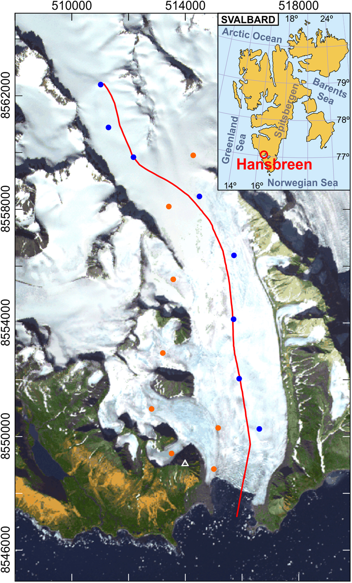
The Svalbard archipelago is of a particular interest because marine-terminating glaciers constitute 44% of its glacierized area (Pfeffer and others, Reference Pfeffer2014). Although in recent years its mass losses from glacier wastage have been the lowest of all Arctic regions (Gardner and others, Reference Gardner2013), these losses have been predicted to increase substantially to the end of the 21st century (Huss and Hock, Reference Huss and Hock2015; Lang and others, Reference Lang, Fettweis and Erpicum2015; Möller and others, Reference Möller, Navarro and Martín-Español2016).

Hansbreen is a tidewater glacier ~16 km long and 2.5 km wide. It has a 1.5 km-wide calving front, with a vertical face that is ~100 m thick at the central flowline, of which 50–60 m are submerged. The bed of the central flowline lies below sea level as far as 10 km up-glacier from the terminus, with the 4 km closest to the terminus overlying a reverse-slope bed (Fig. 2). Surface velocity increases toward the terminus, reaching values up to ~7 m week⁻¹. Velocities vary seasonally, reaching maxima during late spring–early summer. Iceberg calving usually starts in May and ends in October, and the mean annual calving rate is 250 m a⁻¹ (Blaszczyk and others, Reference Blaszczyk, Jania and Hagen2009).

Fig. 2.

Hansbreen–Hansbukta system model domain (left), and a detail of Hansbukta (right).

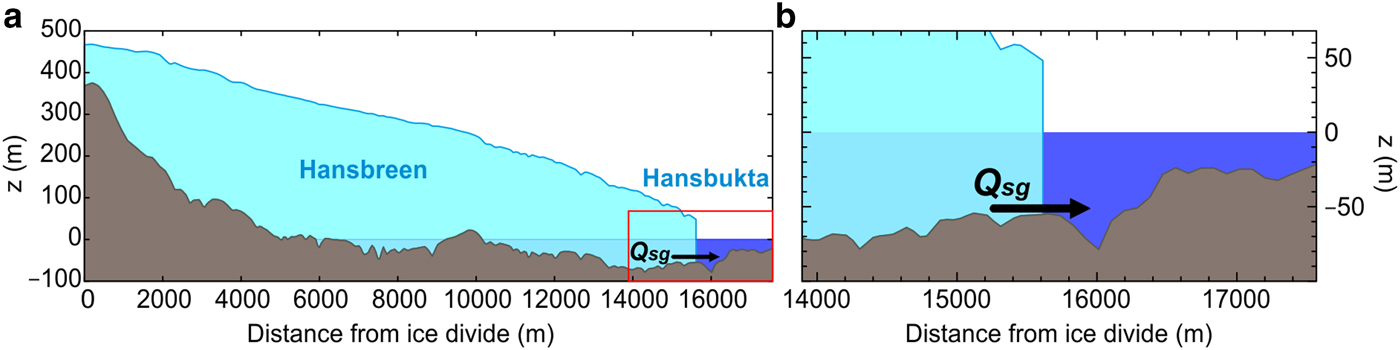
Hansbukta is Hansbreen's ~2 km-long proglacial fjord. It is a shallow fjord (<80 m depth), with a prominent and long sill of ~25 m depth that extends toward the fjord mouth (Fig. 2). Hornsund region is characterized by a relatively warm and humid climate due to the influence of the West Spitsbergen Current, which carries warm and salty Atlantic waters that mix with the fresher and cooler fjord waters during the summer season (Cottier and others, Reference Cottier2010; Walczowski and Piechura, Reference Walczowski and Piechura2011). The heat exchange taking place between water masses strongly influences submerged-ice melting.

2.2. Data

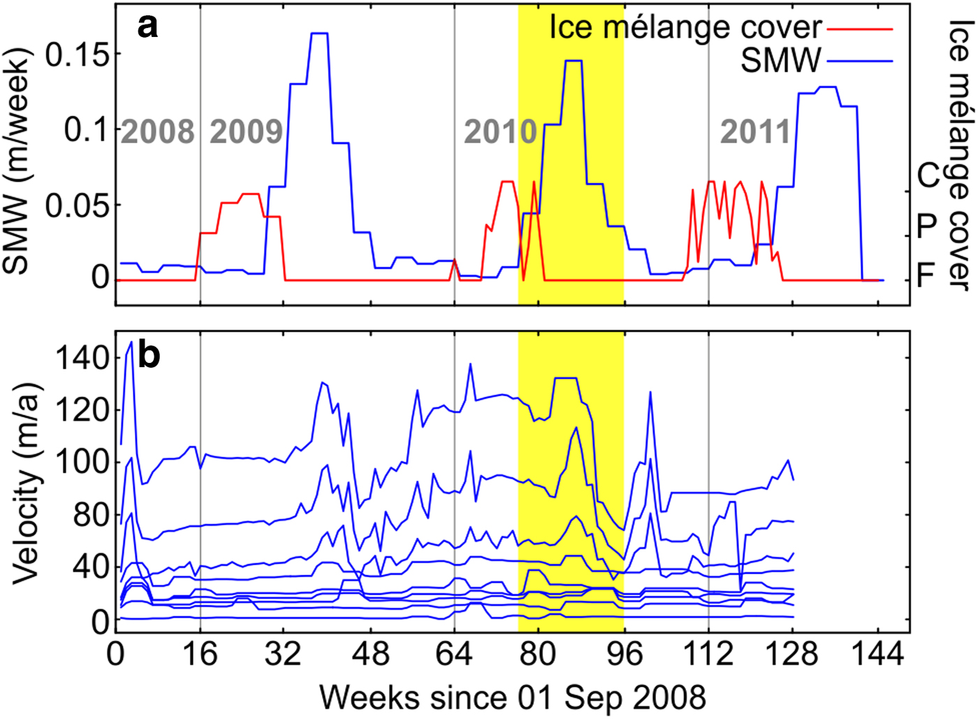
Observational constrains on the glacier model include surface velocities, front positions, ice-melánge coverage, surface elevation, bedrock topography and surface mass-balance (SMB) estimates. Ice surface velocities (Fig. 3a) were measured daily, from May 2005 to April 2011, at stakes located close to the flowline (Puczko, Reference Puczko2012) and from terrestrial laser scanner for the velocities at the glacier terminus (Otero and others, Reference Otero2017). Front position data and ice-mélange coverage from time-lapse camera images taken every 3 h (Fig. 3b) were processed and averaged over weekly intervals between December 2009 and September 2011 (Otero and others, Reference Otero2017). SMB was obtained from European Arctic Reanalysis (EAR) data, with 2 km horizontal resolution and hourly temporal resolution, constrained by automatic weather stations and stake observations (Finkelnburg, Reference Finkelnburg2013). First, ablation was calculated from the surface energy balance (SEB), which is resolved in the EAR by an optimized version of the unified NOAA Land Surface Model (Chen and Dudhia, Reference Chen and Dudhia2001) of the Polar WRF 3.4.1 model. The algorithm solving for the SEB takes into account net radiation, sensible heat flux, latent heat flux and heat flux across the glacier surface for glacierized areas and across the ground for non-glacierized areas, and encompasses all heat fluxes involved in melt and refreezing processes within the snowpack. Second, accumulation was obtained as the solid (frozen) precipitation of the Morrison bulk microphysics scheme for cloud physics used by the EAR. Finally, monthly mean SMB and SMW at each flowline point were calculated by applying bilinear interpolation to the available 2 km resolution hourly accumulation and ablation data (Fig. 3b). The surface elevation came from the SPIRIT Digital Elevation Model (DEM) for gentle slopes, with a 30 m root-mean-square absolute horizontal precision and 40 m resolution. Bedrock topography was inferred from ground-penetrating radar data (Grabiec and others, Reference Grabiec, Jania, Puczko, Kolondra and Budzik2012; Navarro and others, Reference Navarro2014).

Fig. 3.

Time evolution of: (a) sea–ice coverage (red) and surface meltwater estimations (blue); (b) surface velocities in Hansbreen. Velocities increase near the glacier front. The yellow region indicates the overlapping period when both glacier and fjord data are available (April to August of 2010).

Available oceanographic data overlap glaciological data only for 5 months, limiting our coupled modeling from April to August of 2010 (~20 weeks). During this period, several water temperature and salinity data sets were collected in Hansbukta (Fig. 4) using a SBE 19plus Conductivity-Temperature-Depth (CTD) probe, profiling with a frequency of 4 Hz with an initial accuracy of 0.0005 S m⁻¹ for conductivity, 0.005°C for temperature and 0.1% of full-scale range for pressure. All the data were vertically averaged every 1 dbar (1 kPa). From April to August, data gaps in temperature and salinity were linearly interpolated, maintaining the vertical structure of the water column (i.e. the interpolation was applied to each vertical level). The 2-D model domain of Hansbreen was extended into Hansbukta, using bathymetry linearly interpolated from depth soundings measured at irregular intervals of ~100 m (Vieli and others, Reference Vieli, Jania and Kolondra2002). Bathymetry varies from ~55 to 25 m depth (glacier front and sill, respectively), reaching the maximum depth of 79 m at ~200 to 400 m down-fjord from the glacier front (depending on glacier front position).

Fig. 4.

Map of CTD stations in Hansbukta, during the oceanographic surveys in spring–summer of 2010. The data of the stations with maximum depth, contained in the white ellipse close to the glacier front, were used to set the initial conditions. The stations inside the white circle farther away from the front were located on the sill, and their data were used to prescribe the boundary conditions. Data from all non-yellow CTD stations were used for comparison with model results. The panel to the right shows the time evolution of the observed temperature (T, upper panel) and salinity (S, lower panel) profiles set as initial (solid lines) and boundary (dotted lines) conditions. The temporal evolution is represented by colors as indicated by the legend for the CTD stations, and black lines represent profiles linearly interpolated in time.

3.1. Fjord circulation and submarine melt models

We use a simplified 2-D (x-z coordinates) model of water circulation inside the fjord, which includes a source of mass at the grounding point and oceanic forcing at the fjord mouth. Atmospheric forcing, waves, tides or ice-mélange melting are not considered in our present study. We use the Navier–Stokes set of equations for incompressible and stratified fluid in a non-rotating system (Coriolis effects can be neglected, since the Rossby number for the modeled system is ~10). The equations driving the fluid dynamics are conservation of mass (1), budget of momentum (2), heat (3) and salt (4). The model variables are: velocity vector $({\bf u})$, temperature (T), salinity (S) and pressure (p). To estimate the density of sea water (ρ) as a function of temperature and salinity, we use the non-linear equation of state of Jackett and Mcdougall (Reference Jackett and Mcdougall1995), setting the reference density as ρ ₀ = 1027 kg m⁻³. Assuming the Boussinesq approximation, where ρ = ρ ₀ + ρ′(x, z, t), with |ρ′| ≪ ρ ₀, the governing equations take the form:

(1)$$\nabla \cdot {\bf u} = 0,$$

(2)$$\displaystyle{{\hbox{d}{\bf u}} \over {\hbox{d}t}} = {\bf g} - \displaystyle{1 \over {\rho _0}}\nabla p + A{\rm \;} \nabla ^2{\bf u},$$

(3)$$\displaystyle{{\hbox{d}T} \over {\hbox{d}t}} = K_{{\rm T\;}} \nabla ^2T,$$

(4)$$\displaystyle{{\hbox{d}S} \over {\hbox{d}t}} = K_{\rm S}{\rm \;} \nabla ^2S,$$

where ${\bf g}$ is the gravity acceleration vector, A is the kinematic viscous coefficient (Laplacian Eddy Viscosity, assumed to be horizontally and vertically invariant) and K _T,S are the thermal and haline diffusive coefficients. The 2-D configuration is a major simplification that does not allow the model to reproduce dynamical processes in the y-direction, which can be partially compensated by a proper choice of the viscous and diffusive coefficient values. Considering our aims of simulating both fjord circulation (with likely laminar flow regime) and buoyant plume at the glacier face (with potentially turbulent flow regime), the assumption that the viscous and diffusive coefficients are independent of position and velocity (both horizontally and vertically) is also a major simplification that might limit the capability to simulate turbulent flows embedded in stratified environments. The advantage of using a 2-D model is the capability of performing a large number of high-resolution simulations with reduced computational cost as compared with a 3-D model. By contrast, the 2-D fjord model represents a fjord where processes are assumed to be invariant in the y-direction, which is unlikely to happen in the real system. Key points of the real system not captured by the 2-D model are that discharge channels are not evenly distributed along the entire fjord width and that advective fluxes in the y-direction change the velocity fields and redistribute fjord water properties in a more complex way.

We use the Massachusetts Institute of Technology general circulation model (MITgcm; Marshall and others, Reference Marshall, Adcroft, Hill, Perelman and Heisey1997) to solve the non-hydrostatic form of the above equations on a generalized curvilinear grid, vertically fixed on z-levels. The finite-volume discretization follows the Arakawa C-grid (see Arakawa and Lamb, Reference Arakawa and Lamb1977) and we rendered it horizontally variable in the x-direction on a structured cell grid.

We set a 2-D fjord domain of ~2 km in length along the x-coordinate (extension of the glacier central flowline), varying according to changes in glacier-front position (Fig. 2). The mesh consisted of 200 × 90 cells (horizontal–vertical). To capture small-scale processes, we set a high-resolution x-zone of 1 m gridcell length for the 100 m closest to the glacier front, and then linearly increasing to the end of the domain. The gridcell height along the z-coordinate was fixed to 1 m. The model width in the y-direction is one gridcell of 1 m. Sensitivity analyses were performed to constrain the optimal values of the diffusion coefficients, based on best-fit salinity profiles inside the fjord (temperature was less sensitive). We used the run-time week 17 due to the warm temperatures of the fjord waters and to the salinity stratification at the top layer, which allowed us to compare the different patterns of modeled profiles resulting from different values of the diffusive coefficients. We tested values of K _T,S in the range from 10⁻³ to 10⁻¹ m² s⁻¹ with constant subglacial discharge velocities of 0.1 m s⁻¹, obtaining the best fit for values of K _T,S = 1.4 × 10⁻³  m² s⁻¹. We could assume that the flow is fully turbulent inside the buoyant plume and set heat and salt diffusivities equal to the kinematic eddy viscosity (McPhee and others, Reference McPhee, Maykut and Morison1987). However, this cannot be assumed for the circulation in the rest of the fjord, where one must distinguish between viscous and diffusive processes. Therefore, Laplacian viscosity (A _h,v) was set to 1.4  ×  10⁻² m² s⁻¹ to match the expected order of magnitude of the Prandtl number for sea water (10¹). We found the value of A to be consistent with previous studies for the same spatial resolution (Xu and others, Reference Xu, Rignot, Fenty, Menemenlis and Flexas2013). The top boundary of the domain (sea level) was considered as a free surface, while the bottom (seabed) was set as a closed boundary (no normal flux, no tracer gradients) following the observed bathymetry with no-slip conditions (no tangential movement). The left side of the domain (glacier front) was also considered as a permanently vertical closed boundary with no-slip conditions in the fjord model. The right side (the fjord mouth) was set as an open boundary with transient temperature and salinity profiles according to the observed oceanic forcing. A more detailed explanation on transient forcing at the open boundary is as follows: the temperature and salinity profiles at the beginning of a given 1-week simulation are set as those observed at the fjord-mouth-CTD station for the date under consideration (or interpolated from data when they were not available, see Figs 4c, d) and we get the transient boundary conditions by linearly interpolating every time step toward next-week observations. A sponge boundary layer of five gridcells was set next to the right boundary to relax the numerical solution to the prescribed boundary values while minimizing unwanted perturbations (Israeli and Orszag, Reference Israeli and Orszag1981). We set a time step of 0.5 s, to ensure that the Courant-Friedich-Levy (CFL) stability criterion is met. A spin-up period of 1 week is run in a standalone ocean configuration to get initial velocity fields for the first fjord circulation period (kinetic energy of the system became stationary after <1 d). The model is reinitialized every week to get glacier model feedback (updated geometry). The velocity fields reached at the end of every 1-week period are set as initial conditions for the subsequent one in order to maintain the continuity of the modeled water circulation patterns. In the case of salinity and temperature, for simplicity, we use the observed temperature and salinity profiles, measured at the deepest CTD station, and prescribe them along the entire horizontal grid. Thus, initial conditions of temperature and salinity inside the fjord are considered horizontally uniform, which did not imply any significant difference in the model results when compared with those obtained using observed/interpolated profiles from CTDs. The reason is that the model reaches a quasi-steady state in <1 d and that first day is not taken into account when calculating weekly averaged SMR or vertically averaged temperatures and salinities.

We introduced subglacial discharge fluxes by constantly adding fresh water at the local freezing-point temperature (pressure-dependent, Eqn (5)), through one cell (1 m²) located at the glacier front grounding point. The added fresh water mass was balanced by prescribed barotropic velocities across the open boundary (Cowton and others, Reference Cowton2016).

MITgcm allows us to calculate SMR using the ‘ice-front’ package developed by Xu and others (Reference Xu, Rignot, Menemenlis and Koppes2012), based on earlier work by Losch (Reference Losch2008), and slightly modified by Slater and others (Reference Slater, Nienow, Cowton, Goldberg and Sole2015), which solves the three-equation parametrization of the thermodynamical equilibrium at the ice–ocean interface (Holland and Jenkins, Reference Holland and Jenkins1999; Jenkins, Reference Jenkins2011):

(5)$$T_{\rm b} = aS_{\rm b} + b + cp_{\rm b},$$

(6)$$C_{{\rm pw}}\rho \gamma _{\rm T}(T - T_{\rm b}) = - q[L_{\rm f} + C_{{\rm pi}}(T_{\rm i} - T_{\rm b})],$$

(7)$$\rho \gamma _{\rm S}(S - S_{\rm b}) = - q(S_{\rm b} - S_{\rm i}).{\rm \;} $$

Equation (5) states how the freezing-point temperature at the boundary (T _b) depends on local pressure (p _b) and salinity (S _b). Equations (6) and (7), where T and S are the temperature and salinity inside the plume, express the heat and salt budgets at the ice–ocean interface for a given melt rate of ice, q. Subscripts b, i and w indicate boundary, ice and water, respectively. Turbulent transference of heat and salt (γ _T,S) is considered proportional to the vertical velocity (w) right next to the glacier front wall:

(8)$$\gamma _{{\rm T,S}} = C_{\rm d}^{1/2} {\rm \Gamma} _{{\rm T,S}}\vert w \vert , $$

where $C_{\rm d}^{1/2} $ and Γ_T,S are the drag and turbulent-transfer coefficients, respectively. Despite the lack of universality and assuming the potential errors that can be introduced when estimating SMR, we take the values proposed by Jenkins and others (Reference Jenkins, Nicholls and Corr2010) for the thermal and haline Stanton numbers $(C_{\rm d}^{1/2} {\rm \Gamma} _{{\rm T,S}})$. Definitions and values of all parameters used can be found in Table 1.

Table 1.

Physical parameters used in the fjord model

3.2. Glacier model

3.2.2. Calving model

We use a crevasse-depth calving criterion that assumes that calving is triggered by the downward propagation of transverse surface crevasses occurring near the calving front as a result of the extensional stress regime. Following Nye (Reference Nye1957), crevasse depth is calculated as the depth where the longitudinal tensile strain rate tending to open the crevasse equals the creep closure resulting from the ice overburden pressure. Calving is assumed to occur when surface crevasses reach the waterline.

Crevasse depths are calculated from the balance of forces:

(9)$$\sigma _{\rm n} = 2\tau _{\rm e}sgn(\tau _{xx}) - \rho _{\rm i}gd + P_{\rm w},$$

where σ _n, the ‘net stress’, is positive for extension and negative for compression. The first term on the right-hand side of Eqn (9) represents the opening force of longitudinal stretching, adapted by Todd and Christoffersen (Reference Todd and Christoffersen2014) from Otero and others (Reference Otero, Navarro, Martin, Cuadrado and Corcuera2010); τ _e represents the effective stress, $\tau _{\rm e}^2 = \tau _{xx}^2 + \tau _{zx}^2 $. τ _e is multiplied by the sign function of the longitudinal deviatoric stress, τ _xx, to ensure that crevasse opening is only produced under longitudinal extension (τ _xx >0). The second term on the right-hand side is the ice overburden pressure, which leads to creep closure, where ρ _i is the density of glacier ice, g is the acceleration of gravity and d is the crevasse depth. The last term represents the water pressure that contributes to crevasse opening, which is a function of the depth of water filling the crevasse.

Given the difficulties of measuring the depth of water in crevasses, we ran the model for a range of constant crevasse water depths (CWD, in m), and for a parameterized time-varying CWD expressed as a linear function of the SMW (in m week⁻¹). Denoting with Δt _g the glacier model time step (1 week), we set a direct relationship between both variables, as follows:

(10)$$f = \displaystyle{{\hbox{CWD}} \over {\hbox{SMW}}}\displaystyle{1 \over {\Delta t_{\rm g}}}{\rm \;}, $$

where f is just a non-dimensional adjustable parameter used to parameterize the unknown CWD in terms of the SMW.

3.3. Coupling mechanisms

Coupling between our glacier and fjord models is accomplished through two main mechanisms: (1) depth-dependent SMR calculated by the fjord model is averaged weekly (excluding the first day of simulation) and is used to modify the shape of the submerged part of the glacier front. The resulting changes in the front shape define a new glacier model domain, which implies changes in the stress regime calculated by the model. (2) Front position changes derived from the glacier dynamics model modify the fjord domain length. The submerged ice front (left fjord boundary) is assumed to remain vertical at any time (even in the absence of iceberg calving), since changes in ice front shape does not have a significant effect on plume dynamics or SMR (Slater and others, Reference Slater, Nienow, Goldberg, Cowton and Sole2017a). Velocity fields in the fjord are linked to gridcell position rather than actual locations. Although this implies a potential shift of the fjord velocity field, we ensure coherent motion near the glacier front at each simulated period. Following Seroussi and others (Reference Seroussi2017), glacier and fjord models are run with different spatial and time resolutions to ensure appropriate simulation of the relevant processes involved in each model. They run asynchronously and automatically, exchanging information every modeled week. The choice of this frequency of intercommunication between both models is supported by two main arguments: (1) there is no significant variation in submarine melting within a single week of simulation, and (2) the glacier-model time step is 1 week. The total modeled time was 20 weeks: 17 weeks initialized and constrained by CTD observations (from 1 April to 9 August 2010, interpolated when no data availability) plus 3 extended weeks based on mooring data (Fig. S1). Note that our fjord model is unable to reproduce any variation of potential forcing with a timescale shorter than a week, such as short-term variations in subglacial discharge intensities (peaks in surface melting due to, e.g. strong rain events or surface temperature peaks) or sudden intrusions of Atlantic-water masses through the fjord mouth. Although the SMR might vary significantly as a result of these processes, the available observations are too sparse to account for them.

4.1. Subglacial discharge tuning

The aim of this experiment was to determine the subglacial discharge velocity (u _sg, m s⁻¹) that produces the best fit between modeled and observed vertically averaged temperature and salinity profiles in the fjord, evaluated every 2 weeks of simulation. In the absence of u _sg data, we previously constrained its range using runoff estimations (SMW) from dynamical downscaling of regional climate modeling (Finkelnburg, Reference Finkelnburg2013). Between April and August of 2010, the range of modeled total fresh water runoff was between 3 and 9 m³ s⁻¹. Considering a continuous and uniformly distributed subglacial discharge along the 1.5 km active front of Hansbreen, the discharge velocity through the grounding-point cell would range from 2 × 10⁻³ to 6 × 10⁻³ m s⁻¹. With this velocity range, the model is unable to reproduce the expected turbulent flow of the buoyant plume, thus underestimating SMR. As we searched for a compromise in representing both circulation in the fjord and submerged ice front melting, we analyzed the impact of various u _sg values up to 0.2 m s⁻¹ (e.g. Sciascia and others, Reference Sciascia, Straneo, Cenedese and Heimbach2013; Slater and others, Reference Slater, Nienow, Cowton, Goldberg and Sole2015). Taking into account that the maximum estimation of SMW is of 9 m³ s ⁻¹, the latter u _sg value would correspond to a channel width of 45 m. The associated fresh water input would have a disproportionate impact on fjord–water properties, by confining the plume to a 45 m width along the fjord. A proper treatment of different channel and fjord widths would require either a 3-D modeling or a more complex treatment in the y-direction.

We first performed a sensitivity analysis of modeled fjord properties to subglacial discharge intensities varying every 2 weeks. We did this by running the fjord model alone applying discharge velocities (u _sg) in the range from 0 to 0.2 m s⁻¹ to assess the various possibilities derived from the mentioned limitations (see Supplementary information, Fig. S2). We also ran different model configurations of u _sg along the entire simulation period (see values in Table 2) to evaluate the evolution of fjord properties using the coupled model, and to analyze the open-boundary contribution in the absence of fresh water inputs.

Fig. 5.

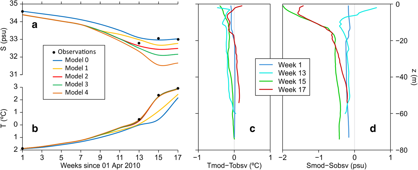
Evolution of vertically averaged water properties in Hansbukta: (a) temperature (T) and (b) salinity (S). Each model uses different configurations of subglacial discharge velocity (u _sg), whose values can be found in Table 2. Model 0 represents the evolution of the model when u _sg is zero over the entire simulation (blue line), and model 4 when u _sg is maximum (orange line). Black dots represent observations; (c) and (d) vertical distribution of modeled vs observed T and S, respectively, obtained from best-fit u _sg model (model 2). The profiles used for comparison are those of maximum depth at the end of a simulated week, and only for those weeks with an observation profile available.

Table 2.

Time series of subglacial discharge velocities (u _sg) used under different models of subglacial discharge and scenarios of submarine melting, which are described in the text and shown in Figures 5, 6, respectively

4.2. Submarine melting under three different scenarios of subglacial discharge

After calibrating the best-fit input of fresh water, varying every 2 weeks in our simulations, we also tested how the modeled SMR at the glacier front would change under different configurations of u _sg. For these simulations, we run the coupled model using a SMW-dependent CWD relation, with f-ratio = 75. Despite having already estimated the u _sg velocities which best matched the observations, we were concerned about the 2-D limitations inherent to our model. Some u _sg values could do a better job at capturing the more localized plume dynamics at the expense of unrealistic freshening of the fjord waters, while other values reduce this overfreshening but at the expense of weaker overturning that does not draw in sufficient ocean water at the fjord mouth. Consequently, we performed additional simulations with u _sg values lower (zero) and higher (double) than those resulting from the best fit, in order to obtain potential information about our 2-D model behavior, and to evaluate the sensitivity of submarine melting to subglacial discharge intensity.

Scenario 0: u _sg is assumed to be zero during the entire simulation (Table 2). This allows us to analyze how submarine melting evolves throughout the summer in the absence of turbulent buoyant plumes (though weak laminar plumes are potentially formed as submerged ice melts), thus showing the effect of ocean thermal forcing alone. It also provides information about the contribution of the boundary conditions to the change of water fjord properties in the absence of fresh water inputs.

Scenario 1: It represents the best-fit u _sg obtained in the subglacial-discharge-tuning experiment, so it can be considered as the most realistic scenario for our 2-D coupled model (see values in Table 2). Scenario1 is also used to test the influence that submarine melting exerts on glacier front dynamics (see next experiment), as well as how sensitive SMR are to spatial grid resolution (see Supplementary material, Fig. S3).

Scenario 2: In this scenario, u _sg values are the same as in scenario 1 for weeks 1–12, and then are doubled to the end of the modeling period (Table 2). This shift in u _sg represents possible sudden discharge events associated with more intense surface melting episodes not registered by our observations, and allows us to analyze the impact of the subsequent submarine ice melting on calving.

4.3. The effects of submarine melting and CWD on glacier front dynamics

In this experiment, we focus on two mechanisms controlling calving rates and front position changes during the summer: submarine melting (SMR) (Morlighem and others, Reference Morlighem2016; Seroussi and others, Reference Seroussi2017) and CWD (Cook and others, Reference Cook2014; Otero and others, Reference Otero2017). First, we analyze the contribution of submarine melting alone to calving and front position changes (Fig. 7a). We used the three different scenarios of subglacial discharge described above, while maintaining CWD equal to zero. Second, to evaluate the contribution of CWD to calving and front position, we ran the coupled model maintaining fixed the submarine melt contribution by using the best-fit subglacial discharge (i.e. scenario 1). With this configuration, we performed several runs varying CWD in two ways: (i) applying constant values of CWD = 0, 2 and 3 m; and (ii) considering surface-meltwater-dependent CWD (Eqn 10), with f-ratios = 75, 100 and 130. This experiment will allow us to determine which configuration produces the best fit between modeled and observed front position changes, and the relative importance of each mechanism in controlling calving and/or front position.

5.1. Subglacial discharge

Following previous studies, subglacial discharge intensity, Q _sg, was initially constrained by estimations of SMW (e.g. Xu and others, Reference Xu, Rignot, Menemenlis and Koppes2012; Sciascia and others, Reference Sciascia, Straneo, Cenedese and Heimbach2013), but the velocities associated with subglacial discharge, u _sg, were finally calibrated to best match observed temperature and salinity in the fjord. Due to the nearly constant vertical distribution of modeled and observed temperature and the small variations in the salinity profiles (ranging from ~32 to 34.5 psu for the entire period of simulation; Fig. 4), the profiles were vertically averaged to allow for an easy comparison of the results of our model with the observations (or interpolated data when observations were missing) every 2 weeks. Temperature and salinity in the top layer (5 m below sea level) were not considered in our calculations, since our model does not include atmospheric forcing or ice-mélange melting. Both of them could be important mechanisms in changing the physical properties of the top layers of the fjord waters, and necessary to close the heat and salt budget in our system. The point of maximum fjord depth (~200 − 350 m down-fjord from the glacial front) was selected for the comparison to collect the maximum information of the water column while avoiding the direct influence of the brackish buoyant plume. This decision was supported by the small differences observed along the rest of the fjord (see Supplementary material, Fig. S4). As mentioned earlier, estimations of minimum subglacial discharge velocities obtained from SMW were of 2 × 10⁻³ m s⁻¹. Nevertheless, fresh water discharge velocities in April (weeks 1–4) had to be reduced by half the corresponding discharge values for those dates, in order to avoid significant departures of the water properties. This could be primarily due to the limitations inherent to our 2-D model, which does not allow lateral (y-direction) mixing or redistribution of fjord and plume waters and make our fjord waters highly sensitive to fresh water inputs. Also note that we have used SMW estimations calculated for our simulating period, which involve minimum runoffs of 3 m³ s⁻¹. If there is a time lag between surface meltwater production and subglacial discharge fluxes, we are not accounting for the estimations of SMW prior to our simulations. Therefore, the time needed by SMW to reach the fjord waters could also be considered as a potential source of uncertainty and it is discussed latter in the text. Modeled temperature experienced high sensitivity to lower values of u _sg, particularly during the last weeks of the simulations. For every evaluated period, there is a threshold of u _sg from which the temperature reaches an equilibrium point that precisely matches the observations, and thereafter becomes practically insensitive to the u _sg values assessed in our study. However, the opposite pattern is exhibited by the modeled salinity: the higher the u _sg, the worse the agreement between modeled and observed salinity. An explanation for such behavior could be that, at low flow rates, the buoyancy of the plume is not strong enough to create the overturning that would draw in warmer waters from the fjord mouth, while at higher flow rates, the amount of fresh water is too large and reduces the salinity in the fjord, likely due to the lack of the third dimension in our 2-D model. Water temperature and velocities in the vicinity of the glacier front are the main variables controlling submarine melting in our system, and thus we are interested in representing them as accurately as possible. Therefore, we calibrated u _sg as that producing the best fit to the observed temperature that our model is able to reproduce, while maintaining a fair agreement with the observed salinity (see Supplementary material, Figs S2 and S5). The resulting discharge velocities that best fitted observations ranged from 10⁻³ m s⁻¹ in early April to 5 × 10⁻² m s⁻¹ in August (Table 2). Considering that the results should be evenly distributed over the missing y-direction and that the estimations of SMW reached 9 m³ s⁻¹, our 2-D best-fit model would conceptually represent a fjord up to 200 m wide for weeks with maximum fresh water inputs (weeks 15–20). This means that we are assuming a buoyant plume whose maximum lateral spreading is of 200 m, which is probably unrealistic for a 1.5 km-wide fjord. The overfreshening resulted from our fjord model point to the limitation derived from the lack of the third dimension, which in turn allow plume waters to laterally spread and mix over the rest of the fjord, not just along the 200 m that our model is able to reproduce. Our u _sg velocities for a 2-D model were considerably lower than those used by Xu and others (Reference Xu, Rignot, Menemenlis and Koppes2012) for Store glacier. This could be due to the different size of the modeled systems, since SMW fluxes in our system is over ten times lower than that estimated for Store glacier (9 vs 100 m³s⁻¹).

In Figures 5a, b, the time evolution of observed and modeled vertically averaged temperature and salinity in the fjord is shown for different configurations of fresh water inputs (Table 2) to evaluate the effects of subglacial discharge on fjord properties. For models with higher subglacial discharges (models 2–4), temperature closely resembles the observations along the summer, whereas salinity highly differs from observations, especially at the end of the summer (up to 2 psu for model 4). For those cases with u _sg being zero or lower than best-fit values (models 0 and 1), the temperature inside the fjord remains up to 2°C colder than the observations during the 15th week. This indicates that boundary forcing alone is not strong enough to change the water temperature inside the fjord. Our fjord needs a pump to generate circulation within the fjord, which would allow ocean properties to get into the system through the fjord mouth toward the glacier front, favoring submarine melting. Given the lack of surface forcing, subglacial discharge is the only source of momentum in the fjord. Therefore, the results of our experiment suggest that circulation in Hansbukta might be convectively driven by the buoyant plumes generated from subglacial discharge inputs, as has been demonstrated in other studies (Motyka and others, Reference Motyka, Hunter, Echelmeyer and Connor2003, Reference Motyka, Dryer, Amundson, Truffer and Fahnestock2013; Sciascia and others, Reference Sciascia, Straneo, Cenedese and Heimbach2013; Cowton and others, Reference Cowton, Slater, Sole, Goldberg and Nienow2015; Carroll and others, Reference Carroll2016), and that surface processes are not needed to drive the observed fjord circulation. However, for models with low u _sg (models 0 and 1), the salinity matches the observations better than those with higher u _sg (models 2–4), indicating that modeled salinity is highly sensitive to fresh water inputs. We attribute the salinity sensitivity to the limitations inherent in our 2-D model, since lateral mixing is absent.

For the best-fit configuration of u _sg (Fig. 5b, model 2, and Fig. 5c), the differences between modeled and observed temperatures were in the order of tenths of degrees Celsius or less along the entire simulation. However, modeled salinity in the fjord was more sensitive to fresh water discharge rates, which in vertical average deviated <0.3 psu from the salinity observations until mid-July, thereafter diverging from the observations by up to 0.6 psu in vertical average. Figure 5d shows the modeled–observed salinity deviations with depth for the best-fit configuration. We see that such deviations become greater (up to 2 psu at the end of week 15) in the top layer of the fjord, where the melt plume is confined. Once more, we believe that such overfreshening confined to the top layer of the fjord is mainly due to the lack of the third dimension, which does not allow lateral mixing or a more complex water redistribution. Also note that there is an increase in observed salinity in that period (Figs 4b, c), which makes highest the difference between modeled and observed salinity. Physically, the two plausible ways to increase salinity in Hansbukta would be either by evaporation at the atmosphere–ocean interface, or by intrusion of saltier waters through the fjord mouth. We attribute the observed salinity increase to sudden inputs of Atlantic water, which have been reported in previous studies (Cottier and others, Reference Cottier2010; Walczowski and Piechura, Reference Walczowski and Piechura2011), suggesting the need of stronger ocean forcing at the open boundary in terms of velocities. Our model is unable to simulate either process, since atmospheric forcing is not solved and incoming velocities at the fjord mouth are constant in time. In spite of these differences, real conditions of T and S in the fjord and their evolution throughout the summer of 2010 are fairly well represented by our model under the best-fit u _sg scenario. If we compare the time evolution of the best-fit u _sg values with that of the surface runoff estimations (SMW), we observe a time lag between the two peaks of ~4–5 weeks (Supplementary material, Fig. S5). Although our model has several simplifications (e.g. 2-D geometry, Boussinesq approximation, size of the discharge channel) and sources of uncertainties (e.g. the values chosen for all coefficients) that might affect the results quantitatively, the resulted time lag could give us an indication of the transit time of SMW through the complex englacial and subglacial hydrological system until it discharges to the fjord at the grounding line. Many studies (e.g. Xu and others, Reference Xu, Rignot, Menemenlis and Koppes2012; Sciascia and others, Reference Sciascia, Straneo, Cenedese and Heimbach2013; Mankoff and others, Reference Mankoff2016; Stevens and others, Reference Stevens2016) used SMW estimations as a proxy of subglacial discharge, assuming that all SMW discharges immediately into the fjord. However, much uncertainty remains about the hydrological processes taking place through and beneath the glacier body, as well as what proportion of SMW reaches the fjord at the grounding line vs at sea level. This finding on the time lag is neither critical to the aims of this study, nor accurately represented, since the hydrological processes are not implemented in our model. Moreover, the time resolution of our glacier model is 1 week, which constrains the precision of the time lag. Even so, it is worth to mention this time lag as a potential basis for further investigation.

5.2. Submarine melting

SMR at the submerged glacier terminus are highly dependent on both vertical (tangential to ice front) velocity and plume properties by virtue of Eqns (6–8). Plume properties are considered by the model to be the fjord properties in the column of gridcells adjacent to the ice front. Vertical velocities along the ice front wall are primarily the result of subglacial discharge fluxes, since they are the source of momentum in our model. Scenario 0, which assumes zero u _sg throughout the entire summer (Table 2), simulates the submarine melting that is produced exclusively by ocean forcing, without being amplified by subglacial discharges. Melt rates at the beginning of April were in the order of millimeters per week, evolving to 1.25 m week⁻¹ in August, with maximum reached at the grounding line (Fig. 6). Submarine melting increases up to three orders of magnitude as a result of a 5°C increase in water temperature over the summer, which highlights the importance of considering transient fjord properties when analyzing the influence of submarine melting on calving. The resulting melt rates could at a first glance seem negligible in absolute terms, as the total mass loss of the submerged front during the modeled period would be of 0.66 Mt, i.e. 1% of the total surface melting calculated for the same period (~70 Mt, according to Otero and others (Reference Otero2017)). However, when considered the cumulative melt rates per unit area over the entire simulation, oceanic forcing is almost six times more effective than atmospheric melting (8.6 vs 1.5 m, respectively). In our system, the submerged ice front area is small and insignificant when compared with the glacier surface (with a ratio of 2 : 10³). Nevertheless, ocean forcing could be expected to become important for large ice bodies embedded in the ocean, floating ice bodies with a large ocean/atmosphere ratio of surface exposure (e.g. ice shelves or icebergs).

Fig. 6.

Time evolution of submarine melt rates throughout the summer of 2010, under three different regimes of subglacial discharge velocities, u _sg. Scenario 0 assumes zero u _sg; in scenario 1 u _sg varies from 0.001 (April) to 0.05 m³ s⁻¹ (July–August); and u _sg reaches 0.1 m³ s⁻¹ (July–August) under scenario 2 (exact u _sg fluxes of each scenario are detailed in Table 2). The glacier front moves along the irregular sea bottom, thus changing the depth of submerged ice. This is represented by the white parts on the deepest zone, where there is no ice.

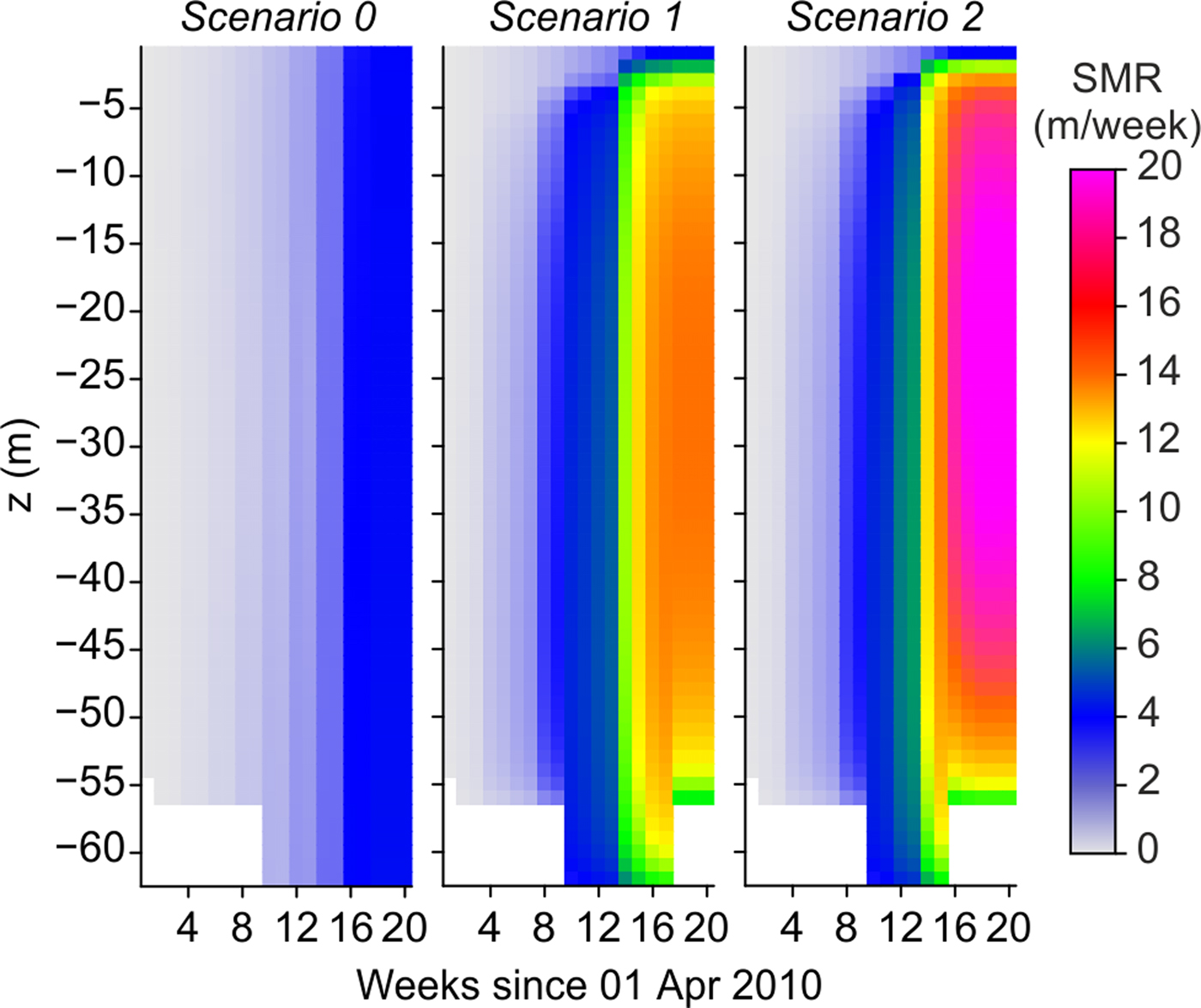
Scenario 1 represents the submarine melting obtained by using the best-fit fluxes of u _sg (see values in Table 2). In Figure 6, we observe that, under scenario 1, SMR also evolve over the summer as was described for scenario 0, but amplified by the effect of fresh water inputs, which increase tangential velocities. In April, melt rates are in the order of centimeters, and do not exceed 3 m week⁻¹ until the first week of June, then becoming comparable to observed glacier front velocities (~3 m week⁻¹). Thereafter, melt rates increase notably, reaching maximum values above 10 m week⁻¹ at 20–30 m depth and over 4 m week⁻¹ at the base of the glacier, thus starting to cause retreating of the glacier grounding point and undercutting of the ice face. Both processes grounding-point retreating and undercutting are considered to potentially affect iceberg calving and glacier front position, and will be discussed later in the text. Maximum melt rates are of ~15 m week⁻¹, reached at 20–30 m depth, from the end of July to the end of August (weeks 16–20), when water temperatures are higher and subglacial discharges are vigorous. Note that, although these values occur at the end of our simulation, they are likely to be the maximum over the year, since the mooring data in Figure S1 indicate that the fjord temperature is lower throughout the rest of the year. The cumulative melt estimations (at 20–30 m depth) during the entire period of simulation account for 108 m of submarine frontal ablation.

Under scenario 2, u _sg is doubled from week 11 (middle of June) onwards (Table 2), aiming to represent potential areas of the glacier front where the subglacial discharge could be more vigorous as the summer progresses (u _sg max = 0.1 m³ s⁻¹). Moreover, taking into account the limitations of our 2-D model, we aimed to quantify the front evolution under conditions different from those obtained as more realistic. Maximum melt rates of 20.5 m week⁻¹ are reached in August and, in general, the increase in submarine melting with respect to scenario 1 is ~25–30% (Fig. 6).

Under the two scenarios of non-zero u _sg, maximum melt rates are reached between 20 and 30 m depth, coincident with highest temperatures and maximum tangential (vertical) water velocities at the ice–ocean boundary. The SMR at these depths are within the range of 1.4–20.5 m week⁻¹, which are comparable to those obtained by other modeling studies based on larger Greenlandic systems with more intense subglacial discharge fluxes (Sciascia and others, Reference Sciascia, Straneo, Cenedese and Heimbach2013; Slater and others, Reference Slater, Nienow, Cowton, Goldberg and Sole2015). Our small glacier–fjord system reaches rates of submarine melting similar to those of much larger Greenlandic systems. The reason could be that our fjord temperatures during July–August are higher than those used for Greenlandic systems. This produces higher SMR in spite of the lower velocities of our model. Moreover, we have used higher spatial and temporal resolution, which allow us to represent smaller scale processes, as can be inferred from the sensitivity analysis (Fig. S3).

5.3. Front position changes and calving rates

Finally, we test the influence and relative importance of SMR and CWD on calving rates and front position changes. Seasonality in the dynamics of Hansbreen front is mostly influenced by the ice-mélange coverage and by basal sliding. From April to October, when ice mélange has disappeared, the glacier reaches terminus speeds of up to ~7 m week⁻¹. Our study period focuses on this time window in order to analyze the mechanisms that influence the advance and retreat of the glacier front during the period when backpressure from sea–ice is absent (Otero and others, Reference Otero2017). However, in the present study, we are not able to represent the seasonality of the glacier–fjord system, since we do not have sufficient overlapping time series of both oceanographic and glaciological data.

As a first experiment (Fig. 7a), we analyze the effects of submarine melting on glacier front position and calving, without the influence of crevasse water pressure (CWD = 0). Our results demonstrate that the addition of submarine melting amplifies the calving rates. The larger the u _sg flux, the more intense the submarine melting, and the higher the calving rates. During the 5-month modeled period, we observe that no calving events took place under scenario 0 (no fresh water inputs). Submarine melting due to ocean forcing, without the amplification derived from subglacial fresh water discharges, is insufficient to cause instabilities to the glacier front that would result in iceberg calving and consequently in front retreat. Therefore, Hansbreen front keeps advancing at speeds of 4–7 m week⁻¹, deviating from observations. For both scenarios 1 and 2, three calving events occurred from week 15 onwards, corresponding in time to maximum rates of submarine melting. They account for 17 and 34 m of cumulative frontal ablation, respectively, showing that submarine melting affects iceberg calving. However, neither scenario of submarine melting, 1 or 2, is sufficiently intense to reproduce the observed front position changes. Therefore, although submarine melting seems to be significant for Hansbreen's dynamics during late summer, having an effect on iceberg calving, it is a weak mechanism to explain front position changes when considered alone. In our study, the effects of submarine melting on calving or front position are not as remarkable as those shown by Krug and others (Reference Krug, Durand, Gagliardini and Weiss2015). Even under scenario 2, with submarine melting amplified with respect to that believed to be more representative of the real conditions (scenario 1), submarine melting alone is not enough to reproduce the front retreats observed at the end of the summer, suggesting the need of including other contributing mechanisms, such as water in crevasses.

Fig. 7.

Time evolution of Hansbreen front position for different simulations. (a) The coupled model run without the influence of crevasse water pressure (CWD = 0 m) and assuming three different scenarios of submarine melt rate (evolution of subglacial discharge intensities, u _sg, throughout the entire simulation period can be found in Table 2): zero u _sg (scenario 0), best-fit u _sg (scenario 1) and enhanced u _sg (scenario 2). (b) The coupled model run assuming submarine melting of scenario 1 (best fit) and CWD with various constant values (CWD = 0 m, green; CWD = 2 m, blue; CWD = 3 m, orange). (c) The model also runs assuming submarine melting of scenario 1, but CWD is now a function of surface melting (Eqn (10)), with f-ratios of 75 (green line), 100 (blue line) and 130 (orange line). Observations are represented as black dots.

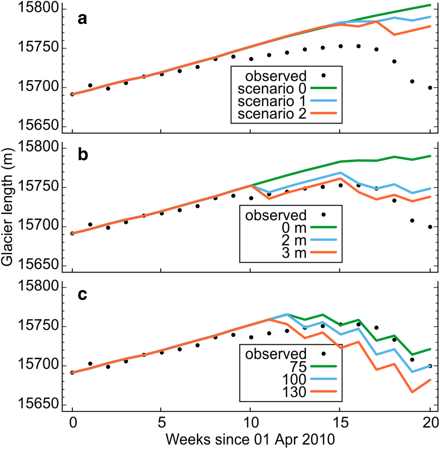
The influence of CWD on calving and front position changes, under a fixed configuration of submarine melting (given by scenario 1) is illustrated in Figures 7b, c. If CWD is considered as constant in time (Fig. 7b), the best-fit occurs when CWD = 3 m, which gives an average difference of ±12 m between observed and modeled front positions, and a cumulative frontal ablation due to calving of 73 m over the whole modeled period. Here, we note that 3 m of CWD is a lower value than that of 10 m obtained by the original uncoupled glacier model by Otero and others (Reference Otero2017), which did not consider submarine melting, thus suggesting that the inclusion of submarine melting decreases the relative importance attributed to CWD. However, since our modeled period is restricted to a single summer (2010), it is not possible to analyze the effects of a constant CWD on a multiyear simulation, as done by Otero and others (Reference Otero2017).

From a physical perspective, it seems more sensible to assume that CWDs vary in time according to surface melting runoff (SMW) derived from atmospheric forcing. As shown in Figure 7c, the model that best adjusts to front position observations is that with f = 75, which produces an average deviation lower than ±10 m, and cumulative ablation by calving of 91 m over the entire summer. In the model by Otero and others (Reference Otero2017), the best-fit ratio was f = 130. Such a value, applied to our model, results in an overestimation of frontal ablation and a retreat of the glacier front when compared with observations for the end of the modeled period (Fig. 7c). This discrepancy arises from the inclusion of the influence of submarine melting (in turn influenced by surface melting), leading to a decrease of the relative importance of runoff-dependent CWD as compared with the model by Otero and others (Reference Otero2017). The average difference between observed and modeled front positions are, in both best-fit models (with and without submarine melting), of about ±10 m, showing that the inclusion of submarine melting does not improve quantitatively the general model results in a significant way. However, the coupled model does reproduce front positions in late summer more accurately than the glacier model alone, coinciding with the period of highest submarine melting. In agreement with other studies (e.g. Morlighem and others, Reference Morlighem2016; Seroussi and others, Reference Seroussi2017), our results show that submarine melting is a relevant driver of frontal retreat and exerts a key control on calving (Vallot and others, Reference Vallot2018), but the amount of water filling the crevasses is also crucial to determine calving rates during the summer season, as indicated by Cook and others (Reference Cook2014) and Otero and others (Reference Otero2017). Therefore, our modeling suggests that submarine melting plays a significant role in the dynamics of the glacier terminus. If submarine melting is not considered in the model, larger amounts of water in surface crevasses are required to offset the terminus position so that better agreement with observations is achieved.