


Introduction
Elasticity of demand is one of the most widely used economic measures for policy analysis and understanding and forecasting market impacts of various events. Meat demand elasticity estimation in particular has been the subject of extensive past research (Gallet Reference Gallet2010; Jeon et al. Reference Jeon, Thompson, Miller, Hoang and Abler2025). Fundamental to demand elasticity estimation is having reliable and representative price and quantity data. Despite its widely recognized importance, there is a dichotomy in data used to estimate meat demand in published literature. Numerous studies have used retail meat prices reported by U.S. Department of Agriculture (USDA) that are calculated using U.S. Bureau of Labor Statistics (BLS) data and per capita disappearance derived from USDA data sources (Malla, Klein, and Presseau Reference Malla, Klein and Presseau2022; Marsh et al. Reference Marsh, Schroeder and Mintert2004; Tonsor et al. Reference Tonsor, Mintert and Schroeder2010; Tonsor and Olynk Reference Tonsor and Olynk2011). This is a “publicly available” approach to demand estimation as the data are free for users, publicly available, and easy to access. These data have been employed in meat demand estimation for decades (Gallet Reference Gallet2010; Huang Reference Huang1985).
In contrast to using USDA price and quantity data, retail point-of-sale scanner-based transaction data, “private data”, which encompass both meat prices and quantities purchased, offer an alternative data source to estimate retail meat demand. Many studies have utilized scanner data in meat demand analysis (Capps Reference Capps1989; Schulz et al. Reference Schulz, Schroeder and Xia2012; Taylor and Tonsor Reference Taylor and Tonsor2013; Zhao et al. Reference Zhao, Wang, Hu and Zheng2022). Scanner data allow for quantity-weighted retail meat price calculations, which account for increased purchase quantities at lower prices due to sales and promotions. Quantity-weighted scanner prices are typically lower than those reported by BLS which do not account for sales quantities in price reporting (Hahn et al. Reference Hahn, Perry and Southard2009; Luke et al. Reference Luke, Schroeder, Tonsor, Collins and Ufer2025; Schroeder et al. Reference Schroeder, Tonsor, Schulz, Johnson and Sommers2019). However, quantity-weighted scanner data possess limitations in that they are not publicly available, are costly to acquire, and involve considerable detail, making compiling composite retail meat prices challenging, which may hinder efficiency of their use in practice.
Of importance is how comparable demand elasticities are when estimated using the two different data sources. If there is little economic difference between the two data sources, there is limited reason to invest in more costly private data demand estimation. However, if estimated elasticities differ in economically important ways across the two data sources, careful assessment must be made of which estimates are more applicable to the research question at hand. Furthermore, product aggregation in estimation is of additional importance (Jeon et al. Reference Jeon, Hoang, Thompson and Abler2023). For example, scanner data allow for estimation of elasticities for organic and natural labeled meat products, whereas the more highly aggregated publicly available data do not. These considerations, and more, must be taken into account when determining the optimal approach to demand estimation.
The first objective is to compare U.S. meat demand elasticities estimated using the two different data sources (i.e., traditional publicly available data vs. private scanner-based data). The second objective is to use scanner data to estimate elasticities for meat products labeled organic or natural, which is not feasible using publicly available BLS price and USDA quantity data. The publicly available data are from USDA, whereas the scanner-based data are compiled by Circana (formerly Information Resources, Inc.), a market research company. We estimate and compare demand elasticities for beef, chicken, and pork using the widely applied Rotterdam demand system approach (Theil Reference Theil1980). Lensing and Purcell (Reference Lensing and Purcell2006) found smaller elasticity estimates using quantity-weighted scanner prices. However, this 2006 study included only beef cuts and encompassed data from a limited geographic area. In contrast, a recent meta-analysis found scanner data typically generate elasticities with more elastic demand than other data sources (Jeon et al. Reference Jeon, Hoang, Thompson and Abler2023). Our study estimates demand for the three main proteins consumed in the United States—beef, chicken, and pork—comparing publicly available and scanner data estimates. Our study builds on previous work using a more recent, nationwide scanner data set and estimation across major meat categories, with an additional application of estimating demands for natural and organic beef, chicken, and pork, as well.
Data
Monthly data used in this analysis span January 2009 through December 2018 for both the publicly available data and scanner data.
Description of publicly available data
The publicly available data use aggregate retail beef, chicken, and pork prices as calculated by USDA Economic Research Service (ERS). Reported ERS aggregate meat prices use retail price data collected by BLS, which do not consider purchased quantity weights for a given product within a market outlet. BLS collects retail prices for consumer products to calculate the consumer price index for all urban consumers (CPI-U), which is estimated to represent expenditure patterns of approximately 93% of the U.S. population (BLS 2023a). Each month, BLS collects approximately 94,000 retail prices. Roughly two-thirds are collected via personal visits by CPI data collectors at brick-and-mortar stores; the remaining one-third are collected through telephone calls or from visiting retailers’ websites. BLS administers an annual Consumer Expenditure Survey which is used to guide future data collection. BLS data collectors cover 75 urban areas each month and approximately 23,000 retail establishments. A multi-stage process is followed by BLS to produce a representative sample. A sample geographic area is first selected. Then a random sample of retail outlets is selected within that geographic area. Finally, BLS defines a sample of specific retail goods for which to collect prices. Typically, BLS revisits and refines the geographic sample after each decennial census. The BLS Handbook of Methods details the aforementioned procedures (BLS 2023b). While ERS conceptually outlines its price spread procedures using BLS data, it does not publish the exact method used to convert BLS meat prices to aggregate measures (Hahn Reference Hahn2004).
For quantities, the publicly available data employ per capita disappearance of beef, chicken, and pork. Disappearance is commonly considered a proxy for consumption, but it possesses notable limitations. Disappearance is derived by summing beginning stocks, production, and imports and subtracting exports and ending stocks. Production and stock data come from USDA National Agricultural Statistics Service (NASS), and trade data come from USDA Foreign Agricultural Service (FAS). In essence, disappearance represents what is “left over” from netting measured supply and utilization. Therefore, any errors in data used to calculate supply and utilization are represented in disappearance data. Additionally, disappearance data do not distinguish between domestic retail and domestic food service outlets. U.S. consumers spend a greater share of their food expenditure at food service establishments than retail outlets (USDA ERS 2022). Yet, the use of publicly available data for demand estimation solely uses retail prices in estimation because meat prices at food service establishments are not readily available.Footnote 1 Nevertheless, the use of disappearance data—as opposed to strictly retail data that excludes food service purchases—presents a limitation to this study and most others published in the U.S. meat demand literature that aim to understand solely retail demand for meat products.
Description of scanner data
The scanner-based estimates use Circana InfoScan random-weight data. InfoScan data are weekly point-of-sale scanner data aggregated to monthly to be consistent with monthly publicly available data.Footnote 2 Circana has agreements with food retailers across the U.S. to collect weekly retail product prices and quantities purchased. The collected data include purchases of random-weight, perishable products (e.g., meat), which are used in this study (Muth et al. Reference Muth, Sweitzer, Brown, Capogrossi, Karns, Levin, Okrent, Siegel and Zhen2016). InfoScan data are provided either at the individual store level or by retailer marketing area (RMA) if retailers have not granted Circana permission to release data at store levels. This study combines store-level and RMA data. Nearly 40,000 stores across the U.S. are represented in the InfoScan random-weight data. These include dollar stores, grocery stores, club stores, and mass merchandisers.Footnote 3 InfoScan data lack retail transactions from small, independent retail stores.
InfoScan data can be compared to Census Bureau data by matching North American Industry Classification System (NAICS) codes to understand its coverage. InfoScan data for 2012 covered an estimated 55% of all retail food sales in the U.S. However, coverage is not uniform across retailer types. Nearly 80% of all food sales by mass merchandisers and club stores were covered by InfoScan data in 2012. Coverage was lower for grocery and dollar stores at an estimated 50% and 19%, respectively (Muth et al. Reference Muth, Sweitzer, Brown, Capogrossi, Karns, Levin, Okrent, Siegel and Zhen2016). Given that this study is focused on retail meat purchases, small coverage of dollar stores is not a concern because these stores have limited sales of random-weight meat products (Racine et al. Reference Racine, Batada, Solomon and Story2016).
All beef, chicken, and pork product universal product codes (UPCs) were identified and extracted from the scanner data. Within each meat category, the quantity-weighted average scanner-based price (
 $ {W}_{bt}$
) for meat category b at month t was calculated as:
$ {W}_{bt}$
) for meat category b at month t was calculated as:
 $${W_{bt}} = {{\sum\nolimits_{a = 1}^z {({q_{abt}} \times {p_{abt}})} } \over {\sum\nolimits_{a = 1}^z {{q_{abt}}} }}$$
where
 $ {q}_{abt}$
and
$ {q}_{abt}$
and
 $ {p}_{abt}$
are the quantity and price, respectively, of transaction a for meat category b occurring at month t where b = beef, chicken, or pork, t = 1,…,120 (for 120 months studied), and z represents the number of observations (which differ each month).
$ {p}_{abt}$
are the quantity and price, respectively, of transaction a for meat category b occurring at month t where b = beef, chicken, or pork, t = 1,…,120 (for 120 months studied), and z represents the number of observations (which differ each month).
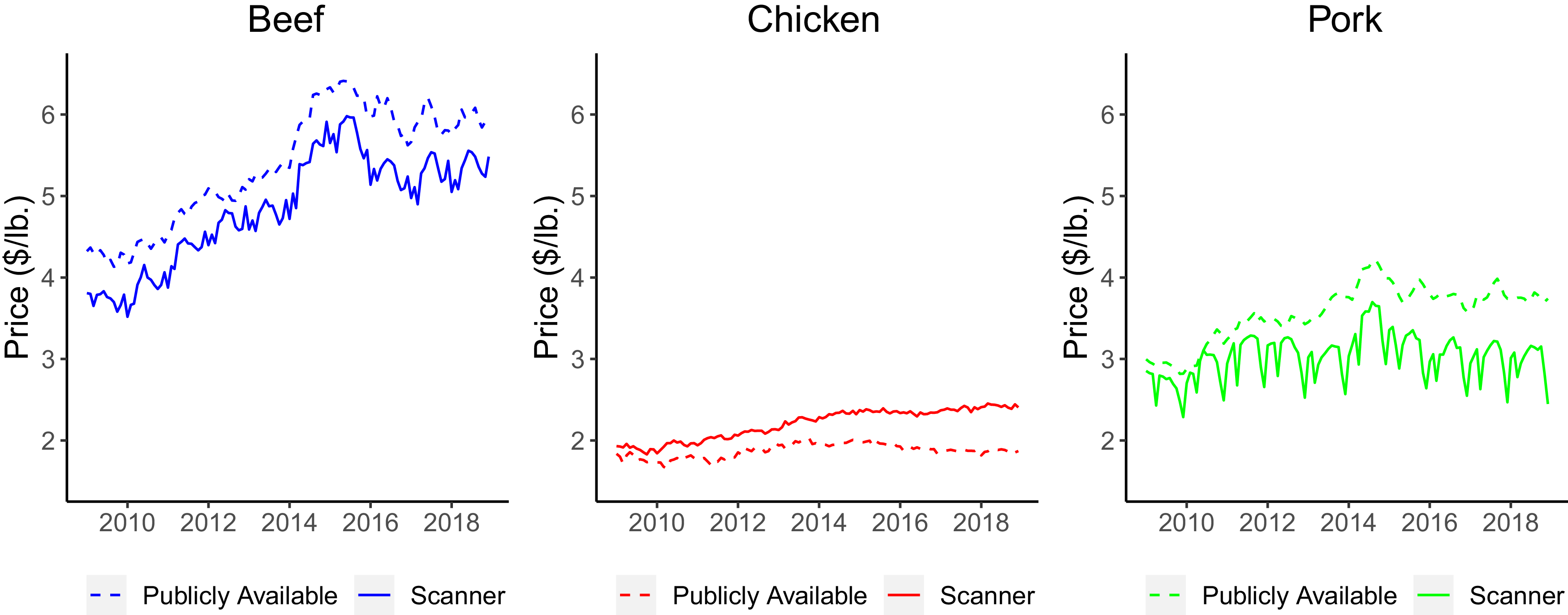
Figure 1 plots aggregate retail prices for each of the meat categories using both publicly available prices reported by ERS and quantity-weighted prices calculated from scanner data. In line with meat product-level findings by Luke et al. (Reference Luke, Schroeder, Tonsor, Collins and Ufer2025), publicly reported prices are on average greater than quantity-weighted scanner prices by 11.2% for beef and 18.1% for pork. Furthermore, scanner data illustrate greater seasonality in quantity-weighted beef and pork prices.Footnote 4 For example, ham is typically consumed around major holidays in the U.S. We find stark price dips in March or April and December each year likely due to promotions and purchases of ham for holiday festivities.Footnote 5 Conversely, beef usually sees price peaks over the summer grilling season, rather than one month in particular each year.
Aggregate retail meat prices, monthly data (January 2009–December 2018). Note: Publicly available retail prices are sourced from ERS and derived from BLS price observations. Scanner prices are quantity-weighted and calculated from Circana data.

Unlike beef and pork, the quantity-weighted price of chicken derived from scanner data is on average 14.7% higher than the retail chicken price reported by ERS. This could be in part due to the growing share of retail chicken purchased with organic or natural claims. For meat to be labeled organic, the USDA requires that “animals are raised in living conditions accommodating their natural behaviors (like the ability to graze on pasture), fed 100% organic feed and forage, and not administered antibiotics or hormones” (McEvoy Reference McEvoy2012). USDA requires meat labeled natural to be a product “containing no artificial ingredient or added color and is only minimally processed. Minimal processing means that the product was processed in a manner that does not fundamentally alter the product. The label must include a statement explaining the meaning of the term natural (such as ‘no artificial ingredients; minimally processed’)” (USDA Food Safety and Inspection Service 2015). Employing these measures and facilitating the labeling process increases the cost of production for organic and natural meat. As such, meat products featuring these claims are sold at a premium in the retail setting.
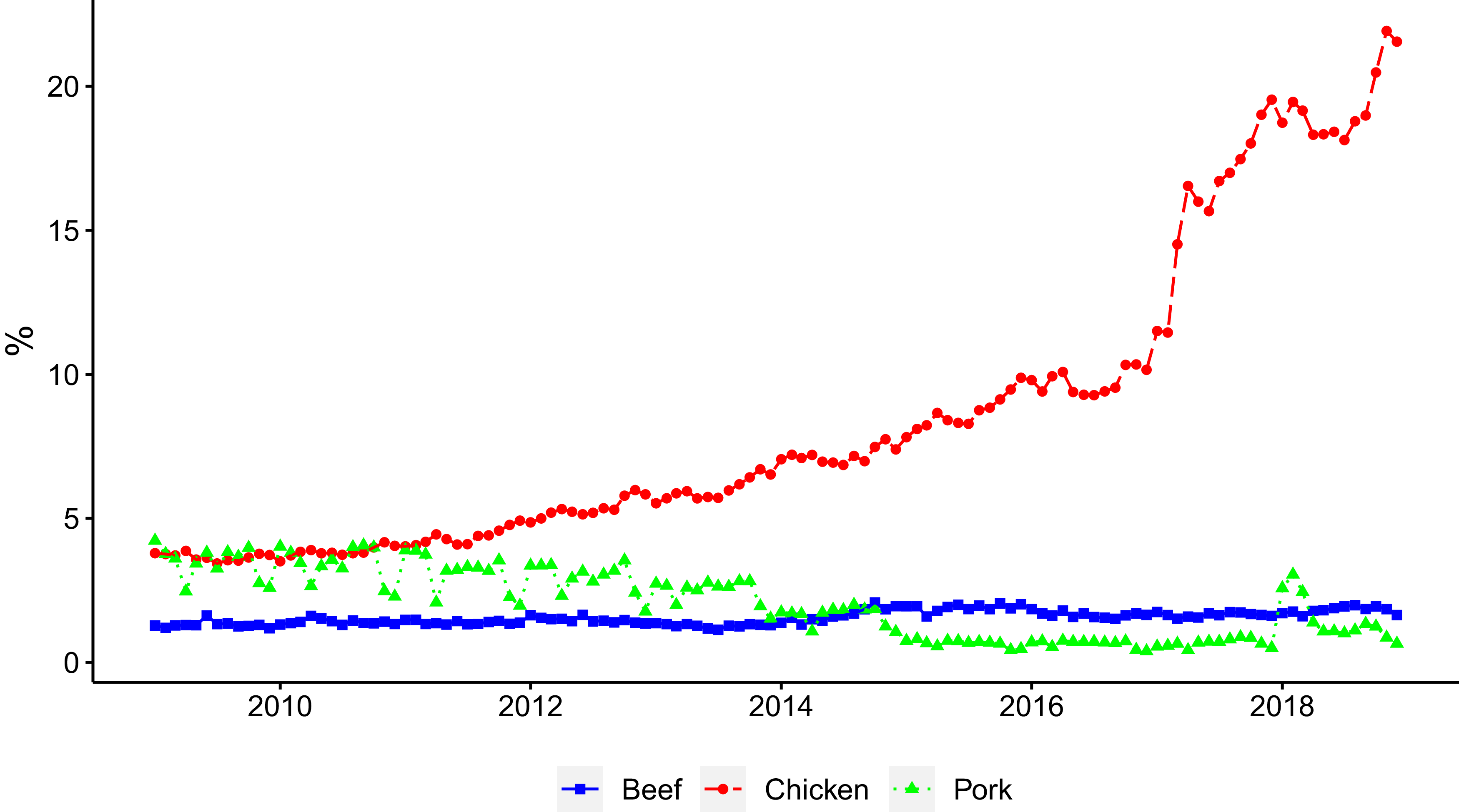
In Figure 2, we plot the share of purchased quantities of beef, chicken, and pork in the scanner data set that carry an organic or natural label. Figure 2 reveals that the shares of organic or natural beef remains steady and pork declines over the span of our data, both being less than 5%.Footnote 6 Conversely, the share of organic and natural chicken purchased increases substantially. Circana data reveal that in 2009 an average of 3.7% of all retail chicken purchased was organic or natural and by 2018 that number had grown to 19.4%.Footnote 7 Because BLS data series do not differentiate between chicken with and without organic or natural claims, aggregate price estimates derived from BLS data have embedded in them evolving demand for organic or natural chicken products. Additionally, given the limited scope of the number of BLS retail chicken price series available to calculate an aggregate retail chicken price, the weighting process used by ERS may not be representative of consumer purchase shares.
Share of beef, chicken, and pork quantities purchased with organic or natural claims, monthly scanner data (January 2009–December 2018). Note: Underlying scanner data are sourced from Circana. Plotted shares are calculated by the authors.

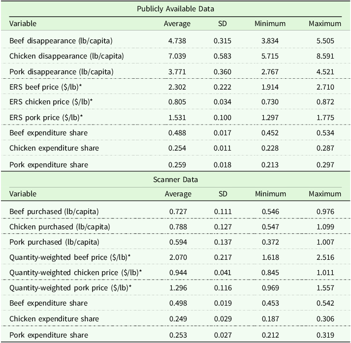
Table 1 summarizes statistics for both the publicly available and scanner-based data over the 120 monthly observations in our data set. Per capita disappearance is considerably greater for each of the meat categories as compared to per capita quantity purchased represented in the scanner data set. Scanner data purchase quantities are, on average, 15.3%, 11.2%, and 15.8% of disappearance quantities for beef, chicken, and pork, respectively.Footnote 8 For both data sets, chicken has the highest per capita disappearance/purchased quantities followed by beef and then pork.
Summary statistics of monthly data used to estimate Rotterdam demand models (January 2009–December 2018)

Note: *denotes inflation-adjusted dollars (deflated by Consumer Price Index, 1982-1984 = 100).
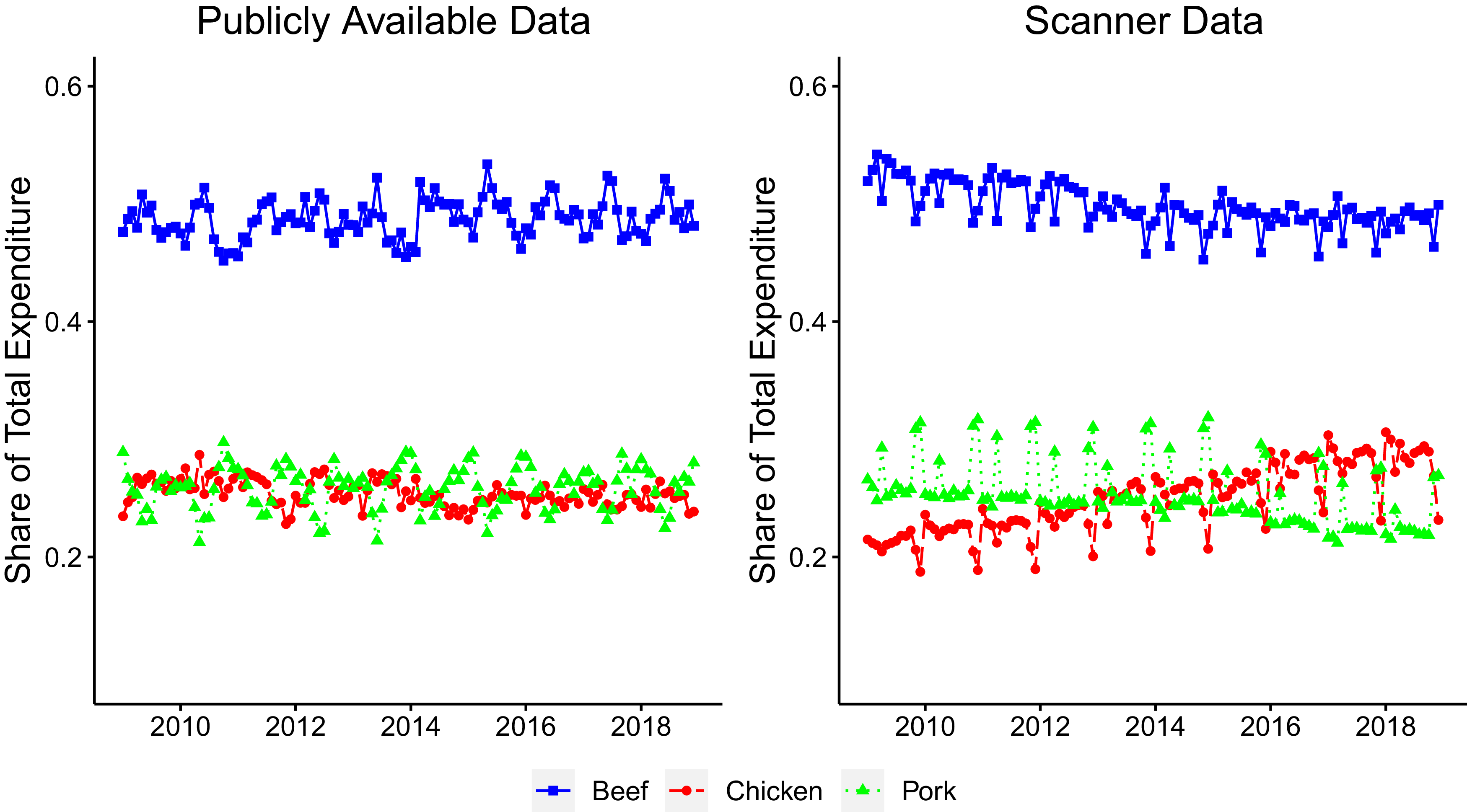
Beef, chicken, and pork expenditure shares are presented in Table 1 and Figure 3. Average expenditure shares for beef are greater than for the other two meat categories using both public and private data sources. Figure 3 reinforces average findings and shows that, using publicly available data, beef expenditure share exceeds chicken and pork, and expenditure shares for chicken and pork are similar. The scanner data reveals a greater expenditure share for pork than chicken in the beginning of the period, but the chicken expenditure share increases while beef and pork shares decrease over time. As such, chicken expenditure share exceeds that for pork in recent years. Figure 3 further illustrates seasonality in pork share in scanner data is more pronounced than publicly available data sources indicate.
Share of total expenditure by meat category using publicly available data and scanner data, monthly data (January 2009–December 2018). Note: Underlying publicly available data are sourced from USDA, and scanner data are sourced from Circana. Plotted shares are calculated by the authors.
Methods
While the data sources differ, our elasticity estimation procedures are identical between the two data sets.Footnote 9 Demand analyses frequently use the Rotterdam demand model (Brester and Schroeder Reference Brester and Schroeder1995; Capps and Love Reference Capps and Love2002; Nayga and Capps Reference Nayga and Capps1994; Tonsor and Olynk Reference Tonsor and Olynk2011) as it provides a flexible functional form, enabling theoretical demand restrictions to be imposed.Footnote 10 The base Rotterdam model is adapted to include seasonal parameters. Additionally, a meat separability assumption is made to complete this analysis following published literature (Coffey et al. Reference Coffey, Schroeder and Marsh2011; Piggott and Marsh Reference Piggott and Marsh2004; Tonsor and Marsh Reference Tonsor and Marsh2007). This implies that changes in meat demands produce a net zero effect on total meat expenditure, which aids in understanding the relationships that exist among beef, chicken, and pork. It also assumes no spill-over effects in non-meat foods or non-foods.
For n goods, the budget share equations underlying the Rotterdam model are:
 $$ {w}_{i}\Delta {\rm l}{\rm n}\left({q}_{i}\right)={\beta }_{i}\Delta \mathrm{}{\rm l}{\rm n}\left({\bar{q}}\right)+\sum\limits _{j=1}^{n}{c}_{ij}\Delta {\rm ln}\left({p}_{j}\right)+\sum \limits_{k=1}^{3}{d}_{ik}{D}_{k}+{u}_{i}$$
where
 $ {w}_{i}$
is the budget share of the ith good (i = 1,…,n),
$ {w}_{i}$
is the budget share of the ith good (i = 1,…,n),
 $ \Delta $
is the across-period first difference operator, and
$ \Delta $
is the across-period first difference operator, and
 $ {q}_{i}$
is the quantity of good i. The Divisia volume index (DVI) is given by
$ {q}_{i}$
is the quantity of good i. The Divisia volume index (DVI) is given by
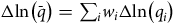 $ \Delta \mathrm{}{\rm l}{\rm n}\left(\bar{q}\right)={\sum }_{i}{w}_{i}\Delta {\rm l}{\rm n}\left({q}_{i}\right)$
, and
$ \Delta \mathrm{}{\rm l}{\rm n}\left(\bar{q}\right)={\sum }_{i}{w}_{i}\Delta {\rm l}{\rm n}\left({q}_{i}\right)$
, and
 $ {p}_{j}$
is the price of good j. Quarterly binary variables are denoted by
$ {p}_{j}$
is the price of good j. Quarterly binary variables are denoted by
 $ {D}_{k}$
, and k = 1, 2, and 3, for the first, second, and third quarters of the year, respectively. The error term is
$ {D}_{k}$
, and k = 1, 2, and 3, for the first, second, and third quarters of the year, respectively. The error term is
 $ {u}_{i}$
. Finally,
$ {u}_{i}$
. Finally,
 $ {\beta }_{i}$
,
$ {\beta }_{i}$
,
 $ {c}_{ij}$
, and
$ {c}_{ij}$
, and
 $ {d}_{ik}$
are all parameters to be estimated.
$ {d}_{ik}$
are all parameters to be estimated.
Theoretical restrictions of adding up are imposed by:
 $$ \sum\limits _{i=1}^{n}{\beta }_{i}=1,\sum\limits _{i=1}^{n}{c}_{ij}=0,{\rm and}\sum\limits _{k=1}^{3}{d}_{ik}=0.$$
Homogeneity and symmetry restrictions are imposed by:
 $$ \sum\limits _{j=1}^{n}{c}_{ij}=0\;{\rm and}\mathrm{}\;\mathrm{}{c}_{ij}={c}_{ji}\forall i\ne j.$$
When estimating demand systems, one equation must be dropped to avoid singularity of the underlying variance-covariance matrix. However, given imposed restrictions, the parameters of the omitted equation can be recovered.
Considering potential endogeneity concerns among quantities and/or prices in meat demand estimation, Hausman specification tests are conducted following Thurman (Reference Thurman1986). The model is estimated first assuming price and expenditure are predetermined using the iterative seemingly unrelated regression (ITSUR) technique. Second, assuming prices and expenditures are endogenous, the iterative three-stage least squares (IT3SLS) technique is used. Following Eales and Unnevehr (Reference Eales and Unnevehr1993), Kinnucan et al. (Reference Kinnucan, Xiao, Hsia and Jackson1997), and Tonsor and Olynk (Reference Tonsor and Olynk2011), instruments used in estimation include corn and soybean prices received by producers, an energy price index, an animal slaughter and processing price index, the bank prime loan rate, meat processed from animal carcasses, quarterly binary variables, per capita meat expenditure, and lagged prices.Footnote 11 The null hypothesis of exogeneity is rejected; the presented results are produced from IT3SLS estimation.
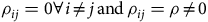
Given the time series nature of the data being used and following Piggott and Marsh (Reference Piggott and Marsh2004), Tonsor and Marsh (Reference Tonsor and Marsh2007), and Tonsor and Olynk (Reference Tonsor and Olynk2011), three different Berndt and Savin (Reference Berndt and Savin1975) autocorrelation corrections are evaluated. These three corrections include: (i) null matrix: a correction matrix restricting all elements to zero (i.e., no autocorrelation correction,
 $ {\rho }_{ij}=0\forall ij$
), (ii) diagonal matrix with one common term: a correction matrix with all off-diagonal elements restricted to zero and all diagonal elements restricted to one common term (
$ {\rho }_{ij}=0\forall ij$
), (ii) diagonal matrix with one common term: a correction matrix with all off-diagonal elements restricted to zero and all diagonal elements restricted to one common term (
 $ {\rho }_{ij}=0\forall i\ne j\,{\rm and}\,{\rho }_{ij}=\rho \ne 0$
 $ \forall i=j$
), and (iii) diagonal matrix with differing terms: a correction matrix with all off-diagonal elements restricted to zero and all diagonal elements differing individually (
$ \forall i=j$
), and (iii) diagonal matrix with differing terms: a correction matrix with all off-diagonal elements restricted to zero and all diagonal elements differing individually (
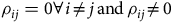 $ {\rho }_{ij}=0\forall i\ne j\,{\rm a}{\rm n}{\rm d}\,{\rho }_{ij}\ne 0$
 $ \forall i=j$
). Traditional likelihood ratio tests used to compare alternate model specifications rely on asymptotic assumptions, so adjusted likelihood ratio tests are used instead given the small sample sizes (Bewley Reference Bewley1986). For both the publicly available data and scanner-based data, the null correction matrix is rejected in favor of the diagonal matrix with one common term, but we fail to reject the diagonal matrix with one common term in favor of the diagonal matrix with differing terms. Consequently, results reflect the use of the diagonal autocorrelation correction matrix with one common term.
$ \forall i=j$
). Traditional likelihood ratio tests used to compare alternate model specifications rely on asymptotic assumptions, so adjusted likelihood ratio tests are used instead given the small sample sizes (Bewley Reference Bewley1986). For both the publicly available data and scanner-based data, the null correction matrix is rejected in favor of the diagonal matrix with one common term, but we fail to reject the diagonal matrix with one common term in favor of the diagonal matrix with differing terms. Consequently, results reflect the use of the diagonal autocorrelation correction matrix with one common term.
Using raw demand system coefficients estimated in equation (2), post-estimation calculations are needed to determine Hicksian (compensated) price elasticities and expenditure elasticities. The compensated price elasticity for good i with respect to good j is
 $$ {\epsilon}_{ij}={{{c}_{ij}}\over{{w}_{i}}}.$$
The expenditure elasticity for good i is calculated by
 $$ {e}_{i}={{{\beta }_{i}}\over{{W}_{i}}}.$$
Elasticities are calculated at the means of the explanatory variables. To determine statistical significance of the elasticity point estimates, a Krinsky and Robb (Reference Krinsky and Robb1986) simulation-based evaluation of elasticities is conducted. One thousand values of each estimated elasticity are generated using random draws from a multivariate normal distribution based on the estimated coefficients and variance terms of the model. Confidence intervals are then determined. For an elasticity point estimate to be statistically significant at the 10%, 5%, and 1% levels, the null hypothesis (i.e., Ho = 0, Ho = 1, or Ho = −1) should not fall within the corresponding 90%, 95%, and 99% confidence intervals, respectively. Statistical significance of differences between elasticities is determined following the complete combinatorial method outlined in Poe, Giraud, and Loomis (Reference Poe, Giraud and Loomis2005).
Previous work has used out-of-sample testing to compare elasticity estimates (Kastens and Brester Reference Kastens and Brester1996). Similarly, we compare publicly available and scanner data elasticities by following the previously outlined demand estimation procedures using only the observations spanning January 2009 through December 2016. New elasticity measures are calculated using coefficients from the new estimations. These new elasticities, as well as observed prices for January 2017 through December 2018, are used to predict monthly quantities for the out-of-sample period. Once predicted quantities are determined, the root mean squared percentage error (RMSPE) is calculated for good i using the following:
 $$ {RMSPE}_{id}=100\times \sqrt{{{\sum }_{m=Jan\,2017}^{Dec\,2018}{({\rm l}{\rm n}{A}_{idm}-{\rm l}{\rm n}{P}_{idm})}^{2}}\over{\mathrm{T}}}$$
where i represents beef, chicken, and pork, d represents publicly available and scanner data sets, and m = 1,…,24 (for the 24 months spanning January 2017 through December 2018). The actual, realized quantity is represented by
 $ {A}_{idm}$
, and the predicted quantity is represented by
$ {A}_{idm}$
, and the predicted quantity is represented by
 $ {P}_{idm}$
. T is equal to 24 for the 24 months included in the out-of-sample prediction window.
$ {P}_{idm}$
. T is equal to 24 for the 24 months included in the out-of-sample prediction window.
Results
Coefficients from the Rotterdam model estimations conducted using SAS 9.4 software are summarized in Table 2. Statistically significant seasonality is present across quarters and meat categories for the public data estimates but not for scanner data results. Seasonal variation in featuring activity, as documented by USDA’s weekly national retail reports for beef, chicken, and pork (USDA AMS 2023), is controlled for in the scanner data because prices are quantity-weighted. That is, seasonal quantity differences evident in scanner data are embedded in the quantity-weighted scanner data prices unlike in the publicly available data. The primary aspect of featuring in the public data is via the seasonal intercept shifters.
Coefficient estimates of Rotterdam model using publicly available data and scanner data, monthly data (January 2009–December 2018)
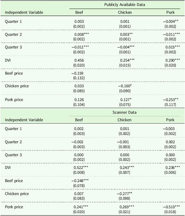
Note: Standard errors are in parentheses. *, **, and *** denote statistical significance at the 10%, 5%, and 1% level, respectively. R 2 statistics are 91.4%, 84.1%, and 74.4% for beef, chicken, and pork, respectively, using publicly available data. R 2 statistics are 98.0%, 94.1%, and 96.8% for beef, chicken, and pork, respectively, using scanner data. DVI is the Divisia volume index.
Using estimated coefficients from Table 2, we calculate compensated price and expenditure elasticities reported in Table 3. Compensated own-price elasticities for all meat categories using both data sources are negative, and all but the publicly available beef own-price elasticity are statistically different from zero. These findings are in line with expectations. That is, for example, using the publicly available data suggests that a 1% increase in the price of chicken leads to a 0.630% decrease in the quantity of chicken demanded. Thus, the own-price elasticity for chicken is inelastic. Similar findings exist for both beef and pork with own-price elasticities of −0.327 and −0.978, respectively. Our own-price elasticity estimates for beef and pork are in line with previous studies that utilized publicly available data (Tonsor et al. Reference Tonsor, Mintert and Schroeder2010; Tonsor and Olynk Reference Tonsor and Olynk2011). However, our chicken own-price elasticity is more elastic than the poultry own-price elasticities reported in these studies. This could be attributed to the inclusion of turkey in the poultry category in these older studies or to the more recent timespan of our data. Recent elasticity estimates for beef (−0.383), poultry (−0.606), and pork (−0.813) are similar to our estimates using publicly available data (Malla, Klein, and Presseau Reference Malla, Klein and Presseau2022). All cross-price elasticities using the publicly available data are positive, suggesting substitutability between each of the meat categories, but the elasticities lack statistical significance at standard levels.
Estimated compensated price elasticities and expenditure elasticities of Rotterdam models, monthly data (January 2009–December 2018)
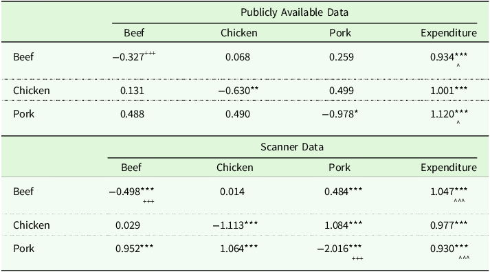
Note: Elasticities are calculated at the mean values of the explanatory variables. The columns and rows of the table correspond to price and quantity changes, respectively. p-values are calculated using a Krinsky-Robb (Reference Krinsky and Robb1986) bootstrapping approach. *, **, and *** denote elasticities statistically different from zero at the 10%, 5%, and 1% significance level, respectively. +, ++, and +++ denote own-price elasticities statistically different from negative one at the 10%, 5%, and 1% significance level, respectively. ^, ^^, and ^^^ denote expenditure elasticities statistically different from one at the 10%, 5%, and 1% significance level, respectively.
Similar to the publicly available data, own-price elasticities from the scanner data indicate consumers are least price sensitive regarding beef and most price sensitive regarding pork. Unlike the publicly available data, the scanner data own-price elasticities for chicken and pork are elastic. That is, a 1% increase in the price of chicken, for example, implies a 1.113% decrease in the quantity demanded. Each of the scanner-based own-price elasticities is greater in magnitude than those estimated with publicly available data, which is in line with Jeon et al. (Reference Jeon, Hoang, Thompson and Abler2023). In contrast to the publicly available data, all but two of the cross-price elasticities are statistically significant. Cross-price elasticities estimated from the scanner data suggest substitutability within the demand system and are typically larger in magnitude than those estimated from the publicly available data. This suggests a higher degree of substitutability across meats by consumers when estimating demand using scanner data as compared to publicly available data.
Each of the estimated expenditure elasticities is statistically different from zero, but the two data sources provide disparate conclusions regarding responsiveness of each meat category to expenditure changes. Publicly available data estimates suggest that beef is a necessity good while chicken and pork are luxury goods. On the contrary, scanner data estimates indicate that beef is a luxury good while chicken and pork are both necessity goods.
We used simulated Krinsky and Robb (Reference Krinsky and Robb1986) elasticity vectors and the Poe, Giraud, and Loomis (Reference Poe, Giraud and Loomis2005) complete combinatorial approach to test statistical differences in elasticity estimates across data sources. Many of the elasticities estimated using publicly available data are statistically different from corresponding scanner data elasticities. In particular, pork own-price elasticity, beef cross price with pork, chicken cross price with pork, and pork with respect to chicken cross-price elasticities are statistically different across the two data sources. Furthermore, using publicly available data, only beef and pork own-price elasticities are statistically different from one another. Using scanner data, each of the own-price elasticities are statistically different from one another. Of the cross-price elasticities calculated from publicly available data, none are statistically different from one another. However, using scanner data, beef cross-price elasticities with respect to chicken and pork are statistically different, chicken cross-price elasticities with respect to beef and pork are statistically different, and pork cross-price elasticities with respect to beef and chicken are statistically different. In essence, scanner data provide more statistically different elasticity estimates than publicly available data, which uncovers important insights into relationships that exist among meat categories.
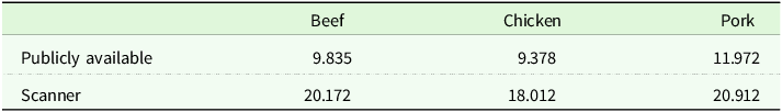
Table 4 summarizes the RMSPE for out-of-sample quantity predictions using both data sources. For beef, chicken, and pork the RMSPE for publicly available data is less than that calculated using the scanner data. These results indicate a greater degree of accuracy in out-of-sample predictability in meat demand estimation using publicly available data as compared to scanner data across the three proteins, with beef exhibiting the largest difference between publicly available and scanner RMSPEs. That said, scanner data still possess advantages over publicly available data in some demand estimation applications. As discussed in the next section, scanner data allow for a greater level of aggregation. Hence, estimating demand for natural or organic products is possible with these data. The research question being explored should ultimately dictate which data set is chosen for analysis, considering any limitations that may be present.
Root mean squared percentage error (RMSPE) for out-of-sample quantity predictions (January 2017–December 2018)

Note: Sample data used in estimating coefficients for calculating out-of-sample quantity predictions spanned January 2009 to December 2016.
Discussion and further application
Meat quantity-weighted scanner prices account for greater quantities purchased at lower prices. As such, scanner-based prices were expected to be lower than retail meat prices reported by ERS that are calculated using BLS data. Beef and pork prices derived from scanner data are indeed lower than those reported by ERS, but the opposite is true for chicken. Own-price elasticities estimated using scanner data are greater in magnitude, indicating consumers are more price sensitive than elasticities estimated using publicly available data suggest. Results are consistent with Jeon et al. (Reference Jeon, Hoang, Thompson and Abler2023). Previous work ranking consumer food preferences and purchasing determinants ranks price among the highest product purchasing factors (Ardebili and Rickertsen Reference Ardebili and Rickertsen2023; Lister et al. Reference Lister, Tonsor, Brix, Schroeder and Yang2017; Lusk and Briggeman Reference Lusk and Briggeman2009; Osman et al. Reference Osman, Schroeder, Lancaster and White2024; ; Tonsor Reference Tonsor2023). Our results regarding greater price sensitivity reinforce the importance of price when consumers make meat protein purchase decisions.
Jeon et al. (Reference Jeon, Hoang, Thompson and Abler2023) further proposes “correction procedures” to reconcile differences between elasticities that are and are not derived from retail scanner data. Specifically, a correction of −0.219 is suggested to align non-scanner-based own-price elasticities to retail scanner-based own-price elasticities. Though this adjustment factor likely would vary across food products having varied elasticities, we use it here as reported in Jeon et al. (Reference Jeon, Hoang, Thompson and Abler2023) as a single fixed value across products for exemplary purposes. In our study, the publicly available own-price elasticity for beef (−0.327) would be updated to −0.546 using the proposed correction factor, slightly less inelastic than −0.498, the beef own-price elasticity estimated using the retail scanner data. For chicken, the publicly available own-price elasticity (−0.630) would be −0.849 after calibration. This indicates the own-price elasticity for chicken would remain inelastic, whereas the scanner data derived elasticity in our study (−1.113) is elastic. Finally, the pork own-price elasticity estimated from the publicly available data (−0.978) would be calibrated to −1.197, less elastic than the −2.016 elasticity we derived from scanner data demand estimation.
Elasticity calculations are a function of both price and quantity changes. Monthly meat disappearance quantities in publicly available data are much greater than those observed in scanner data—sometimes by a factor of ten or more. To reiterate, the two data sources do not measure the same value of interest. Publicly available data use calculated disappearance to measure what is “left over” when accounting for changes in monthly stocks, trade, and production. Thus, it captures the domestic retail market, the domestic food service market, and any errors in calculation or reporting of stocks, trade, and production. Scanner data quantity captures only a subset of the domestic retail market. While it is a sizeable share of the market (approximately 55%), it does not capture any meat flowing through food service establishments.
Given these data discrepancies and limitations, it is of no surprise that differences in results exist. Largely, if research questions demand insights at the retail level, elasticity estimates derived from scanner data are most applicable. For example, Van Loo et al. (Reference Van Loo, Caputo and Lusk2020) finds 36% of respondents of a U.S. nationwide survey would support a 10% tax on beef to reduce beef consumption for environmental and animal welfare objectives. Assuming this tax is applied solely to retail purchases, our scanner data elasticities indicate that the 10% tax would result in an estimated decrease in beef quantity demanded of 4.98%, compared to a decrease of only 3.27% using the publicly available data. While both indicate inelastic responses by consumers, the difference of nearly 2% in quantity of beef demanded is sizeable when considering current market fundamentals in the U.S. beef sector today. If, however, the proposed tax would apply to all beef purchases (retail and foodservice alike), the publicly available data elasticity estimate may be more indicative of the potential market impacts.
Going forward, gaining access to a greater amount of scanner data as well as teasing out domestic retail versus food service quantities in the publicly available disappearance series would be of value to make more direct comparisons of demand estimation across the two data sources. However, disaggregated disappearance data are currently unavailable for a number of reasons, including limited tracking of transactions within the U.S. food service industry.
Potential causes of greater price sensitivity in meat demand could also stem from the unexpected result that scanner-based quantity-weighted chicken prices are greater than those reported by ERS. This could have a substantial impact given it is the meat category with the greatest amount of disappearance (about half the meat consumed in the U.S. is poultry) and quantity purchased in the respective data sets. This finding may follow from the increasing share of chicken purchased with an organic or natural claim.
To explore this finding further, we re-estimated the demand system using scanner data and disaggregate organic/natural purchases from nonorganic/natural meat purchases, which we will refer to as “no claim”.Footnote 12 Summary statistics of the data used, outlined in Table 5, show that meat products labeled organic or natural carry a premium as compared to their counterparts without such labels. The calculated average premium for organic/natural using scanner data is 60% for beef, 85% for chicken, and 32% for pork.
Summary statistics of monthly scanner data used to estimate Rotterdam model with organic/natural purchases disaggregated (January 2009–December 2018)
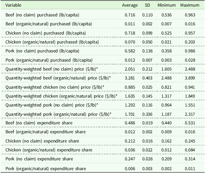
Note: *denotes inflation-adjusted dollars (deflated by Consumer Price Index, 1982–1984 = 100).
For brevity, coefficient estimates are available in Table A1 in the Appendix. Elasticity estimates, calculated using the estimated coefficients, are summarized in Table 6. Consumers are more price sensitive when purchasing organic/natural meat products as compared to those with no claims. That is, for each meat category the organic/natural own-price elasticity is larger in magnitude than the no claim own-price elasticity. This is most evident regarding beef, whose organic/natural own-price elasticity (−1.389) is nearly triple its no claim own-price elasticity (−0.466). Further, all but one own-price elasticities is larger in magnitude in the disaggregated system as compared to the aggregated approach (whose results are summarized in the lower half of Table 3). This is in line with economic theory as more substitutes are available when goods are further disaggregated. It follows that demand for disaggregated goods would be more price sensitive as the consumer choice set expands, which is consistent with the results of our study.
Estimated compensated price elasticities of Rotterdam models, monthly scanner data (January 2009–December 2018)
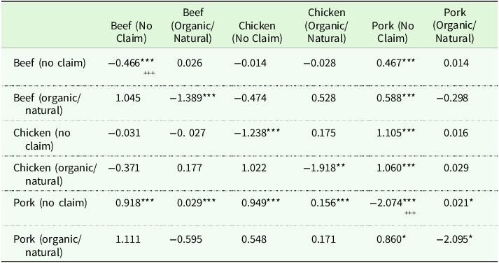
Note: Elasticities are calculated at the mean values of the explanatory variables. The columns and rows of the table correspond to price and quantity changes, respectively. p-values are calculated using a Krinsky-Robb (Reference Krinsky and Robb1986) bootstrapping approach. *, **, and *** denote own- and cross-price elasticities statistically different from zero at the 10%, 5%, and 1% significance level, respectively. +, ++, and +++ denote own-price elasticities statistically different from negative one at the 10%, 5%, and 1% significance level, respectively.
Although not all statistically significant, we mostly find substitutability among meats, especially between no claim and organic/natural specifications within a particular meat category. For example, a 1% increase in the price of no claim pork leads to a 0.860% increase in quantity demanded of organic/natural pork. Conversely, a 1% increase in the price of organic/natural pork results in only a 0.021% increase in quantity demanded of no claim pork. This trend in cross-price elasticity magnitudes within meat categories follows for both beef and chicken. Perhaps, consumers who regularly consume meat products with an organic or natural claim are less likely to substitute products without an organic or natural claim than consumers who typically purchase products without an organic or natural claim are to substitute organic or natural products. Future research using household transaction data could tease out this finding further and is encouraged given industry-wide trends in product differentiation.
Ultimately, both data source and aggregation level are pertinent in demand estimation. Further disaggregation of scanner data reveals demand differences for premium specialty meat products. Yet, this showcases just one facet of the information that underlies scanner data. Going forward, numerous extensions of this study could be pursued to better understand intricacies of U.S. meat demand; we hope our analysis motivates corresponding additional research.
Conclusion
Quantity-weighted scanner-based beef and pork prices are lower than those reported by USDA, whereas quantity-weighted chicken prices are higher. Own-price elasticities for beef, chicken, and pork are larger in magnitude using scanner data as compared to traditionally relied upon publicly available data. Meat consumers may be more price sensitive than indicated by elasticity estimates from publicly available data sources.
Data limitations present an issue in comparing estimated elasticities from the two data sources. Publicly available data measures disappearance quantities, which include both domestic retail and domestic food service, but scanner data considers only a share of the domestic retail market. Thus, this study cannot explicitly be an “apples-to-apples” comparison. Existing differences in data measurements almost assuredly impact results and are difficult to reconcile without richer data. Unfortunately, little data are available measuring the quantity (and accompanying price) of beef, chicken, and pork sold through food service establishments.
Nevertheless, we showcase the rich insights that can be garnered via the use of scanner data in demand estimation. Specifically, by disaggregating beef, chicken, and pork into organic/natural labeled products, we determined that consumers are more price sensitive to these products as compared to no-claim counterparts. Further, a greater degree of substitutability of organic/natural products for no-claim products is present than no claim products for organic/natural products. Thus, consumers who typically purchase organic/natural meat are committed to purchasing products with such labels.
Going forward, practitioners should be cognizant of differences between elasticity estimates calculated from different data sources. Potential shortcomings exist for use of both publicly available data and scanner data in meat demand estimation. However, scanner data can provide a more accurate measure of consumer retail purchases relative to publicly available data and therefore may better reflect variation in grocery store expenditures. As such, we encourage consideration of scanner data insights in retail demand elasticity estimation when possible. Ultimately, further research is needed to fully characterize the contribution that scanner data could make in meat demand research.
Supplementary material
The supplementary material for this article can be found at https://doi.org/10.1017/age.2025.10020
Data availability statement
The publicly available data that support the findings of this study are available from the corresponding author, Jaime R. Luke, upon reasonable request. The scanner-based data that support the findings of this study are available from Circana. Restrictions apply to the availability of these data, which were used under license for this study.
Acknowledgments
This study was supported in part by the U.S. Department of Agriculture, Economic Research Service. The findings and conclusions in this publication are those of the authors and should not be construed to represent any official USDA or U.S. government determination or policy.
Funding statement
This research received no specific grant from any funding agency, commercial, or not-for-profit sectors.
Competing interests
The authors declare none.


 Open access