

1. Introduction
Historically, crude oil has been an input to agricultural production; therefore, the direction of influence tended to go from crude oil prices to agricultural prices, but not the other way around. With an increase of corn utilized for ethanol and distiller's dried grains with solubles production—from 5% to nearly 40%—the relationship between agricultural and energy commodity prices has adapted to new market conditions (Abbott, Hurt, and Tyner, Reference Abbott, Hurt and Tyner2008). A number of authors have suggested that in this new era, energy prices play a more important role in agricultural commodity prices (Gohin and Chantret, Reference Gohin and Chantret2010; Tyner, Reference Tyner2010; Zhang et al., Reference Zhang, Lohr, Escalante and Wetzstein2010). Yet, the literature still has not identified a clear mechanism of integration between oil and agricultural markets (Algieri, Reference Algieri2014; Du and Hayes, Reference Du and Hayes2009; Haixa and Shiping, Reference Haixa and Shiping2013; Nazlioglu, Reference Nazlioglu2011; Nazlioglu and Soytas, Reference Nazlioglu and Soytas2012; Reboredo, Reference Reboredo2012; Thompson, Meyer, and Westhoff, Reference Thompson, Meyer and Westhoff2009; Whistance and Thompson, Reference Whistance and Thompson2010).
Regardless of the debated relationship between energy and agricultural markets, one would expect a connection between the commodities to manifest itself at least through volatility spillovers. In other words, we expect more informational spillovers between corn and crude oil prices because of more tightly integrated markets for corn, crude oil, and ethanol. A trade of one commodity can provide information about the value of other commodities—particularly if a commodity's value is correlated with another commodity's intrinsic value (Asriyan, Fuchs, and Green, Reference Asriyan, Fuchs and Green2015). For example, shocks in biofuel renewable identification number markets have affected regulated oil refineries. Du, Yu, and Hayes (Reference Du, Yu and Hayes2011) found evidence of volatility spillovers among crude oil, corn, and wheat markets after the fall season of 2006; however, the degree of transmission between agricultural and energy markets varies with different stochastic representations (Serra, Reference Serra2011).
This study's objective is to gain additional insights as to whether crude oil and corn markets have become more integrated over time. We conduct a spillover analysis with a method that circumvents the use of a specific model of stochastic volatility (Preve, Eriksson, and Yu, Reference Preve, Eriksson and Yu2009). Moreover, the analysis presented herein allows for the consideration not only of crude oil and corn prices, but also of several simultaneously determined series, including factors that would affect storage and the expectations of future agricultural production. Several past studies within this literature have used sophisticated modeling techniques such as autoregressive conditional heteroskedasticity (ARCH) or generalized autoregressive conditional heteroskedasticity (GARCH) models, which often necessitate limiting the analysis to only two or three separate time series variables (Du, Yu, and Hayes, Reference Du, Yu and Hayes2011; Serra, Reference Serra2011; Trujillo-Barrera, Mallory, and Garcia, Reference Trujillo-Barrera, Mallory and Garcia2012; Wang, Wu, and Wei, Reference Wang, Wu and Wei2011; Zhang et al., Reference Zhang, Lohr, Escalante and Wetzstein2009). Although informative to the broader literature, these studies do not (necessarily) account for other important determinants of volatility (Balcombe, Reference Balcombe and Prakash2011). Serra and Gil (Reference Serra and Gil2013) offered an exception by including impacts associated with stocks and interest rates; however, their specification did not allow for endogenously determined stock levels of corn, crude, or ethanol.
In contrast, our volatility transmission analysis represents realized volatilities and is based on a vector autoregressive (VAR) model, which allows for all of the variables within the system to be endogenously and simultaneously determined. We measure the volatility spillovers based on a framework developed by Diebold and Yilmaz (Reference Diebold and Yilmaz2009, Reference Diebold and Yilmaz2012), which uses a VAR price-volatility specification.
2. Background
For many years, the agricultural and energy commodity literature focused on the exchange rate and how changes to monetary policies transmitted instability to agricultural prices (Saghaian, Reference Saghaian2010). The more recent literature has evolved to examine the impacts associated with energy policies, which have arguably led to an increase in integration between crude oil and agricultural commodity prices (Abbott, Reference Abbott2013; Hertel and Beckman, Reference Hertel and Beckman2011).
However, examinations of transmissions in volatility, between energy and agricultural markets in particular, are scarce, and the results for the degree of transmission depend on the methodology used (Serra, Reference Serra2011). For example, Serra, Zilberman, and Gil (Reference Serra, Zilberman and Gil2011), who examined oil, ethanol, and sugar prices between the years 2000 and 2008, found that feedstock price volatility increased directly with lagged instability and shocks in the energy markets, and price volatility increased indirectly through the covariance terms. Conversely, Serra (Reference Serra2011) showed that energy (represented through ethanol) affected the feedstock market only indirectly through the covariance terms. Similarly, Gardebroek and Hernandez (Reference Gardebroek and Hernandez2013) found higher correlation between crude oil and corn markets after 2007; however, they did not find evidence of volatility transmission from energy markets to grain markets. On the other hand, Du, Yu, and Hayes (Reference Du, Yu and Hayes2011) found increasing volatility spillovers among crude oil, corn, and wheat prices. Moreover, Saucedo, Brümmer, and Jaghdani (2015) found that the crop most affected by oil volatility spillovers is corn.
Against this backdrop, Brunetti and Gilbert (Reference Brunetti and Gilbert1995) were arguably some of the first authors to analyze the sources of market volatility through an explicit model. In evaluating metal price volatility, these authors considered influences from information assimilation, speculative pressure, physical availability, and other economic fundamentals. Since the work of Brunetti and Gilbert (Reference Brunetti and Gilbert1995), numerous other past studies have empirically modeled volatility (Balcombe, Reference Balcombe and Prakash2011; Kim and Chavas, Reference Kim and Chavas2002; Natenelov et al., Reference Natanelov, Alam, McKenzie and Huylenbroeck2011; Nemati, Reference Nemati2017; Pindyck, Reference Pindyck2004; Roach, Reference Roache2010; Saghaian et al., Reference Saghaian, Nemati, Walters and Chen2017), and Balcombe (Reference Balcombe and Prakash2011) specifically highlighted the importance of considering the sources of volatility.
In the recent past, studies have also contended that speculative activities, within the agricultural and crude oil commodity markets, have helped facilitate the integration between these markets. Tadesse et al. (Reference Tadesse, Algieri, Kalkuhl and Von Braun2014) has contended that speculation is an endogenous factor in determining commodity price volatility. According to Trostle et al. (Reference Trostle, Marti, Rosen and Westcott2011), the relationship between rising crop prices and a rising share of long positions, held by noncommercial investors, shows some general correlation but does not necessarily indicate any causal effects. Gilbert (Reference Gilbert2010), Gilbert and Morgan (Reference Gilbert and Morgan2010), and Irwin and Sanders (Reference Irwin and Sanders2011) found limited evidence that speculation plays a role in agricultural commodity pricing behavior; still this argument has persisted within the literature as agricultural commodity futures have become increasingly appealing as financial vehicles over the past decade or so (Aulerich, Hoffman, and Plato, Reference Aulerich, Hoffman and Plato2009). A slightly different take is that if noncommercial investors affect prices through speculative behavior, then their influence on the market is likely temporary and only affects short-run market prices. Thus, speculative pressures would more likely manifest itself in price variability rather than the prices in levels (Harris and Büyükşahin, Reference Harris and Büyükşahin2009; Trostle et al., Reference Trostle, Marti, Rosen and Westcott2011).
In addition to speculative activities, macroeconomic factors have been identified as sources of commodity price variability. For example, Balcombe (Reference Balcombe and Prakash2011) argued that interest rate and exchange rate volatility can affect commodity price variability. In particular, Balcombe (Reference Balcombe and Prakash2011) argues that interest rates are an important macroeconomic factor that can have a direct effect on the price of commodities because they affect the cost of holding stocks. Exchange rates represent the prices that producers receive once they are deflated into the currency of the domestic producer, which Balcombe (Reference Balcombe and Prakash2011) pointed out can affect prices and inventories.
Following the various sources of volatility transmissions outlined in the literature previously, our examination of this phenomenon accounts for: (1) informational considerations between agricultural and energy markets; (2) pressure on commodity pricing through market speculation; and (3) fundamentals through inventories and interest rates.
In contrast to many past studies, our approach uses a historical, or realized, measure of volatility as opposed to an implied measure of volatility. Realized volatility is easily computed from ex post observations of daily commodity prices. Regnier (Reference Regnier2007) argued that realized volatility does not have as much of an influence on the results—in other words, realized measures of volatility do not necessarily prescribe a particular statistical model to represent stochastic volatility. Further, Andersen et al. (Reference Andersen, Bollerslev, Diebold and Labys2001) showed that realized volatility can be an unbiased and highly efficient estimator of return volatility. One benefit of treating volatility as observed, rather than latent, is that our modeling approach can be extended to directly include other endogenous covariates that determine the underlying commodity volatility. This approach is also consistent with Diebold and Yilmaz (Reference Diebold and Yilmaz2009, Reference Diebold and Yilmaz2012)—the methodological framework we adopted in the current study—who used historical measures of volatility as calculated from underlying intraday market prices.
Several recent studies have utilized the modeling framework of Diebold and Yilmaz (Reference Diebold and Yilmaz2009, Reference Diebold and Yilmaz2012) to analyze price and volatility spillovers across a wide array of different markets, commodities, and jurisdictions (Balli et al., Reference Balli, Uddin, Mudassar and Yoon2017; Magkonis and Tsouknidis, Reference Magkonis and Tsouknidis2017; Rossi and Sekhposyan, Reference Rossi and Sekhposyan2017; Schmidbauer, Rösch, and Uluceviz, Reference Schmidbauer, Rösch and Uluceviz2017; Shahzad et al., Reference Shahzad, Ferrer, Ballester and Umar2017). Our current research project is one of the few that uses this particular method to explore the spillovers in volatility between agricultural and energy commodities.
As in the case of our study, Diebold and Yilmaz (Reference Diebold and Yilmaz2009) converted the underlying price series to weekly measures of realized volatility. McMillan and Speight (Reference McMillan and Speight2007) showed that weekly measures of realized volatility provided far superior forecasts over several different implied measures of volatility and are used in a gamut of studies (Chevallier and Sévi, Reference Chevallier and Sévi2012; Souček and Todorova, Reference Souček and Todorova2013; Todorova, Worthington, and Souček, Reference Todorova, Worthington and Souček2014). In line with Haugom et al. (Reference Haugom, Langeland, Molnár and Westgaard2014) who showed that including a set of other determinants of crude oil prices improved the models’ predictions of near-term crude oil (price) volatility, we include a series of other determining factors that would affect our model's forecasting ability for agricultural and energy commodities.
A rationale for using realized measures of volatility comes directly from standard stochastic process theory. That is, commodity prices are commonly found to be highly autocorrelated and mean reverting with stochastic volatility (Deaton and Laroque, Reference Deaton and Laroque1992; Schwartz, Reference Schwartz1997; Schwartz and Smith, Reference Schwartz and Smith2000). Otherwise, realized volatility can be advantageous over ARCH and other stochastic volatility models in that it overcomes the curse-of-dimensionality problem by treating volatility as directly observable, and it provides a more reliable estimate of integrated volatility leading to forecasting gains (Preve, Eriksson, and Yu, Reference Preve, Eriksson and Yu2009). Chevallier and Sévi (Reference Chevallier and Sévi2012), using a relatively similar model of realized volatility to examine volatility dynamics, found that the model using realized volatility far outperformed the models of implied volatility (i.e., GARCH specifications).
In addition to the proposed methodological framework and identified sources of volatility outlined previously, our study further distinguishes itself by utilizing the commodities’ underlying futures price, as opposed to spot prices, driven by the convincing arguments and empirical evidence offered by Natanelov et al. (Reference Natanelov, Alam, McKenzie and Huylenbroeck2011). They posit that futures prices by definition incorporate all available information and thus are more appropriate to identify supply and demand shocks and price spillovers than real prices; furthermore, they argue that herding behavior is often observed in commodity futures markets and can lead to excessive price movements (Natanelov et al., Reference Natanelov, Alam, McKenzie and Huylenbroeck2011). Therefore, they contend that if a study seeks to uncover potential excessive price movements, then such pricing behavior is more likely to manifest itself through a commodity's futures markets (Natanelov et al., Reference Natanelov, Alam, McKenzie and Huylenbroeck2011, pp. 4973). Considering that our study seeks to identify supply and demand shocks as well as spillovers, we choose to utilize the commodities’ underlying futures prices.
3. Methodological Approach
In order to conduct our volatility spillover analysis, we first converted the data to realized volatility based on the sample standard deviations of daily log changes in futures prices. That is, we first transformed the daily price levels to returns, rt, which are calculated as
 $$\begin{equation}
{r_t} = \ln \left( {\frac{{{p_t}}}{{{p_{t - 1}}}}} \right),
\end{equation}$$
$$\begin{equation}
{r_t} = \ln \left( {\frac{{{p_t}}}{{{p_{t - 1}}}}} \right),
\end{equation}$$
where pt is the price in levels at period t. Consistent with Andersen et al. (Reference Andersen, Bollerslev, Diebold and Labys2003), the series are converted to realized volatility by taking the average weekly sum of squared deviations according to
 $$\begin{equation}
R{V_t} = 100 \times \sqrt {\frac{{252}}{n} \cdot \mathop \sum \limits_{i = 1}^n r_{t + i}^2} ,
\end{equation}$$
$$\begin{equation}
R{V_t} = 100 \times \sqrt {\frac{{252}}{n} \cdot \mathop \sum \limits_{i = 1}^n r_{t + i}^2} ,
\end{equation}$$
where n denotes the number of trading days (five) in the specified time frame (we compute weekly volatility in the current study), and the number 252 is a constant annualizing factor. After converting the returns to weekly measures of realized volatility, we scaled the volatility measure by 100 so that the observations can be interpreted as percentages in variability. Diebold and Yilmaz (Reference Diebold and Yilmaz2012) used a relatively similar measure of realized volatility; however, unlike Diebold and Yilmaz (Reference Diebold and Yilmaz2009) who used a weekly measure of realized volatility, the authors examined the dynamics of daily realized volatility.
This study used a VAR model to analyze the relationship among corn price, crude oil price, and ethanol price volatility. The benefit of using a VAR approach is that the model treats each of the series as endogenously determined within the system. In other words, the VAR approach allows us to account for numerous factors that may affect this relationship, including endogenously determined supply and demand fundamentals as well as market speculation. We estimated the reduced-form VAR using a “generalized” Choleski factorization of the variance-covariance matrix of the residuals (Diebold and Yilmaz, Reference Diebold and Yilmaz2012). Although VAR models have been criticized for being sensitive to the ordering of the variables within the system (Enders, Reference Enders2009), we are able to circumvent this by exploiting the generalized VAR framework, which provides parameter estimates and forecasts that are invariant to the ordering of the variables (Koop, Pesaran, and Potter, Reference Koop, Pesaran and Potter1996; Pesaran and Shin, Reference Pesaran and Shin1998). The reduced-form model can be expressed as
 $$\begin{equation}
{{{\bf y}}_t} = {{{\bf B}}_1}{{{\bf y}}_{{\rm{t}} - 1}} + {{{\bf B}}_2}{{{\bf y}}_{t - 2}} + \cdots + {{{\bf B}}_p}{{{\bf y}}_{t - p}} + {{{\bf u}}_t},
\end{equation}$$
$$\begin{equation}
{{{\bf y}}_t} = {{{\bf B}}_1}{{{\bf y}}_{{\rm{t}} - 1}} + {{{\bf B}}_2}{{{\bf y}}_{t - 2}} + \cdots + {{{\bf B}}_p}{{{\bf y}}_{t - p}} + {{{\bf u}}_t},
\end{equation}$$
where yt dnotes a k × 1 vector of explanatory variables, within the system, observed at time t. The term Bp denotes a k × k matrix of parameter estimates on the pth lagged observation of the explanatory variables. Finally, the term ut is k × 1 vector of normally distributed errors. Each variable is expressed as a linear function of its own past values and the past values of all other variables within the k-variable system. Each equation is estimated by ordinary least squares. The error terms can be interpreted as surprise movements or shocks in the variables after taking past values into account.
In order to examine the volatility spillovers among the variables, we utilized forecast error variance decompositions based on the VAR model estimates. The forecast error variance decomposition is then used to create a spillover table and rolling index. For ease of exposition, we only discuss this method briefly; for a more detailed description, the reader is referred to Diebold and Yilmaz (Reference Diebold and Yilmaz2009, Reference Diebold and Yilmaz2012). Specifically, this framework draws from the forecast error variance decomposition the fraction of the h-step-ahead (where, h denotes the forecasting horizon) error variance in forecasting attributable to shocks in y1, shocks in y2, and so forth. Own variance shares is defined as the fraction of the h-step-ahead error variance in forecasting each yi attributable to shocks to yi. The notation here implies shocks attributable to own past realizations; for example, shocks to the variance of corn prices attributable to past realizations of the variance in corn prices. Similarly, cross variance shares or spillovers are defined as the fraction of the h-step-ahead error variances in forecasting each yi attributable to shocks to each yj, where i ≠ j. The notation here implies shocks to variable i attributable to past realizations of variable j; for example, shocks to the variance of corn prices attributable to past realizations of the variance of crude oil prices.
The spillover table presents the total average own and cross variance shares for each variable within the system for each period of investigation. Its elements provide for an “input-output” decomposition of the spillover index. The spillover index measures the magnitude of spillover activity in the entire system; that is, the total spillovers among all the endogenous variables over some predefined period of time. The spillover index is a percentage measured on the closed interval [0, 1], and, the larger its value, the greater the spillover activity within the entire VAR system, during the defined sample period. Further, the spillover table and the spillover index can be extended to separate subsamples. For example, in our study we examine changes in spillovers for two subsample periods: 1997–2005 and 2006–2014. Moreover, given a sufficiently large number of observations, the investigator can analyze the spillovers over multiple subsamples. As a result, Diebold and Yilmaz (Reference Diebold and Yilmaz2009, Reference Diebold and Yilmaz2012) also advanced a rolling-sample regression analysis of spillovers through time.
The rolling-sample spillover index is estimated by conducting the VAR analysis over numerous rolling windows of time. Following Diebold and Yilmaz (Reference Diebold and Yilmaz2009), we specified a 200-week rolling window. Because our underlying data are based on weekly observations, the 200-week window accounts for spillovers that take place over approximately 4 years. In other words, a separate VAR analysis is carried against each of the prespecified 200-week windows, and the results of each VAR analysis are used to calculate a rolling spillover index. As a robustness check for our calculated spillovers, these rolling indexes can be plotted against time, so that we can compare the rolling spillover plot with historical market activities. That is, we compare the rolling-sample spillover index (plot) with well-documented (past) market occurrences. We then compare the spillover index plot with historical market periods as identified by Abbott (Reference Abbott2013).
4. Data and Data Analysis
As mentioned in Section 2, we accounted for speculative market activities by using data for noncommercial long and short positions of corn and crude oil futures prices—the speculation data series were derived from the U.S. Commodity Futures Trading Commission (2009). To measure market speculation, we estimated “net speculator positions,” which is a measure of total daily long positions less total daily short positions (Hedegaard, Reference Hedegaard2014). To normalize the net speculator positions, we divided the net speculator positions by the total number of daily open interest positions on the Chicago Mercantile Exchange, a measure referred to as speculative pressure.
Stock-over-use (also known as stocks-to-disappearance) are typically used to represent the inverse relationship of stocks to price volatility (Balcombe, Reference Balcombe and Prakash2011; Kim and Chavas, Reference Kim and Chavas2002; Serra and Gil, Reference Serra and Gil2013). Similar to Stigler and Prakash (Reference Stigler, Prakash and Prakash2011), we relied on forecasts for corn stocks-over-use. Corn stocks-over-use data are based on monthly projections, which are reported in the U.S. Department of Agriculture's (USDA) “World Agricultural Supply and Demand Estimates” (USDA, 2016). Using a cubic spline method, we interpolated from monthly to weekly values to make the level of observation for stocks-over-use consistent with the rest of the analysis within the study (Hagan and West, Reference Hagan and West2006). Weekly crude oil and ethanol stocks-over-use data were obtained from the U.S. Energy Information Administration (2015).
The 3-month Treasury bill (constant maturity) and exchange rate data were obtained from the St. Louis Federal Reserve Bank (2015). The 3-month Treasury interest rate is a measure of yields on U.S. Treasury nominal securities at “constant maturity.” The yields are interpolated by the U.S. Treasury from the daily yield curve for noninflation-indexed Treasury securities. The yield on 1-year Treasury securities should reflect changes to the federal funds rate, which conveys information about economic activity (in general) and market interest rates (Rudebusch, Reference Rudebusch1995). We chose short-run interest rates as we expect a shorter lag in the reaction time between macroeconomic activity and investment behavior within the futures market. The exchange rate is measured as the trade-weighted U.S. dollar index, which is a weighted average of the foreign exchange value of the U.S. dollar against the currencies of a broad group of major U.S. trading partners (St. Louis Federal Reserve Bank, 2015). Following Balcombe (Reference Balcombe and Prakash2011), the data are converted to a realized volatility measure, as per equation (2).
Definitions, data frequency, and sources for the variables are presented in Table 1. Because corn, ethanol, and crude oil futures are converted to weekly volatility measures, all other series were also converted to weekly observations. Consistent with Areal and Taylor (Reference Areal and Taylor2002), a logarithmic transformation was applied to the realized volatility measure of the explanatory variables as it improved the skewness and kurtosis profiles, indicating that the variables are approximately distributed as log-normal (Andersen et al., Reference Andersen, Bollerslev, Diebold and Labys2003; Brunetti and Gilbert, Reference Brunetti and Gilbert1995, Chevallier and Sévi, Reference Chevallier and Sévi2012; Koopman, Jungbacker, and Hol, Reference Koopman, Jungbacker and Hol2005; Preve, Eriksson, and Yu, Reference Preve, Eriksson and Yu2009). (We experimented with alternative measures of realized volatility; however, the spillover table results were fundamentally identical.)
Explanatory Variables within Vector Autoregressive Model

a Based on contracts of 5,000 bushels for corn and 1,000 bbls for crude oil. Corn contracts that were measured in 1,000 bushels until January 1997 were converted to 5,000 equivalent contracts for consistency.
b The study is performed on weekly values. Some variables were available on a weekly frequency, whereas others were converted to weekly measures. Every volatility variable represents the natural log of each respective intraweek realized volatility, estimated from observed daily values. Monthly stocks and use data were interpolated to weekly values using a cubic spline method. Ethanol stocks and use data were available on a weekly basis since June 2010.
c Ethanol futures prices are available only from 2005 to 2014, so spot prices were used for the 1997–2005 period.
Note: bbl, barrel of oil; WTI, West Texas Intermediate.
Summary statistics for the realized volatility measures (based on underlying daily futures prices), stocks-over-use, and net speculator positions are presented in Table 2. Each of the time series variables were characterized by a weakly stationary process for up to six lags. The futures contracts, used within this study, are based on the Chicago Board of Trade's continuous contract series for corn and ethanol, and the crude oil futures are based on the New York Mercantile Exchange's continuous contract series. The continuous contact series, provided by both markets, are created by aggregating various individual futures contracts of differing maturity length. Daily corn and crude oil futures prices are available from 1997 to 2014; thus our baseline of analysis for the multivariate model is limited to the year 1997. Ethanol futures prices only became available starting in 2005 (Funk, Zook, and Featherstone, Reference Funk, Zook and Featherstone2008), so spot prices were used for the period 1997 to 2005. A Pearson's r correlation coefficient of 0.95 between ethanol spot and future prices for 2005 to 2014 provides assurance that the ethanol spot and future prices are highly correlated.
Descriptive Statistics and Unit Root Tests for the Model Time Series Variables

a Phillips and Perron (P-P) (Reference Phillips and Perron1988) unit root test.
b Dickey full–generalized least squares (DF-GLS) unit root test with a maximum of six lags (Elliott, Rothenberg, and Stock, Reference Elliott, Rothenberg and Stock1996).
Notes: For both tests, rejection of null indicates that the time series variable was generated by a (weakly) stationary process. The reported Phillips and Perron and DF-GLS test statistics for the stocks (corn, crude, and ethanol) are based on first-differenced series. The asterisks (***, **, *) indicate a rejection of the null hypothesis at significance levels of 0.01, 0.05, and 0.10, respectively.
5. Empirical Results
5.1. Diagnostic Analysis
By modeling each of the underlying commodity price series in terms of realized volatility, we are able to directly examine potential structural breaks within the volatility series. These structural break tests are important, in the context of the current study, as realized volatility may be more sensitive to structural changes than the underlying price series observed in levels (Chan, Chan, and Karolyi, Reference Chan, Chan and Karolyi1991). To evaluate the structural breaks, we used the methodology developed by Bai (Reference Bai1994) and Bai and Perron (Reference Bai and Perron1998). We implemented the “strucchange” package provided within the statistical program R 3.3.1 (Zeileis, Shah, and Patnaik, Reference Zeileis, Shah and Patnaik2010). The break-point tests are essentially time series models estimated via a least squares algorithm that detects one or more structural breaks (dates) within the underlying time series observations. More specifically, we used the structural break tests, based on Bai and Perron (Reference Bai and Perron2003), which do not prespecify potential break dates. Estimating structural break points is important because a failure to control for a structural break could affect forecast variances and ultimately lead to unreliable time series model estimates (Enders, Reference Enders2009). As our empirical framework, outlined subsequently, relies heavily on forecast variances, we used the structural break-point tests to provide more reliable spillover estimates between the agricultural and energy commodities.
As can be gleaned from Figure 1, the structural break tests, for each of the individual commodity series, do not point to one particular break date, but rather to multiple potential dates; however, all three of the commodity series tests point to break points between the end of 2005 and 2007. These findings are consistent with past studies, which often recognize a structural break around the 2006–2008 period (Saucedo, Brümmer, and Jaghdani, 2015).
Realized Volatility of Corn, Ethanol, Crude Oil, and Net Speculator Positions for Corn and Crude Oil, 1997–2014 (notes: the broken vertical lines in the panels represent estimated break points; the horizontal whisker plots at the bottom of the panels indicate the confidence intervals for the estimates)
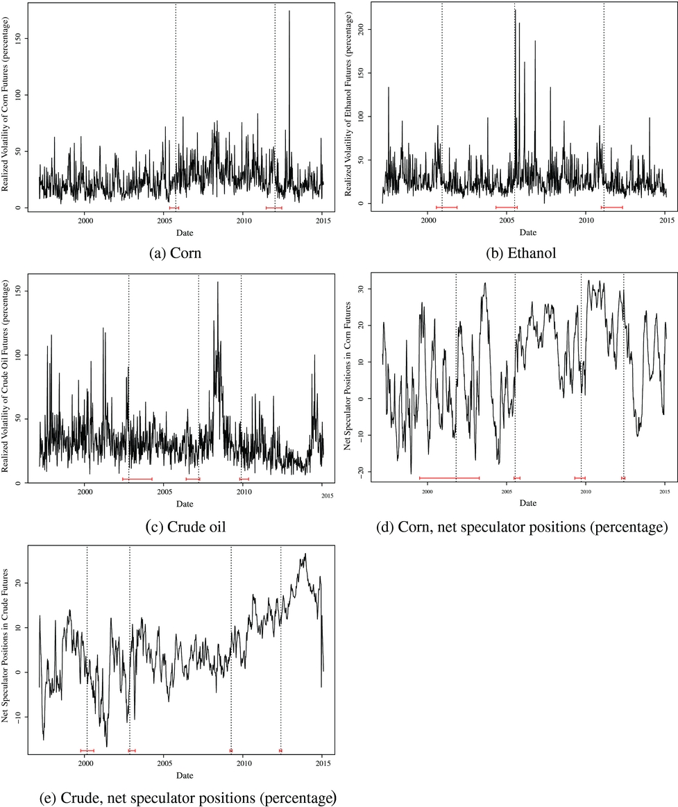
As a more precise test, we conducted the Qu and Perron (Reference Qu and Perron2007) test, which seeks to estimate one or more structural breaks that are common to all the variables within a multivariate regression. The Qu and Perron (Reference Qu and Perron2007) test was conducted, with code developed by the authors, using Gauss (version 17). (For the sake of brevity, the testing results are not provided here but are available upon request.) The unrestricted testing procedure of Qu and Perron (Reference Qu and Perron2007) estimates a common break point (of all variables within the system) around November of 2005—the 95% confidence interval for the break is estimated between the second week of November and fourth week of December 2005. Therefore, the Qu and Perron (Reference Qu and Perron2007) results seem to corroborate our approximate dividing of 2006, which we initially eyeballed based on the univariate Bai and Perron (Reference Bai and Perron2003) test procedures within Figure 1, so we split the overall sample period into two subperiods: 1997–2005 and 2006–2014. We experimented with splitting the sample at different dividing points using 2005 and 2007; however, the spillover results (not provided) were nearly identical. Intuitively, the common break (based on the Qu-Perron test) makes sense as the U.S. Energy Policy Act of 2005 was enacted in August of that year mandating domestic minimum biofuel production requirements, to be mixed with gasoline, in the United States (Dixon et al., Reference Dixon, McGowan, Onysko and Scheer2010).
As a sensitivity analysis, we further employed mean-comparison tests (multivariate analysis of variance [ANOVA] tests) to determine whether the means (of the separate price series) differ across the two subsample periods (1997–2005 and 2006–2014). The multivariate ANOVA test results, which are available upon request, imply that the average realized volatilities for corn, crude, and ethanol price series are statistically different across the two subsamples. The realized volatility of corn futures increased by more than 10%, on average, in the latter subsample (2006–2014), whereas the realized volatility in crude futures decreased by more than 5%. The realized volatility of ethanol futures also increased. These preliminary results imply that the increase in corn (future) price volatility is not attributable to increased volatility in oil prices as suggested by Balcombe (Reference Balcombe and Prakash2011).
Finally, diagnostic tests determine the best specification for the VAR model. A seasonal variable was included as the past literature has identified the presence of seasonality in agricultural commodity markets (Anderson, Reference Anderson1985; Karali and Thurman, Reference Karali and Thurman2010; Kenyon et al., Reference Kenyon, Kling, Jordan, Seale and McCabe1987; Yang and Brorsen, Reference Yang and Brorsen1993). In order to balance the trade-off between overparameterization (less lags specified) and autocorrelation (more lags specified), we selected a six-lag model. Our results indicated that a four-lag specification, although more parsimonious, led to some evidence of autocorrelation within the model; whereas the six-lag specification offered little to no autocorrelation within the model. Based on unit root test results, the six-lag specification resulted in weak stationarity within each of the endogenous variables within the system. The methodology we used within the current study is based on the model's forecasting ability, and by ensuring that the time series variables are weakly stationary, the forecasts should be far less susceptible to spurious inference. As a robustness check, we varied the lag length of the VAR and determined the estimates (in this case, the generalized forecast error variance decompositions) were insensitive to alternative lag specifications. Moreover, all cases contained stable characteristic roots.
We do not provide the 162 VAR coefficient estimates; we instead focus on the more useful spillover analysis based on the generalized forecast error variance decomposition. The atheoretical nature of VAR models is often criticized, so for validation we test the results against empirical reality (Freedman, Reference Freedman1991). Against this backdrop, our study focuses on the forecasts (error variance decomposition) provided by the VAR to better understand the spillover behavior among the commodities and the comparison of the rolling spillover plot with expected behavior relative to historical market activities.
5.2. Spillover Tables
The spillover tables for each subsample (1997–2005 and 2006–2014) are provided in Tables 3 and 4 and present an input-output decomposition of the spillover index (Diebold and Yilmaz, Reference Diebold and Yilmaz2009). The ijth entry in the table is the estimated contribution to the forecast error variance of variable i (denotes row entry) coming from innovations to variable j (denotes column entry) (Diebold and Yilmaz, Reference Diebold and Yilmaz2009). Put simply, the table's row elements represent a target variable, whereas the column elements represent a source shock. The off-diagonal column sums are labeled as “Contribution to others,” whereas the off-diagonal row sums are labeled as “Contribution from others.” The sum of either the columns or rows across variables yields the numerator in the spillover index. The column or rows sums, including diagonals, are labeled as “Contribution including own.” The sum of “Contribution including own” across variables yields the denominator of the spillover index.
Spillover Table for Subsample, 1997–2005

Notes: The underlying variance decomposition is based on a weekly vector autoregressive (VAR) of lag order 6, identified using the generalized VAR framework of Koop, Pesaran, and Potter (Reference Koop, Pesaran and Potter1996) and Pesaran and Shin (Reference Pesaran and Shin1998). All list variables include exogenous variables within the underlying VAR model. The exogenous variables include a constant and a weekly seasonal variable.
Spillover Table for Subsample, 2006–2014

Notes: The underlying variance decomposition is based on a weekly vector autoregressive (VAR) of lag order 6, identified using the generalized VAR framework of Koop, Pesaran, and Potter (Reference Koop, Pesaran and Potter1996) and Pesaran and Shin (Reference Pesaran and Shin1998). All list variables include exogenous variables within the underlying VAR model. The exogenous variables include a constant and a weekly seasonal variable.
In general, Table 3 does not reveal a great deal of volatility spillover among the three commodities (corn, crude oil, and ethanol). That is, own-historical volatility explains the largest portion of own-series error variance (80.91% for corn, 81.85% for crude, and 85.70% for ethanol). As Table 3 demonstrates, exchange rate volatility and volatility in the speculative positions for corn futures received the most influence from the other variables within the system at 25.9% and 23.9%, followed by volatility in corn futures prices and short-run interest rate volatility at 19.1% and 18.4%.
By comparing Table 3 and Table 4, we can remark about the difference in the results between the first and second subsample periods. The readers should use caution in ascribing causality in the volatility spillovers estimates. While comparing the two subsample periods, we analyze percentage changes in spillover estimates between periods; however, these changes do not necessarily represent causal changes to spillover activities across the two subsamples. Rather, the estimates here represent the percentage changes in how one commodity's volatility predicts another commodity's volatility, on average, across the subsample periods.
The difference in the estimates for the volatility spillover index (the total spillovers of volatility within the system) in the second subsample (2006–1014) is quite small; however, the discerning reader should keep in mind that the total volatility spillover measure is an average of spillovers (in volatility) among all the variables (within the system) over the entire subperiod sample. Hence, if the cross-commodity spillovers are relatively large while the spillovers in inventory levels are relatively small, then the estimate for the total volatility spillovers (within the system) will mask the cross-commodity spillovers.
As can be gleaned in Table 4, the volatility spillovers between the corn and crude commodities increased markedly in the second period. In particular, the volatility spillovers from crude to corn increased by approximately 46% [(0.036 − 0.0247)/0.0247], whereas the spillovers from corn to crude increased by approximately 181%. Our findings are qualitatively similar to that of Saucedo, Brümmer, and Jaghdani (2015) and Du, Yu, and Hayes (Reference Du, Yu and Hayes2011). This result suggests that, as corn price volatility explains more of crude price volatility and vice versa, the two commodities have become more integrated because of U.S. energy policies. This integration between corn and crude markets is consistent with the arguments (and/or findings) of Abbott (Reference Abbott2013) and Hertel and Beckman (Reference Hertel and Beckman2011). Further, the volatility spillovers from corn to ethanol increased by 376% from the first to second subsample period. Contrarily, the spillovers between ethanol and crude declined, demonstrating that it can be misleading to examine only the pairwise impacts between oil and ethanol or ethanol and corn as performed by Serra (Reference Serra2011). The increased transmissions (spillovers) among these commodities suggest perhaps a nontransitory integration of the markets.
To the casual reader, the changes may seem trivial. However, based on the average future contract price in corn, US$3.50 from 1997 to 2014, 5,000 bushels to a contract, and on average the daily number of open interest positions at nearly 1.5 million (U.S. Commodity Futures Trading Commission, 2009) while assuming that all the open interest positions are settled, a 1% difference in volatility is approximately equal to a change of US$125 million in the total (notional) market value of corn future contracts.
Despite the sizable implied increases, the cross-commodity spillovers still only account for a relatively small percentage in explaining the error variance of the individual volatility series. In the 2006–2014 subsample period, corn volatility only explains 5.9% of the total error variance of crude volatility, and crude volatility only explains 3.6% of the total error variance in corn volatility. Corn volatility explains a more substantial 11.42% of the total error variance of ethanol in the second subsample (Table 4). Similar to our study, Todorova, Worthington, and Souček (Reference Todorova, Worthington and Souček2014) found that cross-commodity spillovers provided useful incremental information in determining future price volatility; however, a commodity's own dynamics explain the largest portion of weekly volatility.
Our results suggest that the direct transmission from speculative positions to own price volatility decreased in the 2006–2014 subsample period by approximately 47% for crude and 86% for corn. The effect of speculative activities on inventory levels also seems to have changed over time. For the period 2006–2014, the results indicated substantial increases in spillovers from speculative corn activities to corn stocks-over-use by approximately 1,200% over the preceding subsample. Conversely, the transmission from net speculative positions in crude oil to crude inventory levels arguably decreased by nearly 83% in the second subsample. On the other hand, the transmission from net speculative position in crude oil to ethanol inventory levels arguably increased by roughly 300% in the second subsample period. Contrary to what was found in the earlier subsample, corn stocks-over-use played a less substantial role in explaining the speculative activities in corn in the second period. Put differently, the effect of corn inventory levels in predicting net speculator positions in corn decreased by approximately 32%. This finding implies perhaps that economic fundamentals (such as, inventory levels) now play a less substantive role in speculative activities. This could potentially reflect the increasing financialization of these commodity markets (Cheng and Xiong, Reference Cheng and Xiong2013).
Differing from the first subsample, speculation in crude oil futures and volatility in ethanol futures prices received the most contributions from others (30.7% and 24.2%, respectively), followed by corn (future) price volatility (23%) and crude oil (future) price volatility (19.3%). Our findings seem consistent with the narrative offered by Saghaian (Reference Saghaian2010), in which the early literature tended to focus on the exchange rate and how changes to monetary policies transmitted instability to agricultural prices; whereas, in more recent years the literature has evolved to examine the impacts associated with speculation and the links between energy and agricultural markets. For example, in the context of our findings, shocks to the exchange rate arguably played a much smaller role in predicting corn price volatility (from 3.77% in the 1997–2005 period to 1.66% in the subsequent 2006–2014 period).
5.3. Rolling-Window Spillover Index
Figures 2 and 3 demonstrate the rolling-sample spillover volatility index plots through time for each subsample, which provide an interpretation of the amount of volatility spillovers within the system through time for each subsample. For both of the figures, we used a 200-week rolling window (corresponding to about 4 years) with a 10-week-ahead forecasting horizon. The rolling spillover plot, labeled as “Total volatility spillovers,” is based on underlying VAR models with 12 variables (including the constant term and seasonality variable) and six lags specified. The “Total volatility spillovers” corresponds with the values estimated in the lower right-hand corner of each spillover table (similar to Tables 3 and 4). In other words, the top panel represents the total volatility spillovers (i.e., among all of the endogenous variables within our regression), followed by the directional (volatility) spillovers of crude oil to corn future prices, corn to crude oil future prices, ethanol to corn future prices, and corn to ethanol future prices. The vertical axes in Figure 2b–e are smaller than the index values of Figure 2a because the former are subsumed within the latter. (The same applies for Figure 3b–e.) Interpreted differently, the plots in Figure 2b–e correspond to the commodity-by-commodity spillover measures contained within Table 3—the only difference is the former are plotted against time based on the rolling regressions, whereas the latter represent an average over the entire subsample period. The astute reader will notice that the spillover plot diagram, Figure 2, is missing the first 4 years of data—this is attributable to the fact that the spillover plots are based on 200-week rolling windows (approximately 4 years); therefore, the spillover plots (which are based on ex post regression analyses) for the 1997–2005 subsample start in 2001.
Rolling Spillover Plots: 10-Week-Ahead Forecast Horizons, 1997–2005 (notes: spillover index plotted on vertical axis vs. time posted on horizontal axis; these plots demonstrate a moving volatility spillover index based on a 200-week rolling-window vector autoregressive [VAR] model with six lags specified; the shocks are defined according to the generalized forecast error variance decomposition derived from the estimated VAR)

Rolling Spillover Plots: 10-Week-Ahead Horizons, 2006–2014 (notes: spillover index plotted on vertical axis vs. time posted on horizontal axis; these plots demonstrate a moving volatility spillover index based on a 200-week rolling-window vector autoregressive [VAR] model with six lags specified; the shocks are defined according to the generalized forecast error variance decomposition derived from the estimated VAR)

The rolling-sample index plot for the total (system of equations) volatility spillovers, Figure 2a, demonstrates the largest spillover volatility occurred in 2003. This spike is consistent with the 2003 invasion of Iraq, which led to a decrease in Iraq's oil production and subsequently resulted in an average 19% increase (over 2002) in the price of a barrel of crude oil. As displayed in Figure 2b, this 2003 shock to global oil prices seems to have led to a peak in spillovers from crude oil price volatility to corn price volatility between 2004 and 2005. On the other hand, spillovers from volatility in corn prices to ethanol prices peaked in 2001 and then again in 2005 (as demonstrated in Figure 2e). Intuitively, this makes sense because California's ban on MTBE in 1999, coupled with the USDA's CCC Bioenergy Program in 2000, marks a turning point in the ethanol industry and introduces a link from the corn to the oil industry. However, corn price and crude oil price were not yet tightly integrated, so the increase in spillovers did not persist, and although ethanol capacity expands afterward, it is the (national) renewable fuel standard (RFS) created by the Energy Policy Act of 2005 that established the fundamental link between ethanol and corn markets.
The second rolling-sample index plots, for the 2006–2014 subsample in Figure 3a, suggest the largest spike in total volatility spillovers occurred in 2010, which corresponded with significant stock market volatility in the United States following the Great Recession (National Bureau of Economic Research, 2012). Opposite to the total (system) volatility spillover index, the spillover plots for each of the agricultural and energy commodity prices, Figure 3b–e, demonstrate a decline in volatility spillovers in 2010. This downward spike in spillovers is arguably attributable to the meteoric decline in crude oil prices, trading for more than $145 per barrel in July 2008 and falling to close to $40 per barrel by January 2009 (adjusted for inflation). Compared with the previous period, Figure 3b–e demonstrates more highly integrated spillover transmissions between the agricultural and energy commodities for the 2006–2014 subsample. For example, volatility spillovers from corn to ethanol prices showcase the highest increases as per the scaling of the vertical axis (the estimated contribution to the forecast error variance of ethanol volatility coming from corn volatility); Figure 2e represents estimated contributions ranging from 0 to 8% for the 1997–2005 subsample, whereas the vertical axis for Figure 3e represents estimated contributions ranging from 0 to 30% for the 2006–2014 subsample.
Similar to the arguments of Hertel and Beckman (Reference Hertel and Beckman2011) and Abbott (Reference Abbott2013), our estimated rolling (volatility) spillover index plots, Figure 3b–e, demonstrate increasing spillovers when higher oil price spikes in the first half of 2008 led to a nonbinding RFS, and decreasing volatility transmissions between crude and corn markets when the blend wall became binding in 2010. Based on the spillover volatility index, the agricultural and energy commodities behaved exactly as described by Abbott (Reference Abbott2013). That is, by 2010 U.S. ethanol production surpassed the blend wall and volatility spillovers decreased, but exports relieved pressure on ethanol production toward the end of the summer allowing for higher volatility spillovers (Abbott, Reference Abbott2013). As the subsidies to ethanol neared expiration and exports slowed, spillovers dropped (again, consistent with Abbott [Reference Abbott2013]), while the drought increased prices and volatility in the spring of 2012. By 2013, the U.S. Environmental Protection Agency, the agency responsible for administering the RFS2 program, acknowledged that the blend wall was officially binding production, and spillovers again dropped (consistent with Abbott's [Reference Abbott2013] observations). Capacity constraints, inventory conditions, and information assimilation in the markets accounted for finer changes and discrepancies in the spillover plot estimates.
6. Conclusions
Our study, by means of an estimated spillover table and rolling spillover index plots, demonstrates increasing volatility spillover transmissions in a system of corn (future) prices, crude oil (futures) prices, ethanol (futures) prices, interest rates, exchange rates, inventories, and speculation. Additionally, our findings suggest increasing cross-commodity volatility spillovers from crude oil to corn (future prices) and vice versa ceteris paribus for the period of 2006 to 2014. Our estimated spillover tables and rolling spillover index plots prove robust to the historical changes, based on policies and fundamentals, in spillover intensities. Moreover, our findings are consistent with the observations of Abbott (Reference Abbott2013) and Hertel and Beckman (Reference Hertel and Beckman2011).
Despite the large increase in volatility spillovers between corn and crude oil prices, which doubled, it is important to note that these cross-commodity (price) volatility spillovers still only constitute a relatively small portion of a commodity's total price volatility. Put differently, our results suggest that the influence from other sources, in the system of equations, to a commodity's volatility only increased slightly for corn price volatility (from 19% to 22.8%) and for volatility in crude oil prices (from 16.6% to 19.1%). Ethanol price volatility increased more substantially (from 14.4% to 25%). Further, although the spillover results arguably imply that biofuel policies have led to increasing spillovers from corn markets to crude oil and ethanol price volatility, they also indicate that other influences have led to an increasing volatility of crude oil prices.
In summation, the results of our empirical model imply relatively small volatility spillovers between corn, crude oil, and ethanol (in the range of 1%–12%) even after tremendous increases (i.e., doubling in some cases) in spillovers after 2006. Further, by utilizing a relatively large set of endogenous determinants of commodity price volatility, we also discovered that spillovers are not always direct, but may in fact be indirect. These findings might explain the contradictory estimates of volatility spillovers in prior studies.
Our study shows that the influence of inventory levels and macroeconomic conditions still warrants future research as also deduced from Serra and Gil (Reference Serra and Gil2013). Despite our study's contributions, the VAR model is atheoretical and only considers a system of simultaneously determined time series variables. Future research could perhaps offer a more rigorous theoretical analysis of the effect of competitive storage and market speculation on agricultural and energy commodity price volatility. Future research can also evaluate how volatility and other market interconnections will continue to change through time. Market dynamics can change with continuing pressure on the ethanol market because of blend wall limits, slowing growth in the ethanol industry since 2014, and persisting low crude oil prices, which are predicted to remain relatively low for the near term.
All the same, crude oil and grain commodity markets are expected to be more tightly integrated than in the preethanol era (independent of future energy policies or RFSs). Characteristically, ethanol is blended in gasoline not only to comply with policies like the RFS, but also to improve octane and to add to gasoline volume under favorable prices. Ethanol has become ingrained in the U.S. retail gasoline market over the past decades. For example, refineries now produce more unfinished gasoline specifically formulated for blending with ethanol to increase octane, and the majority of finished gasoline production has shifted from petroleum refiners to gasoline blenders. Moving finished product decisions for gasoline to blenders, rather than refiners, will arguably further increase the integration between crude oil and grain markets.
Of course, choices about the future direction of the RFS and fuel support will still play a critical role in shaping the biofuels industry and the integration of energy and agricultural markets. For example, enlarging ethanol use beyond the blend wall with higher blends (i.e., than the existing E10 standard) will likely result in increased spillovers between agricultural and energy markets. Conversely, future increases in cellulosic ethanol production will likely reduce integration between the markets. The impact of increases in drop-in fuels will depend on the biomass source but will in any case remove infrastructure barriers in blending and move the market biofuel market from mainly an oxygenate to a competitive gasoline volume market.


 Open access