Modelling the transition from grain-boundary sliding to power-law creep in dry snow densification

Elizabeth M. Morris; Lynn N. Montgomery; Robert Mulvaney

doi:10.1017/jog.2021.95

Modelling the transition from grain-boundary sliding to power-law creep in dry snow densification

Published online by Cambridge University Press: 08 September 2021

and

Elizabeth M. Morris*: Affiliation:
Scott Polar Research Institute, Lensfield Road, Cambridge CB2 1ER, UK
Lynn N. Montgomery: Affiliation:
Department of Atmospheric and Oceanic Science, University of Colorado, Boulder, CO, USA
Robert Mulvaney: Affiliation:
British Antarctic Survey, High Cross, Madingley Road, Cambridge CB3 0ET, UK
*: Author for correspondence: Elizabeth M. Morris, E-mail: emm36@cam.ac.uk

Article contents

Abstract
List of symbols
Introduction
The transition model
Data
Results
Discussion
Conclusion
Footnotes
References

Rights & Permissions

Abstract

This paper presents a physics-based macroscale model for the densification of dry snow which provides for a smooth transition between densification by grain-boundary sliding (stage 1) and densification by power-law creep (stage 2). The model uses established values of the stage 1 and 2 densification rates away from the transition zone and two transition parameters with a simple physical basis: the transition density and the half-width of the transition zone. It has been calibrated using density profiles from the SUMup database and physically based expressions for the transition parameters have been derived. The transition model produces better predictions of the depth of the nominal bubble close-off horizon than the Herron and Langway model, both in its classical form and in a recent version with re-optimised densification rates.

Keywords

Ice core polar firn snow physics

Information

Type: Article
Information: Journal of Glaciology , Volume 68 , Issue 269 , June 2022 , pp. 417 - 430

DOI: https://doi.org/10.1017/jog.2021.95 [Opens in a new window]
Creative Commons: This is an Open Access article, distributed under the terms of the Creative Commons Attribution licence (http://creativecommons.org/licenses/by/4.0/), which permits unrestricted re-use, distribution, and reproduction in any medium, provided the original work is properly cited.
Copyright: Copyright © The Author(s), 2021. Published by Cambridge University Press

List of symbols

DIP: depth-integrated porosity, m
E ₀: stage 1 activation energy, kJ mol⁻¹
E ₁: stage 2 activation energy, kJ mol⁻¹
H: depth of ice sheet, m
N: number of measurements
R: logarithmic function of density
R _s: polynomial curve fitted to R
R _model: model values of R
R _obs: observed values of R
T _m: mean annual firn temperature, °C or K
X: scaled density variable, a⁻¹
X ₀: surface value of X, a⁻¹
ā: mean annual accumulation rate, m w.e. a⁻¹
c: density-corrected volumetric strain rate, a⁻¹
k ₀: local stage 1 densification rate, m w.e.⁻¹
$k_0^\ast$: global stage 1 densification rate, m w.e.⁻¹
k ₁: local stage 2 densification rate, m w.e.⁻¹
$k_1^\ast$: global stage 2 densification rate, m w.e.⁻¹
q _T: water-equivalent depth at transition, m w.e.
z: height, m
z _T: transition height, m
z _s: smoothed profile height, m
z _BCO: bubble close off height, m
z _model: model height, m
A: parameter in transition model, a²
B: parameter in transition model, a⁻¹
C: parameter in transition model, a⁻¹
D: parameter in transition model, a⁻¹
M: parameter in transition model, kg² m⁻⁶ a²
R: gas constant, 8.314 J mol⁻¹ K⁻¹
ΔDIP: difference in depth-integrated porosity, m
Δz _BCO: difference in BCO height, m
Δρ: transition half-width, kg m⁻³
Γ: thinning function
Ψ: cost function
Ψ_min: minimum value of cost function
α: parameter in Herron and Langway equation
β: parameter in Herron and Langway equation
$\dot {\varepsilon }$: volumetric strain rate, a⁻¹
$\dot {\varepsilon }_{\rm H}$: horizontal flow divergence, a⁻¹
$\dot {\varepsilon }_{zz}$: vertical strain rate, a⁻¹
λ: length scale, m
ρ: mean density over a macroscale element, kg m⁻³
ρ′: variable density within a macroscale element, kg m⁻³
ρ ₀: surface intercept density, kg m⁻³
ρ ₁: lowest density in optimisation range, kg m⁻³
ρ ₂: highest density in optimisation range, kg m⁻³
ρ _T: transition density, kg m⁻³
ρ′_T: variable transition density within a macroscale element, kg m⁻³
ρ _i: density of ice, kg m⁻³
ρ _w: density of water, kg m⁻³
ρ _BCO: nominal bubble close off density, kg m⁻³
σ: overburden stress, Pa
τ: time from deposition, a
τ _T: time from deposition to transition, a
θ _BCO: thinning correction at bubble close off, m
ɛ_T: total strain to transition

1. Introduction

Models of the densification of dry snow are used for a wide range of glaciological and meteorological purposes, including, for example, predicting the energy budget at the lower boundary of the atmosphere in climate models, predicting the formation of weak layers in avalanche models, interpretation of seismic and radar-sounding data and derivation of age–depth relations for firn cores. In particular, two key problems are often identified as drivers for the development of firn densification models. The first concerns the interpretation of altimetry data, in particular the satellite data which have revealed the response of the polar ice sheets to recent climate change. A change in elevation of an element of the ice-sheet surface can occur both because of a change in the mass of the underlying ice and firn column and because of a change in its depth-integrated porosity (DIP). A model is needed to predict how DIP will vary with changing climate before elevation changes can be linked to mass-balance changes. The second problem concerns the interpretation of ice core palaeoclimate and atmosphere data. The age of gas bubbles in an ice core segment will not be the same as the age of the surrounding ice because the gas is able to move while in the porous firn region. Estimating the age difference, so that climate variables deduced from the gas and ice chemistry can be reconciled, requires a densification model to predict bubble close-off (BCO) depth in the firn.

Snow densification models range from the relatively simple linear viscous approximations used in seasonal snow cover models (e.g. Brun and others, Reference Brun, Martin, Simon, Gendre and Coleov1989; Jordan, Reference Jordan1991; Bader and Weilenmann, Reference Bader and Weilenmann1992) to more complex formulations based on details of physical processes at the grain-size scale (e.g. Salamatin and others, Reference Salamatin2009; Fourteau and others, Reference Fourteau, Gillet-Chaulet, Martinerie and Fan2020). In many applications the input data are limited, and this in turn limits the complexity of the models that can be used. One widely used model developed by Herron and Langway (Reference Herron and Langway1980) defines densification rates at a given site simply in terms of the mean annual firn temperature, T _m, mean annual accumulation, ā, and surface intercept density, ρ ₀. This may be regarded as the ‘common ancestor’ (Lundin and others, Reference Lundin2017) of a number of other macroscale models that rely on similar input data and share common assumptions about the densification process.

One of these assumptions is that snow densification occurs first by rearrangement of the ice grains to produce a closer packing. The grains move by sliding at their boundaries until the closest possible packing is achieved, at which point further densification is only possible by plastic deformation of the grains themselves. This power-law creep continues until the pores in the matrix are enclosed and further densification then depends on compression of the gas in the bubbles. The Herron and Langway (Reference Herron and Langway1980) model defines a fixed transition density for all sites, ρ _T, between the first and second stages of densification, as 550 kg m⁻³. This value is physically plausible, since it lies between the densities of the loosest (479 kg m⁻³) and closest (679 kg m⁻³) theoretical packing of ice spheres (Benson, Reference Benson1962), and has continued to be used in current models (e.g. Barnola and others, Reference Barnola, Pimienta, Raynaud and Korotkevich1991; Spencer and others, Reference Spencer, Alley and Creyts2001; Goujon and others, Reference Goujon, Barnola and Ritz2003; Arthern and others, Reference Arthern, Vaughan, Rankin, Mulvaney and Thomas2010; Ligtenberg and others, Reference Ligtenberg, Helsen and van den Broeke2011; Simonsen and others, Reference Simonsen2013; Verjans and others, Reference Verjans2020).

Nevertheless, the possibility that ρ _T is not a constant was raised early in the development of densification models. On the somewhat uncertain basis of four density profiles, Benson (Reference Benson1962) derived an empirical expression in terms of T _m which implies a maximum value of 730 kg m⁻³ at 0°C and a minimum value of 500 kg m⁻³, no matter how cold the snow becomes. He suggested near-zero temperatures favour stage 1 densification because the formation of a liquid layer at the grain-boundaries allows this stage to continue to a greater density. Arnaud and others (Reference Arnaud, Lipenkov, Barnola, Gay and Duval1998) agreed that the transition density decreases with temperature; their explanation was that the overburden stress, σ, at the transition is greater at cold sites, so that densification by creep (∝ σ ³) is favoured over densification by grain-boundary sliding (∝ σ) and can begin at a lower density.

The idea that stages 1 and 2 are separated by an abrupt transition was challenged early on by Ebinuma and Maeno (Reference Ebinuma and Maeno1987) who suggested that particle rearrangement and plastic creep can operate together over a wide transition region from 550 kg m⁻³ to ~700 kg m⁻³. These densities were deduced from ice core data at relatively low resolution (spacing ≥ 50 cm). Higher resolution profiles reveal the variation in density between and within annual layers and have led to a more detailed understanding of the physical processes controlling densification in dry polar snow. In particular, Gerland and others (Reference Gerland1999) and Freitag and others (Reference Freitag, Wilhelms and Kipfstuhl2004) showed that initially lower-density, coarse grained, ‘summer firn’ layers had a higher stage 1 densification rate than initially higher-density, fine-grained ‘winter firn’ and Hörhold and others (Reference Hörhold2012) showed that a variation in impurity concentration could produce a variation in stage 2 densification rates. This variability in both density and densification rates will broaden the range over which the transition from stages 1 to 2 appears to occur on the macroscale, that is when we consider the smoothed density profile rather than details of the annual layering.

The concept of a transition zone was incorporated into the Herron and Langway model by Morris (Reference Morris2018). The ‘Morris transition model’ removes the abrupt transition between stage 1 and stage 2 densification at a fixed transition density and includes two optimisable parameters. These are the transition density, ρ _T, and the transition half-width, Δρ, a measure of the density range over which the transition occurs. Early values of these parameters were determined by examination of short strain rate profiles from the Pine Island Glacier basin, Antarctica (Morris and others, Reference Morris2017). This paper extends that work using 103 profiles from the SUMup community dataset of snow and firn density (Montgomery and others, Reference Montgomery, Koenig and Alexander2018). We develop new, physically based, expressions for the transition parameters and assess the performance of the model in terms of its ability to predict the nominal BCO depth for 45 of the profiles.

2. The transition model

The transition model is based on the Robin hypothesis that, in dry snow, the volumetric strain rate, $\dot {\varepsilon }$, is related to the (macroscale) density ρ by the expression

(1)$$\dot{\varepsilon} = c\left({\rho_{\rm i}-\rho\over \rho}\right),\; $$

where ρ _i is the density of ice. The density-corrected volumetric strain rate, c, is written

(2)$$c = \left(\rm{D} + {\it{X}\over \rm{\vert( 1 + A} \it{X}\rm{^2) ^{1/2}\vert}}\right),\; $$

where A and D are constants and X = (ρ − ρ _T)/M^1/2 is a scaled density variable describing distance from the transition density ρ _T. Away from the transition c tends to the stage 1 and stage 2 constant density-corrected strain rates. That is, for $\rm{A}\it{X}\rm{^2} \gg$ 1, c → (D − A^−1/2) or (D + A^−1/2). Parameter M controls the abruptness of the transition. The half-width of the transition, Δρ, is defined by the points where c reaches 90% of its stage 1 and stage 2 values, that is

(3)$$\eqalign{ \rho & = \rho_{\rm T} - \Delta\rho \quad \rm{\,for} \quad \it{c} = \rm{0.9 \left({D} - {A}^{-1/2}\right)},\; \cr \rho & = \rho_{\rm T} + \Delta\rho \quad \rm{\,for} \quad \it{c} = \rm{0.9 \left({D} + {A}^{-1/2}\right)},\; }$$

from which

(4)$$\Delta\rho \approx 2.06 \left({\rm{M}\over {A}}\right)^{1/2}.$$

For constant ā, we can derive an expression relating height, z, (positive upwards) and scaled density X:

(5)$$\eqalign{\int {\rm d}z & = {\bar{a}\over {\rm M}^{1/2}} \cr & \quad\times\int {( 1 +{ \rm A} X{^2}) ^{1/2} {\rm d}X\over \left({\rm D}( 1 + {\rm A} X{^2}) ^{1/2} + {X}\right)\left({\rm C}-X\right)\left(X-{\rm B}\right)},\; }$$

where B = −ρ _T/M^1/2 and C = (ρ _i − ρ _T)/M^1/2. Equation (5) allows us to calculate the depth at which any given density is reached, for example the nominal BCO depth, − z _BCO, at which ρ = ρ _BCO. There is evidence (Martinerie and others, Reference Martinerie1994) that the (macroscale) BCO density varies with climate, in particular increasing from ≈815 kg m⁻³ at − 15°C to ≈ 834 kg m⁻³ at − 55°C. In this paper, we set a nominal value ρ _BCO = 815 kg m⁻³, following the example of the FirnMICE intercomparison of densification models (Lundin and others, Reference Lundin2017).

The model also leads to an analytic solution for the depth-integrated porosity

(6)$$\eqalign{ DIP & = \displaystyle\int_z^0 {\left(\rho_{\rm i}-\rho\right)\over \rho_{\rm i}} {\rm d}z \cr & = {\bar{a}\over \rho_{\rm i}}\displaystyle\int_{X}^{X_0} {\left(1 +{ \rm A} {X}^2\right)^{1/2}{\rm d}X \over \left({\rm D} \left(1 + {\rm A} X^2\right)^{1/2} + X\right)\left(X-{\rm B}\right)},\; }$$

where X ₀ is the surface value of X. The water-equivalent depth at BCO is simply ρ _i( − z _BCO − DIP _BCO) and hence the BCO age may be calculated using the mean annual accumulation and Eqns (5) and (6). Analytical solutions for the integrals in these equations are given in Morris (Reference Morris2018).

As it stands the model has four parameters, all of which could be tuned to obtain the best fit to strain rate or density profiles. In order to pin down the effect of adding the two transition parameters, we choose to fix D and A so that $( {\rm D - A}^{-1/2}) = -\bar {a}k_0$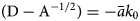 and $( {\rm D + A}^{-1/2}) = -\bar {a} k_1$ 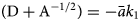where k ₀ and k ₁ are the local stage 1 and stage 2 densification rates defined by Herron and Langway (Reference Herron and Langway1980). They are related to global rates $k^\ast _0$ and $k^\ast _1$ by Arrhenius expressions

(7)$$k_0 = k^\ast _0 \bar{a}^{\left(\alpha-1\right)}\exp\left({-E_0\over {{\rm R}}T_{\rm m}}\right)$$

and

(8)$$k_1 = k^\ast _1\bar{a}^{\left(\beta-1\right)} \exp\left({-E_1\over {\rm R}T_{\rm m}}\right).$$

Here, R = 8.314 J mol⁻¹ K⁻¹ is the gas constant, T _m is in degrees Kelvin and the stage 1 and 2 activation energies are E ₀ = 10.16 kJ mol⁻¹ and E ₁ = 21.40 kJ mol⁻¹ respectively. Herron and Langway (Reference Herron and Langway1980) set α = 1 and β = 0.5 so that only k ₁ is dependent on ā. In this case, the global vertical densification rates for stages 1 and 2 are $k^\ast _0 = 11$ m w.e.⁻¹ and $k^\ast _1 = 575$ m w.e.^−1/2 a^−1/2 respectively. Note that, for very low accumulation, these values can lead to the unrealistic situation of k ₁ > k ₀.

This classical Herron and Langway model, which we shall refer to as the HL model, may be regarded as a benchmark model for dry snow densification (Lundin and others, Reference Lundin2017). Other researchers have since adapted the expressions for the densification rates; in particular, Verjans and others (Reference Verjans2020) have derived an optimal set of the six parameters in Eqns (7) and (8) by minimising the difference between observed and predicted values of the variable [DIP(ρ = 830 kg m⁻³) − DIP(z = −15 m)] for a sub-set of the SUMup density profiles taken as a whole. The Verjans version of the Herron and Langway model, HL(V), can be taken as an example of the improvement that can be made by adjusting the densification rates while retaining an abrupt transition. However, we note that the HL(V) parameters were obtained using climate forcing from a regional climate model, rather than mean annual values T _m and ā.

By fixing k ₀ and k ₁ at the HL values, we can compare the improvement in model predictions produced by inclusion of a transition zone with that produced by optimisation of the densification rates. In this paper, we shall refer to this version of the transition model as HL(T). A similar exercise could, of course, be undertaken for other models with an abrupt transition.

In Morris (Reference Morris2018) the transition parameters of HL(T) were optimised to obtain the best fit to measured strain rate profiles using Eqns (1) and (2). However, few such strain rate data are available. Density profile data, on the other hand, are available for a wide range of climatic conditions. We therefore optimise ρ _T and Δρ to obtain the best fit to profile data using Eqn (5). Specifically we seek the best fit to observed profiles, R _obs, of the logarithmic function

(9)$$R = \ln \left({\rho\over \left(\rho_{\rm i} - \rho\right)}\right).$$

Since we are interested in the transition region, we optimise over the range ρ ₁ = 500 kg m⁻³ to ρ ₂ = 700 kg m⁻³, unless the record is too short, or the data are too sparse, to make this feasible, in which case the range is adapted slightly. We define a cost function which can be applied to density data with widely differing resolutions and numbers of points in the optimisation range. This is achieved by fitting a third-order polynomial R _s to R _obs so that N height values, z _s(i), for the smoothed profile can be calculated at regular intervals of 5 kg m⁻³ from ρ ₁ (i = 1) to ρ ₂ (i = N). Model heights, z _model(i), are calculated at the same intervals. The constant of integration in Eqn (5) is defined so that R _model = R _s at density ρ ₁ and ρ _model = ρ ₀ at the surface z = 0. Given that Eqn (7) does not apply to the near-surface layer with its strongly varying temperature, the model surface intercept density, ρ ₀, will not necessarily be the same as the observed surface density.

The cost function, Ψ, is defined as

(10)$$\Psi = \left({1\over N} \sum_{i = 1}^N \left({\left(z_{\rm model}( i) -z_{\rm s}( i) \right)\over z_{\rm s}( i) },\; \right)^{2} \right)^{1/2}$$

and the optimum values of ρ _T and Δρ for a given profile (i.e. the local optimum values) are those that minimise Ψ for that profile.

In order to develop physics-based equations for global values of the transition parameters we need to consider the length scale, λ, of HL(T). The model predicts the mean density ρ over a macroscale element of length λ, that is, the mean of the varying density ρ′ within it. We can split the variation into two parts: first the annual and sub-annual fluctuations of amplitude ≈ 50 kg m⁻³ apparent in high-resolution density profiles (e.g. Hörhold and others, Reference Hörhold, Kipfstuhl, Wilhelms, Freitag and Frenzel2011) and secondly the slow increase in density from the upper part of the element to the lower part. This will not always be negligible. For a densification rate of 0.05 m w.e. a⁻¹ and density 500 kg m⁻³, for example, the increase would be ≈ 10 kg m⁻³ for λ = 1 m.

Within the macroscale element there may also be a variable transition density ρ′_T because some layers of the snow are weaker than others. Some of this variability will be annual and sub-annual, but some will be on a longer timescale. For example, there may be a run of several years with high dust concentration which increases the stage 2 creep rate (Hörhold and others, Reference Hörhold2012), followed by several years with lower levels. The choice of λ has to be such that this variability is smoothed on the macroscale.

Now we consider what happens as an element of length λ moves downwards from the surface. Given a fixed value of ρ′_T, the macroscale transition zone must extend from the point where the first density peak in the element reaches this value to the point where the last density trough passes it. Thus, a minimum value of the macroscale transition half-width, Δρ, is given by the amplitude of ρ′. A similar argument can be used to determine the effect of varying ρ′_T with fixed ρ′. The minimum value of Δρ is given by the amplitude of ρ′_T. When the two effects are combined, the minimum value of Δρ is the greater of the two amplitudes. However, it is also the case that the transition zone has to extend for at least a half-cycle in density or strength i.e. from density peak to density trough or from strength trough to strength peak. This implies $\Delta \rho \gtrapprox -k_0 \rho ( \rho _{\rm i} -\rho ) \lambda /4$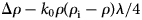 which for large λ may become greater than the amplitudes of ρ′ and ρ′_T.

For low-accumulation sites, Δρ will be controlled by the amplitude of the annual and sub-annual density fluctuations and the transition region will extend over many annual layers. In this case the length scale of the model can be much less than the width of the transition zone. However, for high-accumulation sites the length scale required to smooth the fluctuations controls the transition width and the two are of the same magnitude. At this stage, if λ extends over a fixed number of annual layers, a linear relation will develop between Δρ and ā.

3. Data

3.1. Profiles used in this study

We have divided the snow density profiles available from the 2020 SUMup database (Montgomery and others, Reference Montgomery, Koenig and Alexander2018), plus some new profiles yet to be added to SUMup, into groups, depending on the resolution of the data, the length of the record and our judgement of the accuracy of the associated climate data (Appendix A).

At 29 sites very high-resolution density profiles have been obtained using gamma-ray attenuation techniques (Wilhelms, Reference Wilhelms1996; Breton and others, Reference Breton, Hamiliton and Hess2009) to depths well below the transition from stage 1 to stage 2 densification at z _T (Table A1). The mean annual accumulation has been determined by chemical analysis of the core and the mean annual firn temperature has been measured at the site. A further 21 density profiles (Table A2) were collected using a neutron-scattering technique (Morris and Cooper, Reference Morris and Cooper2003). These data have a reasonably high resolution of ≈ 3 cm, and T _m and ā have been measured in situ. The Katie profile, from a borehole near Summit Station, Greenland, is 30 m long and covers the whole of the transition region. However, the diameter of the hole was relatively large (nominal value 14.9 cm) so there is a risk of error in the calculated density if the 5 cm diameter neutron probe moved from its correct position resting on the wall of the hole. The remaining profiles, collected during the iSTAR traverse across Pine Island Glacier, Antarctica, were obtained from 5 cm access holes, so this problem did not arise. They are short (13 m), and therefore may not cover the whole of the transition region, but useful because (1) they cover climatic conditions for which gamma-ray profiles are not available, (2) because some of the profiles come from regions of unusually high velocity divergence and (3) because there are gravimetric measurements from many of the same sites so a comparison between measurement techniques can be made.

Gravimetric density profiles longer than 50 m have been divided into three groups. We have found 14 profiles for which the average data resolution is <50 cm and the climatic data have been measured in situ (Group A, Table A3) and 22 sites with average data resolution >50 cm but with good in situ climate data (Group B, Table A4). We have added gravimetric data from the Katie core to Group B, although the record is only 30 m long, because this is the only site for which we have both neutron scattering and gravimetric data from exactly the same spot. Finally, we have 17 lower-resolution sites (Group C, Table A5) with data which need special attention. This may be because in situ climate data are not available or because we believe errors have arisen in transferring climate data from the primary sources to existing databases.

To avoid over-loading Tables A1 to A5, site positions, citations and comments on any changes we have made are given in the Supplementary material to this paper.

3.2. Excluded profiles

There remain a few profiles used in other studies which fall within our general criteria but which are excluded from this study. Two sites (Dominion Range and Newall) have very low accumulation rates for which the Herron and Langway (Reference Herron and Langway1980) theory breaks down (because the calculated values of k ₁ is greater than the calculated value of k ₀). The density profile from Prospector-Russell Col, Mount Logan (personal communication from D. A. Fisher, 2020) does not show a change in the observed densification rate, so that stage 1 cannot be distinguished from stage 2. The same is true of the Upstream B profile (important in the development of densification models as it demonstrated the effect of stress-enhancement on stage 2 creep (Alley and Bentley, Reference Alley and Bentley1988)). Profiles JARE and JARE11 have anomalously high densities and an apparent hiatus in snow accumulation, perhaps caused by katabatic winds (Kameda and others, Reference Kameda, Shoji, Kawada, Watanabe and Clausen1994). Profiles from Taylor Dome and Law Dome (Dome Summit South, DSS) do not have good density data near the surface. The profile from Site 2, an early US coring site in Greenland, shows an oscillation in density with depth which obscures details of the transition from stages 1 to 2. The accumulation rate for Mizuho S25 given by Spencer and others (Reference Spencer, Alley and Creyts2001) comes from a personal communication and may be incorrect. The accumulation rate quoted for Ridge B-C comes from a stratigraphic study over 7 years and is not necessarily the long-term average. This leaves us with 103 profiles, of which 12 were selected by Spencer and others (Reference Spencer, Alley and Creyts2001) to calibrate their model, eight were selected by Verjans and others (Reference Verjans2020) and a further three were used in both studies.

3.3. Climatic distribution of the data

Figure 1 shows the climatic distribution of the data. The gamma-attenuation data span the whole range of T _m and ā, but there are gaps to be filled. The neutron-scattering data fill in the gap between −25 and − 20°C but between −40 and − 33°C we have to rely on one Group B point (BAS M1) and one Group C point (Mizuho G15). Two Group B points (Dome C and ITASE02_6) fill the gap between −55 and − 46°C. The gap between 0.8 and 1.2 m w.e. a⁻¹ is filled by one Group B point (Beethoven Peninsula) and one Group C point (DE08). We use the colour coding introduced in Figure 1 to distinguish the different groups in subsequent figures.

Fig. 1.

Distribution of density profiles used in this study with mean annual temperature, T _m, and mean annual accumulation, ā. The profiles are divided into groups according to the measurement techniques used (gamma-ray attenuation (γ), neutron scattering (np) and gravimetric (grav.)) and the quality of the data (A, B, C). Above the dashed line the Herron and Langway (Reference Herron and Langway1980) stage 1 densification rate is greater than the stage 2 rate.

All of the profiles can be used to estimate local values of the transition parameters ρ _T and Δρ, although the high-resolution data are expected to give higher precision. The number of profiles which can be used to test the ability of the model to predict z _BCO or DIP is more limited; there are 17 that are long enough in the gamma-attenuation group, 3 in Group A, 16 in Group B and 11 in Group C, a total of 45. We have found reliable corrections for thinning for only 15 of these. Thus, despite the large number of density profiles now available from the SUMup database, we are still somewhat limited in what can be achieved by their analysis.

4. Results

As an example of the results, Figure 2 shows the observed and modelled profiles for core B36/B37 collected at the EPICA deep drilling site in the interior of Dronning Maud Land (EDML) where T _m = −44.6°C and $\bar {a} = 0.067$ m w.e. a⁻¹. The best fit across the transition region is obtained with ρ _T = 509 kg m⁻³ and Δρ = 39 kg m⁻³ (Table A1). In the upper 10 m of the profile, the HL(T) curve follows the HL stage 1 curve. The densification rate then decreases for ~10 m until the stage 2 rate is reached. The amplitude of the observed density variability decreases with depth, to a minimum just below the transition zone, and then increases through the stage 2 region. Thus this profile displays the ‘cross-over process’ where through the transition region the densest layers densify at approximately the stage 2 rate, whereas the least dense layers continue to densify at the stage 1 rate (Gerland and others, Reference Gerland1999; Freitag and others, Reference Freitag, Wilhelms and Kipfstuhl2004). The value of Δρ reflects the amplitude of the density fluctuations. Using the mean annual accumulation rate of $\bar {a} = 0.067$ m w.e. a⁻¹ we calculate that the transition occurs over a period of ≈70 years, so that a relatively large number of annual layers are involved.

Fig. 2.

Observed and modelled profiles of R = ln(ρ/(ρ _i − ρ)) for core B36/B37. The very high-resolution density data R _obs were collected using a gamma-ray attenuation technique. Horizontal dotted lines show the extent of the transition region from stage 1 to stage 2 densification, that is, ρ _T ± Δρ, and the nominal transition to stage 3. The extended HL stage 1 and 2 curves cross at 550 kg m⁻³. The parameters of the transition model HL(T) are optimised to produce the best fit to R _s, which is a polynomial fit to the observed data across the transition region.

Because ρ _T is <550 kg m⁻³, the transition model can produce an improved fit by lowering the model densities, without changing the HL stage 2 rate. The difference between the BCO heights predicted by the HL(T) and HL models is Δz _BCO = −2.471 m, that is, the transition model predicts a deeper BCO horizon. In fact Figure 2 shows there is a constant horizontal offset of − 2.471 m between the HL(T) model curve and HL stage 2 curve for all depths below the transition region. The transition model gives DIP = 33.144 m whereas the HL model predicts DIP = 32.062 m. Thus the difference in depth-integrated porosity is ΔDIP = 1.082 m. Note however that both models will under-estimate DIP because they use mean annual temperature and do not take account of increased densification rates in the surface layer of snow affected by the annual temperature variation.

Although the HL(T) model appears to produce a good estimate of the nominal BCO depth, we note that this is because the observed densification rate is slightly lower than the HL rate for the upper part of stage 2 and then slightly higher in the lower part. This may indicate that there is a gradual transition between stage 2 and stage 3 densification, beginning at a density <815 kg m⁻³. However, in this paper we focus on modelling the stage 1/stage 2 transition and retain the single nominal value of ρ _BCO = 815 kg m⁻³ so that our results can be compared with those of the Firn Model Intercomparison Experiment (FirnMICE) (Lundin and others, Reference Lundin2017).

Figure 3 shows observed and modelled profiles for a contrasting example. Core B38 was collected at the summit of Halvfarryggen, a small ice dome in coastal Dronning Maud Land, where T _m = −18.1°C and $\bar {a} = 1.250$ m w.e. a⁻¹ (Table A1). The best fit over the transition region is obtained with ρ _T = 549 kg m⁻³, very close to the HL transition value of 550 kg m⁻³. However, Δρ = 135 kg m⁻³ and the transition region begins at the surface and extends for ≈ 30 m. This allows the HL(T) model to produce a better fit to the observed data by raising the model densities without changing the HL stage 2 rate. In this case Δz _BCO = 13.689 m and ΔDIP = −4.201 m, that is the transition model predicts a shallower BCO horizon and a decreased value of DIP. Again, we note that the HL(T) and HL model values of DIP, 27.262 and 31.463 m respectively, will be under-estimates of the true value.

Fig. 3.

Observed and modelled profiles of R = ln(ρ/(ρ _i − ρ)) for site B38. The very high-resolution density data R _obs were collected using a gamma-ray attenuation technique. Horizontal dotted lines show the extent of the transition region from stage 1 to stage 2 densification, that is, ρ _T ± Δρ, and the nominal transition to stage 3. The extended HL stage 1 and 2 curves cross at 550 kg m⁻³. The parameters of the transition model HL(T) are optimised to produce the best fit to R _s, which is a polynomial fit to the observed data across the transition region.

The amplitude of the density fluctuations in the upper part of this profile is less than half of the optimised value of Δρ, suggesting that in this case the scale length λ has become the controlling factor. Using the mean annual accumulation rate of $\bar {a} = 1.25$ m w.e. a⁻¹ we calculate that the transition occurs over a period ~10 years, suggesting decadal variations in ρ′_T. A dust concentration profile for B38 is available (Schmidt and others, Reference Schmidt2014) and shows both annual and multi-year variability. This may be the explanation for the variations in ρ′_T. However, we note also that, if the actual stage 2 densification rate is higher than the HL rate, the value of Δρ will have to increase to compensate and vice versa. Thus Δρ could also include a component arising from uncertainty in $k_1^\ast$.

In both these examples the fit below the transition region would be improved by optimising the stage 2 densification rate or even allowing it to vary with depth. However, our object is not to produce the best possible simulation of individual profiles, but rather to gain insight into how we might derive global values of ρ _T and Δρ and to quantify the improvement produced by incorporating them into the HL model. These are therefore the only parameters we allow to vary.

For individual profiles, the goodness-of-fit in the transition region is given by the cost function Ψ. Figures showing the variation of Ψ with ρ _T and Δρ are given in the Supplementary material for sites B36/B37 and B38. In both cases there is a simple minimum and Ψ is more sensitive to ρ _T than Δρ. For B36/B37, Ψ_min = 0.0124 and ∂Ψ/∂ρ _T ≈ 3∂Ψ/∂Δρ. For B38, Ψ_min = 0.0093 and ∂Ψ/∂ρ _T ≈ 4.5∂Ψ/∂Δρ. In general, values of Ψ_min range from 0.0034 for the Vostok profile (Table A5) to 0.1784 for DML96C07_39 (B39) (Table A1).

4.1. Estimation of the uncertainty in model parameters

Two profiles were obtained from exactly the same point at the Katie site near Summit Camp, Greenland. A core was extracted and segments weighed to provide a gravimetric profile, and the resulting borehole was profiled using a neutron probe. The value of ā was derived by counting annual density peaks for the neutron scattering profile and by chemical analysis of a range of seasonally varying elements for the gravimetric profile (Hawley and others, Reference Hawley, Morris and McConnell2008) leading to two slightly different values, 0.216 m w.e. a⁻¹ and 0.23 m w.e. a⁻¹ respectively. In this particular case we have the opportunity to assess the uncertainty in the optimised values of the model parameters arising from the use of different measurement techniques. The differences in best estimates for ρ _T, Δρ and ρ ₀ are 14, 19 and 15 kg m⁻³, respectively (Tables A2 and A4). An increase in Δρ is accompanied by a decrease in ρ _T.

Pairs of profiles were also obtained at 10 sites along the iSTAR traverse across Pine Island Glacier, Antarctica. Cores were extracted close to boreholes where neutron probe profiles had been obtained the previous year (Tables A2 and A3). These data allow the effect of local spatial variability plus different measurement techniques to be assessed. Figure 4 shows that the optimum values of ρ _T for each site differ by 10 kg m⁻³ or less; slightly less than the difference of 14 kg m^-3 found at the Katie site, where the neutron scattering profile is likely to be less accurate than those from the iSTAR sites.

Fig. 4.

Best value of ρ _T from neutron scattering density profiles at 10 iSTAR sites as a function of the best value from gravimetric profiles nearby. The solid line shows a 1:1 relationship and dotted lines indicate an uncertainty of ± 10 kg m⁻³.

Figure 5 shows that the optimised values of Δρ for each site differ by up to 40 kg m⁻³, with the neutron scattering values tending to be greater than the gravimetric values. This is because the neutron scattering profiles are short and do not define the extent of the transition zone as accurately as the longer gravimetric profiles. Finally Figure 6 shows that the values of ρ ₀ chosen for the two profiles at each site differ by up to 7 kg m⁻³. If there is any error in matching the observed and modelled curves at density ρ ₁ to determine the constant of integration (Section 2), this will affect best estimates of ρ ₀ and ρ _T in the same way. We find no correlation between [ρ ₀(gravimetric) − ρ ₀(np)] and [ρ _T(gravimetric) − ρ _T(np)] so conclude that this potential systematic error is not important.

Fig. 5.

Best value of Δρ from neutron scattering density profiles at 10 iSTAR sites as a function of the best value from gravimetric profiles nearby. The solid line shows a 1:1 relationship and dotted lines indicate an uncertainty of ± 40 kg m⁻³.

Fig. 6.

Best value of ρ ₀ from neutron scattering density profiles at 10 iSTAR sites as a function of the best value from gravimetric profiles nearby. The solid line shows a 1:1 relationship and dotted lines indicate an uncertainty of ± 7 kg m⁻³.

We proceed on the assumption that ≈ ±10 kg m⁻³ is a reasonable estimate for the uncertainty in optimised values of ρ _T and ρ ₀ for all the profiles and estimate the uncertainty in Δρ as ≈ ±40 kg m⁻³ for the short iSTAR neutron scattering profiles and ≈ ±20 kg m⁻³ for the longer profiles. To set these estimates in context we note that the expected random error in the neutron probe density measurements is $\approx 2\%$ and the systematic error arising from a 5% error in borehole diameter would be a further 2% (Morris and Wingham, Reference Morris and Wingham2014). With these uncertainties we can see from Table 1 that the optimised values (which cannot be negative) are consistent for the pair of profiles B36/B37 and BAS ISOL (both from the EDML site at Kohnen Station), for the pair of profiles B25 and T1 (separated by 5 km on Berkner Island) and for the pair of profiles WDC06A and ITASE00_1 (separated by 21 km on the WAIS Divide). The climate parameters for each pair are the same, or very similar. The two sites from the Dyer Plateau have not been included in Table 1 because there is a significant difference in mean annual accumulation, despite their proximity.

Table 1.

Optimised parameters for profile pairs

4.2. Surface intercept density

Figure 7 shows the surface intercept density generally increases with mean annual temperature and accumulation, as expected. However, within the temperature range of −33 to − 20°C and the accumulation range of 0.1 to 0.5 m w.e. a⁻¹ the variation in ρ ₀ is considerably larger than the estimated uncertainty in individual values. The lower values come from sites in north and central Greenland and from the Devon Ice Cap, the higher values from Antarctica, suggesting a difference in type of snow between these areas. The two groups appear to correspond to the L and H groups of ice cores identified by Salamatin and others (Reference Salamatin2009) on the basis of their characteristic microstructural parameters. For similar temperature and accumulation rates the L group has a lower surface density than the H group.

Fig. 7.

Variation of surface intercept density, ρ ₀, with (a) mean annual temperature, T _m, and (b) mean annual accumulation, ā, for the density profiles used in this study. The data are divided into groups according to the measurement techniques used and the quality of the density data (Section 3.3).

4.3. The transition density

Figure 8 shows that the optimised values of the transition density, ρ _T, for individual profiles increase with increasing mean annual temperature, accumulation and surface intercept density. Values range from 499 to 581 kg m⁻³; a range ~8 times greater than the estimated uncertainty in individual values. The depth at which the transition density is reached, − z _T, ranges from 5 to 22 m below the surface, so that for some sites the transition occurs above the nominal 10 m penetration depth for the annual temperature wave. The water-equivalent depth at the transition, q _T, ranges from 2.5 to 9.5 m w.e. that is, an overburden pressure range of 25 to 93 kPa (0.25 to 0.93 bar).

Fig. 8.

Optimised values of the transition density, ρ _T, for individual profiles as a function of mean annual temperature, T _m, mean annual accumulation, ā and the surface intercept density, ρ ₀.

4.4. The transition range

Figure 9 is less clear, since there is more variability in Δρ. Values of the transition half-width range from 0 to 135 kg m⁻³, that is 3–7 times greater than the estimated uncertainties in individual values. Of the sites with Δρ ≥ 100 kg m⁻³, four have long records, so the value will be well-constrained. Only iSTAR sites 17 and 21 (Table A2) have high values which might be an artefact of the short record. All the highest values of the transition half-width are for profiles with high accumulation, but overall the correlation between Δρ and ā is weak.

Fig. 9.

Optimised values of the transition half-width, Δρ, for individual profiles as a function of mean annual temperature, T _m, mean annual accumulation, ā and the surface intercept density, ρ ₀.

5. Discussion

5.1. Physical interpretation of the transition parameters

For some profiles it is possible to compare the optimised parameters of the HL(T) model with direct observations of the range of the transition region. For example, Hörhold and others (Reference Hörhold2012) use the variability of the very high-resolution gamma-ray attenuation data to determine the position and nature of the transition in their profiles. They observed a weak transition in the slope at densities between 550 and 580 kg m⁻³ for the high-accumulation sites DML95, DML97 and DML96C07_39 (B39) where we have transition regions with ρ _T = (550 ± 10), (557 ± 10), (552 ± 10) kg m⁻³ and Δρ = (74 ± 20), (38 ± 20), (98 ± 20) kg m⁻³, respectively. They considered that low-accumulation profiles ngt37C95.2 (B26), ngt42c95_2 (B29) and B36/B37 (EDML) showed this transition at much lower densities, below 500 kg m⁻³. We have ρ _T = (513 ± 10), (532 ± 10) and (509 ± 10) kg m⁻³, respectively, with Δρ = (68 ± 20), (42 ± 20) and (39 ± 20) kg m⁻³. However, Hörhold and others (Reference Hörhold2012) considered that the BER11C95_25 (B25) profile showed a distinct change in the slope at ~550 kg m⁻³, whereas we have found a relatively sharp transition (Δρ = (9 ± 20) kg m⁻³) at the lower value of ρ _T = (532 ± 10) kg m⁻³.

Another example comes from the Katie site in Greenland. The transition parameters determined for the neutron probe profile indicate a transition zone that begins at z = −9.5 m and ends at z = −12.6 m. Optical stratigraphy measurements in the same borehole (Hawley and Morris, Reference Hawley and Morris2006) show a reduced correlation between de-trended density and returned brightness in the window extending from 10 to 12.5 m below the surface. The authors attribute this to a gradual change in microstructure between stage 1 and stage 2 densification. The density variability also decreases over this range. These are encouraging indications that ρ _T and Δρ are physically based parameters.

5.2. Densification parameters

At two sites Hörhold and others (Reference Hörhold2012) comment that the HL model fails. They report that the EDC2 density profile shows no abrupt change at all and density is over-predicted using T _m = −53°C and $\bar {a} = 0.025$ m w.e. a⁻¹ to calculate densification rates. However, with revised values of T _m = −54.65°C and $\bar {a} = 0.0261$ from Parrenin and others (Reference Parrenin2007) we are able to model the profile quite well with ρ _T = 514 kg m⁻³ and Δρ = 63 kg m⁻³. In this case it may be that uncertainty in the climate data is the source of the problem. The second example is the DML94C07_38 (B38) profile (Fig. 3). Hörhold and others (Reference Hörhold2012) comment that this shows a transition density close to 600 kg m⁻³ and that stage 2 densities are under-predicted. Using the same climate data, we find the best value of ρ _T is lower, at (549 ± 10) kg m⁻³ but that this is combined with a high value of Δρ = (135 ± 20) kg m⁻³ which extends the transition zone well over 600 kg m⁻³. The stage 2 densities are still slightly under-predicted, but the fit is much improved. Thus we have no reason to suppose that the value of the densification parameter k ₁ is greatly in error.

Although we are primarily concerned with dry snow densification, firn from the warmer sites in our dataset is likely to contain some ice layers formed when summer meltwater refreezes in the corresponding annual layer. For example, Abram and others (Reference Abram2013) report an average melt layer content of 4.9% in the James Ross Island ice core and Koerner (Reference Koerner1977) gives an average of 8% for a core from the summit of Devon Ice Cap. Reeh and others (Reference Reeh, Fisher, Koerner and Clausen2005) show that the effect of these layers is to distort the density profile predicted by HL. We have not taken this distortion into account explicitly. However, the method we use to fit HL and HL(T) to the profiles (Section 2) means that the models are constrained to fit the data at the point where the density reaches ρ ₁ (usually 500 kg m⁻³). Any distortion above this level does not affect the modelling. Any effect of melt layers on the observed stage 2 densification rate below this level is not immediately apparent; our results show the HL value of k ₁ produces a good fit for the James Ross Island and Devon Island density profiles for example.

5.3. Prediction of the BCO horizon

In order to assess the general performance of HL(T), we compare its predictions of the nominal BCO depth, i.e. the depth at which the density reaches a value of 815 kg m⁻³, with those of the benchmark HL model. This is one of the criteria used to assess model performance in FirnMICE (Lundin and others, Reference Lundin2017), but relies on the assumption that stage 2 densification extends at least to this density. This is a reasonable assumption but may not always be true. Although FirnMICE made relative comparisons between models, we make an absolute assessment by comparing model predictions with observed data. We obtain the observed BCO depth by fitting a smooth, monotonically increasing curve to the measured densities in the BCO region. Depending on the resolution of the data, the uncertainty in this observed value can be up to ≈ 1 m. Figure 10 shows the difference between the predicted and observed horizons, (z _model) _BCO and (z _s) _BCO, for the two models. The uncertainty in this difference will be at least as great as the uncertainty in (z _s) _BCO. For example, the deepest BCO depths are found at the South Pole 2001 (labelled in Fig. 10) and ITASE02_6 sites. These sites are separated by ≈ 8 km and have the same climate, but there is 3 m difference in their values of (z _s) _BCO. This explains at least part of the ≈ 5 m difference in [(z _model) _BCO − (z _s) _BCO]. The mean difference for the 45 sites for which we have observed data is 0.21 m for the HL model and 0.09 m for the transition model. The values are not significantly different. However, the r.m.s. of the differences, which is a measure of the overall performance of the model, is 37% less for the HL(T) model (3.51 m) than for the HL model (5.60 m). The improvement is particularly marked for B38 (Halvfarryggen Ridge) and B39 (Søråsen Ridge). Nevertheless, the predicted BCO depth still remains too low for these sites, and for two other sites with relatively shallow ice depths, DE08 (Law Dome) and Devon98 (Devon Ice Cap).

Fig. 10.

Difference between predicted and observed BCO heights. Predicted heights are calculated using the HL model (◊), and the HL(T) model with local optimised values of ρ _T and Δρ (♦). The points are divided into groups according to the measurement techniques used and the quality of the density data (Section 3.3).

This suggests that the predictions can be improved by the subtraction of a factor, θ _BCO, from (z _model) _BCO to take account of the thinning effect of horizontal flow divergence, $\dot {\varepsilon }_{\rm H}$, in the firn. Following Raymond and others (Reference Raymond1996) we make the assumption that $\dot {\varepsilon }_{\rm H}$ is constant for ρ ≤ 815 kg m⁻³ and (because the ice is incompressible) equal and opposite to the vertical strain rate at the ice-firn boundary, $\dot {\varepsilon }_{zz}$. For some of the ice cores previous researchers have derived a thinning function, Γ, as a function of depth by detailed ice flow modelling. This gives us a method of estimating $\dot {\varepsilon }_{\rm H}$, since, by definition,

(11)$$\dot{\varepsilon}_{zz} = {1\over \Gamma}{{\rm d}\Gamma\over {\rm d}\tau} = - \bar{a} {\rho_{\rm w}\over \rho_{\rm i}}{{\rm d}\Gamma\over {\rm d}z},\; $$

where τ is time from deposition and ρ _w is the density of water. At a divide it is also possible to use the Nye approximation (Nye, Reference Nye1963)

(12)$$\dot{\varepsilon}_{zz} \approx - \bar{a} {\rho_{\rm w}\over H\rho_{\rm i}},\; $$

where H is the depth of ice. We use this method for profiles from coastal ice domes if a thinning function has not been reported in the literature. Note however that the Nye approximation will probably underestimate $\dot {\varepsilon }_{zz}$ (Paterson and Waddington, Reference Paterson and Waddington1984).

The thinning correction factor

(13)$$\theta_{\rm BCO} = z_{\rm BCO}-\int_0^{z_{\rm BCO}} \exp( -\dot{\varepsilon}_{\rm H} \tau) \, {\rm d}z$$

is estimated by using the HL model to derive stage 1 and stage 2 expressions for τ and dz (Morris and others, Reference Morris2017). A similar method has been used by Horlings and others (Reference Horlings, Christianson, Holschuh, Stevens and Waddington2020). The resulting indefinite integrals can be expressed analytically in terms of hypergeometric functions. Values of $\dot {\varepsilon }_{\rm H}$ and θ _BCO are shown in the Supplementary material for nine deep ice cores for which we have found published thinning functions and six cores taken near the summit of ice domes. The thinning correction ranges from <1 m in the interior of the large ice sheets to ≈ 3 m for the small ice domes.

Figure 11 shows the effect of the thinning correction. The predictions for the four coastal ice dome sites are improved, but profiles DE08, B38 and B39 are still outliers. On the other hand, both models predict BCO depths for the EDC2 core which are too shallow and this difference is made worse by application of the thinning correction. The mean difference for all sites becomes − 1.39 m for the HL model and − 0.62 m for the HL(T) model; the r.m.s. value is increased to 6.62 m for the HL model and decreased to 3.05 m for the HL(T) model. The overall conclusion remains: predictions of the nominal BCO depth are improved by modelling the transition between stage 1 and stage 2 for each profile rather than specifying an abrupt transition at a fixed density. For this reduced set of 15 profiles the improvement is 54%.

Fig. 11.

Difference between predicted and observed BCO heights, corrected for thinning. Predicted heights are calculated using the HL model (◊), and the HL(T) model with local best values of ρ _T and Δρ (♦). The points are divided into groups according to the measurement techniques used and the quality of the density data (Section 3.3).

5.4. Prediction of DIP

We are not able to compare observed and modelled values of DIP because we do not model the surface layer of snow affected by the annual variation in temperature. However, it is possible to calculate the change in DIP produced by including a transition zone. We find that ΔDIP ≈ − 0.34Δz _BCO and ranges from − 4.2 m at the warm coastal site B38 to + 1.7 m at the cold interior site, ITASE02_6. In general, HL(T) predicts a smaller DIP than HL for warm, high-accumulation sites and a larger DIP than HL for cold, low-accumulation sites (Tables A1 to A5).

5.5. Derivation of global parameters

So far we have derived local best values for the transition parameters by fitting the model to the transition regions of single density profiles. The next step in developing the HL(T) model is to derive global expressions for the two parameters so that individual values can be predicted a priori. In principle these expressions could be implicit, for example relating ρ _T to conditions at the transition such as the overburden stress, σ, the water-equivalent depth, q _T, the time since deposition, τ _T, and the total strain experienced, ɛ_T, or explicit, using variables such as T _m, ā and ρ ₀ which can be specified without knowledge of ρ _T or Δρ. We select 73 profiles, excluding neutron probe profiles from sites where gravimetric data are available and profiles which do not have at least 10 measurements in the transition zone, and calculate Pearson's linear correlation function, r, between variables. Table 2 shows r-values for the statistically significant cases with p-value ≤ 0.05. Our data do not show any strong correlations between the transition density and transition conditions although, as suggested by Arnaud and others (Reference Arnaud, Lipenkov, Barnola, Gay and Duval1998), we do see that ρ _T decreases with increasing q _T.

Table 2.

Pearson's r for 73 profiles

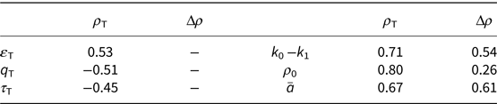
Although implicit equations might be expected to best represent the physical processes involved in the transition, more promising results are obtained by deriving simple, physically based, explicit expressions for ρ _T and Δρ. We begin with the concept that grain-boundary sliding can continue for longer if power-law creep is more difficult to initiate, that is, that the transition density should increase with the difference in densification rates, (k ₀ − k ₁). We further suppose that the particular combination of grain size and shape, grain bonding and layering that occurs at a given site, will also influence the transition parameters. We use ρ ₀, the surface intercept density, to discriminate between types of snow. Finally, as discussed in Section 2, we suppose that Δρ will have a threshold value set by the magnitude of the annual and sub-annual fluctuations in density and then increase with ā at higher accumulation rates. Table 2 shows higher r-values for these variables.

We select the two most significant variables, (k ₀ − k ₁) and ρ ₀, to derive an expression for the global value of the transition density, ρ _TG. Figure 12 shows the local values of ρ _T as a function of these variables against the background of the best linear fit to 29 evenly spaced points from the high-resolution groups, namely

(14)$$\eqalign{\rho_{\rm TG} & = \left[( 359 \pm400) \, \rm{kg}\, \rm{m}^{-3}\, \rm{m}\, \rm{w.e.}\right]\, \left(k_0 - k_1\right)\cr & \quad + \left[( 0.300 \, \pm \, 0.156) \right]\, \rho_0 \cr & \quad + \left[( 404\pm 51) \, \rm{kg}\, \rm{m}^{-3}\right]\quad r^2 = 0.72.}$$

The contours are shown at intervals of 10 kg m⁻³, the estimated uncertainty in individual points. The mean difference between global and local values is − 1 kg m⁻³. The r.m.s. of the differences is 12 kg m⁻³ for the high-resolution data and slightly greater, at 14 kg m⁻³, for Groups B and C, as we might expect. The extreme values of |ρ _TG − ρ _T| ≈ 30 kg m⁻³ come from Groups B and C. The points fall into two groups separated by ≈ 60 kg m⁻³ in ρ ₀ at the same value of (k ₀ − k ₁). In Section 4.2 we compared these groups to the H and L groups defined by Salamatin and others (Reference Salamatin2009), who suggested that different wind regimes produce different surface densities in otherwise similar climatic conditions. The corresponding difference in ρ _TG of ≈ 18 kg m⁻³ is comparable to the difference of (33 ± 8) kg m⁻³ in critical density values for H and L group profiles reported by Salamatin and Lipenkov (Reference Salamatin and Lipenkov2008).

Fig. 12.

Optimised values of the transition density ρ _T as a function of the difference in densification rates (k ₀ − k ₁) and the surface intercept density, ρ ₀. The contours are derived from a first-order polynomial fit to 29 selected values.

It has been suggested (Alley and Bentley, Reference Alley and Bentley1988; Riverman and others, Reference Riverman2017) that k ₁ may increase in areas of high strain rate. If this is so, we might expect a decrease in ρ _T with increasing $\dot {\epsilon }_{\rm H}$. Horizontal divergences for the iSTAR sites range up to a relatively high value of 8.9 × 10⁻³ a⁻¹ (Morris and others, Reference Morris2017) but we find no evidence of correlation between [ρ _T − ρ _TG] and $\dot {\epsilon }_{\rm H}$ for these data.

In Figure 13 the transition half-widths for the 73 selected profiles are shown, with their estimated errors, as a function of ā. The maximum likelihood estimate for Δρ of 45.5 kg m⁻³, shown in the figure, was calculated by fitting a Rayleigh distribution. This reflects the typical amplitude of density fluctuations observed in the high-resolution data. For $\bar {a} \gtrsim$ 0.6 m w.e. a⁻¹, Δρ increases with ā and there are ≈10 years in the transition zone. This suggests that decadal rather than annual variations in ρ′_T are controlling Δρ. For simplicity, we use the best fit expression

(15)$$\eqalign{\Delta\rho_G & = \left[( 79 \pm 25) \rm{m}\, \rm{w.e.}^{-1}\, \rm{a}\, {\rm kg}\, {\rm m}^{-3}\right]\, \bar{a} \cr & \quad + \left[( 32 \pm 10) \, \rm{kg}\, {\rm m}^{-3}\right]\quad r^2 = 0.36}$$

to estimate the global transition half-width, although this will slightly underestimate Δρ at very low-accumulation rates.

Fig. 13.

Optimised values of the transition half-width, Δρ, as a function of accumulation, ā. Error bars show the estimated uncertainty in individual values. The data are divided into groups according to the measurement techniques used and the quality of the density data (Section 3.3). The dashed lines show the maximum likelihood estimate for Δρ and the best linear fit. Labels show the estimated length of the transition zone in years.

We are now able to compare the performance of the HL(T) model using global parameters with the optimised HL(V) model. Figure 14 shows the difference between predicted and observed BCO heights for the 45 available profiles. The mean difference is now 0.64 m for the HL(T) model using global parameters, with an r.m.s. of 3.89 m, slightly greater than the value obtained using the local parameters but still 31% less than the value obtained using the HL model. The mean difference found using the HL(V) model is 0.84 m, with an r.m.s. difference of 5.20 m (a 7% improvement over the HL model). The HL(V) model produces a better fit than the transition model for the small ice cap profiles B38, B39 and Devon98 but a much worse fit for profiles such as South Pole and EDC2 with BCO depths >85 m. We should recall, however, that the HL(V) model parameters were derived using regional climate model inputs so are not necessarily the best possible set for the HL model using T _m and ā as inputs.

Fig. 14.

Difference between predicted and observed BCO heights. Predicted heights are calculated using the HL(V) model (Verjans and others, Reference Verjans2020) (◊), and the HL(T) model with global parameters ρ _TG and Δρ _G (♦). The points are divided into groups according to the measurement techniques used and the quality of the density data (Section 3.3).

Figure 15 shows the effect of making the thinning correction. For the 15 profiles corrected for thinning, the mean difference is 0.51 m for the HL(T) model with global parameters, − 1.39 m for the HL model and 0.82 m for the HL(V) model. The corresponding r.m.s. values are 2.82, 6.62 and 6.64 m. The improvement in r.m.s. of 58% for the transition model with respect to the HL(V) model is quite marked.

Fig. 15.

Difference between predicted and observed BCO heights, corrected for thinning. Predicted heights are calculated using the HL(V) model (Verjans and others, Reference Verjans2020) (◊), and the HL(T) model with global parameters ρ _TG and Δρ _G (♦). The points are divided into groups according to the measurement techniques used and the quality of the density data (Section 3.3).

It is important to remember that, since we match the observed and simulated profiles at the start of the transition region (see Section 2), the residual differences between modelled and observed nominal BCO depths are not affected by the choice of k ₀. They may indicate that the expression for k ₁ needs to be revised, but it is also the case that such differences could arise because of temporal variations in the climate or because the transition to stage 3 densification has begun before the nominal transition density of 815 kg m⁻³. Incorporating a gradual transition between stages 2 and 3 would be a natural extension of the HL(T) model.

6. Conclusion

We have adapted the classical Herron and Langway macroscale model for dry snow densification to include a transition zone between stage 1, in which grain-boundary sliding is the dominant process, and stage 2, in which power-law creep is dominant. In terms of the HL densification rates k ₀ and k ₁, the strain rate equation becomes

(16)$$\eqalign{\dot{\varepsilon} & = -{\bar{a}\over 2}\left({\rho_{\rm i}-\rho\over \rho}\right)\cr & \quad\times\left(\left(k_0 + k_1\right)-{2.06\left(k_0-k_1\right)\left({\rho-\rho_{\rm T} \over \Delta\rho}\right)\over \left\vert\left(1 + \left(2.06\left({\rho-\rho_{\rm T}\over \Delta\rho}\right)\right)^2\right)^{1/2}\right\vert}\right).}$$

We suggest equations for the transition parameters, ρ _T and Δρ, based on our view of the underlying physical processes:

(17)$$\eqalign{\rho_{\rm T} & = \left[( 359 \pm 400) \, \rm{kg}\, {\rm m}^{-3}\, \rm{m}\, {\rm w.e.}\right]\, \left(k_0 - k_1\right)\cr & \quad + \left[( 0.300 \pm 0.156) \right]\rho_0 + \left[( 404 \pm51) \, \rm{kg}\, {\rm m}^{-3}\right]}$$

and

(18)$$\eqalign{\Delta\rho & = \left[( 79 \, \pm \, 25) \, {\rm m\ w.e.}^{-1}\, {\rm a\ kg\ m}^{-3}\right]\, \bar{a} \cr & \quad + \left[( 32\, \pm \, 10) \, {\rm kg\ m}^{-3}\right],\; }$$

and show that predictions of the depth of the nominal BCO horizon, when the firn density reaches 815 kg m⁻³, are greatly improved by the inclusion of the transition zone. We have been limited by lack of high-resolution strain rate data which could be used to test the model directly; in order to use density profile data we have had to assume steady-state conditions with a constant accumulation rate. There is a clear need for more high-resolution field data, especially from the upper 20 m of the firn column, collected specifically to investigate the transition zone, rather than as a by-product of other studies. In the future, advances in methods for up-scaling from microscale snow physics to macroscale equations (e.g. Löwe and others, Reference Löwe, Riche and Schneebeli2013) will no doubt lead to improved equations for the transition parameters. For the moment we are content to make the point that incorporating a smooth transition into the benchmark dry snow densification model is a simple and effective way to improve its performance.

Supplementary materials

The supplementary material for this article can be found at https://doi.org/10.1017/jog.2021.95).

Acknowledgements

We acknowledge the many field researchers who have, over the years, collected the data without which this study would not have been possible. The SUMup database is supported by the U.S. National Science Foundation grant PLR 1603407. Pine Island Glacier data were collected as part of the iSTAR project funded by the UK Natural Environment Research Council under grant [10.13039/501100000270] (NE/J005797/1 and NE/J00569X/1). Skytrain data were collected as part of the WACSWAIN project funded by the European Research Council under Grant Agreement 742224. We thank Vincent Verjans and Yalalt Nyamgerel for interesting discussions and early sight of their data. We have been greatly helped by thoughtful reviews from Dr C Max Stevens and an anonymous reviewer and also thank our Scientific Editor, Dr Alan Rempel for his comments.

Appendix A. Density profile data

Table A1.

Optimised values for gamma-ray attenuation density profiles

Table A2.

Optimised values for neutron scattering density profiles

Table A3.

Optimised values for group A gravimetric density profiles

Table A4.

Optimised values for group B gravimetric density profiles

Table A5.

Optimised values for group C gravimetric density profiles

Footnotes

* Profile used to determine global equations for ρ _TG.

* Less than 10 measurements in transition zone.

References

Abram, NJ and 8 others (2013) Acceleration of snow melt in an Antarctic Peninsula ice core during the twentieth century. Nature Geoscience 6, 404–411. doi:10.1038/ngeo1787CrossRef Google Scholar

Alley, RB and Bentley, CR (1988) Ice-core analysis on the Siple Coast of West Antarctica. Annals of Glaciology 11, 1–7. doi:10.3189/S0260305500006236CrossRef Google Scholar

Arnaud, L, Lipenkov, VY, Barnola, JM, Gay, M and Duval, P (1998) Modelling of the densification of polar firn: characterization of the snow-firn transition. Annals of Glaciology 26, 39–44. doi:10.3189/1998aog26–1–39–44CrossRef Google Scholar

Arthern, RJ, Vaughan, DG, Rankin, AM, Mulvaney, R and Thomas, ER (2010) In-situ measurements of Antarctic snow compaction compared with predictions of models. Journal of Geophysical Research 115(F03011) 10.1029/2009JF001306.CrossRef Google Scholar

Bader, HP and Weilenmann, P (1992) Modeling temperature distribution, energy and mass flow in a (phase-changing) snowpack. i. model and case studies. Cold Regions Science and Technology 20, 157–181.CrossRef Google Scholar

Barnola, JM, Pimienta, P, Raynaud, D and Korotkevich, YS (1991) CO₂-climate relationship as deduced from the Vostok ice core – a re-examination based on new measurements and on a re-evaluation of the air dating. Tellus B 43(2), 83–90. doi:10.1034/j.1600–0889.1991.t01–1–00002.xCrossRef Google Scholar

Benson, CS (1962) Stratigraphic studies in the snow and firn of the Greenland Ice Sheet. SIPRE Research Report 70, 93. doi:10.21236/ada337542Google Scholar

Breton, DJ, Hamiliton, GS and Hess, CT (2009) Instruments and methods design, optimization and calibration of an automated density gauge for firn and ice cores. Journal of Glaciology 55(194), 1092–1100. doi:10.3189/002214309790794841CrossRef Google Scholar

Brun, E, Martin, E, Simon, V, Gendre, C and Coleov, C (1989) An energy and mass model of snow cover suitable for operational avalanche forecasting. Journal of Glaciology 35(121), 333–342. (doi:10.3189/S0022143000009254)CrossRef Google Scholar

Ebinuma, T and Maeno, N (1987) Particle rearrangement and dislocation creep in a snow-densification process. Journal de Physique Colloque 3(48 Suppl.), 263–269. doi:10.1051/jphyscol:1987137Google Scholar

Fourteau, K, Gillet-Chaulet, F, Martinerie, P and Fan, X (2020) A micro-mechanical model for the transformation of dry polar firn into ice using the level-set method. Frontiers in Earth Science 8(101). doi:10.3389/feart.2020.00101).CrossRef Google Scholar

Freitag, J, Wilhelms, F and Kipfstuhl, S (2004) Microstructure-dependent densification of polar firn derived from x-ray microtomography. Journal of Glaciology 50(169), 243–250. doi:10.3189/172756504781830123CrossRef Google Scholar

Gerland, S and 5 others (1999) Density log of a 181 m long ice core from Berkner Island, Antarctica. Annals of Glaciology 29, 215–219. doi:10.3189/172756499781821427CrossRef Google Scholar

Goujon, C, Barnola, JM and Ritz, C (2003) Modeling the densification of polar firn including heat diffusion: application to close-off characteristics and gas isotopic fractionation for Antarctica and Greenland sites. Journal of Geophysical Research 108(D24)doi:10.1029/2002JD003319.CrossRef Google Scholar

Hawley, RL and Morris, EM (2006) Borehole optical stratigraphy and neutron-scattering density measurements at Summit, Greenland. Journal of Glaciology 52(179), 491–496. doi:10.3189/172756506781828368CrossRef Google Scholar

Hawley, RL, Morris, EM and McConnell, JR (2008) Rapid techniques for determining annual accumulation applied at Summit, Greenland. Journal of Glaciology 54(188), 839–845. doi:10.3189/002214308787779951CrossRef Google Scholar

Herron, MM and Langway, CC (1980) Firn densification: an empirical model. Journal of Glaciology 25(93), 373–385. doi:10.3189/S002214300001523CrossRef Google Scholar

Hörhold, MW, Kipfstuhl, S, Wilhelms, F, Freitag, J and Frenzel, A (2011) The densification of layered polar firn. Journal of Geophysical Research: Earth Surface 116(F1), 1–15. doi:10.1029/2009jf001630CrossRef Google Scholar

Hörhold, MW and 5 others (2012) On the impact of impurities on the densification of polar firn. Earth and Planetary Science Letters 325–326, 93–99. doi:10.1016/j.epsl.2011.12.022CrossRef Google Scholar

Horlings, AN, Christianson, K, Holschuh, ND, Stevens, CM and Waddington, ED (2020) Effect of horizontal divergence on estimates of firn-air content. Journal of Glaciology 67(262), 287–296. doi:10.1017/jog.2020.105CrossRef Google Scholar

Jordan, R (1991) A one-dimensional temperature model for a snow cover. Technical documentation for SNTHERM.89. Cold Regions Research and Engineering Laboratory Special Report, 657.Google Scholar

Kameda, T, Shoji, H, Kawada, K, Watanabe, O and Clausen, HB (1994) An empirical relation between overburden pressure and firn density. Annals of Glaciology 20, 87–94. doi:10.3189/1994aog20–1–87–94Google Scholar

Koerner, RM (1977) Devon Island Ice Cap: Core stratigraphy and paleoclimate. Science (New York, N.Y.) 196(4285), 15–18. doi:10.1126/science.196.4285.15CrossRef Google Scholar PubMed

Ligtenberg, SRM, Helsen, MM and van den Broeke, MR (2011) An improved semi-empirical model for the densification of Antarctic firn. The Cryosphere 5(4), 809–819. doi:10.5194/tc–5–809–2011CrossRef Google Scholar

Löwe, H, Riche, F and Schneebeli, M (2013) A general treatment of snow microstructure exemplified by an improved relation for the thermal conductivity. The Cryosphere 7, 1743. doi:10.5194/tc–7–1473–2013CrossRef Google Scholar

Lundin, J and 12 others (2017) Firn model intercomparison experiment (FirnMICE). Journal of Glaciology 63(239), 401–422. (doi:10.1017/jog.2016.114)CrossRef Google Scholar

Martinerie, P and 5 others (1994) Air content paleo record in the Vostok ice core (Antarctica): a mixed record of climatic and glaciological parameters. Journal of Geophysical Research 99(D5), 10565–10576. doi:10.1029/93JD03223CrossRef Google Scholar

Montgomery, LN, Koenig, L and Alexander, P (2018) The SUMup dataset: compiled measurements of surface mass balance components over ice sheets and sea ice with preliminary analysis over Greenland. Earth System Science Data 10(4), 1959–1985. doi:10.5194/essd–10–1959–2018CrossRef Google Scholar

Morris, EM and 9 others (2017) Snow densification and recent accumulation along the iSTAR Traverse, Pine Island Glacier, Antarctica. Journal of Geophysical Research: Earth Surface 122, 2284–2301. doi:10.1002/2017jf004357CrossRef Google Scholar

Morris, EM (2018) Modelling dry-snow densification without abrupt transition. Geosciences 8(12), 464. doi:10.3390/geosciences8120464CrossRef Google Scholar

Morris, EM and Cooper, JD (2003) Density measurements in ice boreholes using neutron scattering. Journal of Glaciology 49(167), 599–604. doi:10.3189/17275650378183040CrossRef Google Scholar

Morris, EM and Wingham, DJ (2014) Densification of polar snow: measurements, modelling and implications for altimetry. JGR Earth Surfaces 119. doi:10.1002/2013JF002898Google Scholar

Nye, JF (1963) Correction factor for accumulation measured by the thickness of annual layers in an ice sheet. Journal of Glaciology 4(36), 785–788. doi:10.3189/S0022143000028367CrossRef Google Scholar

Parrenin, F and 15 others (2007) 1-D-ice flow modelling at EPICA Dome C and Dome Fuji, East Antarctica. Climate of the Past 3(2), 243–259. doi:10.5194/cp–3–243–2007CrossRef Google Scholar

Paterson, WSB and Waddington, E (1984) Past precipitation rates derived from ice core measurements: methods and data analysis. Reviews of Geophysics and Space Physics 22(2), 123–130. doi:10.1029/rg022i002p00123CrossRef Google Scholar

Raymond, C and 5 others (1996) Geometry, motion and mass balance of Dyer Plateau, Antarctica. Journal of Glaciology 42, 510–518. doi:10.3189/s002214300000349xCrossRef Google Scholar

Reeh, N, Fisher, DA, Koerner, RM and Clausen, HB (2005) An empirical firn-densification model comprising ice lenses. Annals of Glaciology 42, 101–106. doi:10.3189/172756405781812871CrossRef Google Scholar

Riverman, K and 7 others (2017) Enhanced firn densification in high accumulation shear margins of the NE Greenland Ice Stream. Journal of Geophysical Research Earth Surface 124, 365–382. doi:10.1029/2017JF004604CrossRef Google Scholar

Salamatin, AN and Lipenkov, VY (2008) Simple relations for the close-off depth and age in dry-snow densification. Annals of Glaciology 49, 71–76. doi:10.3189/172756408787814889CrossRef Google Scholar

Salamatin, AN and 5 others (2009) Snow/firn densification in polar ice sheets. In T Hondoh (ed.), Physics of Ice Core Records II, volume 68 of Low Temperature Science, 195–222, ILTS, Hokkaido University, Sapporo.Google Scholar

Schmidt, KM and 5 others (2014) Calcium, dust and nitrate concentrations in monthly resolution in ice core DML94C07_38 (B38). PANGAEA 4. doi:10.1594/PANGAEA.837875Google Scholar

Simonsen, SB and 5 others (2013) Assessing a multilayered dynamic firn-compaction model for Greenland with ASIRAS radar measurements. Journal of Glaciology 59(215), 545–558. doi:10.3189/2013jog12j158CrossRef Google Scholar

Spencer, M, Alley, RB and Creyts, T (2001) Preliminary firn-densification model with 38-site dataset. Journal of Glaciology 47(159), 671–676. doi:10.3189/172756501781831765CrossRef Google Scholar

Verjans, V and 6 others (2020) Bayesian calibration of firn densification models. The Cryosphere 13, 3023–3043. doi:10.5194/tc–2019–274Google Scholar

Wilhelms, F (1996) Leitfähigkeits- und Dichtemessungen an Eisbohrkernen (Measuring the conductivity and density of ice cores). Berichte zur Polarforschung 191, 224.Google Scholar

Fig. 1. Distribution of density profiles used in this study with mean annual temperature, Tm, and mean annual accumulation, ā. The profiles are divided into groups according to the measurement techniques used (gamma-ray attenuation (γ), neutron scattering (np) and gravimetric (grav.)) and the quality of the data (A, B, C). Above the dashed line the Herron and Langway (1980) stage 1 densification rate is greater than the stage 2 rate.

Fig. 2. Observed and modelled profiles of R = ln(ρ/(ρi − ρ)) for core B36/B37. The very high-resolution density data Robs were collected using a gamma-ray attenuation technique. Horizontal dotted lines show the extent of the transition region from stage 1 to stage 2 densification, that is, ρT ± Δρ, and the nominal transition to stage 3. The extended HL stage 1 and 2 curves cross at 550 kg m−3. The parameters of the transition model HL(T) are optimised to produce the best fit to Rs, which is a polynomial fit to the observed data across the transition region.

Fig. 3. Observed and modelled profiles of R = ln(ρ/(ρi − ρ)) for site B38. The very high-resolution density data Robs were collected using a gamma-ray attenuation technique. Horizontal dotted lines show the extent of the transition region from stage 1 to stage 2 densification, that is, ρT ± Δρ, and the nominal transition to stage 3. The extended HL stage 1 and 2 curves cross at 550 kg m−3. The parameters of the transition model HL(T) are optimised to produce the best fit to Rs, which is a polynomial fit to the observed data across the transition region.

Fig. 4. Best value of ρT from neutron scattering density profiles at 10 iSTAR sites as a function of the best value from gravimetric profiles nearby. The solid line shows a 1:1 relationship and dotted lines indicate an uncertainty of ± 10 kg m−3.

Fig. 5. Best value of Δρ from neutron scattering density profiles at 10 iSTAR sites as a function of the best value from gravimetric profiles nearby. The solid line shows a 1:1 relationship and dotted lines indicate an uncertainty of ± 40 kg m−3.

Fig. 6. Best value of ρ0 from neutron scattering density profiles at 10 iSTAR sites as a function of the best value from gravimetric profiles nearby. The solid line shows a 1:1 relationship and dotted lines indicate an uncertainty of ± 7 kg m−3.

Table 1. Optimised parameters for profile pairs

Fig. 7. Variation of surface intercept density, ρ0, with (a) mean annual temperature, Tm, and (b) mean annual accumulation, ā, for the density profiles used in this study. The data are divided into groups according to the measurement techniques used and the quality of the density data (Section 3.3).

Fig. 8. Optimised values of the transition density, ρT, for individual profiles as a function of mean annual temperature, Tm, mean annual accumulation, ā and the surface intercept density, ρ0.

Fig. 9. Optimised values of the transition half-width, Δρ, for individual profiles as a function of mean annual temperature, Tm, mean annual accumulation, ā and the surface intercept density, ρ0.

Fig. 10. Difference between predicted and observed BCO heights. Predicted heights are calculated using the HL model (◊), and the HL(T) model with local optimised values of ρT and Δρ (♦). The points are divided into groups according to the measurement techniques used and the quality of the density data (Section 3.3).

Fig. 11. Difference between predicted and observed BCO heights, corrected for thinning. Predicted heights are calculated using the HL model (◊), and the HL(T) model with local best values of ρT and Δρ (♦). The points are divided into groups according to the measurement techniques used and the quality of the density data (Section 3.3).

Table 2. Pearson's r for 73 profiles

Fig. 12. Optimised values of the transition density ρT as a function of the difference in densification rates (k0 − k1) and the surface intercept density, ρ0. The contours are derived from a first-order polynomial fit to 29 selected values.

Fig. 13. Optimised values of the transition half-width, Δρ, as a function of accumulation, ā. Error bars show the estimated uncertainty in individual values. The data are divided into groups according to the measurement techniques used and the quality of the density data (Section 3.3). The dashed lines show the maximum likelihood estimate for Δρ and the best linear fit. Labels show the estimated length of the transition zone in years.

Fig. 14. Difference between predicted and observed BCO heights. Predicted heights are calculated using the HL(V) model (Verjans and others, 2020) (◊), and the HL(T) model with global parameters ρTG and ΔρG (♦). The points are divided into groups according to the measurement techniques used and the quality of the density data (Section 3.3).

Fig. 15. Difference between predicted and observed BCO heights, corrected for thinning. Predicted heights are calculated using the HL(V) model (Verjans and others, 2020) (◊), and the HL(T) model with global parameters ρTG and ΔρG (♦). The points are divided into groups according to the measurement techniques used and the quality of the density data (Section 3.3).

Table A1. Optimised values for gamma-ray attenuation density profiles

Table A2. Optimised values for neutron scattering density profiles

Table A3. Optimised values for group A gravimetric density profiles

Table A4. Optimised values for group B gravimetric density profiles

Table A5. Optimised values for group C gravimetric density profiles

Morris et al. supplementary material

PDF 262.5 KB

Article contents

Modelling the transition from grain-boundary sliding to power-law creep in dry snow densification

Abstract

Keywords

Information

List of symbols

1. Introduction

2. The transition model

3. Data

3.1. Profiles used in this study

3.2. Excluded profiles

3.3. Climatic distribution of the data

4. Results

4.1. Estimation of the uncertainty in model parameters

4.2. Surface intercept density

4.3. The transition density

4.4. The transition range

5. Discussion

5.1. Physical interpretation of the transition parameters

5.2. Densification parameters

5.3. Prediction of the BCO horizon

5.4. Prediction of DIP

5.5. Derivation of global parameters

6. Conclusion

Supplementary materials

Acknowledgements

Appendix A. Density profile data

Footnotes

References

Morris et al. supplementary material

Save article to Kindle

Save article to Dropbox

Save article to Google Drive

Reply to: Submit a response

Your details

You have entered the maximum number of contributors

Conflicting interests