


1. Introduction
Clusters of galaxies are among the largest structures in the Universe. Understanding how clusters form and their dynamics is key to understanding how the Universe behaves on some of the largest scales. Galaxy clusters are thought to form in the hierarchical model, where galaxies eventually clump together during sometimes intense merger events (Peebles Reference Peebles1980). The clusters themselves are primarily dark matter, diffuse gas that makes up the intra-cluster medium (ICM), and the galaxies for which they are named. Galaxy clusters are found to host magnetic fields on the order of 0.1–1  $\upmu$G (Clarke, Kronberg, & Böhringer 2001; Johnston-Hollitt Reference Johnston-Hollitt2003; Bonafede et al. Reference Bonafede, Feretti, Murgia, Govoni, Giovannini, Dallacasa, Dolag and Taylor2010). The magnetic fields in clusters give rise to radio synchrotron emission; relativistic electrons accelerated by the magnetic fields with Lorentz factors of $\gamma > 1\,000$, where the spectral energy distribution (SED) of the emission gives insight into the ages of electron populations and the possible shock-driven reacceleration from merger events (see Feretti et al. Reference Feretti, Giovannini, Govoni and Murgia2012; Brunetti & Jones Reference Brunetti and Jones2014; van Weeren et al. Reference van Weeren, de Gasperin, Akamatsu, Brüggen, Feretti, Kang, Stroe and Zandanel2019, for reviews). The steep spectral indicesFootnote a of such synchrotron emission means that to detect the faintest non-thermal diffuse cluster emission low-frequency radio telescopes are required, such as the Giant Metrewave Radio Telescope (GMRT; Ananthakrishnan Reference Ananthakrishnan1995), the Murchison Widefield Array (MWA; Tingay et al. Reference Tingay2013), and the LOw Frequency ARray (LOFAR; van Haarlem et al. Reference van Haarlem2013). As radio telescopes become more sensitive, more of this steep-spectrum diffuse emission is expected to be found (Cassano et al. Reference Cassano, Brunetti, Norris, Rottgering, Johnston-Hollitt and Trasatti2012; Johnston-Hollitt Reference Johnston-Hollitt2017).
Diffuse synchrotron emission comes in two main classes: cluster haloes and relics. Cluster relics can be broken down further into two types: kpc-scale phoenices and megaparsec-scale relics. The kpc-scale radio phoenices are thought to be emission from revived fossil plasma left over from long dormant radio galaxies (see, e.g. Enßlin & Gopal-Krishna 2001; Enßlin & Brüggen 2002) and are usually found near the cluster centre (e.g. Slee et al. Reference Slee, Roy, Murgia, Andernach and Ehle2001). Megaparsec-scale relics (hereafter relics) are thought to trace shocks through the ICM during and after massive merger events. These are found on the periphery of clusters, usually aligned with the major merger axis and can come in adjacent pairs of so-called double relics (e.g. Abell 3667; Johnston-Hollitt Reference Johnston-Hollitt2003, Abell 3376; Bagchi et al. Reference Bagchi, Durret, Neto and Paul2006, PSZ1 G108.18–11.53; de Gasperin et al. Reference de Gasperin, Intema, van Weeren, Dawson, Golovich, Wittman, Bonafede and Brüggen2015). For both types of relics, the electrons must go through some reacceleration process albeit on vastly different scales. These processes are thought to be through shocks typically resulting in an elongated or arc-like morphology in the case of relics. The key observed distinction between the two types of emission are their size and spectral properties. Phoenices, thought to form through adiabatic shock compression, can show curved spectra (Enßlin & Gopal-Krishna 2001), whereas relic spectra typically resemble power laws (e.g. Hindson et al. Reference Hindson2014; George et al. Reference George2017; Rajpurohit et al. Reference Rajpurohit2020).
Haloes also come in two main types: mini-haloes and cluster haloes. Mini-haloes are associated with strong active galactic nuclei (AGN), often the central dominant (cD) galaxy within the core of the cluster, and are smaller in extent though are otherwise morphologically similar to cluster haloes (for a recent review, see Bravi, Gitti, & Brunetti Reference Bravi, Gitti and Brunetti2016). Cluster haloes are centrally located within the cluster, morphologically regular, and are often found to coincide with the X-ray emitting plasma of the ICM. Haloes do not normally show any significant fractional polarisation, however, this is likely a limitation of the resolution of current-generation radio interferometers (Govoni et al. Reference Govoni, Murgia, Xu, Li, Norman, Feretti, Giovannini and Vacca2013). The mechanism that generates these radio haloes is still under investigation. The primary, reacceleration model of halo generation suggests the synchrotron emission occurs after electrons are reaccelerated through merger-driven turbulence in the magnetised ICM (see e.g. Brunetti et al. Reference Brunetti, Setti, Feretti and Giovannini2001; Buote Reference Buote2001; Petrosian Reference Petrosian2001; Petrosian & East Reference Petrosian and East2008; Cassano et al. Reference Cassano, Brunetti, Norris, Rottgering, Johnston-Hollitt and Trasatti2012). An alternate model is that of hadronic origin (see e.g. Dennison Reference Dennison1980; Dolag & Enßlin 2000). In this secondary model, electrons are generated as secondary products of collisions between cosmic ray protons and ICM protons. Pions, a product in these proton–proton collisions, produce the electrons that will be accelerated by magnetic fields, as well as  $\gamma$-rays. This model not only requires $\gamma$-ray emission from clusters but also that all galaxy clusters host radio haloes at some level. The synchrotron emission from electrons produced through these proton-proton collisions will be significantly weaker than that seen through reacceleration via turbulence (Blasi & Colafrancesco Reference Blasi and Colafrancesco1999). So far, only upper limits for $\gamma$-ray emission have been presented (e.g. Ackermann et al. Reference Ackermann2014; Prokhorov & Churazov Reference Prokhorov and Churazov2014; Liang et al. Reference Liang2016), and with current generation radio telescopes, the necessary sensitivity to detect haloes generated through the secondary model alone has not been reached. The primary and secondary models are not mutually exclusive, and there has been work to combine the two models (e.g. Brunetti & Blasi Reference Brunetti and Blasi2005; Brunetti & Lazarian Reference Brunetti and Lazarian2011, Reference Brunetti and Lazarian2016). The primary model is observationally supported by the fact that predominantly unrelaxed, X-ray luminous clusters are known to host radio haloes. However, radio halo detection had been biased towards those clusters hosting highly X-ray luminous plasma as these are the clusters often targeted (e.g. Giovannini, Tordi, & Feretti Reference Giovannini, Tordi and Feretti1999; Venturi et al. Reference Venturi, Giacintucci, Brunetti, Cassano, Bardelli, Dallacasa and Setti2007; Venturi et al. Reference Venturi, Giacintucci, Dallacasa, Cassano, Brunetti, Bardelli and Setti2008; Kale et al. Reference Kale, Venturi, Giacintucci, Dallacasa, Cassano, Brunetti, Macario and Athreya2013, Reference Kale2015). Only recently have surveys been conducted to search for diffuse cluster emission without preselecting clusters based solely on their X-ray luminosities. For example, Bernardi et al. (Reference Bernardi2016) select clusters based on mass, and Shakouri et al. (Reference Shakouri, Johnston-Hollitt and Pratt2016) survey clusters over a wide range of X-ray luminosities.
Given the comparative rarity of diffuse cluster emission detection, we wish to perform larger surveys to properly ascertain the incidence and nature of these types of radio emission. In this paper, we present the results of one such survey using a deep  $45^{\circ} \times 45^{\circ}$ image produced by the MWA as part of the MWA Epoch of Reionization (EoR) project (Bowman et al. Reference Bowman2013; Offringa et al. Reference Offringa2016). This study forms the pilot for a larger search for diffuse cluster emission (Johnston-Hollitt et al. in preparation) using the recently released GaLactic and Extragalactic All-sky MWA survey (GLEAM; Wayth et al. Reference Wayth2015), which covers the entire southern sky below a declination of $+25^{\circ}$ and covers the frequency range 72–231 MHz. In the following sections, we discuss the various images used and the process involved in searching for diffuse cluster emission.
This paper unless otherwise stated assumes a flat  $\Lambda$CDM cosmology with $H_0 = 70\,\textrm{km\,s}^{-1}\,\textrm{Mpc}^{-1}$, $\Omega_\textrm{M} = 0.3$, and $\Omega_\Lambda = 1-\Omega_\textrm{M}$.
2. The search for diffuse cluster emission
2.1. The Epoch of Reionization 0-h field
As part of the MWA EoR project, Offringa et al. (Reference Offringa2016) present a  $45^{\circ} \times 45 ^{\circ}$ image centred on $(\alpha_{\textrm{J2000}},\,\delta_{\textrm{J2000}}) = (00^{\textrm{h}}00^{\textrm{m}}00^{\textrm{s}}, -27^{\circ}00\ensuremath{'}00\ensuremath{''})$, at a frequency of 168 MHz called the EoR0 field. This image is obtained from 45 h of integration and has a resolution of 2.3 arcmin. The EoR0 field is the deepest, confusion limited image made with the 128-tile Phase I MWA.Footnote b In addition to the overall sensitivity, the low surface brightness imaging capability provided by the number of short ( $\leq 60\,\textrm{m}$) baselines makes the MWA a powerful tool to investigate extended, diffuse emission. Data collection, reduction, and imaging for the field used here are explained in detail in Offringa et al. (Reference Offringa2016). Whilst the primary purpose of the EoR0 field is the study of EoR, the image itself is incredibly sensitive for an MWA image at this frequency, reaching down to $\sim$2.3 $\text{mJy}\,\text{beam}^{-1}$ near the centre of the image and increasing up to $\sim$100 $\text{mJy}\,\text{beam}^{-1}$ out towards the image edges. This surface brightness sensitivity makes the EoR0 field useful in the search for steep spectrum cluster haloes and relics. The R.A. and decl. range used here is as follows: $(22^{\textrm{h}}29^{\textrm{m}}55{^{\textrm s}}.2 \leq \alpha_{\textrm{J2000}} \leq 01^{\textrm{h}}29^{\textrm{m}}57{^{\textrm s}}.6)$ and $(\!-44^{\circ}41\ensuremath{'}24\ensuremath{''} \leq \delta_{\textrm{J2000}} \leq -08^{\circ}36\ensuremath{'}36\ensuremath{''})$, which is chosen to cut out the most significant noise at the edge of the image.
2.2. Catalogues of galaxy clusters
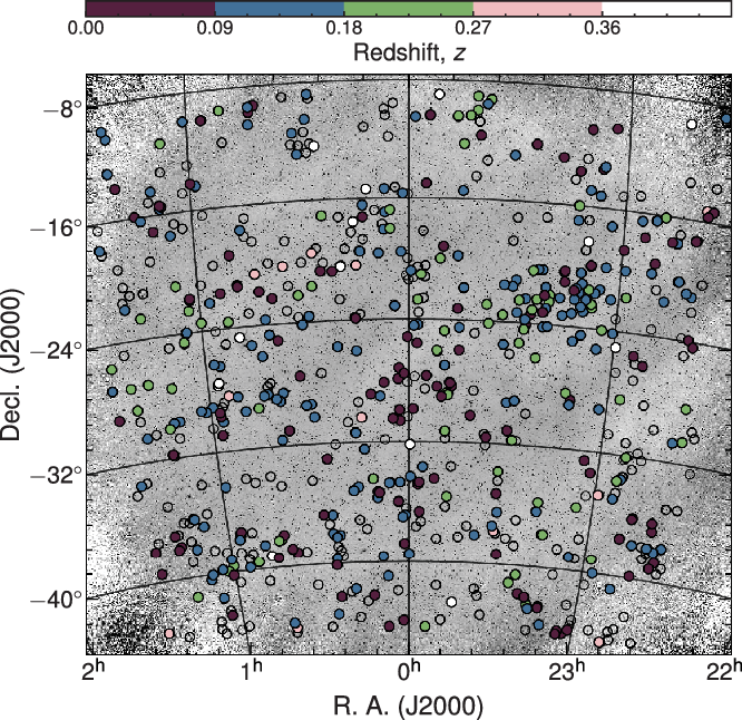
Within the EoR0 field we searched for diffuse emission within a  $\sim$2 Mpc radius around clusters within the following catalogues: Abell revised North, South, and Supplementary catalogues (Abell et al. Reference Abell1989, hereafter ACO, but see also Abell Reference Abell1958); the Meta-Catalogue of X-ray detected Clusters of galaxies (Piffaretti et al. Reference Piffaretti, Arnaud, Pratt, Pointecouteau and Melin2011, hereafter MCXC); the Planck catalogue of Sunyaev–Zel’dovich sources (Planck Collaboration et al. 2015, hereafter PSZ1).Footnote c Within the region encompassed by the EoR0 field, and excluding those clusters that lie too far to the edge of the image, this constitutes 668 unique clusters, 505 unique to ACO, 70 unique to MCXC, and 19 unique to PSZ1, with 24 clusters present in all three catalogues. Figure 1 shows the distribution of ACO, PSZ1, and MCXC clusters within the EoR0 field, coloured by redshift where available.
The central  $\sim42^{\circ}$ of the Epoch of Reoinization 0-h field. Overlaid are the positions of galaxy clusters from the (Abell, Corwin, & Olowin 1989) catalogues, Reference Piffaretti, Arnaud, Pratt, Pointecouteau and MelinMCXC and the PSZ1. We cut the sample of clusters in an attempt to avoid the edges of the image where the noise is highest. The filled circles are coloured according to their redshift. Unfilled circles are those without a measured redshift. Note the side-lobe structure of the primary beam appearing in the corners of the image. The colourmap of the redshift distribution is an implementation of cubehelix (Green Reference Green2011).
All clusters are checked systematically for diffuse cluster emission except 217 clusters in the ACO catalogue without a redshift. For clusters without a redshift, we are unable to determine the projected linear distance from the cluster centre, which makes determining if emission is part of the cluster difficult if not at the centre. Whilst this does not pose much problem for haloes, we also consider that ACO clusters without a redshift are unlikely to have auxiliary data in the form of cluster mass, X-ray luminosities, or information on cluster members. Further, cluster emission serendipitously found in clusters not part of the aforementioned catalogues is investigated when noticed.
2.3. Source detection and measurement
2.3.1. Manual source finding: eyeballing galaxy clusters
While source-finding algorithms exist and are put to good use to produce point-source catalogues, automated source-finding can miss the extended, low surface brightness haloes, and relics within clusters (Hollitt & Johnston-Hollitt Reference Hollitt and Johnston-Hollitt2012). Therefore, the EoR0 field is searched by eye for diffuse emission. Auxiliary radio data exist in the form of the following sky surveys: the NRAO VLA Sky SurveyFootnote d (NVSS; Condon et al. Reference Condon, Cotton, Greisen, Yin, Perley, Taylor and Broderick1998), the Sydney University Molonglo Sky Survey (SUMSS; Bock, Large, & Sadler Reference Bock, Large and Sadler1999; Mauch et al. Reference Mauch, Murphy, Buttery, Curran, Hunstead, Piestrzynski, Robertson and Sadler2003), the TFIRFootnote e GMRT Sky Survey (alternate data release, TGSS; Intema et al. Reference Intema, Jagannathan, Mooley and Frail2017), and the VLA Low-frequency Sky Survey redux (VLSSr; Lane et al. Reference Lane, Cotton, van Velzen, Clarke, Kassim, Helmboldt, Lazio and Cohen2014). These surveys and their salient properties are summarised in Table 1. Beyond radio surveys, we use the RÖentgen SATellite (ROSAT; Trümper Reference TrÜmper1984), All-Sky Survey (RASS; Voges et al. Reference Voges1999), the Digitized Sky Survey (DSS2), the first Pan-STARRSFootnote f survey— PS1 (Tonry et al. Reference Tonry2012; Chambers et al. Reference Chambers2016), the Dark Energy Survey Data Release 1 (DES DR1; Abbott et al. Reference Abbott2018; Morganson et al. Reference Morganson2018; Flaugher et al. Reference Flaugher2015), as well as archival Chandra data with the Advanced CCD Imaging Spectrometer (ACIS) instrument and XMM-Newton data with the European Photon Imaging Camera (EPIC) instrument, where available. For a small selection of clusters, we utilise deep ( ${>}30\,\textrm{ks}$ exposure) X-ray images from the Representative XMM-Newton Cluster Structure Survey (REXCESS; Böhringer et al. 2007; Pratt et al. Reference Pratt, Croston and Arnaud2009).
Existing sky surveys used as auxiliary data to the EoR0 field.

a At  $\delta_{\text{J2000}} = -27^{\circ}$.
To determine the nature of detected emission, we look for the following:
i. high-frequency counterparts (1.4 GHz and 843 MHz),
ii. low-frequency counterparts (147.5 and 74 MHz),
iii. optical identifications, and
iv. X-ray emission coincident with centrally located radio emission.
(i) and (ii) are used as an easy method of checking if we are looking at blended point sources; (i) gives a quick insight into the spectral index of the source, with significant high-frequency emission, at least comparably to 168 MHz, a flat spectral index is present which is uncharacteristic of diffuse cluster emission; (iii) is important as cluster haloes and relics are not associated with an optically visible galaxy, though in the case of cluster haloes there is expected to be a concentration of optically visible galaxies due to the central location in the cluster. If an optically visible galaxy is found at the peak of the diffuse emission or between two lobes, then the likelihood is that of extended, disturbed, or otherwise normal lobes of a radio galaxy; and (iv) allows us to confidently classify centrally located diffuse emission as a cluster halo or relic. In particular, Chandra or XMM-Newton observations are detailed enough to provide the position and any elongation of the X-ray emission relative to any centrally located diffuse radio emission. With these points forming the foundations of our search, we eyeballed the subset of clusters described in Section 2.2, followed by measurements of relevant physical properties.
2.3.2. Local noise properties
The EoR0 field is a large image that has greatly varying rms noise throughout. However, corners of the image feature significant noise due to the primary beam null. Offringa et al. (Reference Offringa2016) use the Background And Noise Estimation (BANE) toolFootnote g (Hancock et al. Reference Hancock, Murphy, Gaensler, Hopkins and Curran2012) to estimate noise throughout the EoR0 field. The mean noise level is calculated to be  $3.2 \pm 0.6$ $\text{mJy}\,\text{beam}^{-1}$ for the central $10^\circ$ of the image. Large-scale diffuse structure of Galactic origin is seen streaking the image which leads to non-constant background signal affecting rms noise calculations. In regions with no Galactic emission, the rms can be as low as $\sim$2 $\text{mJy}\,\text{beam}^{-1}$. Additionally, typical local rms noise values for the various survey data are provided in Table 1.
2.3.3. Integrated flux densities
The software that generated the EoR0 field at the time did not calculate a correct synthesized beam for the restored, stacked image. As a result, the integrated flux densities measured directly from the image are incorrect. We find that the integrated flux density measurements of the EoR0 field differed by a systematic factor of approximately 30% when compared to the nearly equivalent 162–170 MHz band in the GLEAM survey which is tied to the Baars flux scale (Baars et al. Reference Baars, Genzel, Pauliny-Toth and Witzel1977).
To scale the integrated flux densities in the EoR0 field, we choose six reasonably bright ( $>2\,\textrm{Jy}$) unresolved sources, exhibiting no side-lobe structure and no blending with nearby sources. From a linear fit between the GLEAM 162–170 MHz and EoR0 168 MHz flux densities, we find a factor $0.69 \pm 0.05$ to be used for calibration of measured integrated flux densities (i.e., $S_{168,\textrm{corrected}} = 0.69 \times S_{168}$), and this calibration is used through the remainder of this paper.
Flux densities of extended sources are either calculated by purpose-built fluxtools.pyFootnote h code or by using aegean if sources are blended, as the aforementioned python code does not fit sources, and assumes each source is discrete. Both methods measure the source flux densities down to the 2.6 $\sigma_{\textrm{rms}}$ level so as to include as much real contribution from the faint sources as possible (e.g. Kapińska et al. 2017, but see also Hales et al. Reference Hales, Murphy, Curran, Middelberg, Gaensler and Norris2012). We do not use aegean for all sources as aegean is intended as a point-source finder and will give the best results measuring such sources. Each flux measurement has an uncertainty, $\sigma_{S_\nu}$, calculated as
 \begin{equation}\sigma_{S_\nu} = \sqrt{ {S_\nu}^2 \left({\sigma_\textrm{scale}}^2 + {\sigma_\textrm{rescale}}^2 \right) + \left( \sigma_{\textrm{rms}} \sqrt{N_{\textrm{beam}}} \right)^2} \quad [\textrm{Jy}] \, ,\end{equation}
where  $N_{\textrm{beam}}$ is the number of beams crossing the extended source, $\sigma_\textrm{scale} = 5\%$—the flux scale error as described in Section 4.1 of Offringa et al. (Reference Offringa2016), and $\sigma_\textrm{rescale} = 5\%$ for the additional uncertainty in rescaling the integrated flux density measurements. The last term is the standard error given to flux density measurements of extended sources.
2.3.4. Spectral indices and source sizes
Where possible a spectral index is calculated for each source assuming the SED follows a standard power law in the relevant frequency range. This is either done as a two-point spectral index ( $\alpha = \ln\left(S_1 / S_2 \right) / \ln\left(\nu_1 / \nu_2 \right)$) or by fitting a first-order polynomial to the flux density measurements in log–log space, hence fitting a power law to the data. Over the frequency range here (74–1 400 MHz) haloes and relics tend not to show any turnovers or breaks and typically do not deviate from the assumed power law except in rare instances (e.g. the relic in Abell 2443 which has a break near 325 MHz reported by Cohen & Clarke Reference Cohen and Clarke2011). Phoenices, however, can show curved spectra (e.g. Slee et al. Reference Slee, Roy, Murgia, Andernach and Ehle2001; Kale & Dwarakanath Reference Kale and Dwarakanath2012). For the purpose of this work (and often in the absence of more than two flux density measurements), we assume power laws model these SEDs sufficiently in the relevant frequency regime as is often the case (see e.g. Abell 0013; George et al. Reference George2017).
Where appropriate, we estimate limits to flux densities. In particular, we use this for estimating 1.4 and 147.5 MHz limits when 168 MHz emission has no counterpart in the NVSS or TGSS survey images, respectively. These are used then to impose limits on the spectral indices. For such sources, we estimate the source area at 168 MHz, which is a function of the MWA beam at  $B_{\textrm{maj}}\approx 2.3$ arcmin, and attempt to correct for the difference in beam sizes between the VLA (NVSS), GMRT (TGSS), and MWA (EoR0) by naively taking the ratios of $B_{\textrm{maj}}$ and correcting the area based on this ratio. The limit is then
 \begin{equation}S_{\textrm{limit}} = \sigma_{\textrm{rms}} f A_{168} \times \dfrac{4 \ln 2}{{\pi}B_{\textrm{maj}} B_{\textrm{min}}} \quad [\textrm{Jy}] \, ,\end{equation}
where  $f = B_{\textrm{maj}}/B_{\textrm{maj,168}}$ and $A_{168}$ is the source area measured at 168 MHz.
A largest-angular size/scale (LAS) is provided where possible. For extended sources that are confused and blend with nearby sources, we estimate an angular size by making an assumption on how far the diffuse source has blended into any nearby point sources. The size characterisation is important to determine if the detection is truly extended. For a non-blended source to be considered extended in this work it must have an LAS that is greater than  $1.5 B_{\textrm{maj}}$, where $B_{\textrm{maj}} \approx 2.3$ arcmin, which is approximately the expected $B_{\textrm{maj}}$ of the EoR0 field. Finally, any measured angular scale is deconvolved from the beam size before a linear project size is calculated, and we report on the deconvolved sizes only.
2.4. Additional Australia Telescope Compact Array observations
One cluster, Abell S1063, had unpublished archival Australia Telescope Compact Array (ATCA; Frater, Brooks, & Whiteoak Reference Frater, Brooks and Whiteoak1992) observations made with the Compact Array Broadband Backend (CABB; Wilson et al. Reference Wilson2011). The cluster was observed in two array configurations: EW352 (Project code C2837, PI: M. Johnston-Hollitt) and 6A (Project code C2585, PI: R. Kale), and the data were retrieved from the Australia Telescope Online Archive. Table 2 summarises the properties of the observations.
Details of the 2.1-GHz ATCA observations of Abell S1063.

aMaximum angular scale sensitivity.
Sub-band image properties for the ATCA observations of Abell S1063.

aEffective central frequency of image.
bStacked after tapering sub-bands with a 60 arcsec Gaussian.
The reduction of ATCA data follows standard procedures of continuum data reduction with miriad. After radio frequency inteference flagging, flux, and bandpass calibration with PKS B1934–638, gain and phase calibration is performed with PKS B2326–477 and MRC 2117–614 for the EW352 and 6A configurations, respectively. Imaging is performed with the multi-frequency CLEAN task mfclean with a ‘Briggs’ (Briggs Reference Briggs1995) robust = 0.0 image weighting after splitting the data into 512 MHz subbands. Two rounds of phase-only self-calibration are performed on each subband independently. An additional stacked image is made for the full 2-GHz bandwidth, and one final tapered, stacked image is made. Table 2 summarises the image properties.
3. Results
3.1. Diffuse cluster emission at 168 MHz
Here we present the cluster emission detected in the EoR0 field from the ACO, PSZ1, and MCXC catalogues. We detect 30 objects of interest, of which 29 are candidate relics, phoenices, or haloes associated with 25 clusters. The clusters found to host candidate diffuse emission are presented in Table 4 along with their physical properties. The detection rate for such emission within the EoR0 field is  $\sim$6.4%, which on average is lower than previous surveys (e.g. $\sim$32%: Venturi et al. Reference Venturi, Giacintucci, Brunetti, Cassano, Bardelli, Dallacasa and Setti2007, Reference Venturi, Giacintucci, Dallacasa, Cassano, Brunetti, Bardelli and Setti2008, $\sim$17%: Bernardi et al. Reference Bernardi2016, $\sim$12%: Shakouri et al. Reference Shakouri, Johnston-Hollitt and Pratt2016), however as mentioned, previous surveys target the most massive and X-ray luminous clusters. Included are previously detected relics in Abell 0013, Abell 0085, and Abell 2744 (Slee & Reynolds Reference Slee and Reynolds1984; Slee et al. Reference Slee, Roy, Murgia, Andernach and Ehle2001; Govoni et al. Reference Govoni, Feretti, Giovannini, Bohringer, Reiprich and Murgia2001), phoenices in Abell 0133 and Abell 4038 (Slee & Reynolds Reference Slee and Reynolds1984; Slee & Roy Reference Slee and Roy1998; Slee et al. Reference Slee, Roy, Murgia, Andernach and Ehle2001), haloes in Abell 2744 and MACS J2243.3–0935 (Govoni et al. Reference Govoni, Feretti, Giovannini, Bohringer, Reiprich and Murgia2001; Cantwell et al. Reference Cantwell, Scaife, Oozeer, Wen and Han2016), as well as the large, ambiguous emission seen in Abell 0133 (Randall et al. Reference Randall, Clarke, Nulsen, Owers, Sarazin, Forman and Murray2010). For the purpose of distinguishing between relics and phoenices, we place a limit of 400 kpc as a maximum size of a phoenix. Where emission scale approaches this size we look at the spectral index and location, where a linear size approaching 400 kpc with ultra-steep spectral indices ( $\alpha < -1.5$, Kempner et al. Reference Kempner, Blanton, Clarke, Kempner and Soker2004) and a location closer to the cluster’s centre would be suggestive of phoenices rather than relics. Table 5 summarises the results of the diffuse emission search. Following this, Section 3.2 describes each cluster along with the diffuse emission detected within it. Images featuring optical DSS2 backgrounds are three-colour images with red, green, and blue (RGB) corresponding to infrared, red, and blue, respectively, unless otherwise stated. Insets on figures are RGB images made with the PS1 (z, i, r bands) or DES DR1 (i, r, g bands) images. Radio contours in images increase with factors of 2 unless otherwise noted.
Select physical properties of clusters found to host diffuse emission.

References (catalogue/redshift/mass/X-ray luminosity): (a) Reference AbellACO; (b) Reference Piffaretti, Arnaud, Pratt, Pointecouteau and MelinMCXC; (c) PSZ1; (d) Pimbblet et al. (Reference Pimbblet, Smail, Edge, O’Hely, Couch and Zabludoff2006); (e) Wen & Han (Reference Wen and Han2013); (f) Oegerle & Hill (Reference Oegerle and Hill2001); (g) Zaritsky et al. (Reference Zaritsky, Gonzalez and Zabludoff2006); (h) Way et al. (Reference Way, Quintana and Infante1997); (i) Struble & Rood (Reference Struble and Rood1999); (j) Caretta et al. (Reference Caretta, Maia, Kawasaki and Willmer2002); (k) Coziol et al. (Reference Coziol, Andernach, Caretta, Alamo-Martínez and Tago2009); (l) Dalton et al. (Reference Dalton, Maddox, Sutherland and Efstathiou1997); (m) Sanders et al. (Reference Sanders, Fabian and Smith2011); (n) Liu et al. (Reference Liu2015); (o) Schwope et al. (Reference Schwope2000); (p) Planck Collaboration et al. (2014); (q) Chon & Böhringer (2012); (r) Ebeling et al. (Reference Ebeling, Edge and Henry2001); (s) Ebeling et al. (Reference Ebeling, Edge, Mantz, Barrett, Henry, Ma and van Speybroeck2010); (t) Böhringer et al. (2004)
List of diffuse emission presented in this paper, in the order presented in Section 3.2.

aClassification (H: radio halo; R: radio relic; P: radio phoenix; mH: mini-halo, RG: individual or bblended [remnant] radio galaxy; U: undecided—requires further information; c: candidate object).
bFlux-weighted average right ascension and declination of the emission, or peak flux density position if using aegean, or estimated central coordinates based on morphology.
cReported by Slee & Reynolds (Reference Slee and Reynolds1984).
dAssuming a redshift of  $z=0.2395$.
eReported by Govoni et al. (Reference Govoni, Feretti, Giovannini, Bohringer, Reiprich and Murgia2001).
fAssuming a redshift of  $z=0.107$.
gAssuming a redshift of  $z=0.3580$.
hReported by Cantwell et al. (Reference Cantwell, Scaife, Oozeer, Wen and Han2016).
jWe consider GMBCG J357.91841–08.97978 and WHL J235151.0-0.085929 to be the same cluster.
kThe emission is comprised of blended radio sources in data presented here, but Xie et al. (Reference Xie2020) report a radio halo.
lSize deconvolved from the 2.3 arcmin beam.
3.2. Individual galaxy clusters
3.2.1. Abell 0013
Slee & Reynolds (Reference Slee and Reynolds1984) report the detection of a steep-spectrum radio phoenix in Abell 0013 at GHz frequencies with filamentary structure (see also Slee et al. Reference Slee, Roy, Murgia, Andernach and Ehle2001; George et al. Reference George2017). We detect the same emission, shown as contours in Figure 2 (labelled ‘A’), also detected in the NVSS and TGSS surveys. We measure  $S_{168} = 1.85 \pm 0.13$ Jy with an LAS of 5.9 arcmin and largest linear scale (LLS) at the cluster’s redshift of 610 kpc. From the NVSS image, we measure $S_{1\,400} = 28.7 \pm 4.1$ mJy, resulting in a spectral index between 168–1 400 MHz of $\alpha_{168}^{1\,400} = -1.96 \pm 0.08$. While classified as a radio phoenix, the SED is well-modelled by a power law in the frequency range here (George et al. Reference George2017), though we note that the two-point index here is steeper than that reported by George et al. (Reference George2017) largely due to the NVSS measurement. We also note the detection of additional diffuse emission in the optical subcluster to the East of the phoenix, labelled ‘B’, connected to the nearby point source, though we cannot comment on its nature.
Abell 0013. DSS2 RGB image with contours overlaid as follows: EoR0 field, white, starting at 7  $\text{mJy}\,\text{beam}^{-1}$; NVSS, red, beginning at 1.5 $\text{mJy}\,\text{beam}^{-1}$; TGSS, blue, beginning at 13.2 $\text{mJy}\,\text{beam}^{-1}$, all increasing with factors of 2. ‘A’ marks the relic. The dashed circle has a 1 Mpc radius centered on the cluster, and the linear scale is set at the cluster’s redshift.

3.2.2. Abell 0022
Abell 0022 features extremely diffuse, faint emission that appears to permeate the cluster. Figure 3 shows the emission extending from the centre of the cluster northward. We see from the NVSS and TGSS data that the MWA emission is coincident with three point sources: NVSS J002042–254239, associated with a member of the intervening galaxy triple DUKST 473–042; NVSS J002048–254437; and NVSS J002058–253957, emission associated with the cluster member 2MASX J00205811–2539516. The MWA data extend considerably further north reminiscent of the cluster halo in Abell 3888 (Shakouri et al. Reference Shakouri, Johnston-Hollitt and Pratt2016), though also appears connected to a steep-spectrum source that appears point-like at the MWA resolution to the East. We do not obtain a flux density measurement for the extended emission due to complex blending of sources.
Diffuse emission within Abell 0022. Left: DSS2 RGB image with contours overlaid as follows: EoR0 field, white, beginning at 7  $\text{mJy}\,\text{beam}^{-1}$; NVSS, red, beginning at 1.5 $\text{mJy}\,\text{beam}^{-1}$; TGSS, blue, beginning at 21 $\text{mJy}\,\text{beam}^{-1}$. Image features as in Figure 2. Right: Exposure corrected, smoothed XMM-Newton image from the REXCESS survey with EoR0 contours overlaid as in the left panel.

XMM-Newton data are shown in the right panel of Figure 3 (Obs. ID 0201900301, PI Böhringer), which were taken and reduced as part of the REXCESS survey (Böhringer et al. 2007; Pratt et al. Reference Pratt, Croston and Arnaud2009). The 168 MHz radio emission extends far beyond the X-ray emission; however, some of the emission may coincide with the discrete point sources at the cluster centre. We cannot unabiguously classify this emission but suggest a higher resolution follow-up may reveal its nature.
3.2.3. Abell 0033
Figure 4 shows emission on the periphery of both Abell 0033 ( $z=0.28$, photometric; Leir & van den Bergh Reference Leir and van den Bergh1977) and WHL J002712.5-193045 ( $z=0.2395$, spectroscopic; Wen & Han Reference Wen and Han2013). The white circles in Figure 4 have 1 Mpc radii about the cluster centres. The two clusters are separated by an angular distance of $\sim$80 arcsec, and given the clear concentration of optical galaxies seen in the DSS2 images, they are likely the same cluster and we hereafter consider there to be only Abell 0033 at the redshift of $z=0.2395$. The grey, dashed contour in Figure 4 is at the 2 $\sigma_{\text{rms}}$ level to indicate the possibility of the two objects, Obj. A and B, being a single piece of extended emission on the cluster periphery. If this is the case, the entire structure has a flux density of $S_{168} = 26 \pm 5$ mJy, and an LAS is 6.3 arcmin which translates to an LLS of 1.4 Mpc at $z=0.2395$. The NVSS does not show emission within the area of the 168 MHz emission. We provide an upper limit on the 1.4 GHz flux density of $S_{1\,400} \leq 10$ mJy resulting in $\alpha_{168}^{1\,400} \leq -0.4(\pm 0.1)$, consistent with many radio sources and does not aid in classification. Potential optical IDs are highlighted in Figure 4, though neither provide further clarification nor on the classification of the source. While the source shares properties with radio relics and dead radio galaxies, we recommend sensitive follow-up observations of the source to confirm its nature.
Candidate relic on the periphery of Abell 0033. The background is a PS1 RGB image with contours overlaid as follows: EoR0, white, 3 $\sigma_{\text{rms}}$ beginning at 6.9 $\text{mJy}\,\text{beam}^{-1}$ and a single grey, dashed, 2 $\sigma_{\text{rms}}$ contour at 4.6 $\text{mJy}\,\text{beam}^{-1}$; NVSS, red, beginning at 1.5 $\text{mJy}\,\text{beam}^{-1}$. No TGSS emission is seen above the 3 $\sigma_{\text{rms}}$ level of 25.8 $\text{mJy}\,\text{beam}^{-1}$. The dashed circle is centre on the position of Abell 0033, and the dotted circled is centred on WHL J002712.5-193045, both with 1 Mpc radii at the reported redshifts. They are suspected to be the same cluster (see main text). The boxes indicate possible optical IDs for the diffuse emission.

3.2.4. Abell 0085
Slee & Reynolds (Reference Slee and Reynolds1984) report the detection of a phoenix offset from the centre of Abell 0085, and Giovannini & Feretti (Reference Giovannini and Feretti2000) provide follow-up 300 MHz imaging with the VLA and ascertain an LLS for the source of 386 kpc (corrected for this cosmology). The 168 MHz emission coincides with the previously detected phoenix (Obj. A in Figure 5), with  $S_{168} = 9.39 \pm 0.96$ Jy. The TGSS shows 147.5 MHz emission beyond that of the NVSS despite similar resolutions with an extended structure to the southeast, tracing the emission at 300 MHz shown by Giovannini & Feretti. From the MWA, TGSS, and 300-MHz data, we find $\alpha_{147.5}^{300} = -1.85 \pm 0.03$, though note that the TGSS image is likely missing flux due to resolution and missing short baselines, which suggests the relic may have an even steeper spectral index. Given the small frequency range and the SED shown by Slee et al. (Reference Slee, Roy, Murgia, Andernach and Ehle2001), we suggest a power law in this regime adequately models the observed data. We measure an LAS of 6.7 arcmin (LLS of 430 kpc). The radio source to the southeast of the relic (Obj. B in Figure 5) has extended 168 MHz emission beyond the source seen in the NVSS which is likely associated with the galaxy SDSS J004150.17-092547.4. The TGSS 147.5 MHz data shows two distinct sources within this extended, steep-spectrum emission. The right panel of Figure 5 shows a zoomed-in view of Obj. B, with EoR0 field contours overlaid on exposure corrected, smoothed XMM-Newton data (Obs. ID 0723802201, PI de Plaa). Obj. B features an extension to the bulk of the X-ray emitting plasma at the cluster’s core. Kempner, Sarazin, & Ricker (Reference Kempner, Sarazin and Ricker2002) suggest that this extension of X-ray emission, along with the complex of radio sources Obj. B, is representative of subcluster asymmetrically merging with the main cluster of Abell 0085.
Abell 0085. Left: DSS2 RGB image with contours overlaid as follows: EoR0 field, white, beginning at 49.7  $\text{mJy}\,\text{beam}^{-1}$; NVSS, red, beginning at 1.5 $\text{mJy}\,\text{beam}^{-1}$; TGSS, blue, beginning at 9.6 $\text{mJy}\,\text{beam}^{-1}$. Right: Exposure corrected, smoothed XMM-Newton image with EoR0 contours overlaid as in the left panel. Note that the right panel has a smaller field of view and is centred to show the subcluster ‘A’. Both panels show the linear scale at the cluster’s redshift.

3.2.5. Abell 0122
Abell 0122 features a strong extended source at its centre with a flux density of  $S_{168} = 329 \pm 25$ mJy and LAS of 4.3 arcmin (with an LLS of 530 kpc). There is no significant 1.4 GHz emission seen with the NVSS image, though the 147.5 MHz TGSS data shows extended emission morphologically similar to a head-tail radio galaxy. We provide a 1.4 GHz flux limit of $S_{1\,400} \leq 13$ mJy and a corresponding spectral index of $\alpha_{168}^{1\,400} \leq -1.52 \pm 0.04$.
The right panel of Figure 6 shows exposure corrected, smoothed XMM-Newton data (Obs ID 0504160101, PI Sivanandam). The 168 MHz radio emission fills the X-ray plasma. Abell 0122 shows no evidence in the either X-ray emission or the optical density that would suggest the cluster is undergoing, or had undergone, a merger event and the source size points towards towards a mini-halo if not a radio galaxy, though we cannot confirm the classification here.
Steep-spectrum emission at the centre of Abell 0122. Left: DSS2 RGB image with contours overlaid as follows: EoR0 field, white, beginning at 12  $\text{mJy}\,\text{beam}^{-1}$; NVSS, red, beginning at 1.5 $\text{mJy}\,\text{beam}^{-1}$; TGSS, blue, beginning at 13.5 $\text{mJy}\,\text{beam}^{-1}$. The linear sale is at the cluster’s redshift. Right: Exposure corrected, smoothed XMM-Newton image with EoR0 field contours overlaid as in the left panel.

3.2.6. Abell 0133
Abell 0133 has been studied extensively in X-ray (e.g. Reichert et al. Reference Reichert, Mason, Charles, Bowyer, Lea and Pravdo1981; Fujita et al. Reference Fujita, Sarazin, Kempner, Rudnick, Slee, Roy, Andernach and Ehle2002, Reference Fujita, Sarazin, Reiprich, Andernach, Ehle, Murgia, Rudnick and Slee2004) along with the multi-wavelength study by Randall et al. (Reference Randall, Clarke, Nulsen, Owers, Sarazin, Forman and Murray2010) which all point towards the disturbed, dynamic nature of the cluster. A radio phoenix was detected by Slee & Reynolds (Reference Slee and Reynolds1984, but see also Slee et al. Reference Slee, Roy, Murgia, Andernach and Ehle2001). A weak shock coincides with the phoenix source (Fujita et al. Reference Fujita, Sarazin, Reiprich, Andernach, Ehle, Murgia, Rudnick and Slee2004).
Figure 7 shows the cluster centre with the emission of interest, with Obj. A a large, possible lobe, Obj. B the radio phoenix, and the orange square indicating the possible ID for double-lobe–like structure, along with Obj. C, an interesting knot-like feature. Randall et al. (Reference Randall, Clarke, Nulsen, Owers, Sarazin, Forman and Murray2010) discuss the possibility that the entire structure is a giant, background radio galaxy. As part of this interpretation, the phoenix is thought to be a separate entity. We consider an alternative explanation not covered by Randall et al. (Reference Randall, Clarke, Nulsen, Owers, Sarazin, Forman and Murray2010) where the southern lobe ‘A’ is a radio relic. This explanation is akin to the relic in 1E 0657-56 (the Bullet Cluster; Liang et al. Reference Liang, Hunstead, Birkinshaw and Andreani2000, Reference Liang, Ekers, Hunstead, Falco and Shaver2001; Shimwell et al. Reference Shimwell, Brown, Feain, Feretti, Gaensler and Lage2014, Reference Shimwell, Markevitch, Brown, Feretti, Gaensler, Johnston-Hollitt, Lage and Srinivasan2015; Srinivasan Reference Srinivasan2015). Liang et al. (Reference Liang, Hunstead, Birkinshaw and Andreani2000) show low-resolution radio imaging of the Bullet Cluster, and further X-ray observations provide high-resolution imaging to show the directionality of the shock (Markevitch Reference Markevitch2006) with clear diffuse emission located to the east of the west-ward X-ray shock. This piece of diffuse emission is considered a relic, created through back-shock of the massive merging system (Shimwell et al. Reference Shimwell, Brown, Feain, Feretti, Gaensler and Lage2014). We consider the possibility of a similar relic in Obj. A. Figure 6 of Randall et al. (Reference Randall, Clarke, Nulsen, Owers, Sarazin, Forman and Murray2010) shows Chandra data overlaid with 1 400 and 330 MHz radio data, indicating the potential relic sitting beyond the X-ray emission towards the periphery of the cluster. Obj. C in Figure 7 marks a knot in the filament, clear in the blue TGSS contours, and seen in Figure 5(d) of Randall et al. (Reference Randall, Clarke, Nulsen, Owers, Sarazin, Forman and Murray2010). This has no optical ID so is not necessarily an unassociated point source. The structure (‘A’–‘C’–part of ‘B’) is considered to be a GRG (Randall et al. Reference Randall, Clarke, Nulsen, Owers, Sarazin, Forman and Murray2010). The supposed optical host (at ‘C’) has a redshift of  $z=0.2930$ (2MASX J01024529-2154137: Owen, Ledlow, & Keel Reference Owen, Ledlow and Keel1995; Slee et al. Reference Slee, Roy, Murgia, Andernach and Ehle2001; Randall et al. Reference Randall, Clarke, Nulsen, Owers, Sarazin, Forman and Murray2010) placing it far behind Abell 0133. We find that the 147.5 MHz TGSS contours in Figure 7 show that the peak of this emission near the core of the GRG does not align with the proposed optical ID, marked with an orange square, though the 1.4 GHz NVSS contours do align well with 2MASX J01024529–2154137.
The centre of Abell 0133. DSS2 RGB image with contours overlaid as follows: EoR0 field, white, beginning at 15  $\text{mJy}\,\text{beam}^{-1}$; NVSS, red, beginning at 1.5 $\text{mJy}\,\text{beam}^{-1}$; TGSS, blue, 13.2 $\text{mJy}\,\text{beam}^{-1}$. The linear scale is at the redshift of the cluster, and Obj. A, ‘B’, and ‘C’ are discussed in the text.

If the emission is that of a radio galaxy, we find LAS to be 10.1 arcmin, which at  $z=0.2930$ corresponds to an LLS of 2.7 Mpc and at $z=0.0562$ an LLS of 660 kpc. In the relic scenario, we measure east-west dimensions: the LAS is found to be 5.5 arcmin (an LLS of 360 kpc at the cluster’s redshift. We cannot confirm the nature of the emission with the available data. In Table 5, we list the phoenix, as well as the ambiguous emission as either a radio galaxy or radio relic.
3.2.7. Abell 0141
We present a hitherto undetected radio halo at the centre of Abell 0141 coinciding with the optical concentration of galaxies. The left panel of Figure 8 shows the cluster with an RGB image as a background with the EoR0 field contours overlaid to illustrate the radio halo’s location relative to the cluster. Previously, Venturi et al. (Reference Venturi, Giacintucci, Brunetti, Cassano, Bardelli, Dallacasa and Setti2007, Reference Venturi, Giacintucci, Dallacasa, Cassano, Brunetti, Bardelli and Setti2008) reported a non-detection at 610 MHz with the GMRT with an upper limit of  $S_{610} \leq 7.0$ mJy, assuming a standard spectral index of $-1.3$. From the EoR0 field image, the radio halo is measured to have a flux density of $S_{168} = 110 \pm 11$ mJy and an LAS of 5.0 arcmin (LLS of 1.1 Mpc). This suggest a spectral index of $\alpha_{168}^{610} \leq -2.1 \pm 0.1$. This places the halo within Abell 0141 at least equal in spectral steepness to the halo detected in Abell 0521, which has an average spectral index of $\alpha \approx -2.1$ (Brunetti et al. Reference Brunetti2008).
Radio halo at the centre of Abell 0141. DSS2 RGB image with contours overlaid as follows: EoR0 field, white, beginning at 10  $\text{mJy}\,\text{beam}^{-1}$; NVSS, red, beginning at 1.5 $\text{mJy}\,\text{beam}^{-1}$; TGSS, blue, beginning at 13.8 $\text{mJy}\,\text{beam}^{-1}$. The dashed circle is centred on the cluster with a 1 Mpc radius.

Caglar (Reference Caglar2018) have performed an X-ray analysis of the cluster, suggesting it may be in an early stage of the merger with both the northern and southern subclusters being described as ‘moderately disturbed non-cool core structures’. Additionally, Dahle et al. (Reference Dahle, Kaiser, Irgens, Lilje and Maddox2002) comment on the ill-defined optical centre, noting that the two optical density peaks occur  $\sim$2 arcmin apart, consistent with the X-ray emission. Radio halos have been found in pre-merging clusters (Abell 0399 and Abell 0400; Murgia et al. Reference Murgia, Govoni, Feretti and Giovannini2010, and in MACS J0416.1-2403; Ogrean et al. Reference Ogrean2015), and in these known cases, it is likely that each of the subclusters hosts its own halo. This may be the case here, where the source we detect is the convolution of a radio halo in each of the northern and southern subclusters. Future work with the Australian Square Kilometre Array Pathfinder (ASKAP) will provide insight into the nature of this radio halo (Duchesne et al. in preparation).
3.2.8. Abell 2496
Figure 9 shows the centre of Abell 2496 with extended, diffuse emission with an irregular morphology. We measure  $S_{168} = 561 \pm 42$ mJy within the full EoR0 field contours and obtain $S_{1\,400} = 37.7 \pm 2.0$ mJy (Condon et al. Reference Condon, Cotton, Greisen, Yin, Perley, Taylor and Broderick1998), $S_{147.5} = 659.4 \pm 67.0$ mJy (Intema et al. Reference Intema, Jagannathan, Mooley and Frail2017), and $S_{74} = 1340 \pm 250 $ mJy (Lane et al. Reference Lane, Cotton, van Velzen, Clarke, Kassim, Helmboldt, Lazio and Cohen2014). From these measurements, we obtain $\alpha_{74}^{1\,400} = -1.26 \pm 0.02$. We note that the NVSS and TGSS contours may represent a discrete cluster source, with the extended components in the EoR0 field and TGSS data separate emission such as a radio halo. Additionally, the TGSS data may be resolving out some of the emission if the full EoR0 field contours comprise a single source.
Diffuse emission within Abell 2496. Left: DSS2 RGB image with contours overlaid as follows: EoR0 field, white, beginning at 15  $\text{mJy}\,\text{beam}^{-1}$; NVSS, red, beginning at 1.5 $\text{mJy}\,\text{beam}^{-1}$. TGSS, blue, 12 $\text{mJy}\,\text{beam}^{-1}$. Right: Exposure corrected, smoothed XMM-Newton data with EoR0 field contours overlaid as in the left panel. The dashed circle is centred on the MCXC coordinates with radius of 1 Mpc.

The bulk of the radio emission is offset from the X-ray emission seen with the exposure corrected, smoothed XMM-Newton data in the right panel of Figure 9 (Obs. ID 0765030801, PI Reiprich). The radio emission does extend towards the X-ray peak. If the total radio emission represents a single source, we measure an LAS of  $\sim$4.2 arcmin (LLS of $\sim$560 kpc). In this case, this may be a ‘face-on’ radio relic. If the NVSS contours represent a discrete cluster source, then extended lower frequency emission may represent a mini-halo; however, we cannot confirm the nature of the source with the present data.
3.2.9. Abell 2556 and Abell 2554
Figure 10 shows the two clusters Abell 2556 and Abell 2554 which have centres within 13 arcmin of each other, but have redshifts of  $z=0.0871$ and $z=0.1108$ (Caretta et al. Reference Caretta, Maia, Kawasaki and Willmer2002), respectively. To the north of Abell 2556, 1 Mpc from its centre (east of Abell 2554, over 1 Mpc) an elongated diffuse source is seen, labelled ‘A’ in Figure 10, with flux densities $S_{168} = 29.3 \pm 5.5$ mJy and $S_{1\,400} = 2.2 \pm 0.5$ mJy (Condon et al. Reference Condon, Cotton, Greisen, Yin, Perley, Taylor and Broderick1998), corresponding to $\alpha_{168}^{1\,400} = -1.22 \pm 0.14$. The LAS of the source is 2.4 arcmin (LLS of 240 kpc at $z=0.0871$). No optical host is seen in the PS1 inset in Figure 10 at the centre of the emission. Too small for a radio relic, we note that radio phoenices are more often found towards cluster centres, but this would be consistent with the spectral index, where phoenices closer to the centre become much steeper. We consider this a candidate radio phoenix.
Diffuse emission, Obj. A, in Abell 2556. DSS2 RGB image with contours overlaid as follows: EoR0 field, white, beginning at 10  $\text{mJy}\,\text{beam}^{-1}$; NVSS, red, beginning at 1.5 $\text{mJy}\,\text{beam}^{-1}$; TGSS, blue, beginning at 13.4 $\text{mJy}\,\text{beam}^{-1}$. The dashed circle is centred on Abell 2556 and the dotted circle on Abell 2554, each with radii of 1 Mpc. The inset is the PS1 data with its location indicated on the image as a dashed, white box. EoR0 field and NVSS contours are shown on the inset as in the main figure.

3.2.10. Abell 2680
Figure 11 shows a patch of steep-spectrum emission at the centre of Abell 2680, with no counterparts in the NVSS or TGSS images (Obj. A). The emission may be slightly elongated east-west, though this apparent elongation may just be the result of blending with the eastern sources. We make an approximate measurement of the flux density yielding  $S_{168} = 22.8 \pm 8.0$ mJy, where the uncertainty is given by Equation (1) with an additional contribution to account for the slight blending to the east. We estimate a 1.4 GHz upper limit of $1.8$ mJy giving $\alpha_{168}^{1\,400} \leq -1.2 \pm 0.2$. The LAS is estimated to be $\sim$2.2 arcmin (LLS of $\sim$400 kpc). The physical extent of the source and coincidence with the cluster centre core suggests a cluster halo. This particular case requires observations at different resolutions to determine if the source is actually extended, but we consider this a candidate radio halo or mini-halo.
Abell 2680 with a candidate halo marked with an ‘A’. DSS2 RGB image with contours overlaid as follows: EoR0 field, white, beginning at 7  $\text{mJy}\,\text{beam}^{-1}$; NVSS, red, beginning at 1.5 $\text{mJy}\,\text{beam}^{-1}$; TGSS, blue, beginning at 11.1 $\text{mJy}\,\text{beam}^{-1}$. The dashed circle has a 1 Mpc radius about the cluster centre.

3.2.11. Abell 2693
Abell 2693 is found to host an extended source at its centre. We consider this a candidate halo, marked ‘A’ in Figure 12, has an LAS of 3.0 arcmin (LLS of 530 kpc). We measure  $S_{168} = 50 \pm 6$ mJy and $S_{1\,400} \leq 7.7$ mJy from the NVSS image, resulting in $\alpha_{168}^{1\,400} \leq -0.88 \pm 0.06$. The spectral index limit is inconclusive in the halo classification; however, the location and size suggest that it may be a halo, and we classify this emission as a candidate halo.
To the west of the cluster there is an elongated steep-spectrum source marked B in Figure 12, though it appears as a point source in the TGSS image.
Candidate radio halo A and steep-spectrum source B within and nearby Abell 2693. DSS2 RGB image with contours overlaid as follows: EoR0 field, white, beginning at 10  $\text{mJy}\,\text{beam}^{-1}$; NVSS, red, beginning at 1.5 $\text{mJy}\,\text{beam}^{-1}$; TGSS, blue, beginning at 12 $\text{mJy}\,\text{beam}^{-1}$. The dashed circle is centred on the cluster and has a 1 Mpc radius.

3.2.12. Abell 2721
Figure 13 shows Abell 2721. Diffuse radio emission is seen at 168 MHz offset to the east of the cluster centre (Obj. A). The lack of emission seen in the NVSS or SUMSS suggests a steep spectral index, and a lack of emission in TGSS is likely due to lack of sensitivity. We estimate LAS of the emission to be  $\sim 4.0\,\textrm{arcmin}$ (LLS of $\sim$500 kpc).
Diffuse emission within Abell 2721, marked with an ‘A’. Left: DSS2 RGB image with contours overlaid as follows: EoR0 field, white, beginning at 10  $\text{mJy}\,\text{beam}^{-1}$; NVSS, red, beginning at 1.5 $\text{mJy}\,\text{beam}^{-1}$; TGSS, blue, beginning at 8.1 $\text{mJy}\,\text{beam}^{-1}$. Right: Exposure corrected, smoothed XMM-Newton X-ray image from the REXCESS survey with EoR0 contours overlaid as in the left panel. The dashed circle is centred on the cluster with a radius of 1 Mpc.

As part of the atca REXCESS Diffuse Emission Survey (ARDES), deep 1.4 and 2.1 GHz imaging of the cluster was obtained with the ATCA, finding no evidence of a halo (Shakouri et al. Reference Shakouri, Johnston-Hollitt and Pratt2016). An upper limit to the emission is  $S_{1\,400} \leq 7$ mJy (Shakouri, private comms.). After subtraction of the blended point sources, we find $S_{168} = 54 \pm 14$ mJy for the extended emission, resulting in $\alpha_{168}^{1\,400} \leq -0.96 \pm 0.12$.
The right panel of Figure 13 shows the REXCESS X-ray data overlaid with MWA contours. The extended radio emission is offset from the X-ray peak, ruling out a halo. A relic-type source is possible, but the spectral index likely rules out a phoenix. We suggest this source may be a relic viewed somewhat along the line of sight and consider it a candidate radio relic.
3.2.13. Abell 2744
Abell 2744 is a Hubble Frontier Fields cluster (Lotz et al. Reference Lotz2017) showing gravitational lensing of the high-redshift background galaxies (see e.g. Castellano et al. Reference Castellano2016). Figure 14 shows Abell 2744 with both a centrally located giant radio halo (GRH, defined to have an LLS  $>$ 1 Mpc) and a mega-parsec scale radio relic on its northeast periphery (Govoni et al. Reference Govoni, Feretti, Giovannini, Bohringer, Reiprich and Murgia2001). Both of these objects are seen in the EoR0 field at 168 MHz, blending together along the northeast edge of the cluster. The GRH fills the entire cluster out to 1 Mpc having an approximate LLS of 1.9 Mpc (LAS of $\sim$6.9 arcmin) and the relic with an LLS on the order 1.4 Mpc (LAS $\sim$5.2 arcmin).
Abell 2744 with giant radio halo and relic. DSS2 RGB image with contours overlaid as follows: EoR0 field, white, beginning at 10  $\text{mJy}\,\text{beam}^{-1}$; NVSS, red, beginning at 1.5 $\text{mJy}\,\text{beam}^{-1}$; TGSS, blue, beginning at 12.9 $\text{mJy}\,\text{beam}^{-1}$. The dashed circle is centred on the cluster with a radius of 1 Mpc.

With aegean, with fit Gaussians to the relic and GRH to decompose and measure the emission, finding  $S_{168}^{\text{halo}} = 550 \pm 51$ mJy and $S_{168}^{\text{relic}} = 237 \pm 24$ mJy. From these and literature measurements (Venturi et al. Reference Venturi, Giacintucci, Dallacasa, Cassano, Brunetti, Macario and Athreya2013), we find $\alpha_{\text{halo}} = -1.11 \pm 0.04$ and $\alpha_{\text{relic}} = -1.19 \pm 0.05$, consistent with spectral indices reported by Venturi et al. (Reference Venturi, Giacintucci, Dallacasa, Cassano, Brunetti, Macario and Athreya2013).
3.2.14. Abell 2751 and APMCC 039
Abell 2751 and APMCC 039 have an angular separation of 17.7 arcmin and redshifts of  $z=0.107$ (Struble & Rood Reference Struble and Rood1999) and $z=0.082$ (Dalton et al. Reference Dalton, Maddox, Sutherland and Efstathiou1997), respectively. Figure 15 shows the two clusters, with the dashed and dotted circles indicating 1 Mpc radii about the cluster centres at their reported redshifts. The small yellow squares indicate galaxies with redshifts in the range 0.1–0.114, which is $cz \approx 2\,000\,\textrm{km\,s}^{-1}$ around the redshift of Abell 2751. There are no galaxies in the vicinity at the reported redshift of APMCC 039. From this galaxy distribution, we suggest that the clusters are likely interacting or are otherwise a single system.
A candidate relic and a faint radio galaxy, near Abell 2751 and APMCC 039, marked as A and B. DSS2 RGB image with contours overlaid as follows: EoR0 field, white, beginning at 7  $\text{mJy}\,\text{beam}^{-1}$; NVSS, red, beginning at 1.5 $\text{mJy}\,\text{beam}^{-1}$; TGSS, blue, beginning at 13.5 $\text{mJy}\,\text{beam}^{-1}$. The dashed circle is centred on Abell 2751 and the dotted on APMCC 039, each with radii of 1 Mpc. The squares indicate galaxies with redshifts in the range $0.1 \leq z \leq 0.114$. The inset of Obj. A is the DES DR1 data with its location indicated by the dashed, white box. TGSS and NVSS contours are overlaid as in the main image.

We detect a new candidate relic to the east of Abell 2751 (Obj. A in Figure 15), blending with the point source NVSS J001648-312223. The 168 MHz emission appears to simply be a radio tail extending from NVSS J001648–312223; however, the 147.5 MHz TGSS emission is resolved enough to show that the emission is not necessarily associated with the point source. After subtraction of the flux density contribution of the blended point source,  $S^{\textrm{relic}}_{168} = 323 \pm 62$ mJy. We consider this emission a candidate radio relic. We also measure $S^{\textrm{relic}}_{1\,400} = 22 \pm 3$ mJy from the NVSS map and obtain $\alpha_{168}^{1\,400} = -1.27 \pm 0.11$, consistent with relic sources. We measure the LAS to be $\sim$8.7 arcmin (LLS of $\sim$1.0 Mpc).
Obj. B north of APMCC 039 also may be a relic or HT radio galaxy. We measure  $S_{168} = 60 \pm 8$ mJy and an LAS of 8.5 arcmin (LLS of 1.0 Mpc at $z=0.107$). With a limit from the NVSS, we obtain $-1.3(\pm0.1) \leq \alpha_{168}^{1\,400} \leq -0.4(\pm0.1)$ consistent with either scenario. While this may be a relic, we suggest the likeliest case is a HT radio galaxy.
3.2.15. Abell 2798
Figure 16 shows the centre of Abell 2798 hosting a steep-spectrum radio source, slightly offset from centre. We find  $S_{168} = 110 \pm 9$ mJy and an LAS of 4.2 arcmin (an LLS of 490 kpc). Both the TGSS and NVSS surveys show extended emission offset slightly from the centroid of the 168 MHz emission. There are no obvious optical IDs for this emission. The NVSS source is NVSS J003738–283008 and has a flux density of $S_{1\,400} = 9.0 \pm 1.3$ mJy (Condon et al. Reference Condon, Cotton, Greisen, Yin, Perley, Taylor and Broderick1998). This yields a spectral index for the source of $\alpha_{168}^{1\,400} = -1.2 \pm 0.1$. The RASS broad band (0.1–2.4 keV) count image shows no significant X-ray emission within the cluster which is consistent with the low cluster mass. We classify this emission similarly to that in Abell 0013: a candidate radio phoenix either near the cluster centre or projected onto it. Further high-resolution imaging will be necessary to fully determine the nature of this emission.
Candidate radio relic within Abell 2798. DSS2 RGB image with contours overlaid as follows: EoR0 field, white, beginning at 7  $\text{mJy}\,\text{beam}^{-1}$; NVSS, red, beginning at 1.5 $\text{mJy}\,\text{beam}^{-1}$; TGSS, blue, beginning at 13.8 $\text{mJy}\,\text{beam}^{-1}$. The inset is the DES DR1 data with its location indicated by the dashed, white box. NVSS contours are overlaid as in the main image.

3.2.16. Abell 2811
The left panel of Figure 17 shows Abell 2811. At the centre of the cluster we make a new detection of a faint radio halo (Obj. A). As part of the XMM-Newton survey of the soft X-ray background, Henley & Shelton (Reference Henley and Shelton2013) consider this emission a galactic halo; however, Sivanandam et al. (Reference Sivanandam, Zabludoff, Zaritsky, Gonzalez and Kelson2009) note that the surrounding X-ray emission is offset from the BCG by 27 arcsec ( $\sim$55 kpc), which suggests that the cluster is in a dynamic, merging state and that the 168 MHz radio emission seen in Figure 17 is a cluster halo. The XMM-Newton data (Obs. ID 0404520101, PI Sivanandam) shown in Figure 17 reveal slight N-S elongation of the ICM, further hinting at the dynamical state.
Radio halo within Abell 2811, marked with an ‘A’. Left: DSS2 RGB image with contours overlaid as follows: EoR0 field, white, beginning at 7  $\text{mJy}\,\text{beam}^{-1}$; NVSS, red, beginning at 1.5 $\text{mJy}\,\text{beam}^{-1}$; TGSS, blue, beginning at 12.6 $\text{mJy}\,\text{beam}^{-1}$. Right: Exposure corrected, smoothed XMM-Newton X-ray image of Abell 2811 with the EoR0 field contours overlaid as in the left panel. In both panels the linear scale is at the redshift of the cluster.

This radio halo is on the order of  $\sim$3.4 arcmin (LLS of $\sim$400 kpc). Measuring $S_{168} = 81 \pm 17$ mJy and $S_{1\,400} < 3.1$ mJy we find $\alpha_{168}^{1\,400} \leq -1.5 \pm 0.1$. This would class this as an ultra-steep spectrum radio halo (USSRH; e.g. Cassano, Brunetti, & Setti Reference Cassano, Brunetti and Setti2006; Brunetti et al. Reference Brunetti2008).
3.2.17. Abell 4038
Slee & Reynolds (Reference Slee and Reynolds1984) report a steep-spectrum source (Obj. B and C in Figure 18), and Slee & Roy (Reference Slee and Roy1998); Slee et al. (Reference Slee, Roy, Murgia, Andernach and Ehle2001) follow-up and class it as a radio phoenix. The emission of the phoenix blends with the radio emission from IC 5358 and 2MASX J23474209–2807335 (Obj. A in Figure 18). From measurements provided by Kale & Dwarakanath (Reference Kale and Dwarakanath2012), Slee et al. (Reference Slee, Roy, Murgia, Andernach and Ehle2001), Finlay & Jones (Reference Finlay and Jones1973), we subtract flux density contributions from discrete cluster sources and measure  $S_{168} = 4.79 \pm 0.25$ Jy for the phoenix.
The centre of Abell 4038.DSS2 RGB image with contours overlaid as follows: EoR0 field, white, beginning at 20  $\text{mJy}\,\text{beam}^{-1}$; NVSS, red, beginning at 1.5 $\text{mJy}\,\text{beam}^{-1}$; TGSS, blue, beginning at 20 $\text{mJy}\,\text{beam}^{-1}$. Marked objects are described in the text.

3.2.18. Abell S0084
We detect diffuse radio emission at the centre of Abell S0084 (Figure 19). The cluster was part of the ARDES sample of Shakouri et al. (Reference Shakouri, Johnston-Hollitt and Pratt2016) though no diffuse emission was detected at the centre of the cluster. We measure  $S_{168} = 32 \pm 5$ mJy and calculate a limit of $S_{1\,400} \leq 2.2$ mJy from the rms noise in the ARDES data (Shakouri, priv. comms.). This results in $\alpha_{168}^{1\,400} \leq -1.3 \pm 0.1$. We measure an LAS of 3.5 arcmin (LLS of 420 kpc).
The centre of Abell S0084. Left: DSS2 RGB image with contours overlaid as follows: EoR0 field, white, beginning at 7  $\text{mJy}\,\text{beam}^{-1}$; NVSS, red, beginning at 1.5 $\text{mJy}\,\text{beam}^{-1}$; TGSS, blue, beginning at 12 $\text{mJy}\,\text{beam}^{-1}$. Right: Exposure corrected, smoothed XMM-Newton X-ray image from the REXCESS survey with EoR0 contours overlaid as in the left panel along with X-ray contours.

The right panel of Figure 19 shows the REXCESS X-ray data with MWA contours overlaid. There is no cavity present in the X-ray data to suggest that the emission could be the lobes of an AGN and thus may be associated with the cluster itself. Further, Abell S0084 is not a cool core cluster (Pratt et al. Reference Pratt, Croston and Arnaud2009) and so we do not suspect this emission is a mini-halo. Given that the radio emission sits offset from the X-ray peak by  $\sim$100 kpc and that the X-ray plasma appears undisturbed, we only tentatively classify this as a candidate radio halo, though note that the emission may be from a centrally located radio galaxy, possibly dying or otherwise of old age.
3.2.19. Abell S1099
Figure 20 shows Abell S1099 as an RGB image with MWA, NVSS, and TGSS contours overlaid. The cluster hosts extended, diffuse emission coincident with one of the BCGs, 2MASX J23130574-2308369 ( $z=0.1086 \pm 0.0002$; Caretta, Maia, & Willmer Reference Caretta, Maia and Willmer2004), which coincides with the peak of the emission at 168 MHz. We measure an LAS of $\sim$9.5 arcmin (LLS of $\sim$1.1 Mpc). We measure $S_{168} = 180 \pm 20$ mJy, where the uncertainty includes a term to account for the slight blending towards the northwestern source. Further, Obj. A in Figure 20 appears to be an embedded point source, catalogued as NVSS J231255–230959 (Condon et al. Reference Condon, Cotton, Greisen, Yin, Perley, Taylor and Broderick1998), which is not accounted for. We convolve the NVSS image to $108.87$ arcsec $\times$ $108.87$ arcsec and obtain $S_{1\,400} = 22.3 \pm 6.4$ mJy. This yields $\alpha_{168}^{1\,400} = -1.0 \pm 0.2$. This is consistent with radio halos or perhaps an intervening radio relic. Without significant X-ray emission detected by ROSAT, we suggest it is unlikely to be a radio halo. We cannot confirm the nature of the emission presently.
Diffuse emission in Abell S1099. DSS2 RGB image with contours overlaid as follows: EoR0 field, white, beginning at 10  $\text{mJy}\,\text{beam}^{-1}$; NVSS, red, beginning at 1.5 $\text{mJy}\,\text{beam}^{-1}$; TGSS, blue, beginning at 11.1 $\text{mJy}\,\text{beam}^{-1}$. The linear scale is at the redshift of Abell S1099. ‘A’ marks a likely embedded source.

3.2.20. Abell S1121
We detect diffuse emission in Abell S1121 located near the cluster centre, with counterpart emission in SUMSS (Figure 21). Note the artefacts in the SUMSS data from a nearby bright source (top left contour in Figure 21). Abell S1121 is reported by Coziol et al. (Reference Coziol, Andernach, Caretta, Alamo-Martínez and Tago2009) to have a redshift of  $z=0.19043$ though Liu et al. (Reference Liu2015) report a redshift of $z=0.3580$ for this system. The left panel of Figure 21 shows galaxies with available redshifts in the range $cz \approx 2\,000\,\textrm{km\,s}^{-1}$ around the reported redshifts, with the small circles associated with $z=0.19043$ and the small boxes associated with $z=0.3580$. Given the location and numbers of each galaxy distribution, we consider the emission (and the cluster) to be at the redshift reported by Liu et al. (Reference Liu2015), $z=0.3580$. There is likely a separate, intervening system along the line-of-sight that Coziol et al. (Reference Coziol, Andernach, Caretta, Alamo-Martínez and Tago2009) are measuring.
Candidate radio halo within Abell S1121. Left: DES DR1 RGB image with contours overlaid as follows: EoR0, 15  $\text{mJy}\,\text{beam}^{-1}$; smoothed SUMSS, red, beginning at 7 $\text{mJy}\,\text{beam}^{-1}$; and TGSS, purple, beginning at 13.8 $\text{mJy}\,\text{beam}^{-1}$. The dashed and dotted circles are centred on the cluster with 1 Mpc radii at each of the reported redshifts. The squares and small circles indicate galaxies with available redshifts within $cz \approx 2\,000\,\text{km}\,\text{s}^{-1}$ at the two reported redshifts (see text). Right: Smoothed, archival Chandra data with EoR0 contours as in the left panel. Note that the right panel has a smaller field of view as the Chandra image does not cover the entire region shown in the left panel—the dotted and dashed circles are identical to those in the left panel.

The right panel of Figure 21 shows archival Chandra data (Obs. ID 13405, PI Garmire, exposure time 8.94 ks, 0.1–13.1 keV). This X-ray emitting plasma is situated in the core of the cluster, but shows cone-like morphology suggesting a complex dynamical state. A significant component of the low-frequency emission coincides with the X-ray emission. We measure the flux density within an approximate region around the source, obtaining  $S_{168} = 80 \pm 13$ mJy. The SUMSS emission does not coincide with the radial artefacts so is real and we measure $S_{843} = 11 \pm 2$ mJy yielding $\alpha_{168}^{843} = -1.2 \pm 0.2$. We do not detect significant emission in the TGSS data suggesting no significant point source contribution.
We estimate an LAS of  $\sim$3.6 arcmin (LLS of $\sim$1.1 Mpc at $z=0.3580$). The slight offset from the X-ray centroid and the elongation in SUMSS might suggest a radio relic, perhaps intervening along the line of sight, though the properties are consistent with a radio halo.
3.2.21. Abell S1136
Figure 22 shows the centre of Abell S1136 with elongated diffuse radio emission appearing strongly at 168 MHz, with a patchy counterpart in the TGSS survey at 147.5 MHz. There is no corresponding 1.4 GHz or 843 MHz emission seen in the NVSS or SUMSS surveys suggesting a steep spectrum. The total flux density of the diffuse source is decomposed using aegean and measured to be  $S_{168} = 586 \pm 46$ mJy.
Diffuse emission within Abell S1136. DSS2 RGB image with contours overlaid as follows: EoR0 field, white, beginning at 10  $\text{mJy}\,\text{beam}^{-1}$; NVSS, red, beginning at 1.5 $\text{mJy}\,\text{beam}^{-1}$; TGSS, blue, beginning at 14.4 $\text{mJy}\,\text{beam}^{-1}$. The linear scale is at the cluster redshift.

The RASS broadband 0.1–2.4 keV image does not show particularly strong X-ray emission at the centre, and the RGB image (Figure 22) shows the optical concentration of galaxies at the centre is offset towards the west of the bulk of the 168 MHz emission. The elongation is north-south, with an almost bent double-lobed structure, and has an LAS of  $\sim$6.8 arcmin (LLS of $\sim$490 kpc). While the emission could be classified as a cluster halo, alternate explanations are those of cluster relic intervening along the line-of-sight towards the cluster, or a dead radio galaxy likely having a previous association with the BCG, ESO 470-G020. Without polarisation data and higher resolution imaging, we do not classify this emission here. This cluster will be investigated further using ASKAP data (Macgregor et al. in preparation).
3.2.22. RXC J2351.0–1954
The left panel of Figure 23 shows RXC J2351.0–1954 (PSZ1 G057.09–74.45) and the surrounding field, and the right panel shows the central region of the cluster. The dotted and dashed circles are centered on the RXC and PSZ1 coordinates, respectively. In the left panel of Figure 23 two steep-spectrum, diffuse sources are located to the southeast (Obj. A) and northwest (Obj. B). The right panel shows extended emission coinciding with the optical center, marked as Obj. C. Chon & Böhringer (2012) report this cluster as X-ray luminous.
RXC J2351.0–1954. Left: DSS2 RGB image with contours overlaid as follows: EoR0 field, white, beginning at 10  $\text{mJy}\,\text{beam}^{-1}$; NVSS, red, beginning at 1.5 $\text{mJy}\,\text{beam}^{-1}$; TGSS, blue, beginning at 13.8 $\text{mJy}\,\text{beam}^{-1}$. The dashed, blue circle is centred on the PSZ1 coordinates, and a dotted, yellow circle is centered on the X-ray coordinates, both with radii of 1 Mpc. ‘A’ and ‘B’ mark candidate relics, ‘C’ a candidate halo, and ‘D’ and ‘E’ are other radio sources mentioned in the text. The inset is the PS1 data with its location indicated on the image as a dashed, white box. The TGSS contours are shown on the inset as in the main figure. Right: A smaller field of view of the left panel a with PS1 RGB background, a cross to denote the cluster’s coordinates given by Chon & BÖhringer (2012), a star to denote the coordinates given by PSZ1, and squares showing galaxies with spectroscopic redshifts in the region.

Obj. A (left panel Figure 23) may be a radio relic, with no optical ID and no counterpart emission in either NVSS or SUMSS. We measure  $S^{\text{A}}_{168} = 57 \pm 9$ mJy and $S^{\text{A}}_{1\,400} \leq 4.2$, yielding $\alpha_{168}^{1\,400,\text{A}} \leq -1.2 \pm 0.1$, consistent with relic sources. A has an LAS of 5.8 arcmin (LLS of 1.4 Mpc). We consider Obj. A a candidate relic.
Obj. B (left panel Figure 23 and inset) is a candidate for a second relic on the opposite side of the cluster to Obj. A. B is significantly brighter than A, with partial detection in the TGSS data but no detection at 1.4-GHz with the NVSS. There is no visible optical ID. We measure  $S^{\text{B}}_{168} = 147 \pm 13$ mJy and $S^{\text{B}}_{1\,400} \leq 4.7$ mJy, yielding $\alpha_{168}^{1\,400,\text{B}} \leq -1.68 \pm 0.04$. We measure an LAS of $5.4$ arcmin (LLS of 1.3 Mpc), and it is located 2.8 Mpc away from the cluster centre—an extreme distance for a radio relic (the largest relic distance is $\sim 3\,\textrm{Mpc}$, reported by Cuciti et al. Reference Cuciti, Brunetti, van Weeren, Bonafede, Dallacasa, Cassano, Venturi and Kale2018). We consider this a candidate radio relic.
Located near the cluster centre, between the two reported centres, Obj. C may be a faint radio halo. We subtracted the flux density contributions of Obj. E and D (left panel of Figure 23) from the total emission within contours of the Obj. C $+\textrm{D}+$E complex after extrapolation using NVSS and TGSS measurements. This results in $S_{168} = 87 \pm 17$ mJy. We estimate a corresponding limit of $S_{1\,400} \leq 4.3$ mJy from the NVSS data, yielding $\alpha_{168}^{1\,400} \leq -1.4 \pm 0.1$, consistent with radio halo sources. We estimate an LAS of $\sim$1.6 arcmin (LLS of $\sim$370 kpc), though note the source blending into Obj. E makes its full extent unclear. Without supplementary archival Chandra or XMM-Newton data (and note its reported center is based on ROSAT data) it is difficult to definitively classify this emission. Nevertheless, given the location between the reported X-ray and SZ centres, we consider this a newly detected candidate radio halo.
3.2.23. MACS J2243.3–0935
Cantwell et al. (Reference Cantwell, Scaife, Oozeer, Wen and Han2016) report the detection of a radio halo in the merging cluster MACS J2243.3–0935 (MCXC J2243.3–0935; PSZ1 G056.94–55.06), detected using the Karoo Array Telescope-7 telescope and GMRT. Figure 24 shows the MWA contours overlaid on the RGB image. MACS J2243.3–0935 is near the edge of the EoR0 field where the rms noise is highest. Because of this, the detection is tentative. Figure 24 shows the cluster with 2 $\sigma_{\textrm{rms}}$ contours to emphasise this. At this level we measure the 168 MHz flux density to be $S_{168} = 80 \pm 40$ mJy. With the 610 MHz flux density measured by Cantwell et al. (Reference Cantwell, Scaife, Oozeer, Wen and Han2016), we obtain a spectral index of $\alpha_{168}^{610} = -1.6 \pm 0.4$. These results should be taken with caution due to the noise in this region of the EoR0 field. In particular, the source size is not sufficient to be considered extended and without the previous detection at 610 and 1826 MHz by Cantwell et al. (Reference Cantwell, Scaife, Oozeer, Wen and Han2016) of the halo we would not consider this detection sufficient to consider the emission as real and extended.
MACS J2243.3–0935 with radio halo. PS1 RGB image with contours overlaid as follows: EoR0 field, white, beginning at 60  $\text{mJy}\,\text{beam}^{-1}$; NVSS, red, beginning at 1.5 $\text{mJy}\,\text{beam}^{-1}$; TGSS, blue, beginning at 10.2 $\text{mJy}\,\text{beam}^{-1}$. The dashed circle is centred on the cluster with a radius of 1 Mpc.

3.2.24. GMBCG J357.91841–08.97978 and WHL J235151.0–085929
Figure 25 shows the cluster WHL J235151.0–085929 (PSZ1 G082.31–67.01, dashed circle) with an RGB background and radio contours overlaid. Obj. A is a possible diffuse source on the cluster’s periphery. The cluster does not show significant X-ray emission in the RASS broadband image. The location of the emission relative to the cluster centre and the lack of optical ID (see the inset on Figure 25) are suggestive of a cluster relic. Similarly, the NVSS and TGSS data show slightly extended emission, though the 1.4-GHz NVSS detection is at reasonably low significance. We measure an LAS of 3.2 arcmin (LLS of 1.0 Mpc). The NVSS catalogue flux density is  $S_{1\,400} = 4.1 \pm 0.6$ mJy (Condon et al. Reference Condon, Cotton, Greisen, Yin, Perley, Taylor and Broderick1998). With aegean with find $S_{168} = 128 \pm 20$ mJy, resulting in $\alpha_{168}^{1\,400} = -1.62 \pm 0.10$.
Diffuse emission on the periphery of WHL J235151.0–085929 or centre of GMBCG J357.91841–08.97978. PS1 RGB image with contours overlaid as follows: EoR0 field, white, beginning at 10  $\text{mJy}\,\text{beam}^{-1}$; NVSS, red, beginning at 1.5 $\text{mJy}\,\text{beam}^{-1}$; TGSS, blue, beginning at 11.7 $\text{mJy}\,\text{beam}^{-1}$. The dashed circle is centred on the PSZ1 coordinates of WHL J235151.0–085929 with radius 1 Mpc. The dotted circle is centred on the cluster GMBCG J357.91841–08.97978 with the same 1 Mpc radius. The inset is the PS1 data with its location indicated on the image as a dashed, white box. The TGSS contours are shown on the inset as in the main figure.

We note that the Gaussian Mixture Brightest Cluster Galaxy (GMBCG; Hao et al. Reference Hao2010) catalogue reports a cluster at the centre of the emission: GMBCG J357.91841–08.97978, with a photometric redshift of  $z=0.4$, and the emission may reside within this cluster. If this is the case, the steep spectral index and central location would imply a cluster halo. The two clusters, WHL J235151.0–085929 and GMBCG J357.91841–08.97978, have centres separated by $\sim$2.7 arcmin which at $z=0.3939$ is $\sim$890 kpc. This separation in both angular distance and redshift would suggest either the clusters may be interacting or that they are the same cluster. With this in mind we suggest that the emission is a candidate cluster halo, at a redshift of $z=0.3939$, associated with the cluster GMBCG J357.91841–08.97978.
3.2.25. Abell S1063
Abell S1063 is a Hubble Frontier Fields cluster and features heavy gravitational lensing of the distant optical galaxies (see e.g. Diego et al. Reference Diego, Broadhurst, Wong, Silk, Lim, Zheng, Lam and Ford2016). The cluster is near the Southern edge of the EoR0 field and so is more affected by noise. Despite this, above a 50  $\text{mJy}\,\text{beam}^{-1}$ level, a diffuse and elongated piece of emission is seen within the cluster. Exposure corrected, smoothed XMM-Newton data (Obs. ID 0504630101, PI Andersson) show strong X-ray emission coinciding with the 168 MHz radio emission though their respective peaks lie offset from one another, with the X-ray peak situated at the position of the BCG (see Figure 26). The X-ray emission can be seen to extend further northeast with the peak of the 168 MHz emission occurring in this same direction. The BCG, LCRS B224549.3-444744, with redshift $z=0.34711 \pm 0.00025$ (Guzzo et al. Reference Guzzo2009) is marked with a square in Figure 26.
Abell S1063. Left: DSS2 RGB image with contours overlaid as follows: EoR0 field, white, beginning at 50  $\text{mJy}\,\text{beam}^{-1}$; ATCA-stacked, red, beginning at $72\,\upmu \textrm{Jy}\,\text{beam}^{-1}$; ATCA-tapered, blue, beginning at 1.08 $\text{mJy}\,\text{beam}^{-1}$. The small box indicates the BCG of the cluster. The inset is the DES DR1 data with its location indicated by the dashed, white box. ATCA contours are overlaid as in the main image. Right: Exposure corrected, smoothed XMM-Newton image with contours EoR0 field contours overlaid as in the left panel, but with TGSS contours, magenta, beginning at 7.8 $\text{mJy}\,\text{beam}^{-1}$. The dashed circle in both panels is centred on the cluster and has a radius of 1 Mpc.

While the EoR0 field 168-MHz data may suggest a radio halo, the higher resolution ATCA data at 2-GHz reveal the emission to be made up of four individual discrete sources (seen as contours in the left panel of Figure 26), including the BCG. We find that the BCG has  $\alpha_{1\,332}^{2\,868} = -1.05 \pm 0.03$, and the apparent spectral steepness of the emission is likely due to contribution from this source.
Despite the discrete sources in the cluster, during the preparation of this paper,Footnote i Xie et al. (Reference Xie2020) reported the detection of a radio halo from 325 to 3 000 MHz, though the data presented here are unable to provide a clear detection.
4. Discussion
4.1. Contaminating and blended sources
The MWA in Phase I has a reasonably low angular resolution when compared to telescopes such as the VLA, GMRT, ATCA, or WRST.Footnote j This is a limitation that arises simply due to the lack of baselines greater than 2 873.3 m (in Phase I) and its low observing frequency. Without follow-up observations with higher-resolution instruments, it becomes difficult to confirm the nature of emission we find here due to source blending and embedded discrete radio sources or faint point source populations. Two main confusing cases may arise: (i) a source detected at 168 MHz has no counterpart in other survey images or (ii) an apparently extended source at 168 MHz corresponds to extended sources in other images.
(i) A non-detection of a point source with the TGSS ADR1 data with $\sim 25\,\textrm{arcsec}$ resolution provides some confidence in the emission being extended rather than made up of blended point sources. While the sensitivty of the TGSS ADR1 ($\gtrsim 3.5\,\text{mJy}\,\text{beam}^{-1}$) does limit the information we get from a non-detection, it does allow us to consider whether a faint source population could reasonably explain the 168-MHz emission. As an example, consider that Abell 2693 would require a faint population of point sources with a total flux density of $S_{150} \sim 56$ mJy. This would require $\sim 5$ discrete sources (unconfused at the TGSS resolution) within an emission area smaller than the MWA beam, which is not possible. Certainly, a portion of the emission may be made up of a faint point source population, but some residual emission must remain.
(ii) This case is more difficult to confirm, however, a deficit in flux between the MWA and TGSS ADR1 data would provide insight into whether there is an extended, low surface-brightness component associated with the emission which may provide support for the existence of diffuse cluster emission. This requires careful measurement of flux densities to have any practical value, and as we near the respectively noise levels in each image this becomes prohibitively more difficult to confirm. Additionally, any difference in flux scale will hinder such an approach.Footnote k


In future work with the MWA, a test for the compact nature of emission may be possible through the interplanetary scintillation (IPS; see Morgan et al. Reference Morgan2018; Chhetri et al. Reference Chhetri, Morgan, Ekers, Macquart, Sadler, Giroletti, Callingham and Tingay2018). Specifically, Chhetri et al. (Reference Chhetri, Morgan, Ekers, Macquart, Sadler, Giroletti, Callingham and Tingay2018) show that extended, diffuse sources with steep spectral indices (e.g. the relic in Abell 0085) have low scintillation indices that preclude their emission from being dominated by compact sources. At present, these IPS observations do not reach the required sensitivity to detect most sources in this paper. Making use of these techniques in the future may alleviate some of the issues surrounding low-resolution radio imaging and source blending.
4.2. The scaling relations of cluster radio haloes
4.2.1. The $P_{1.4}$–$L_{\textrm{X}}$ and $P_{1.4}$–$M_{500}$ relations


An empirical relation exists between the thermal and non-thermal emission of galaxy clusters traced by the synchrotron emission 1.4 GHz power,  $P_{1.4}$, and the thermal Bremsstrahlung X-ray luminosity, $L_{\textrm{X}}$. The $P_{1.4}$– $L_{\textrm{X}}$ scaling relations have been updated with new surveys halo detections (e.g. GRHS: I; Venturi et al. Reference Venturi, Giacintucci, Brunetti, Cassano, Bardelli, Dallacasa and Setti2007 and II; Venturi et al. Reference Venturi, Giacintucci, Dallacasa, Cassano, Brunetti, Bardelli and Setti2008, EGRHSFootnote l: I; Kale et al. Reference Kale, Venturi, Giacintucci, Dallacasa, Cassano, Brunetti, Macario and Athreya2013 and II; Kale et al. Reference Kale2015, KAT-7 observations: Bernardi et al. Reference Bernardi2016, ARDES: I; Shakouri et al. Reference Shakouri, Johnston-Hollitt and Pratt2016) to try to understand the link between the thermal X-ray–emitting plasma and radio-halo–emitting electron population and the link to the dynamical state of the cluster (e.g. Cassano et al. Reference Cassano, Brunetti, Setti, Govoni and Dolag2007). Additional relationships between radio halo power and the cluster’s SZ effect with $P_{1.4}$– $Y_{\textrm{SZ}}$ (Basu Reference Basu2012) and SZ-dervied mass $P_{1.4}$– $M_{\textrm{YZ,}500}$ (Cassano et al. Reference Cassano2013, but see also Arnaud et al. Reference Arnaud, Pratt, Piffaretti, Böhringer, Croston and Pointecouteau2010) also exist.
We compare our newly detected halo/candidate haloes (that have required mass and X-ray luminosities) with the literature sample of haloes (as of July 2017). We consider the following results in the event the emission within Abell S1121 is a radio halo. For haloes not measured at 1.4 GHz, we extrapolate the flux density measurements to 1.4 GHz using measured spectral indices where available or assuming a spectral index of  $\alpha = -1.47 \pm 0.30$ which is the average of the measured indices. We then determine a k-corrected $P_{1.4}$ (see Hogg Reference Hogg1999; Hogg et al. Reference Hogg, Baldry, Blanton and Eisenstein2002) via
 \begin{equation}P_{1.4} = \dfrac{4 \pi {D_{\textrm{L}}}^2(z)}{\left( 1 + z \right)^{1 + \alpha}} S_{1.4} \quad [\textrm{W}\,\textrm{Hz}^{-1}] \, ,\end{equation}
with the luminosity distance,  $D_{\textrm{L}}(z)$, at the cluster’s redshift, and associated error, $\sigma_{P_{1.4}}$,
 \begin{align}\sigma_{P_{1.4}} = \dfrac{P_{1.4}}{S_{1.4}} \sqrt{\left[ S_{1.4} \ln\left( 1 + z \right) \sigma_\alpha \right]^2 +\left( \sigma_{S_{1.4}} \right)^2} \quad [\textrm{W}\,\textrm{Hz}^{-1}] \, . \\[-10pt] \nonumber\end{align}
Clusters used here from the literature with radio haloes are presented in Appendix . From here, we consider two radio halo samples: those with measured spectral indices and the full sample. Figure 27 shows the  $P_{1.4}$– $L_{\textrm{X}}$ (left panel) and $P_{1.4}$– $M_{500}$ (right panel) relations, with the global sample of clusters as well as clusters from this work with upper limits (dark purple) and exact radio halo powers (green diamonds in the right panel). In Figure 27, clusters represented with a circle are those with a measured spectral index and squares are those assuming an average spectral index of $\langle \alpha \rangle = -1.47 \pm 0.30$. Figure 27 also shows the best-fitting orthogonal BCESFootnote n linear regression lines to both relations presented by Cassano et al. (Reference Cassano2013) (solid line). Additionally, we fit each sample (measured $\alpha$ only and all haloes) via the same method. These fits are shown as dashed and dotted lines, respectively.
Left: The  $P_{1.4}$– $L_{\textrm{X}}$ scaling relation. Right: The $P_{1.4}$– $M_{500}$ scaling relation. Error bars have been omitted for the sake of clarity. Unfilled markers are for clusters hosting haloes from the literature. Circles represent those clusters with measured spectral indices, and squares are those assumed to have the average spectral index $\langle \alpha \rangle = -1.47 \pm 0.30$. The dark-purple upper limits are from haloes presented in this paper. The green diamonds are for haloes in GMBCG J357.91841–08.97978 and Abell S1121. The fits presented are from (a) Cassano et al. (Reference Cassano2013) and (b)/(c) this work—see text for details. The shaded regions represent 95% confidence intervals.Footnote m

We find that some of the haloes in our newly detected sample lie below the  $P_{1.4}$– $L_{\textrm{x}}$ relation and above the $P_{1.4}$– $M_{500}$ relation. In particular, Abell 2811 and Abell 0141 sit below the $P_{1.4}$– $L_{\textrm{x}}$ relation, though still fall within the general scatter of the remaining cluster radio halo locations. Though their locations are upper limits, and they may lie even further below if their powers are lower. Similarly, GMBCG J357.91841–08.97978 lies above the $P_{1.4}$– $M_{500}$ relation.
4.2.2. Comparing the scaling relations
We compare the robustness of the  $P_{1.4}$– $L_{\textrm{X}}$ and $P_{1.4}$– $M_{500}$ relations using a measure of the raw scatter, $\sigma_{\textrm{raw}}$, of the best-fitting BCES regression lines from Cassano et al. (Reference Cassano2013) and this work. The raw scatter is calculated as the error-weighted orthogonal distances to the best-fitting regression line via (e.g. Pratt et al. Reference Pratt, Croston and Arnaud2009; Cassano et al. Reference Cassano2013)
 \begin{equation}\sigma_{\textrm{raw}}^2 = \dfrac{N}{\left( N-2 \right) \sum_{i=1}^{N} 1/{\sigma_{i}}^2} \displaystyle \sum_{i=1}^{N} \dfrac{1}{{\sigma_i}^2} \left( Y_i - aX_i -b \right) \, ,\end{equation}
where N is the sample size,  ${\sigma_i}^2 = \sigma_{y_i}^2 + a^2 \sigma_{x_i}^2$ for uncertainties ${\sigma_y}$, ${\sigma_x}$ in Y, X, and fitting parameters a, b.
Table 6 presents the calculated raw scatter in each fit for each of the samples. We see clearly that the measured  $\alpha$ sample shows considerably less scatter in all cases, though is also the smaller sample. The sample size from Cassano et al. (Reference Cassano2013) is 25 haloes, while the full sample used here is 63(59) and the measured $\alpha$ sample is 25(24) for $P_{1.4}$– $L_{\textrm{X}}$( $P_{1.4}$– $M_{500}$).
Raw scatter between cluster halo samples with best-fitting BCES regression lines to the scaling relations by (a) Cassano et al. (Reference Cassano2013) and (b) this work.

a For  $\log_{10}(P_{1.4}) = a \log_{10}(X) + b$ for $X \in \{ L_{\text{X}}, M_{500} \}$.
Pratt et al. (Reference Pratt, Croston and Arnaud2009) find, for a representative sample of clusters, that the X-ray luminosities show more scatter when cool core clusters are in the sample. Figure 28 shows the  $L_{\textrm{X}}$– $M_{500}$ relation for clusters hosting radio haloes (literature and this work). The solid, black fit with mauve 95% confidence region is a BCES orthogonal fit to the cluster hosting haloes, whereas the dotted and dashed, black fits (for $z=1$ and $z=0$) are the equivalent BCES orthogonal fits presented by Pratt et al. (Reference Pratt, Croston and Arnaud2009) for the REXCESS sample of clusters, which comprises both cool and non-cool core clusters. The blue, down-pointing triangles indicate clusters with $L_{\textrm{X}}$ below their values predicted by the REXCESS sample and red, up-pointing triangles are with $L_\textrm{X}$ above predicted values. The six clusters above their predicted $L_\textrm{X}$ are: CL 1821 $+$643, Abell 1914, Abell 0545, Abell 3562, and RXC J1314.4–2512. We note that CL 1821 $+$643 hosts a cool core and features a giant radio halo with LLS of $\sim$1.1 Mpc (Bonafede et al. Reference Bonafede2014). Abell 3562 hosts a cooling flow (Peres et al. Reference Peres, Fabian, Edge, Allen, Johnstone and White1998) and the lowest-power halo in the global sample (Venturi et al. Reference Venturi, Bardelli, Dallacasa, Brunetti, Giacintucci, Hunstead and Morganti2003; Giovannini et al. Reference Giovannini, Bonafede, Feretti, Govoni, Murgia, Ferrari and Monti2009) and also features the second-lowest mass and lowest luminosity cluster. The remaining three clusters are described as disturbed or dynamically active: Abell 1914 has no cooling flow (White Reference White2000) and a morphological analysis performed by Buote & Tsai (Reference Buote and Tsai1996) suggests a dynamical nature; Abell 0545 has an unrelaxed and highly elongated X-ray structure (Bacchi et al. Reference Bacchi, Feretti, Giovannini and Govoni2003); RXC J1314.4–2512 is dynamically perturbed with bi-modal structure and odd elongation (Valtchanov et al. Reference Valtchanov, Murphy, Pierre, Hunstead and Lémonon2002).
X-ray luminosity against mass for clusters hosting radio haloes. The solid, black fit (c) is made using the BCES orthogonal method for clusters with haloes with the mauve-shaded region the 95% confidence interval as per Figure 27. The dashed, black fit (a) is from Pratt et al. (Reference Pratt, Croston and Arnaud2009) for clusters within the REXCESS sample using the same BCES orthogonal fitting method, assuming a redshift of 0. The dotted, black fit (b) is the same fit from Pratt et al. but assuming a redshift of 1. The red, up-pointing triangles indicate clusters with predicted  $L_\textrm{X}$ below measured values, and blue, down-pointing triangles are clusters with predicted $L_\textrm{X}$ above measured values. This sample is the global sample with the addition of the clusters found to host haloes (or candidates) from this work.

The sample of clusters used by Pratt et al. (Reference Pratt, Croston and Arnaud2009) feature  $\sim$32% cool cores, which in the $L_{\textrm{X}}$–T relation preferentially lie above the best-fitting parameters. With a significant lack of cool core clusters, we find best-fitting parameters to the $L_{\textrm{X}}$– $M_{500}$ relation that shows a slightly steeper slope. There is only one cool-core cluster known to host a radio halo (CL 1821 $+$643) and this may explain the lower scatter in the $P_{1.4}$– $L_{\textrm{X}}$ relation compared to that in the $P_{1.4}$– $M_{500}$ relation, where we would otherwise expect a relation derived from homogeneous mass measurements to be more tightly constrained than that of inhomogeneous X-ray measurements. Simulations show that there may be a transient boost to $L_{\textrm{X}}$ during the course of a cluster merger (Donnert et al. Reference Donnert, Dolag, Brunetti and Cassano2013), though it is not clear whether this will push the cluster above the $P_{1.4}$– $L_{\textrm{X}}$ relation or along it with a simultaneous increase to the radio halo power. Less scatter in the $P_{1.4}$– $L_{\textrm{X}}$ relation may suggest the latter, where transient boosts above the relation would otherwise increase the raw scatter.
A significant contribution to raw scatter in the data (which exists for both  $P_{1.4}$– $L_{\textrm{X}}$ and $P_{1.4}$– $M_{500}$ relations) may arise from inhomogeneous $P_{1.4}$ measurements and determination of $\alpha$. Radio flux densities are often measured on maps made with differing beam sizes and u–v plane coverage. In the case of missing u–v coverage, not all spatial scales are recovered which results in missing flux, yielding lower limits to integrated flux densities. Additionally, there is no single method used for measuring flux density (see e.g. Sommer & Basu Reference Sommer and Basu2014). Flux densities are not always measured at 1.4 GHz, and sometimes—as in this work—a lower frequency integrated flux density is measured for the halo, and a corresponding 1.4 GHz flux density (hence, power) is extrapolated from a calculated or assumed spectral index. The integrated spectral index itself may introduce additional scatter without a well-sampled spectrum. It is typical to assume a spectral index of $-1.3$ (e.g. Cassano et al. Reference Cassano2013), though here we use $-1.47$ which is found to be the mean value of the measured spectral indices. Even haloes measured at 1.4 GHz require an accurate determination of the spectral index as it is important for the k-correction in calculating $P_{1.4}$ as $P_{1.4} \propto 1/(1+z)^{1+\alpha}$. This can result in a $\sim$20% difference at $z=0.2$ between $\alpha=-1$ and $\alpha=-2$.
4.3. The incidence of diffuse cluster emission within the EoR0 field
This works presents a number of new haloes, relics, and phoenices or candidates of each along with previously objects previously detected. Given the resolution of the EoR0 field (or its approximate beam size) of  $\sim$2.3 arcmin, we can estimate the limits in mass and redshift for detecting radio haloes and relics using the $P_{1.4}$– $M_{500}$ scaling relations of Cassano et al. (Reference Cassano2013; for haloes) and de Gasperin et al. (Reference de Gasperin, van Weeren, Brüggen, Vazza, Bonafede and Intema2014; for relics). We do not consider the detection limit for phoenices as no scaling relations exist for these objects.
The two major limiting factors in the detection of such emission are the resolution and sensitivity of the telescope. With the EoR0 field’s approximate beam size of  $\sim$2.3 arcmin, the viable detection range for distant haloes is $z \leq 0.22$ for $\textrm{LLS} \leq 500$ kpc or $z \leq 0.67$ for $\textrm{LLS} \leq 1\,000$ kpc. Beyond this, haloes become point sources. The second issue is sensitivity; the EoR0 field reaches a sensitivity of approximately 2.3 $\text{mJy}\,\text{beam}^{-1}$ in the central regions of the image. The lowest theoretical sensitivity of the Phase I MWA is approximately 1.7 $\text{mJy}\,\text{beam}^{-1}$ (Franzen et al. Reference Franzen2016). With the redshift limits above for the 500 and 1 000 kpc radio haloes (or relics, as the argument is the same when approaching the beamsize), the sensitivity is not the major limiting factor. If we assume the smallest-power halo can be detected at $> 6.9\,\textrm{mJy}$, and if we assume $\alpha = -1.47$ that goes into the k-correction, then the limits on detectable radio halo power are $P_{1.4}(z=0.22) \geq 0.7 \times 10^{23}$ and $P_{1.4}(z=0.67) \geq 10 \times 10^{23}\,\textrm{W\,Hz}^{-1}$. This entire range falls below what is typically seen of cluster haloes (e.g. Cassano et al. Reference Cassano2013; Kale et al. Reference Kale2015; Shakouri et al. Reference Shakouri, Johnston-Hollitt and Pratt2016).
Figure 29 shows clusters within the MCXC and PSZ1 catalogue located within the EoR0 field plotting mass against redshift. We indicate clusters hosting haloes and/or relics—both previously detected and those detected as part of this work. We use the scaling relations of Cassano et al. (Reference Cassano2013; for haloes) and de Gasperin et al. (Reference de Gasperin, van Weeren, Brüggen, Vazza, Bonafede and Intema2014; for relics) to determine the detection limits of these objects within the EoR0 field. For these detection limits, we assume a limiting flux density of 6.9 mJy (the minimum  $3\sigma_{\textrm{rms}}$ for the field) and extrapolate to $P_{1.4}$ for the redshift range $0 \leq z \leq 0.67$ assuming a range of spectral indices $-0.9 \leq \alpha \leq -2.1$. These limiting $P_{1.4}$ values are used with the aforementioned $P_{1.4}$– $M_{500}$ scaling relations to estimate the required mass for a given $P_{1.4}$. These detection limits are plotted as shaded regions with lines drawn at $\alpha=-1.47$. The halo limit region is better defined as the assumption on source size is for a beam-shaped halo, relics typically have shallow spectral indices (Feretti et al. Reference Feretti, Giovannini, Govoni and Murgia2012), and because the $P_{1.4}$– $M_{500}$ relation for haloes is better defined with a larger sample and less scatter. The newly detected relic in Abell 2751 and the candidate in Abell 2798 lie below the $-0.9 \leq \alpha -2.1$ shaded region for relic detections. For the clusters plotted in Figure 29, $\sim$37% lie above the derived 1 Mpc, $\alpha=-1.47$ halo detection limit and $\sim$45% lie above the corresponding detection limit for relics.
Cluster mass against redshift for clusters within the MCXC and PSZ1 catalogues. The filled points are those using the PSZ1  $M_{\textrm{YZ,}500}$ measurements and unfilled points are those using the MCXC $M_{500}$ measurements. Where clusters appear in both catalogues we use the PSZ1 $M_{\textrm{YZ,}500}$ measurements. The olive-green and blue-shaded regions indicate the limits at which 1 Mpc haloes or relics can be detected given the $P_{1.4}$– $M_{500}$ scaling relations found by Cassano et al. (Reference Cassano2013) and de Gasperin et al. (Reference de Gasperin, van Weeren, Brüggen, Vazza, Bonafede and Intema2014), respectively. These are determined assuming a $3\sigma_\textrm{rms}$ detection of $3\times2.3$ $\text{mJy}\,\text{beam}^{-1}$, beam size of 2.3 arcmin, and spectral indices between $-0.9 \leq \alpha \leq -2.1$, where a steeper spectral index requires a lower mass cluster. The solid and dashed curves indicate limits for $\alpha=-1.47$ for haloes and relics, respectively.

5. Summary
We have presented diffuse cluster emission detected by the MWA at 168 MHz within the  $45^{\circ} \times 45^{\circ}$ EoR0 field including numerous candidates. The field is searched by eye, focusing on clusters part of the Abell, MCXC, PSZ1 galaxy cluster catalogues with reported redshifts. We report the following cluster-based sources:
1. Nine halos and candidate halos, including mini-halo sources, of which two are known.
2. Seven relics and candidate relics, of which two are known.
3. Four known phoenices and 1 candidate phoenix.
4. Nine sources in clusters with similar features to the above which we cannot classify easily within the current taxonomy.
Where possible, we measure 168 MHz flux densities, estimate angular and linear sizes, and estimate spectral indices or spectral index limits based on non-detections at other frequencies. In particular, we detect a halo associated with the cluster Abell 0141 which is undergoing a merger as suggested by the bimodality of the galaxy distribution and X-ray–emitting plasma. This halo appears to have an ultra-steep spectrum with  $\alpha_{168}^{610} \leq -2.1 \pm 0.1$. Such ultra-steep spectrum haloes are predicted to be found in low-frequency surveys (Cassano et al. Reference Cassano, Brunetti, Norris, Rottgering, Johnston-Hollitt and Trasatti2012), and their detection is suggestive of the validity of current halo acceleration models.
We consider the impact of the MWA’s resolution on its ability to properly measure the flux density of sources and its ability to unambiguously confirm the nature of seemingly extended emission, concluding that for the EoR0, the TGSS works well to check for the worst point source contamination, but higher resolution follow-ups would be needed for cases where source blending may be at play. We examine the newly detected haloes within the context of the established  $P_{1.4}$– $L_{\textrm{X}}$ and $P_{1.4}$– $M_{500}$ scaling relations, finding their locations fairly consistent with other cluster-hosted haloes. We examine previously found best-fitting relations and derive new fits based on a literature sample and new halo detections.
We find that radio haloes are predominantly hosted by clusters below the established  $L_{\textrm{X}}$– $M_{500}$ relation for clusters from the REXCESS sample, with only four examples above the relation not hosting cool cores. Finally, with these new halo and relic detections we examine the incidence of such emission, finding that the MWA is beginning to see emission with little bias beyond what is present in the catalogues the clusters are drawn from.
Acknowledgements
The authors would like to thank Emil Lenc, Thomas Reiprich, Tiziana Venturi, Francesco de Gasperin, and Susannah R. Keel for their help in preparation of this paper. We would also like to thank two anonymous referees for their valuable comments that have improved this paper. SWD, MJ-H, and QZ acknowledge the Marsden Fund administered by the Royal Society of New Zealand. SWD also acknowledges a Doctoral Scholarship from Victoria University of Wellington and Australian Government Research Training Programme scholarship administered through Curtin University. This scientific work makes use of the Murchison Radio-astronomy Observatory, operated by CSIRO. We acknowledge the Wajarri Yamatji people as the traditional owners of the observatory site. Support for the operation of the MWA is provided by the Australian Government (NCRIS), under a contract to Curtin University administered by Astronomy Australia Limited. We acknowledge the Pawsey Supercomputing Centre which is supported by the Western Australian and Australian Governments.
This research made use of astropy (Astropy Collaboration et al. 2013), aplpy (http://aplpy.github.com), NumPy (van der Walt, Colbert, & Varoquaux Reference van der Walt, Colbert and Varoquaux2011), matplotlib (Hunter Reference Hunter2007), iPython (Pérez & Granger Reference PÉrez and Granger2007), and the SciPy library (https://www.scipy.org/). This research has made use of the VizieR catalogue access tool, CDS, Strasbourg, France. The original description of the VizieR service was described in Ochsenbein et al. (Reference Ochsenbein, Bauer and Marcout2000). This research also made use of the NASA/IPAC Extragalactic Database (NED) which is operated by the Jet Propulsion Laboratory, California Institute of Technology, under contract with the National Aeronautics and Space Administration. The Digitized Sky Surveys were produced at the Space Telescope Science Institute under U.S. Government grant NAG W-2166. The images of these surveys are based on photographic data obtained using the Oschin Schmidt Telescope on Palomar Mountain and the UK Schmidt Telescope. The plates were processed into the present compressed digital form with the permission of these institutions.
A. Clusters with radio haloes
Clusters known to host radio haloes as of July 2017 used in Section 4.2.1.

a Flux densities are converted to a radio power at 1.4 GHz using a measured  $\alpha$ where available otherwise assuming an average spectral index of $-\text{1.47}\pm\text{0.30}$. For measured flux densities without an associated uncertainty, we assume 10%.
b References are provided as ‘reference for  $\text{S}_\nu$/reference for $\alpha$’.

References: (0) Brown et al. (Reference Brown, Duesterhoeft and Rudnick2011); (1) Girardi et al. (Reference Girardi2016); (2) Venturi et al. (Reference Venturi, Bardelli, Dallacasa, Brunetti, Giacintucci, Hunstead and Morganti2003); (3) Giacintucci et al. (Reference Giacintucci2005); (4) Farnsworth et al. (Reference Farnsworth, Rudnick, Brown and Brunetti2013); (5) Giovannini et al. (2009b); (6) van Weeren et al. (2011); (7) Murgia et al. (Reference Murgia, Govoni, Feretti and Giovannini2010); (8) van Weeren et al. (Reference van Weeren2013); (9) Govoni et al. (Reference Govoni, Murgia, Giovannini, Vacca and Bonafede2011); (a) Govoni et al. (Reference Govoni, Feretti, Giovannini, Bohringer, Reiprich and Murgia2001); (b) Giovannini & Feretti (Reference Giovannini and Feretti2000); (c) Venturi et al. (Reference Venturi, Giacintucci, Brunetti, Cassano, Bardelli, Dallacasa and Setti2007); (d) Bacchi et al. (Reference Bacchi, Feretti, Giovannini and Govoni2003); (e) Giacintucci et al. (Reference Giacintucci, Dallacasa, Venturi, Brunetti, Cassano, Markevitch and Athreya2011); (f) de Gasperin et al. (Reference de Gasperin, Intema, van Weeren, Dawson, Golovich, Wittman, Bonafede and Brüggen2015); (g) Bonafede et al. (Reference Bonafede2012); (h) Bonafede et al. (Reference Bonafede2015); (i) Vacca et al. (Reference Vacca, Govoni, Murgia, Giovannini, Feretti, Tugnoli, Verheijen and Taylor2011); (j) Parekh et al. (Reference Parekh, Dwarakanath, Kale and Intema2017); (k) Lindner et al. (Reference Lindner2014); (l) Govoni et al. (Reference Govoni, Ferrari, Feretti, Vacca, Murgia, Giovannini, Perley and Benoist2012); (m) Govoni et al. (Reference Govoni, Murgia, Feretti, Giovannini, Dallacasa and Taylor2005); (n) Kim et al. (Reference Kim, Kronberg, Dewdney and Landecker1990); (o) Clarke & Ensslin (Reference Clarke and Ensslin2006); (p) Bridle et al. (Reference Bridle, Fomalont, Miley and Valentijn1979); (q) Shakouri et al. (Reference Shakouri, Johnston-Hollitt and Pratt2016); (r) van Weeren et al. (Reference van Weeren2014); (s) Ogrean et al. (Reference Ogrean2015); (t) Brunetti et al. (Reference Brunetti2008); (u) Feretti et al. (Reference Feretti, Orrù, Brunetti, Giovannini, Kassim and Setti2004); (v) Giacintucci et al. (Reference Giacintucci, Venturi, Brunetti, Dallacasa, Mazzotta, Cassano, Bardelli and Zucca2009); (w) Giacintucci et al. (Reference Giacintucci, Kale, Wik, Venturi and Markevitch2013); (x) Komissarov & Gubanov (Reference Komissarov and Gubanov1994); (y) Reid et al. (Reference Reid, Hunstead, Lemonon and Pierre1999); (z) Venturi et al. (Reference Venturi, Giacintucci, Dallacasa, Cassano, Brunetti, Macario and Athreya2013); (A) Bonafede et al. (Reference Bonafede2014); (B) Kale & Parekh (Reference Kale and Parekh2016); (C) Feretti et al. (Reference Feretti, Fusco-Femiano, Giovannini and Govoni2001); (D) Shimwell et al. (Reference Shimwell, Brown, Feain, Feretti, Gaensler and Lage2014); (E) Bonafede et al. (Reference Bonafede2009); (F) Martinez Aviles et al. (Reference Martinez Aviles2016); (G) Knowles et al. (Reference Knowles2016); (H) Cantwell et al. (Reference Cantwell, Scaife, Oozeer, Wen and Han2016); (I) Scaife et al. (Reference Scaife, Oozeer, de Gasperin, Brüggen, Tasse and Magnus2015).


