





Introduction
Depending on the application, many steps may be involved with the reporting, calibration and interpretation of radiocarbon dates. These steps currently require several software packages, e.g. CALIB Footnote 1 (Stuiver and Reimer Reference Stuiver and Reimer1993) or OxCal Footnote 2 (Bronk Ramsey et al. Reference Bronk Ramsey, Dee, Lee, Nakagawa and Staff2010) for calibration, the online marine database (Reimer and Reimer Reference Reimer and Reimer2001) for calculating regional offsets, OxCal or ChronoModel Footnote 3 (Lanos and Philippe Reference Lanos and Philippe2018) for age-modeling and possibly a spreadsheet program such as MS-Excel to estimate potential contamination or to export age estimates for subsequent usage/analysis. This fragmentation of workflows can cause a lack of reproducibility if not all steps are documented. Additionally, although both CALIB and OxCal are reliable, freely available and widely used, and their methods are described in a range of publications (e.g., Bronk Ramsey Reference Bronk Ramsey1995; Bronk Ramsey et al. Reference Bronk Ramsey, Dee, Lee, Nakagawa and Staff2010; Stuiver and Reimer Reference Stuiver and Reimer1993), since neither are open-source users cannot follow the exact calculation steps taken.
R is an open-source language and environment for numerical analysis and visualization (R Core Team 2025). It is freely available for downloadFootnote 4 and its script-based approach enables reproducibility and transparency of results. R is widely used in many research disciplines and currently has over 23,000 user-contributed packages available. Here we present rice (radiocarbon equations), an R package which aims to enable radiocarbon users to perform many numerical steps related to radiocarbon dating, calibration, analysis and plotting within a single, open-source framework. It could be useful for educating early-career researchers, and also be helpful for other users to better understand which calculations are performed in order to obtain, calibrate, query and interpret radiocarbon dates.
Theory
The rice R package uses concepts fundamental to radiocarbon dating. Internally, radiocarbon measurements are expressed as fractions of a standard adjusted to AD 1950 (Reimer et al. Reference Reimer, Brown and Reimer2004; Stuiver and Polach Reference Stuiver and Polach1977): ${F^{14}}C = {A_{SN}}/{A_{ON}},$
where ASN is the activity of the sample and AON that of the oxalic acid standard (both are corrected for fractionation using δ13C). For reporting however, F14C values are most often transformed into 14C ages: $\;{}_{}^{14}C\;BP = - 1/\lambda *ln\left( {{F^{14}}C} \right)$
where 1/λ = 5568/ln(2) ≈8033 is based on the Libby half-life (Stuiver and Polach Reference Stuiver and Polach1977). Estimates of the depletion or enrichment of atmospheric radiocarbon relative to the standard (age-corrected Δ as in Table 1 of Stuiver and Polach Reference Stuiver and Polach1977, but written as Δ14C by more recent sources such as Heaton et al. Reference Heaton, Bard, Bronk Ramsey, Butzin, Köhler, Muscheler, Reimer and Wacker2021) use the more accurate Cambridge half-life of 5730 ± 30 yr. Sometimes, percent modern carbon (pMC) values are reported instead of F14C, but since pMC has historically been calculated with or without isotope fractionation correction, F14C is preferred by many since it is more clearly defined (Reimer et al. Reference Reimer, Brown and Reimer2004).
Sometimes, radiocarbon-dated material consists of multiple carbon sources (either through contamination or natural processes). In such cases, a mass-balance equation (Donahue et al. Reference Donahue, Linick and Jull1990) can be used: ${F_{measured}} = \sum\nolimits_{ i= 1}^n {{{\rm{p}}_{{i}}}} {{\rm{F}}_{{i}}},$
where for each fraction i, pi is its proportion (all pi summing to 1) and Fi is its F14C (Donahue et al. Reference Donahue, Linick and Jull1990).
Owing to variations in atmospheric 14C concentration over time, calendar ages are not linearly related to radiocarbon ages. This causes the need for calibration of 14C dates, using calibration curves such as IntCal20 (Reimer et al. Reference Reimer, Austin, Bard, Bayliss, Blackwell, Ramsey, Butzin, Cheng, Edwards, Friedrich, Grootes, Guilderson, Hajdas, Heaton, Hogg, Hughen, Kromer, Manning, Muscheler, Palmer, Pearson, van der Plicht, Reimer, Richards, Scott, Southon, Turney, Wacker, Adolphi, Büntgen, Capano, Fahrni, Fogtmann-Schulz, Friedrich, Köhler, Kudsk, Miyake, Olsen, Reinig, Sakamoto, Sookdeo and Talamo2020), SHCal20 (Hogg et al. Reference Hogg, Heaton, Hua, Palmer, Turney, Southon, Bayliss, Blackwell, Boswijk, Bronk Ramsey, Petchey, Reimer, Reimer and Wacker2020), Marine20 (Heaton et al. Reference Heaton, Köhler, Butzin, Bard, Reimer, Austin, Bronk Ramsey, Grootes, Hughen, Kromer, Reimer, Adkins, Burke, Cook, Olsen and Skinner2020) or postbomb curves (Hua et al. Reference Hua, Turnbull, Santos, Rakowski, Ancapichún, De Pol-Holz, Hammer, Lehman, Levin, Miller, Palmer and Turney2022). Each of these curves provides a range of calendar ages (θ in cal BP, years before AD 1950) and their associated 14C ages (mean μ(θ) ± σ(θ)). For a given calendar age θi, a radiocarbon age y ± σ is assumed to be normally distributed via μ(θi): $y \sim N\left( {\mu \left( {{\theta _i}} \right),\omega } \right),$
where $\omega = \sqrt {{\sigma ^2} + \sigma \left( {{\theta _i}} \right)^2}$
combines the errors of the date with that of the calibration curve. Instead of the normal distribution, a student-t distribution can also be used to accommodate additional scatter (Christen and Pérez Reference Christen and Pérez2009). Calculating the date’s calibrated distribution involves taking a sufficiently wide and dense range of θ i and calculating the probability for each using equation (4), interpolating linearly where necessary. Since calibrated distributions are often multi-modal and asymmetric, they are often summarized by their 95% highest posterior densities (hpds; the shortest calendar age intervals that contain 95% of the calibrated distribution; Bronk Ramsey Reference Bronk Ramsey2009).
$\omega = \sqrt {{\sigma ^2} + \sigma \left( {{\theta _i}} \right)^2}$
combines the errors of the date with that of the calibration curve. Instead of the normal distribution, a student-t distribution can also be used to accommodate additional scatter (Christen and Pérez Reference Christen and Pérez2009). Calculating the date’s calibrated distribution involves taking a sufficiently wide and dense range of θ i and calculating the probability for each using equation (4), interpolating linearly where necessary. Since calibrated distributions are often multi-modal and asymmetric, they are often summarized by their 95% highest posterior densities (hpds; the shortest calendar age intervals that contain 95% of the calibrated distribution; Bronk Ramsey Reference Bronk Ramsey2009).
Implementation
The rice R package is available on R’s Comprehensive R Archive Network CRANFootnote 5, and a development version is available on githubFootnote 6, both under an open-source GPL-3 licenseFootnote 7. It provides functions useful for a range of radiocarbon-related calculations, outlined below. To install rice, within R (or RStudioFootnote 8) users should type install.packages(′rice′) (note that quotation marks are required here). This will also install the accompanying data package rintcal which contains the calibration curves. Whenever an updated version of rice is available, it can be installed using the previous command, or through update.packages(). Once rice is installed, to enable access to its functions it must be loaded into the R session, using require(rice) or library(rice).
A tutorial can be found as Supplementary Information, by typing vignette(′rice′) or by browsing CRAN’s rice pageFootnote 9. Each function comes with documentation, which can be accessed by typing a question mark followed by the function’s name. To inspect what calculations are made within each function, its name can be typed without the brackets, followed by pressing Enter. Below, some of the main functions and their usage are reported.
Time-scales and units
The multitude of time-scales and units reported in radiocarbon analysis can be confusing to non-specialists as well as to students and the general public. For example, whereas larger numbers represent older ages on the cal BP (calendar years before AD/CE 1950) time-scale, this relation is reversed for AD ages. Converting cal BP ages into cal BC/AD (or BC/BCE) ages also requires excluding the year zero (Bronk Ramsey Reference Bronk Ramsey2009). Cal BP ages are almost but not quite the same as b2k (years before AD 2000), a popular time-scale among the ice core community (e.g., North Greenland Ice Core Project Members 2004).
The rice package provides functions to convert values between the above time-scales and units (Figure 1). To give some examples, the function calBPtoBCAD(5000) converts 5000 cal BP into –3,051 cal BC/AD (BC ages are indicated by negative numbers), F14CtoC14(0.405, 0.002, roundby=0) translates an F14C value of 0.405 ± 0.002 into 7261 ± 40 14C BP, and calBPtoC14(25000) finds the IntCal20 (Reimer et al. Reference Reimer, Austin, Bard, Bayliss, Blackwell, Ramsey, Butzin, Cheng, Edwards, Friedrich, Grootes, Guilderson, Hajdas, Heaton, Hogg, Hughen, Kromer, Manning, Muscheler, Palmer, Pearson, van der Plicht, Reimer, Richards, Scott, Southon, Turney, Wacker, Adolphi, Büntgen, Capano, Fahrni, Fogtmann-Schulz, Friedrich, Köhler, Kudsk, Miyake, Olsen, Reinig, Sakamoto, Sookdeo and Talamo2020) 14C age and error belonging to 25,000 cal BP (20,706 ± 47 14C BP, interpolating where necessary; the output of functions like these will contain the means and the uncertainties as the first and second columns, respectively). Material with a calendar age of 100 cal BP and a 14C age of 150 ± 10 BP would have an age-corrected Δ14C of C14toDelta14C(150, 10, 100)≈ −6.55 ± 1.24‰. Other curves such as SHCal20 (Hogg et al. Reference Hogg, Heaton, Hua, Palmer, Turney, Southon, Bayliss, Blackwell, Boswijk, Bronk Ramsey, Petchey, Reimer, Reimer and Wacker2020), Marine20 (Heaton et al. Reference Heaton, Köhler, Butzin, Bard, Reimer, Austin, Bronk Ramsey, Grootes, Hughen, Kromer, Reimer, Adkins, Burke, Cook, Olsen and Skinner2020) and postbomb curves (e.g., Hua et al. Reference Hua, Turnbull, Santos, Rakowski, Ancapichún, De Pol-Holz, Hammer, Lehman, Levin, Miller, Palmer and Turney2022) are provided, as well as previous calibration curves back to IntCal98 (Stuiver et al. Reference Stuiver, Reimer, Bard, Beck, Burr, Hughen, Kromer, McCormac, van der Plicht and Spurk1998) and some of the earliest calendar/14C comparisons presented by Arnold and Libby (Reference Arnold and Libby1951).
Output of the “fromto” conversion command for 100 cal BP. The left panel shows the relationship between F14C, pMC and 14C age, and the right panel shows cal BP, cal BC/AD, 14C BP (blue) and Δ14C (green). In both panels, dashed lines show translations of 100 cal BP into the other time-scales: 1850 BC/AD, 124 (± 10) 14C BP (the 14C age and error of the calibration curve at 100 cal BP), 0.98 (± 0.001) F14C, 98.47 (± 0.12) pMC, and –3.33 (± 1.24) age-corrected Δ14C (all using IntCal20).

Figure 1 Long description
The image contains two panels, each showing different types of graphs related to radiocarbon dating. Panel A features a line graph that illustrates the relationship between F14C, pMC, and 14C age. The x-axis represents F14C values ranging from 0 to 1, and the y-axis represents 14C age in years before present (BP), ranging from 0 to 50000. The graph shows a decreasing trend in 14C age as F14C increases. Panel B contains two line graphs, one in blue and one in green, showing cal BP, cal BC/AD, 14C BP, and 14C values. The x-axis represents cal BP ranging from 0 to 200, and the y-axis on the left represents 14C BP ranging from 0 to 200, while the y-axis on the right represents 14C values ranging from -25 to 5. The blue line graph shows fluctuations in 14C BP over time, while the green line graph shows variations in 14C values. Dashed lines in both panels indicate translations of 100 cal BP into other time scales, such as 1850 BC/AD, 124 14C BP, 0.98 F14C, 98.47 pMC, and 3.33 age-corrected 14C.
Calibration
The IntCal20 calibration curve and its underlying datasets can be investigated, and functions to calibrate radiocarbon dates are provided (Figure 2). For example, to visualize, store and return the datasets contributing to IntCal20 between 25 and 24 kcal BP, type sets <- intcal.data(25e3,24e3), followed by typing sets. Options for calibration include a choice of calibration curves (including options to mix, stack or smooth curves, or to provide a custom-built curve), addition of reservoir effects (see later), and calculations using the normal or student-t distributions (Christen and Pérez Reference Christen and Pérez2009), as well as using 14C age or F14C. Dates at the old or young extremes of the calibration curve will get truncated, with warnings provided.
Left panel: visualization of the IntCal20 calibration curve (blue ribbon shows 1 standard deviation envelope) and its data (see legend for colours), for 2750 to 2300 cal BP. Right panel: calibration of a 14C age of 2450 ± 30 14C BP. Calibration curve in green, uncalibrated distribution in grey on the vertical axis, calibrated distribution on horizontal axis. 95% highest posterior density ranges are shown in dark grey and at top right.

The calibrated distributions of a 14C date yi ± eri, can be calculated and analysed using equation (4). Let’s take a radiocarbon date of 2450 ± 30 14C BP as an example. Its calibrated distribution can be found as cal <- caldist(2450,30) and its hpds as hpd(cal). The calibrated date’s point estimates (weighted mean, median, mode and midpoint of the extremes of the hpd ranges) can be found through point.estimates(cal).
We can also query calibrated distributions, for example to find out what proportion of the calibrated distribution of our date lies between 2700 and 2600 cal BP, one can use p.range(2700,2600,2450,30). Additional functions exist to find the proportions of calibrated distributions that are younger/older than a certain calendar age (e.g., younger(2600,2450,30)), to calculate the likelihood of a specific calendar age (e.g., l.calib(2600,2450,30)), or to sample 100 random calendar ages from a calibrated distribution (e.g., r.calib(100,2450,30)), where higher peaking calibrated ages are proportionally more likely to be sampled. Calibrated dates can be “pushed” toward older/younger ages by adding/subtracting a normal or gamma distribution (e.g., if we want to account for an inbuilt age, we could use push.gamma(2450,30,20,2, subtract=TRUE) to subtract a gamma distribution with mean 20 and shape 2 from our calibrated date). This is done by sampling n random ages from the calibrated distribution and adding random normal/gamma jumps. Dates can also be corrected for fractionation or background, if they haven’t been already (adjust.fractionation, adjust.background). The hpd ranges of multiple dates can be listed in a table using the function calibratable.
Multiple dates
Populations of dates can be assessed—for example, the twelve dates reported by three laboratories of the Shroud of Turin (Damon et al. Reference Damon, Donahue, Gore, Hatheway, Jull, Linick, Sercel, Toolin, Bronk Ramsey, Hall, Hedges, Housley, Law, Perry, Bonani, Trumbore, Woelfli, Ambers, Bowman, Leese and Tite1989). These dates are include in rice and can be loaded into R using data(shroud); y <- shroud$y; er <- shroud$er. We can use a χ2 goodness-of-fit test to check if these samples can statistically be assumed to stem from a single population with a common underlying true mean (Ward and Wilson Reference Ward and Wilson1978; see also Christen and Pérez Reference Christen and Pérez2009). If we try to combine all twelve 14C dates and their lab errors, pool(y, er), the function reports that the scatter is too high to calculate a pooled mean (χ2 20.697, p-value 0.037 < 0.05). We could then proceed to check if dates from a single laboratory could still be pooled, e.g. those with lab IDs containing ETH: ETH <- grep(″ETH″, shroud$ID); pool(y[ETH], er[ETH]). The scatter is narrow enough to allow for a pooled mean to be reported for the ETH dates (676.1 ± 23.7 14C BP). Alternative pooling methods exist, e.g., by assuming that all dates belong to the same bin of a certain width (e.g., 100 years: as.bin), or even to the same year (as.one). Especially the latter approach must be treated with extreme care and should only be used for samples that are known to stem from the exact same year (e.g., a single batch of seeds). Other approaches to assess populations of dates include spread(y, er), which samples random ages from all dates and from their differences calculates the spread in calendar years (returning a plot of the distribution and the mean, median and 95% range), and overlap(y, er), which for each calendar year within a sequence finds the minimum calibrated likelihood among all dates. All shroud dates together show a very small overlap of just 4%, but the calibrated distributions of the ETH dates (overlap(y[ETH], er[ETH])) show c. 39% overlap.
We can also query the relationship between distributions. Imagine, say, calibrated date A <- caldist(130,10) and another estimate B for the age of A (e.g., an age-model output based on multiple dates). Here we simulate B by sampling from a normal distribution and then extracting its density: b <- dnorm(20:220, mean=120, sd=20)); B <- cbind(20:220, b). The degree to which distribution B agrees with distribution A can be assessed by checking whether any of the 95% hpd ranges of both distributions overlap: hpd.overlap(A, B, 0.95).
Occasionally, multiple measurements are taken from chemical or physical fractions of single samples, for example different size fractions of a soil sample. If the age of the entire/bulk sample has been measured, as well as all-but-one of the fractions (for example if its mass is too low for 14C dating), and if the carbon concentrations (%C) and masses of all fractions are known, then the age of the missing fraction can be estimated by calculating the contribution to the carbon pool of each fraction using equation (3). Examples are provided in the Supplementary Material (section 9).
Contamination and carbon sources
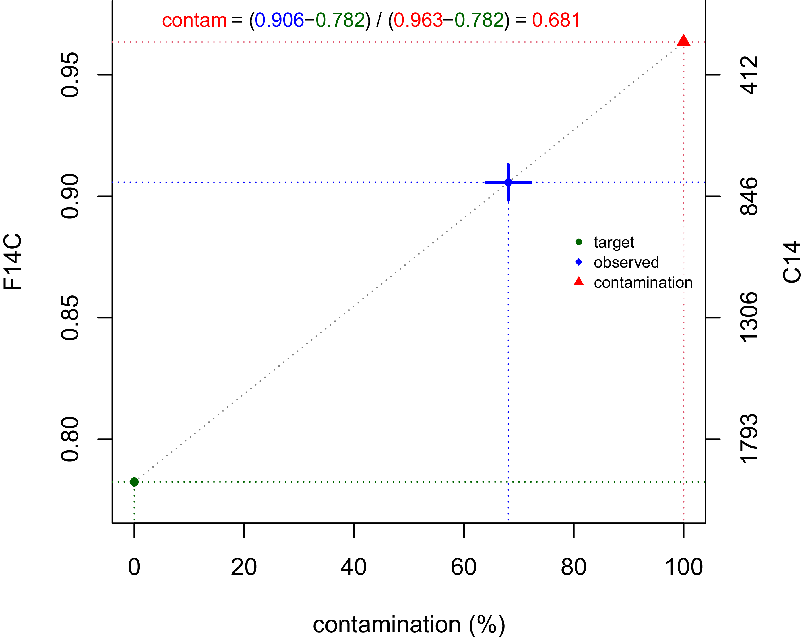
Samples are easily contaminated with non-contemporaneous carbon sources, for example in the field, during storage/preservation, or in the laboratory during sample pretreatment and analysis. Examples include older terrestrial carbon incorporated into marine sediments (e.g. Rosenheim et al. Reference Rosenheim, Day, Domack, Schrum, Benthien and Hayes2008), or finite ages from background samples such as feldspar, anthracite or other material known to be well over 50,000 years old (Vogel et al. Reference Vogel, Nelson and Southon1987). The impacts of contamination with carbon of a certain F14C can be modeled using equation (3) using two components, e.g., contaminate (5000, 20, 5, 1, F.contam=1) ≈ 4661 ± 69 14C BP will model the impact of 5 ± 1% modern contamination (with a F14C of 1) on material dating to 5000 ± 20 14C BP. Similarly, a contaminated date can be ‘cleaned’ of its (5%, modern) contamination: clean (2000, 20, 5, F.contam=1) ≈ 2121 ± 21 14C BP. We can also calculate what percentage (or F14C) of contamination would be required to “explain away” an observed age. E.g., what if the Shroud of Turin really dates to around AD 30 but has been contaminated by carbon from repairs following a known AD 1532 fire? Taking one of the observed Shroud’s 14C dates, Ox-2575.1, we can see that this sample would need to be contaminated by c. 68% of AD 1532 material (see Figure 3). The muck function can also be used to estimate the required F14C of the contamination if its percentage is known. The contaminate, clean and muck functions use Monte Carlo sampling by default to estimate uncertainties (therefore, slight output variations may exist across multiple runs).
Amount of contamination (horizontal axis) versus F14C (left axis) and 14C age (right axis; logarithmic). The target age (green; AD 30 = 1971 ± 15 14C BP = 0.782 ± 0.001 F14C) has 0% contamination, whereas the x position of 100% shows the “pure” contamination (red, here assumed to be of age AD 1532 = 0.963 ± 0.001 F14C). Working on the F14C scale, the observed age (blue, Ox-2575.1 = 795 ± 65 14C BP = 0.906 ± 0.007 F14C) can be visualized as lying on a straight line between the target and contamination, and the resulting percentage contamination can be estimated at c. 68.2%.

Marine offsets
Radiocarbon dates on oceanic material tend to have older radiocarbon ages than contemporaneous terrestrial material and require calibration with the marine calibration curve (Heaton et al. Reference Heaton, Köhler, Butzin, Bard, Reimer, Austin, Bronk Ramsey, Grootes, Hughen, Kromer, Reimer, Adkins, Burke, Cook, Olsen and Skinner2020, Reference Heaton, Butzin, Bard, Bronk Ramsey, Hughen, Köhler and Reimer2023; Keith and Anderson Reference Keith and Anderson1963). Besides this global marine offset, ocean circulation patterns including upwelling cause local or regional marine offsets, which have been estimated in many coastal regions by 14C dating shells that were collected before bomb 14C influence (Reimer and Reimer Reference Reimer and Reimer2001). A copy of the marine reservoir correction databaseFootnote 10 (Reimer and Reimer Reference Reimer and Reimer2001) is available within rice. It can be queried using, e.g., Atlantic <- find.shells(-6, 45, 50) which will return a map and the details of the 50 shells closest to 6° west and 45° north (Figure 4; alternatively, supply the longitude and latitude ranges through map.shells). Optionally, the data can be plotted on a browsable satellite map (setting browse=TRUE), and ocean currents for the region can be shown separatelyFootnote 11. The output can be made to return only shells with certain feeding ecologies, e.g., map.shells(-6, 45, feeding=″suspension″). Weighted means can be calculated from multiple shells, using for example Brazil <- map.shells(-30, -60, 0, -30); shells.mean(Brazil) ≈ −118 ± 113 (the reported error is the maximum of the weighted uncertainty and the standard deviation).
A map of shell-based estimates of the regional marine reservoir offset. Red-to-yellow gradient shows ΔR, symbols show feeding ecology. Data were downloaded from the marine database (Reimer and Reimer Reference Reimer and Reimer2001) with ΔR based on Marine20 (Heaton et al. Reference Heaton, Köhler, Butzin, Bard, Reimer, Austin, Bronk Ramsey, Grootes, Hughen, Kromer, Reimer, Adkins, Burke, Cook, Olsen and Skinner2020).

Where relevant, rice functions return their output to enable subsequent analysis, e.g., oldwood <- push.gamma(2450,30,20,2); plot(oldwood$shifted). Some of the functions are available as online applicationsFootnote 12.
The figures in this manuscript were produced using the following rice commands:
Discussion
The rice package has been designed to make it easier to analyse and interpret radiocarbon dates within the R platform without the need to switch between applications such as Internet browsers and spreadsheets.
Many radiocarbon-related calculations such as calibration, correction for reservoir offsets, stratigraphical modeling (Blaauw et al. Reference Blaauw, Aquino-López and Christen2026), age-depth modeling (BChron [Haslett and Parnell Reference Haslett and Parnell2008], clam [Blaauw Reference Blaauw2010], or Bacon [Blaauw and Christen Reference Blaauw and Christen2011]) and dates-as-data (rcarbon [Crema and Bevan Reference Crema and Bevan2021], Heaton et al. Reference Heaton, Al-Assam and Bard2025) can now be performed within the same software environment R. For example, if some 14C dates within a sediment core stem from marine material, are of postbomb age or could be contaminated with modern carbon, then rice could be used to correct the dating information prior to age-modeling. Additionally, R scripts can be made available to others so that they can see exactly what was done, thus increasing reproducibility and transparency in research software (Barker et al. Reference Barker, Chue Hong, Katz, Lamprecht, Martinez-Ortiz, Psomopoulos, Harrow, Castro, Gruenpeter, Martinez and Honeyman2022).
The rice package has been tested at training workshops for postgraduate students and other early-career researchers. By showcasing and discussing the functions, the participants were able to quickly cover the basics of radiocarbon dating, calibration and corrections. Some prior experience with R is required, but since R has become widely used in many disciplines (with over 23,000 user-contributed packages available on CRAN), this has gradually become less of an issue.
For future iterations of the package, we are considering adding options such as kriging-based spatial interpolation of ΔR (e.g., Ulm et al. Reference Ulm, O’Grady, Petchey, Hua, Jacobsen, Linnenlucke, David, Rosendahl, Bunbury, Bird and Reimer2023). The open nature of rice enables users to write additional or enhanced functions, either for their own use or for sharing with the wider community.
Conclusion
We developed rice, a flexible toolkit for a range of radiocarbon-related calculations, such as transformation between time-scales and units, modeling carbon sources, and calibration. The toolkit can be used within R, a single, scriptable and open-source environment, both for research and teaching purposes.
Supplementary material
A rice tutorial is available at [Radiocarbon https://doi.org/10.1017/RDC.2026.10221]
Acknowledgment
The authors thank Ron Reimer for useful discussion particularly with regards to the marine radiocarbon reservoir database, and the referees for their helpful comments.
Competing interests
The authors declare that they have no competing interests.




 Open access

