

1 Introduction
Modeling multivariate discrete data is a common problem across many fields, such as social sciences, psychology, and ecology. For instance, in education research, discrete data arises from students’ test scores (Maydeu-Olivares & Liu, Reference Maydeu-Olivares and Liu2015), and in ecology, discrete data arises when the counts of a given animal population are measured over various areas and time periods (Anderson et al., Reference Anderson, de Valpine, Punnett and Miller2019; Maslen et al., Reference Maslen, Popovic, Lim, Marzinelli and Warton2023). As the size of data sets continues to expand, missing data becomes increasingly prevalent (Kang, Reference Kang2013), and it is common to have access to a rich set of discrete variables that is subject to missingness. Both the multivariate discreteness and the missingness alone can create modeling difficulties, but together, they present a unique challenge for statistical inference.
1.1 The National Alzheimer’s Coordinating Center database
Although the general problem statement is widely important, our work is primarily motivated by the analysis of neuropsychological test scores in the database of the National Alzheimer’s Coordinating Center (NACC).Footnote 1 The NACC is an NIH/NIA-funded center that maintains the largest longitudinal database for Alzheimer’s disease in the United States. The NACC coordinates 33 Alzheimer’s Disease and Research Centers (ADRC) in the United States.
In the NACC data, we have 41,181 individuals with data collected from 2005 to 2019. In this study, we are particularly interested in information regarding the neuropsychological tests. The neuropsychological tests are a set of examinations measuring an individual’s cognitive ability in four different domains: language, attention, executive function, and memory. The scores from these tests are important features for dementia research because they are not based on a clinician’s judgment. Similar to a conventional exam, the outcome of a neuropsychological test is a discrete number taking integer values and has a known range. Note that different tests have a different ranges. In our study, we consider eight neuropsychological test scores per individual.
A goal of this article is to introduce a simple and interpretable statistical model for modeling the neuropsychological tests. The discrete and correlated nature of the neuropsychological tests presents a challenge for modeling them. As far as we are aware, there is no statistical model for handling these test scores directly, not to mention the additional challenges from the missingness of the test scores. To simplify the problem, we focus on a static model that only considers the test scores from each individual’s initial visit. While there are many covariates that could be incorporated in the analysis, we choose to include only four demographic variables (age, education, sex, and race) to reduce the complexity of the model. These variables are key demographic variables that are often included in any dementia research.
1.2 Research questions
Because the ranges of exams are generally large (30–300), it is infeasible to nonparametrically model the joint distribution of the eight test scores. Moreover, we have demographic variables, such as education, age, and sex. It is a nontrivial problem to study the relation between these demographic variables and the test scores. Furthermore, the existence of missing test scores among certain individuals further compounds the complexity of the overall analysis. In this article, our primary focus centers on addressing the following research questions:
-
1. Finding a feasible and interpretable model for multiple discrete outcomes with missing values. As mentioned before, our data contain multiple dependent discrete variables with missing values. We need to design a proper model to model the dependency among discrete variables and deal with the missing data problem. We also need an estimation and inference procedure that quantifies the uncertainty in the model while properly accounting for the missing data in a statistically principled way.
-
2. Discovering latent groups of individuals using neuropsychological tests. Clinicians have developed a set of rules to categorize individuals into different clinical groups (normal cognition, MCI, and dementia). However, this rule is based on clinical judgments and does not involve any neuropsychological information. Clustering has been of interest to the dementia research community (Alashwal et al., Reference Alashwal, El Halaby, Crouse, Abdalla and Moustafa2019). Thus, an ideal model should be able to cluster individuals into groups using neuropsychological test scores that represent multiple cognitive domains of interest.
-
3. Investigating the association between neuropsychological tests and other variables. It is often of a lot of interest to study how neuropsychological tests are associated with demographic variables or clinical judgments. For instance, there is a hypothesis that people with a higher education are more resilient to cognitive decline as a form of cognitive reserve (Meng & D’Arcy, Reference Meng and D’Arcy2012; Thow et al., Reference Thow, Summers, Saunders, Summers, Ritchie and Vickers2018). We also want to use the NACC data to test this hypothesis.
1.3 Literature review
We provide some background on the current research in Alzheimer’s disease and statistics methodology literature.
1.3.1 Dementia-related research
Multiple outcome variables are common in dementia-related research, but there is no clear widespread solution to the modeling problem. In some previous methods in the Alzheimer’s disease literature, multiple test scores are standardized and averaged into a single holistic score for an individual (Boyle et al., Reference Boyle, Yu, Wilson, Leurgans, Schneider and Bennett2018). This turns the multiple outcome problem into a single outcome problem and ignores the dependence structure. Mjørud et al. (Reference Mjørud, Røsvik, Rokstad, Kirkevold and Engedal2014) examined variables associated with multiple quality-of-life-related discrete outcomes and performed univariate regression on each outcome. Dimension reduction is also commonly used to reduce the number of outcome variables (Qiu et al., Reference Qiu, Jacobs, Messer, Salmon and Feldman2019; Yesavage et al., Reference Yesavage, Taylor, Friedman, Rosenberg, Lazzeroni, Leoutsakos and Group2016), but this can lead to loss of interpretability as any downstream analysis is not using the original variables. Missing data is often ignored completely or when accounted for, single imputation methods or an off-the-shelf imputation approach are typically used (Brenowitz et al., Reference Brenowitz, Hubbard, Keene, Hawes, Longstreth, Woltjer and Kukull2017; Qiu et al., Reference Qiu, Jacobs, Messer, Salmon and Feldman2019).
Clustering has also become increasingly valuable in the dementia research community (Alashwal et al., Reference Alashwal, El Halaby, Crouse, Abdalla and Moustafa2019). For example, Escudero et al. (Reference Escudero, Zajicek and Ifeachor2011) used the K-means algorithm to divide subjects into pathologic and non-pathologic groups to study the early detection of Alzheimer’s disease. Tosto et al. (Reference Tosto, Monsell, Hawes, Bruno and Mayeux2016) used K-means on a subset of NACC data to identify subgroups within Alzheimer’s disease patients to understand the heterogeneity of the disease. Several papers also described model-based clustering approaches. For example, De Meyer et al. (Reference De Meyer, Shapiro, Vanderstichele, Vanmechelen, Engelborghs, De Deyn and Initiative2010) clustered biomarker data using a simple two-component Gaussian mixture model for early detection of Alzheimer’s disease. Qiu et al. (Reference Qiu, Jacobs, Messer, Salmon and Feldman2019) used neuropsychological test scores from a smaller data set than ours, imputing missing data using single imputation methods and the mice R package (van Buuren & Groothuis-Oudshoorn, Reference van Buuren and Groothuis-Oudshoorn2011). Then, they applied principal components analysis before finally, using a Gaussian mixture model for clustering. In our work, we choose to model the raw test scores to avoid loss of information and preserve more interpretability. It is crucial to be cautious when employing single imputation methods or off-the-shelf packages, as they can potentially lead to an underestimation of the uncertainty associated with missing data, and the underlying assumptions regarding missing data may remain unclear.
Additionally, the cognitive reserve hypothesis emerged several decades ago when it was observed that after autopsies, some individuals with no dementia symptoms had brains that exhibited advanced Alzheimer’s pathology (Katzman et al., Reference Katzman, Aronson, Fuld, Kawas, Brown, Morgenstern and Ooi1989). Researchers hypothesized that some activities in life may provide individuals with a given resilience to cognitive decline, which is known as the cognitive reserve hypothesis. As such, there is deep interest in discovering the association between various covariates and dementia (Meng & D’Arcy, Reference Meng and D’Arcy2012; Stern, Reference Stern2012; Thow et al., Reference Thow, Summers, Saunders, Summers, Ritchie and Vickers2018; Zhang et al., Reference Zhang, Katzman, Salmon, Jin, Cai, Wang, Qu, Grant, Yu, Levy and Klauber1990).
1.3.2 Methodology research
This article sits at the intersection of multiple subfields of statistics, including latent variable modeling, missing data, and clustering. The latent class model (LCM) was first proposed by Goodman (Reference Goodman1974) for the purpose of modeling multivariate discrete data. The basic form of the LCM is of a mixture of multivariate multinomials. When the number of levels of the discrete random variable is large, this can lead to a large number of parameters (Bouveyron et al., Reference Bouveyron, Celeux, Murphy and Raftery2019). There has been much work studying many aspects of the LCM, including the identifiability (Allman et al., Reference Allman, Matias and Rhodes2009; Carreira-Perpinan & Renals, Reference Carreira-Perpinan and Renals2000; Gu & Xu, Reference Gu and Xu2020; Gyllenberg et al., Reference Gyllenberg, Koski, Reilink and Verlaan1994) and incorporation of covariates (Huang & Bandeen-Roche, Reference Huang and Bandeen-Roche2004; Ouyang & Xu, Reference Ouyang and Xu2022; Vermunt, Reference Vermunt2010). The traditional LCM has been extended in various forms, such as a mixture of Rasch models (Rost, Reference Rost1990) and a mixture of item response models (McParland & Gormley, Reference McParland, Gormley, Lausen, Van den Poel and Ultsch2013).
The mixture of expert models is closely related to the mixture model framework and the LCM (Jacobs et al., Reference Jacobs, Jordan, Nowlan and Hinton1991). It generalizes the standard mixture model by allowing the parameters to potentially depend on covariates (Gormley & Frühwirth-Schnatter, Reference Gormley and Frühwirth-Schnatter2018). The increased flexibility of the models is associated with a large increase in the number of parameters. Many estimation procedures have been explored, including those based on an EM approach (Jacobs et al., Reference Jacobs, Jordan, Nowlan and Hinton1991; Jordan & Jacobs, Reference Jordan and Jacobs1993), an EMM approach (Gormley & Murphy, Reference Gormley and Murphy2008), or a Bayesian framework (Bishop & Svenskn, Reference Bishop and Svenskn2002; Fruhwirth-Schnatter & Kaufmann, Reference Fruhwirth-Schnatter and Kaufmann2008).
Clustering has previously been explored in combination with missing data. Lee & Harel (Reference Lee and Harel2022) proposed a two-stage clustering framework by first clustering multiply imputed data sets individually and then, obtaining a final clustering by clustering the set of cluster centers obtained over all imputed data sets. In previous research on model-based clustering with missing data, Serafini et al. (Reference Serafini, Murphy and Scrucca2020) employed the EM algorithm and Monte Carlo methods to estimate Gaussian mixture models in the presence of missing at random (MAR) data. Sportisse et al. (Reference Sportisse, Marbac, Biernacki, Boyer, Celeux, Josse and Laporte2024) addressed model-based clustering under missing-not-at-random (MNAR) assumptions, employing a likelihood-based approach and EM algorithm. We include further comments on these methods in Appendix D of the Supplementary Material. These methods addressed the clustering problem but did not use covariates or discuss quantifying the uncertainty of the parameters. Since our method is motivated by the statistical analysis of Alzheimer’s disease, handling both of these is critical to our work.
1.4 Outline
Our article is organized as follows. Section 2 presents a detailed description of our mixture of binomial product experts model. The handling of missing data is discussed in Section 3, where we describe the fitting of the model under a nonmonotone MAR assumption. In Section 4, we delve into the process of inference, specifically in constructing confidence intervals for the parameters of interest. We outline how to perform clustering in Section 5. In Section 6, we provide simulation results to examine the consistency and the coverage of our proposed estimator. In Section 7, we apply our method to an Alzheimer’s disease data set, which motivates our model formulation. Finally, Section 8 concludes the article with a discussion of the results. In the Supplementary Material, we include further details on derivations and proofs (Appendices A and H of the Supplementary Material), identification theory (Appendix B of the Supplementary Material), code implementation (Appendix C of the Supplementary Material), remarks on related EM algorithms (Appendix D of the Supplementary Material), simulations (Appendix E of the Supplementary Material), comments on model selection (Appendix F of the Supplementary Material), comments on clustering (Appendix G of the Supplementary Material), and more comments on the real data analysis (Appendix I of the Supplementary Material). We provide a code implementation of our method in an R package.
2 Mixture of binomial product experts
2.1 A latent class model for neuropsychological test scores
Suppose we have n IID observations, indexed by $i=1,\ldots ,n$
. Let
$i=1,\ldots ,n$
. Let $\textbf {X}_i = (X_{i,1}, X_{i,2}, \ldots , X_{i,p})^\top \in \mathcal {X}\subset \mathbb {R}^p$
be the covariates and
$\textbf {X}_i = (X_{i,1}, X_{i,2}, \ldots , X_{i,p})^\top \in \mathcal {X}\subset \mathbb {R}^p$
be the covariates and $\textbf {Y}_i = (Y_{i,1}, Y_{i,2},\ldots , Y_{i,d})^\top \in \mathcal {Y} \subset \mathbb {Z}^d$
be the outcome variables of interest, where
$\textbf {Y}_i = (Y_{i,1}, Y_{i,2},\ldots , Y_{i,d})^\top \in \mathcal {Y} \subset \mathbb {Z}^d$
be the outcome variables of interest, where $\mathcal {Y}$
is a bounded discrete set. In the present study,
$\mathcal {Y}$
is a bounded discrete set. In the present study, $\textbf {Y}_i$
represents the neuropsychological test scores of individual i for a total of d total tests, but this framework can be applied to other problems as well. In the article, for notational convenience, we may elect to drop the index i to simplify notation and refer to the generic random variable that is not associated with a specific individual. The jth test score/outcome variable
$\textbf {Y}_i$
represents the neuropsychological test scores of individual i for a total of d total tests, but this framework can be applied to other problems as well. In the article, for notational convenience, we may elect to drop the index i to simplify notation and refer to the generic random variable that is not associated with a specific individual. The jth test score/outcome variable $Y_j$
belongs to the set
$Y_j$
belongs to the set $\{0,1,2,\ldots ,N_j\}$
. We assume that the covariates are always observed and that only the outcomes may be subject to missingness.
$\{0,1,2,\ldots ,N_j\}$
. We assume that the covariates are always observed and that only the outcomes may be subject to missingness.
We start with a simpler scenario in which the data are completely observed (no absence of any outcome variables). The more complicated setting with missing outcome variables is addressed in Section 3. When we have multiple discrete outcome variables, the nonparametric approach is not feasible due to the curse of dimensionality. To see this, suppose we have four outcome variables, and each outcome variable has ten possible values. The joint distribution has a dimension of $10^4$
, surpassing the order of magnitude of moderately sized samples. This motivates to use a parametric model.
$10^4$
, surpassing the order of magnitude of moderately sized samples. This motivates to use a parametric model.
To model the dependency among discrete variables, we consider a mixture model, which is based on the idea of the LCM. Originally presented in its modern form by Goodman (Reference Goodman1974), the LCM takes the form of the following mixture of multivariate multinomials distribution:
 $$ \begin{align} p(y; \theta) = \sum_{k=1}^K w_k p_k(y; \theta_k) = \sum_{k=1}^K w_k \prod_{j=1}^d p_{k,j}(y_{j}; \theta_{k,j}), \end{align} $$
where $p_{k,j}$
denotes a multinomial with
$p_{k,j}$
denotes a multinomial with $\theta _{k,j}$
being its the parameter and the
$\theta _{k,j}$
being its the parameter and the $w_k$
’s are probability weights for each component such that
$w_k$
’s are probability weights for each component such that $\sum _k w_k = 1$
and
$\sum _k w_k = 1$
and $w_k>0$
for all k. As
$w_k>0$
for all k. As $p_{k,j}$
is a multinomial distribution,
$p_{k,j}$
is a multinomial distribution, $\theta _{k,j}$
refers to the vector of probabilities (one for each level of
$\theta _{k,j}$
refers to the vector of probabilities (one for each level of $Y_j$
) that sum to 1. There is a popular implementation for fitting these models through the poLCA package (Linzer & Lewis, Reference Linzer and Lewis2011).
$Y_j$
) that sum to 1. There is a popular implementation for fitting these models through the poLCA package (Linzer & Lewis, Reference Linzer and Lewis2011).
Let Z denote the component assignment such that $Z = \ell $
if and only if the associated observation is generated from mixture component
$Z = \ell $
if and only if the associated observation is generated from mixture component $\ell $
. Namely,
$\ell $
. Namely, $P(Y=y|Z= k;\theta ) = \prod _{j=1}^d p_{k,j}(y_{j}; \theta _{k,j})$
. By construction, the LCM implicitly assumes that for
$P(Y=y|Z= k;\theta ) = \prod _{j=1}^d p_{k,j}(y_{j}; \theta _{k,j})$
. By construction, the LCM implicitly assumes that for $j\neq j'$
, the variables
$j\neq j'$
, the variables $Y_j$
and
$Y_j$
and $Y_{j'}$
are conditionally independent given the latent class Z. This is known as the local independence assumption and is commonly used in the literature to model dependence between discrete random variables. While they are conditionally independent, the variables
$Y_{j'}$
are conditionally independent given the latent class Z. This is known as the local independence assumption and is commonly used in the literature to model dependence between discrete random variables. While they are conditionally independent, the variables $Y_j$
and
$Y_j$
and $Y_{j'}$
are allowed to depend marginally for
$Y_{j'}$
are allowed to depend marginally for $j\neq j'$
. The local independence assumption makes it convenient to calculate the conditional distributions, which are used in Section 3 when we discuss imputation. Some effort has been made to relax the local independence assumption, such as mixtures of log-linear models (Bock, Reference Bock, Bozdogan, Sclove, Gupta, Haughton, Kitagawa, Ozaki and Tanabe1994) and hierarchical LCMs (Chen et al., Reference Chen, Zhang, Liu, Poon and Wang2012; Zhang, Reference Zhang2004), but these have not been as widely adopted due to the increase in the number of parameters.
$j\neq j'$
. The local independence assumption makes it convenient to calculate the conditional distributions, which are used in Section 3 when we discuss imputation. Some effort has been made to relax the local independence assumption, such as mixtures of log-linear models (Bock, Reference Bock, Bozdogan, Sclove, Gupta, Haughton, Kitagawa, Ozaki and Tanabe1994) and hierarchical LCMs (Chen et al., Reference Chen, Zhang, Liu, Poon and Wang2012; Zhang, Reference Zhang2004), but these have not been as widely adopted due to the increase in the number of parameters.
Throughout this article, we will refer to the data set containing tuples of the form $(\textbf {X},\textbf {Y})$
as the latent incomplete (LI) data and the data set containing tuples of the form
$(\textbf {X},\textbf {Y})$
as the latent incomplete (LI) data and the data set containing tuples of the form $(\textbf {X},\textbf {Y},Z)$
as the latent complete (LC) data. In the setting of no missing data, the LI data are what we typically have access to, but this is often insufficient for direct model fitting due to the unobserved latent variable Z. We will show that one can estimate the model parameters using an EM algorithm with the LI data. We use this nomenclature to avoid confusion in Section 3 when we encounter the traditional type of missingness with the outcome variables.
$(\textbf {X},\textbf {Y},Z)$
as the latent complete (LC) data. In the setting of no missing data, the LI data are what we typically have access to, but this is often insufficient for direct model fitting due to the unobserved latent variable Z. We will show that one can estimate the model parameters using an EM algorithm with the LI data. We use this nomenclature to avoid confusion in Section 3 when we encounter the traditional type of missingness with the outcome variables.
There has been previous work to incorporate covariates in the LCM (Huang & Bandeen-Roche, Reference Huang and Bandeen-Roche2004; Vermunt, Reference Vermunt2010). This is related to the mixture of experts models that arose from the machine learning literature (Jacobs et al., Reference Jacobs, Jordan, Nowlan and Hinton1991; Jordan & Jacobs, Reference Jordan and Jacobs1993; Yuksel et al., Reference Yuksel, Wilson and Gader2012). These models generalize the classical mixture model formulation by allowing the model parameters $w_k$
and
$w_k$
and $\theta _k$
to depend on covariates. The simple mixture of experts model (Gormley & Frühwirth-Schnatter, Reference Gormley and Frühwirth-Schnatter2018) takes the following form:
$\theta _k$
to depend on covariates. The simple mixture of experts model (Gormley & Frühwirth-Schnatter, Reference Gormley and Frühwirth-Schnatter2018) takes the following form:
 $$ \begin{align*} p(y | x; \boldsymbol{\theta}) = \sum_{k=1}^K w_k(x;\beta_k) p_k(y; \theta_k), \end{align*} $$
where $\beta _k$
is introduced to allow the weights to depend on covariates. As written, the covariates only adjust the weights placed on each mixture component but do not affect the parameters of the individual component distribution.
$\beta _k$
is introduced to allow the weights to depend on covariates. As written, the covariates only adjust the weights placed on each mixture component but do not affect the parameters of the individual component distribution.
To apply these ideas to the neuropsychological data, we combine the mixture of experts and LCM, leading to the following mixture of binomial product experts:
 $$ \begin{align} p(y|x; \boldsymbol{\beta}, \boldsymbol{\theta}) = \sum_{k=1}^K w_k(x;\beta_k) \underbrace{\prod_{j=1}^d \underbrace{\binom{N_j}{y_j} (\theta_{k,j})^{y_j} (1-\theta_{k,j})^{N_j-y_j}}_{p_{k,j}(y_j;\theta_{k,j})}}_{p_k(y;\theta_k)}, \end{align} $$
where $w_k(x;\beta _k) = \exp (\beta _k^\top \cdot (1,x)) / (\sum _{k'\in [K]} \exp (\beta _{k'}^\top \cdot (1,x)))$
is from the multiple-class logistic regression model. Like in the classical LCM, we utilize the local independence assumption as each mixture decomposes as a product of binomials. However, there is a critical difference between our model and the classical LCM. We use the binomial distribution instead of the multinomial distribution, and this leads to a large reduction in the number of parameters. Since test scores are ordered variables, we expect the reduction to a binomial distribution to be reasonable as scores further away from the mean score can be less likely. Similar to the simple mixture of experts model, each mixture weight depends on covariates.
$w_k(x;\beta _k) = \exp (\beta _k^\top \cdot (1,x)) / (\sum _{k'\in [K]} \exp (\beta _{k'}^\top \cdot (1,x)))$
is from the multiple-class logistic regression model. Like in the classical LCM, we utilize the local independence assumption as each mixture decomposes as a product of binomials. However, there is a critical difference between our model and the classical LCM. We use the binomial distribution instead of the multinomial distribution, and this leads to a large reduction in the number of parameters. Since test scores are ordered variables, we expect the reduction to a binomial distribution to be reasonable as scores further away from the mean score can be less likely. Similar to the simple mixture of experts model, each mixture weight depends on covariates.
Here, we will treat $k=1$
as the reference group, so
$k=1$
as the reference group, so $\beta _1$
is the vector of all
$\beta _1$
is the vector of all $0$
by assumption and does not need to be estimated. For
$0$
by assumption and does not need to be estimated. For $k \in \{2,3,\ldots ,K\}$
,
$k \in \{2,3,\ldots ,K\}$
, $\beta _k \in \mathbb {R}^{p+1}$
, and for
$\beta _k \in \mathbb {R}^{p+1}$
, and for $k\in [K]$
,
$k\in [K]$
, $\theta _k \in \mathbb {R}^d$
, we assume that the
$\theta _k \in \mathbb {R}^d$
, we assume that the $w_k$
utilize the logistic function, but it is possible to use other link functions, such as the probit and other monotonic functions (Ouyang & Xu, Reference Ouyang and Xu2022). In our work, the outcome variables are neuropsychological test scores, and we treat the latent groups as subgroups of the population of varying cognitive ability. The five levels of the CDR score offer a natural choice for the number of mixture components.
$w_k$
utilize the logistic function, but it is possible to use other link functions, such as the probit and other monotonic functions (Ouyang & Xu, Reference Ouyang and Xu2022). In our work, the outcome variables are neuropsychological test scores, and we treat the latent groups as subgroups of the population of varying cognitive ability. The five levels of the CDR score offer a natural choice for the number of mixture components.
In our model construction, we view each mixture component as representing a subgroup of the population, where the subgroups have varying cognitive ability that is summarized by $\boldsymbol {\theta }$
. Therefore, we interpret the
$\boldsymbol {\theta }$
. Therefore, we interpret the $\boldsymbol {\theta }$
’s as attributes of population-level groups and do not allow them to depend on covariates. Since the weights
$\boldsymbol {\theta }$
’s as attributes of population-level groups and do not allow them to depend on covariates. Since the weights $w_k(x;\beta _k)$
depend on covariates, every individual has their own weights associated with each population-level group. These covariates can be interpreted as a way to construct weights on an individual level for each of these population-level subgroups. A side product of this assumption is that this reduces model complexity. If the
$w_k(x;\beta _k)$
depend on covariates, every individual has their own weights associated with each population-level group. These covariates can be interpreted as a way to construct weights on an individual level for each of these population-level subgroups. A side product of this assumption is that this reduces model complexity. If the $\boldsymbol {\theta }$
’s depend on covariates, then the number of parameters increases from
$\boldsymbol {\theta }$
’s depend on covariates, then the number of parameters increases from $O(K(d + p))$
to
$O(K(d + p))$
to $O(Kdp)$
, which is a dramatic change even for moderately sized d and p and thus another reason we do not allow this as part of our model. Because the outcome variables are test scores, we can also interpret the quantity
$O(Kdp)$
, which is a dramatic change even for moderately sized d and p and thus another reason we do not allow this as part of our model. Because the outcome variables are test scores, we can also interpret the quantity $N_j \cdot \theta _{k,j}$
as the mean of the jth test score of the kth latent group, and this is useful as a summary statistic for a given latent class.
$N_j \cdot \theta _{k,j}$
as the mean of the jth test score of the kth latent group, and this is useful as a summary statistic for a given latent class.
Binomial product distributions have previously arisen in the literature. One such application was for modeling test scores for spatial tasks in child development in Thomas et al. (Reference Thomas, Lohaus and Brainerd1993), but they considered a fairly limited setting with no covariates, two components, and two outcome variables. Binomial product and Poisson product distributions have also been used in the statistical ecology literature to model species abundance (Brintz et al., Reference Brintz, Fuentes and Madsen2018; Haines, Reference Haines2016; Kéry et al., Reference Kéry, Royle and Schmid2005). These settings differ from ours because they often treat the total number counts $N_j$
as a random quantity. In item response theory (IRT), the Rasch model posits that the probability of answering each question correctly depends on its difficulty and the individual’s ability, assuming a Bernoulli distribution for each question (Rasch, Reference Rasch1960). However, in our data, only total test scores are available. Thus, assuming uniform difficulty across test questions, we model the scores using Binomial distributions. To our knowledge, our article is the first time binomial products has been used to analyze neuropsychological test score data while incorporating covariates.
$N_j$
as a random quantity. In item response theory (IRT), the Rasch model posits that the probability of answering each question correctly depends on its difficulty and the individual’s ability, assuming a Bernoulli distribution for each question (Rasch, Reference Rasch1960). However, in our data, only total test scores are available. Thus, assuming uniform difficulty across test questions, we model the scores using Binomial distributions. To our knowledge, our article is the first time binomial products has been used to analyze neuropsychological test score data while incorporating covariates.
Note that for the kth component, $\beta _k \in \mathbb {R}^{p+1}$
and
$\beta _k \in \mathbb {R}^{p+1}$
and $\theta _k \in \mathbb {R}^d$
, there are
$\theta _k \in \mathbb {R}^d$
, there are $(K-1)(p+1)$
parameters associated with the covariates
$(K-1)(p+1)$
parameters associated with the covariates $\boldsymbol {\beta }$
and
$\boldsymbol {\beta }$
and $Kd$
parameters associated with
$Kd$
parameters associated with $\boldsymbol {\theta }$
and a total of
$\boldsymbol {\theta }$
and a total of $K(p+d+1)-p-1$
parameters for the whole model. Thus, for fixed covariate and outcome dimensions, the number of parameters grows linearly in K.
$K(p+d+1)-p-1$
parameters for the whole model. Thus, for fixed covariate and outcome dimensions, the number of parameters grows linearly in K.
2.2 Model fitting
We now describe our procedure for fitting the model. An intuitive approach is to estimate the parameters via the maximum likelihood approach. However, computing the maximum likelihood estimator (MLE) is a nontrivial task because the LI log-likelihood is not concave (Lemma 1 in the Supplementary Material). As such, solving the first-order conditions is no longer sufficient for determining the global maximizer.
Due to Lemma 1 (stated formally in Appendix H.1 of the Supplementary Material), maximizing the LI log-likelihood function directly is not straightforward. Here is an interesting insight from the mixture model literature: if we had access to the latent class label, then the MLE would be easy to construct. This insight motivates us to develop an EM algorithm (Dempster et al., Reference Dempster, Laird and Rubin1977) by augmenting the observed data with the true component label Z to calculate the MLE for $(\boldsymbol {\beta }, \boldsymbol {\theta })$
. For each
$(\boldsymbol {\beta }, \boldsymbol {\theta })$
. For each $i=1,\ldots ,n$
, let
$i=1,\ldots ,n$
, let $Z_i = \ell $
if the ith observation comes from mixture component
$Z_i = \ell $
if the ith observation comes from mixture component $\ell $
. Such data augmentation allows one to bypass the problem of taking the logarithm of a sum. To see this, let
$\ell $
. Such data augmentation allows one to bypass the problem of taking the logarithm of a sum. To see this, let $\textbf {X}_{1:n} = (\textbf {X}_1, \ldots , \textbf {X}_n)$
and
$\textbf {X}_{1:n} = (\textbf {X}_1, \ldots , \textbf {X}_n)$
and $\textbf {Y}_{1:n} = (\textbf {Y}_1, \ldots , \textbf {Y}_n)$
be the covariates and outcome variables of all n individuals, respectively. The LC log-likelihood function is written as
$\textbf {Y}_{1:n} = (\textbf {Y}_1, \ldots , \textbf {Y}_n)$
be the covariates and outcome variables of all n individuals, respectively. The LC log-likelihood function is written as
 $$ \begin{align} \ell_{\text{LC},n}&(\beta, \theta; \textbf{X}_{1:n}, \textbf{Y}_{1:n}, \textbf{Z}_{1:n}) = \log \left( \prod_{i=1}^n \prod_{k=1}^K \left(w_k(\textbf{X}_i; \beta_k) p_k(\textbf{Y}_i; \theta_k)\right)^{1(Z_i=k)}\right) \nonumber \\ &= \sum_{i=1}^n\sum_{k=1}^K 1(Z_i=k) \log w_k(\textbf{X}_i;\beta_k) + \sum_{i=1}^n\sum_{k=1}^K 1(Z_i=k)\log p_k(\textbf{Y}_i;\theta_k). \end{align} $$
In the EM algorithm, we start from an initial guess $(\hat {\boldsymbol {\beta }}^{(0)}, \hat {\boldsymbol {\theta }}^{(0)})$
and iterate between an expectation step (E-step) and a maximization step (M-step) to update our guess until convergence. Let t denote the tth iteration of the EM algorithm. In the E-step, we compute the expected value of the complete log-likelihood
$(\hat {\boldsymbol {\beta }}^{(0)}, \hat {\boldsymbol {\theta }}^{(0)})$
and iterate between an expectation step (E-step) and a maximization step (M-step) to update our guess until convergence. Let t denote the tth iteration of the EM algorithm. In the E-step, we compute the expected value of the complete log-likelihood $\ell _{\text {LC}}(\boldsymbol {\beta }, \boldsymbol {\theta }; \textbf {X},\textbf {Y},\textbf {Z})$
conditional on the observed data
$\ell _{\text {LC}}(\boldsymbol {\beta }, \boldsymbol {\theta }; \textbf {X},\textbf {Y},\textbf {Z})$
conditional on the observed data $\textbf {X}$
and
$\textbf {X}$
and $\textbf {Y}$
. The expected value of the LC log-likelihood given the observed data forms the Q function in the EM algorithm
$\textbf {Y}$
. The expected value of the LC log-likelihood given the observed data forms the Q function in the EM algorithm
 $$\begin{align*}Q_{\text{LC}}(\boldsymbol{\beta}, \boldsymbol{\theta} | \textbf{X}, \textbf{Y}; \hat{\boldsymbol{\beta}}^{(t)}, \hat{\boldsymbol{\theta}}^{(t)}) := \mathbb{E}[\ell_{\text{LC}}(\boldsymbol{\beta}, \boldsymbol{\theta}; \textbf{X},\textbf{Y},Z) | \textbf{X}, \textbf{Y}; \hat{\boldsymbol{\beta}}^{(t)}, \hat{\boldsymbol{\theta}}^{(t)}] . \end{align*}$$
In practice, we do not have access to the true expectation, so we work with the sample analog $Q_{\text {LC},n}$
. The sample analog can be expressed as
$Q_{\text {LC},n}$
. The sample analog can be expressed as
 $$ \begin{align} &Q_{\text{LC}, n}(\boldsymbol{\beta}, \boldsymbol{\theta} | \textbf{X}_{1:n}, \textbf{Y}_{1:n}; \hat{\boldsymbol{\beta}}^{(t)}, \hat{\boldsymbol{\theta}}^{(t)}) \nonumber \\ &:= \frac{1}{n}\sum_{i=1}^n\sum_{k=1}^K \hat{\pi}_k^{(t)}(\textbf{X}_i, \textbf{Y}_i) \log w_k(\textbf{X}_i;\beta_k) + \frac{1}{n}\sum_{i=1}^n\sum_{k=1}^K \hat{\pi}_k^{(t)}(\textbf{X}_i, \textbf{Y}_i) \log p_k(\textbf{Y}_i;\theta_k), \end{align} $$
where
 $$ \begin{align} \hat{\pi}_k^{(t)}(\textbf{X}_i, \textbf{Y}_i) := P(Z=k|\textbf{X}_i,\textbf{Y}_i; \hat{\boldsymbol{\beta}}^{(t)}, \hat{\boldsymbol{\theta}}^{(t)}) = \frac{w_k(\textbf{X}_i;\hat{\beta}_k^{(t)}) p_k(\textbf{Y}_i; \hat{\theta}_k^{(t)})}{\sum_{k'=1}^K w_{k'}(\textbf{X}_i;\hat{\beta}_{k'}^{(t)}) p_{k'}(\textbf{Y}_i; \hat{\theta}_{k'}^{(t)})} \end{align} $$
is the weight of observation $(\textbf {X}_i, \textbf {Y}_i)$
for the kth mixture component.
$(\textbf {X}_i, \textbf {Y}_i)$
for the kth mixture component.
Since the LC log-likelihood function (2.3) decomposes as the sum of a function of $\boldsymbol {\beta }$
and a function of
$\boldsymbol {\beta }$
and a function of $\boldsymbol {\theta }$
, the maximization step of the EM algorithm is separable. Note that since
$\boldsymbol {\theta }$
, the maximization step of the EM algorithm is separable. Note that since $w_k$
and
$w_k$
and $p_k$
are logistic regression and binomial product models, respectively, one can apply standard off-the-shelf model fitting procedures after reweighting each observation i by
$p_k$
are logistic regression and binomial product models, respectively, one can apply standard off-the-shelf model fitting procedures after reweighting each observation i by $\hat {\pi }_k^{(t)}(\textbf {X}_i,\textbf {Y}_i)$
. In the maximization step, the new estimate for
$\hat {\pi }_k^{(t)}(\textbf {X}_i,\textbf {Y}_i)$
. In the maximization step, the new estimate for $\boldsymbol {\theta }$
is updated as follows for each
$\boldsymbol {\theta }$
is updated as follows for each $k\in [K]$
and
$k\in [K]$
and $j \in [d]$
,
$j \in [d]$
,
 $$ \begin{align} \hat{\theta}^{(t+1)}_{k, j} := \dfrac{\sum_{i=1}^n \frac{Y_{i,j}}{N_j} \hat{\pi}_k^{(t)}(\textbf{X}_i, \textbf{Y}_i)}{\sum_{i=1}^n \hat{\pi}_k^{(t)}(\textbf{X}_i, \textbf{Y}_i)}, \end{align} $$
which is simply the standard MLE formed by the sample proportion, reweighted by $\hat {\pi }_k^{(t)}(\textbf {X}_i,\textbf {Y}_i)$
. We update our estimate of
$\hat {\pi }_k^{(t)}(\textbf {X}_i,\textbf {Y}_i)$
. We update our estimate of $\beta _k$
by fitting a multi-class logistic regression by reweighting each corresponding observation by
$\beta _k$
by fitting a multi-class logistic regression by reweighting each corresponding observation by $\hat {\pi }_k^{(t)}(\textbf {X}_i, \textbf {Y}_i)$
. This is equivalent to regressing the variable
$\hat {\pi }_k^{(t)}(\textbf {X}_i, \textbf {Y}_i)$
. This is equivalent to regressing the variable $W^{(t)}$
on the covariates X, where
$W^{(t)}$
on the covariates X, where $W_i^{(t)} = (\hat {\pi }_1^{(t)}(\textbf {X}_i, \textbf {Y}_i), \ldots , \hat {\pi }_K^{(t)}(\textbf {X}_i, \textbf {Y}_i)) \in S^{K-1}$
for all i, where
$W_i^{(t)} = (\hat {\pi }_1^{(t)}(\textbf {X}_i, \textbf {Y}_i), \ldots , \hat {\pi }_K^{(t)}(\textbf {X}_i, \textbf {Y}_i)) \in S^{K-1}$
for all i, where $S^{K-1}$
is the
$S^{K-1}$
is the $(K-1)$
th probability simplex. Note that this is not the standard logistic regression because the outcome variable belongs to a probability simplex. This logistic regression can still be fit using gradient descent in standard R packages.
$(K-1)$
th probability simplex. Note that this is not the standard logistic regression because the outcome variable belongs to a probability simplex. This logistic regression can still be fit using gradient descent in standard R packages.

Algorithm 1 describes the process of fitting the mixture of binomial product experts model in the presence of completely observed covariate and outcome data. For a single initialization point, the EM algorithm is not guaranteed to converge to the global maximizer. In practice, we run Algorithm 1 many times with multiple random initial guesses to explore the parameter space sufficiently and choose the parameter estimate from all of them that maximizes the log-likelihood.
2.3 Identifiability
We now make some brief comments on the identifiability of our model. Identifiability means that each parameter value corresponds to a unique probability distribution. That is, the mapping from the parameter space to the space of probability distributions is one-to-one. If identifiability does not hold, estimation becomes problematic because a unique MLE may not exist. However, this notion of identifiability may be too strong for many practical purposes. For example, even the common problem of label swapping violates this identifiability definition, so researchers often consider the idea of identifiability up to permutation of the parameters. We now consider the notion of generic identifiability, which relaxes the definition of identifiability even further. Generic identifiability means identifiability holds almost everywhere in the parameter space (Allman et al., Reference Allman, Matias and Rhodes2009). More formally, this means that the mapping from the parameter space to the space of probability distributions may fail to be one-to-one only on a set of Lebesgue measure zero. Generic identifiability (holding almost everywhere) can be viewed as an intermediate assumption between two common assumptions: global identifiability (holding everywhere) and local identifiability (holding in a neighborhood of the true parameter). In a practical sense, this means that any such model fit on a given data set is unlikely to be unidentifiable, and we consider this notion to be sufficient for our applied data setting.
Proposition 1 (Sufficient conditions for generic identifiability)
Suppose the following conditions hold:
-
A1 Each mixture is distinct such that $\theta _k \neq \theta _{k'}$
when
$k \neq k'$
.
$\theta _k \neq \theta _{k'}$
when
$k \neq k'$
. -
A2 The number of outcome variables d and the number of mixtures K satisfy the bound
$d \geq 2\lceil \log _{1+\min _j N_j} K \rceil + 1$
. -
A3 The design matrix is full-rank and
$n> p$
.


Then, the mixture of binomial product experts is generically identifiable up to permutation of the parameters.
We note that the sufficient conditions outlined in Proposition 1 are fairly mild. Intuitively, one would not want the number of parameters to be too large when the data dimension d is small. The bound in Assumption A2 ensures that the number of mixture components K remains appropriately controlled relative to d and $N_j$
, as a large K increases model complexity. When there are at least
$N_j$
, as a large K increases model complexity. When there are at least $d=3$
outcome variables of moderate range, K can still be fairly large. Assumption A3 is to ensure identifiability of the logistic regression parameters. We provide further comments on the assumptions and the proof of this proposition in Appendix B of the Supplementary Material. These assumptions are fairly mild, and we show that they can be met using relatively straightforward generating processes through our simulations in Section 6.
$d=3$
outcome variables of moderate range, K can still be fairly large. Assumption A3 is to ensure identifiability of the logistic regression parameters. We provide further comments on the assumptions and the proof of this proposition in Appendix B of the Supplementary Material. These assumptions are fairly mild, and we show that they can be met using relatively straightforward generating processes through our simulations in Section 6.
3 Missingness in the outcome variables
Another challenge in the NACC’s neuropsychological data is the missingness in the outcomes. To properly describe the missing data problem, we first introduce some additional notation. Let $\textbf {R}_i = (R_{i,1}, R_{i,2}, \ldots , R_{i,d})^\top \in \mathcal {R}\subseteq \{0,1\}^d$
be the random binary vector that denotes the missing pattern associated with individual i. Element
$\textbf {R}_i = (R_{i,1}, R_{i,2}, \ldots , R_{i,d})^\top \in \mathcal {R}\subseteq \{0,1\}^d$
be the random binary vector that denotes the missing pattern associated with individual i. Element $R_{i,j}$
of the binary vector
$R_{i,j}$
of the binary vector $\textbf {R}_i$
is
$\textbf {R}_i$
is $1$
if and only if
$1$
if and only if $Y_{i,j}$
is observed. For a given pattern
$Y_{i,j}$
is observed. For a given pattern $r \in \mathcal {R}$
, let
$r \in \mathcal {R}$
, let $\textbf {Y}_{i,r} = (Y_i,j: r_{i,j}=1)$
denote the observed variables and
$\textbf {Y}_{i,r} = (Y_i,j: r_{i,j}=1)$
denote the observed variables and $\textbf {Y}_{i,\bar {r}} = (Y_{i,j}: r_{i,j}=0)$
denote the missing variables. For example, when
$\textbf {Y}_{i,\bar {r}} = (Y_{i,j}: r_{i,j}=0)$
denote the missing variables. For example, when $d=4$
and
$d=4$
and $r=1,001$
, then
$r=1,001$
, then $\textbf {Y}_{i,r} = (Y_{i,1},Y_{i,4})$
and
$\textbf {Y}_{i,r} = (Y_{i,1},Y_{i,4})$
and $\textbf {Y}_{i,\bar {r}} = (Y_{i,2}, Y_{i,3})$
. Similarly, for observation i with random missing pattern
$\textbf {Y}_{i,\bar {r}} = (Y_{i,2}, Y_{i,3})$
. Similarly, for observation i with random missing pattern $\textbf {R}_i$
, denote
$\textbf {R}_i$
, denote $\textbf {Y}_{i,\textbf {R}_i}$
and
$\textbf {Y}_{i,\textbf {R}_i}$
and $\textbf {Y}_{i,\bar {\textbf {R}}_i}$
as the observed and missing outcome variables for the ith observation, respectively. We place no restrictions on the set of possible patterns
$\textbf {Y}_{i,\bar {\textbf {R}}_i}$
as the observed and missing outcome variables for the ith observation, respectively. We place no restrictions on the set of possible patterns $\mathcal {R}$
, allowing the pattern to be nonmonotone. Since
$\mathcal {R}$
, allowing the pattern to be nonmonotone. Since $|\mathcal {R}| \leq 2^d$
, missingness can easily become an exponentially complex problem in the dimension of the outcome variables.
$|\mathcal {R}| \leq 2^d$
, missingness can easily become an exponentially complex problem in the dimension of the outcome variables.
In contrast to the previous section, we will use the term fully complete (FC) to refer to a data set containing IID tuples of the form $(\textbf {X},\textbf {Y},Z,\textbf {R})$
. We call a data set containing IID observations of the form
$(\textbf {X},\textbf {Y},Z,\textbf {R})$
. We call a data set containing IID observations of the form $(\textbf {X},\textbf {Y}_{\textbf {R}},\textbf {R})$
as the observed data. Note that the observed data now have two kinds of incompleteness/missingness: incompleteness in the latent class variable (due to mixture models) and missingness in the outcomes. As the case with the LC data, we also do not have access to the FC data. We collect all of the observed outcome variables in one tuple
$(\textbf {X},\textbf {Y}_{\textbf {R}},\textbf {R})$
as the observed data. Note that the observed data now have two kinds of incompleteness/missingness: incompleteness in the latent class variable (due to mixture models) and missingness in the outcomes. As the case with the LC data, we also do not have access to the FC data. We collect all of the observed outcome variables in one tuple $\textbf {Y}_{1:n, \textbf {R}_{1:n}} = (\textbf {Y}_{1,\textbf {R}_1}, \textbf {Y}_{2,\textbf {R}_2}, \ldots , \textbf {Y}_{n,\textbf {R}_n})$
.
$\textbf {Y}_{1:n, \textbf {R}_{1:n}} = (\textbf {Y}_{1,\textbf {R}_1}, \textbf {Y}_{2,\textbf {R}_2}, \ldots , \textbf {Y}_{n,\textbf {R}_n})$
.
3.1 Missing at random and an imputation strategy
Rubin (Reference Rubin1976) outlined three types of missingness mechanisms: missing completely at random (MCAR), MAR, and MNAR. MCAR assumes that the missingness of the variable is independent of all variables in the data. MAR assumes that the missingness of a variable can only depend on observed variables. MNAR assumes that the missingness of a variable can depend on the value of the variable subject to missingness.
In the MCAR data, model fitting is straightforward because one can run Algorithm 1 on the complete cases, and the estimates of the parameters will be consistent. However, MCAR assumes that the missingness is irrelevant to observed outcomes, which is clearly false in the NACC data as a possible reason to miss some test scores is that the individual was too sick to finish the test. Therefore, we consider the MAR assumption. Formally, the definition of MAR is as follows.
Definition 1 (Missing at random)
The outcome variables $\textbf {Y}$
are MAR if the probability of missingness is dependent only on the variables that are observed for the given pattern. This assumption is written as
$\textbf {Y}$
are MAR if the probability of missingness is dependent only on the variables that are observed for the given pattern. This assumption is written as
 $$ \begin{align} P(\textbf{R}=r | \textbf{X}, \textbf{Y}) \stackrel{\text{MAR}}{=} P(\textbf{R}=r | \textbf{X}, \textbf{Y}_r) \end{align} $$
for all $r\in \mathcal {R}$
.
$r\in \mathcal {R}$
.
Notice that the left-hand side of (3.1) represents the selection probability $P(\textbf {R}=r|\textbf {X},\textbf {Y})$
. This quantity is strictly unidentifiable because it depends on unobserved data, specifically
$P(\textbf {R}=r|\textbf {X},\textbf {Y})$
. This quantity is strictly unidentifiable because it depends on unobserved data, specifically $\textbf {Y}_{\bar {r}}$
. Thus, it cannot be estimated even given infinite observed data. The MAR assumption makes
$\textbf {Y}_{\bar {r}}$
. Thus, it cannot be estimated even given infinite observed data. The MAR assumption makes $P(\textbf {R}=r|\textbf {X},\textbf {Y})$
identifiable because it equates it to a probability
$P(\textbf {R}=r|\textbf {X},\textbf {Y})$
identifiable because it equates it to a probability $P(\textbf {R}=r|\textbf {X},\textbf {Y}_r)$
that can be estimated from the observed data; the variables under the conditioning are all of the variables strictly observed under pattern r. The definition of MAR implies that the probability of a given missing pattern does not depend on variables that are unobserved under that pattern. A key advantage of this assumption is that we avoid the challenge of modeling the joint distribution between
$P(\textbf {R}=r|\textbf {X},\textbf {Y}_r)$
that can be estimated from the observed data; the variables under the conditioning are all of the variables strictly observed under pattern r. The definition of MAR implies that the probability of a given missing pattern does not depend on variables that are unobserved under that pattern. A key advantage of this assumption is that we avoid the challenge of modeling the joint distribution between $\textbf {Y}$
and
$\textbf {Y}$
and $\textbf {R}$
since the missingness mechanism
$\textbf {R}$
since the missingness mechanism $P(\textbf {R}=r|\textbf {X},\textbf {Y})$
does not need to be modeled directly; this is known as the ignorability property (see the discussion later). Thus, we do not have to deal with making potentially unreasonable modeling assumptions on either the selection model
$P(\textbf {R}=r|\textbf {X},\textbf {Y})$
does not need to be modeled directly; this is known as the ignorability property (see the discussion later). Thus, we do not have to deal with making potentially unreasonable modeling assumptions on either the selection model $P(\textbf {R}=r|x,y)$
or the extrapolation distribution
$P(\textbf {R}=r|x,y)$
or the extrapolation distribution $p(y_{\bar {r}} | y_r, x, \textbf {R}=r)$
.
$p(y_{\bar {r}} | y_r, x, \textbf {R}=r)$
.
The MAR assumption is untestable because its validity relies strictly on data that is unobserved, and so it cannot be rejected by the observed data. Our primary reason for selecting this assumption is for modeling. This may lead to easier interpretability for scientists and practitioners since we fit a global model $p(y|x)$
across all missing patterns rather than a local model
$p(y|x)$
across all missing patterns rather than a local model $p(y|x, R = r)$
for every pattern r. In the Alzheimer’s disease literature, having more statistically sound work can be meaningful because of limitations in existing work that we have described previously in Section 1.3.1. Since we believe that it may be plausible because these tests are correlated due to underlying cognitive ability, we can use it as a starting point. This can be viewed as a baseline before proceeding with more complex MNAR assumptions. We recognize that MNAR may be more reasonable since missing test scores may be attributed to sickness. However, this is in itself a very open research question because MNAR is a broad class of assumptions, and performing mixture modeling with MNAR is not straightforward; we leave this for future work.
$p(y|x, R = r)$
for every pattern r. In the Alzheimer’s disease literature, having more statistically sound work can be meaningful because of limitations in existing work that we have described previously in Section 1.3.1. Since we believe that it may be plausible because these tests are correlated due to underlying cognitive ability, we can use it as a starting point. This can be viewed as a baseline before proceeding with more complex MNAR assumptions. We recognize that MNAR may be more reasonable since missing test scores may be attributed to sickness. However, this is in itself a very open research question because MNAR is a broad class of assumptions, and performing mixture modeling with MNAR is not straightforward; we leave this for future work.
An additional feature of the MAR assumption is that this assumption offers a simple approach to impute the data, which makes the computation of the MLE a lot easier. Before describing the procedure of updating model parameters, we first introduce a multiple imputation procedure in Algorithm 2 that can be used to fill in the missing data. In the algorithm, for notational convenience, when we write a binary vector in the summation or product, this means we iterate over all indices whose elements are nonzero. For instance, when we write “For j in $(1,0,0,1)$
,” this is equivalent to “For
$(1,0,0,1)$
,” this is equivalent to “For $j=1,4$
.” Therefore, if
$j=1,4$
.” Therefore, if $\textbf {R}_i = (1,0,0,1)$
, then “For j in
$\textbf {R}_i = (1,0,0,1)$
, then “For j in $\textbf {R}_i$
” corresponds to “For
$\textbf {R}_i$
” corresponds to “For $j=1,4$
” as well.
$j=1,4$
” as well.
As stated, Algorithm 2 describes how to impute the outcome variables, assuming that a good estimate $(\hat {\boldsymbol {\beta }}, \hat {\boldsymbol {\theta }})$
is available. We discuss how to actually obtain such an estimate in Section 3.2. The multiple imputation algorithm exploits the fact that the conditional distribution
$(\hat {\boldsymbol {\beta }}, \hat {\boldsymbol {\theta }})$
is available. We discuss how to actually obtain such an estimate in Section 3.2. The multiple imputation algorithm exploits the fact that the conditional distribution $p(y_{\bar {r}}|y_r,x)$
for any
$p(y_{\bar {r}}|y_r,x)$
for any $r\in \mathcal {R}$
remains a mixture model. There are two steps to performing multiple imputation: 1) for every observation i with missing observations, we compute the weights of each component of the mixture distribution
$r\in \mathcal {R}$
remains a mixture model. There are two steps to performing multiple imputation: 1) for every observation i with missing observations, we compute the weights of each component of the mixture distribution $p(y_{\bar {\textbf {R}}_i}|\textbf {Y}_{i,\textbf {R}_i},\textbf {X}_i)$
and 2) sample M times from the distribution
$p(y_{\bar {\textbf {R}}_i}|\textbf {Y}_{i,\textbf {R}_i},\textbf {X}_i)$
and 2) sample M times from the distribution $p(y_{\bar {\textbf {R}}_i}|\textbf {Y}_{i,\textbf {R}_i},\textbf {X}_i)$
for each observation i to form M completed data sets. The derivation of this procedure is provided in Appendix A.2 of the Supplementary Material.
$p(y_{\bar {\textbf {R}}_i}|\textbf {Y}_{i,\textbf {R}_i},\textbf {X}_i)$
for each observation i to form M completed data sets. The derivation of this procedure is provided in Appendix A.2 of the Supplementary Material.
3.2 Model fitting under a missing at random assumption
For each r, we assume that the selection probability $P(\textbf {R}=r|\textbf {X},\textbf {Y}_r; \gamma _r)$
belongs to a parametric family, indexed by
$P(\textbf {R}=r|\textbf {X},\textbf {Y}_r; \gamma _r)$
belongs to a parametric family, indexed by $\gamma _r$
. We collect these parameters into
$\gamma _r$
. We collect these parameters into $\boldsymbol {\gamma } = (\gamma _r)_{r\in \mathcal {R}}$
. For simplicity, we write the log-likelihood in terms of the probability model without the n samples. Under the MAR assumption, we can write the observed log-likelihood as
$\boldsymbol {\gamma } = (\gamma _r)_{r\in \mathcal {R}}$
. For simplicity, we write the log-likelihood in terms of the probability model without the n samples. Under the MAR assumption, we can write the observed log-likelihood as
 $$ \begin{align*} \ell_{\text{obs}}(\boldsymbol{\gamma}, \boldsymbol{\beta}, \boldsymbol{\theta}; x, y_r, r) &= \log P(\textbf{R}=r | x,y_r; \gamma) + \log p(y_r | x; \boldsymbol{\beta}, \boldsymbol{\theta}) \\ &= \ell_{\text{obs}}^{(1)}(\boldsymbol{\gamma}; x, y_r, r) + \ell_{\text{obs}}^{(2)}(\boldsymbol{\beta}, \boldsymbol{\theta}; y_r, x). \end{align*} $$
The missingness mechanism is said to be ignorable because estimation of $(\boldsymbol {\beta }, \boldsymbol {\theta })$
is separated from the estimation of
$(\boldsymbol {\beta }, \boldsymbol {\theta })$
is separated from the estimation of $\boldsymbol {\gamma }$
. Model fitting under an MAR assumption typically occurs using an EM algorithm approach. We can proceed with estimating
$\boldsymbol {\gamma }$
. Model fitting under an MAR assumption typically occurs using an EM algorithm approach. We can proceed with estimating $(\boldsymbol {\beta }, \boldsymbol {\theta })$
by conditioning on the observed data
$(\boldsymbol {\beta }, \boldsymbol {\theta })$
by conditioning on the observed data $(\textbf {X},\textbf {Y}_{\textbf {R}})$
and using another EM algorithm approach. The population
$(\textbf {X},\textbf {Y}_{\textbf {R}})$
and using another EM algorithm approach. The population $Q_{\text {FC}, r}$
function writes as follows:
$Q_{\text {FC}, r}$
function writes as follows:
 $$ \begin{align} Q_{\text{FC}, r}(\boldsymbol{\beta}, \boldsymbol{\theta} | \textbf{X}, \textbf{Y}_r; \hat{\boldsymbol{\beta}}^{(t)}, \hat{\boldsymbol{\theta}}^{(t)}) &:= \mathbb{E}[\ell_{\text{LI}}(\boldsymbol{\beta}, \boldsymbol{\theta}; \textbf{X}, \textbf{Y}) | \textbf{X}, \textbf{Y}_r; \hat{\boldsymbol{\beta}}^{(t)}, \hat{\boldsymbol{\theta}}^{(t)}] \nonumber \\ &= \sum_{y_{\bar{r}}} \ell_{\text{LI}}(\boldsymbol{\beta}, \boldsymbol{\theta}; \textbf{X}, y_{\bar{r}}, \textbf{Y}_r) p (y_{\bar{r}} | \textbf{Y}_r, \textbf{X}; \hat{\boldsymbol{\beta}}^{(t)}, \hat{\boldsymbol{\theta}}^{(t)}) \end{align} $$

for every $r \in \mathcal {R}$
. One major observation is that the conditional expectation relies on being able to fit estimate
$r \in \mathcal {R}$
. One major observation is that the conditional expectation relies on being able to fit estimate $p(y_{\bar {r}} | y_r, x; \boldsymbol {\beta }, \boldsymbol {\theta })$
. We can leverage the consequences of the local independence assumption to obtain an easily computable form of the conditional distribution. Unfortunately, since the LI log-likelihood function
$p(y_{\bar {r}} | y_r, x; \boldsymbol {\beta }, \boldsymbol {\theta })$
. We can leverage the consequences of the local independence assumption to obtain an easily computable form of the conditional distribution. Unfortunately, since the LI log-likelihood function $\ell _{\text {LI}}$
is not linear in the outcome variables, we are unable to reduce (3.2) to a more simple form. However, we can approximate this expectation stochastically by imputing the missing data
$\ell _{\text {LI}}$
is not linear in the outcome variables, we are unable to reduce (3.2) to a more simple form. However, we can approximate this expectation stochastically by imputing the missing data $\textbf {Y}_{\bar {r}}$
for every missing pattern r using the distribution
$\textbf {Y}_{\bar {r}}$
for every missing pattern r using the distribution $p(y_{\bar {r}} | y_r, x; \hat {\boldsymbol {\beta }}^{(t)}, \hat {\boldsymbol {\theta }}^{(t)})$
.
$p(y_{\bar {r}} | y_r, x; \hat {\boldsymbol {\beta }}^{(t)}, \hat {\boldsymbol {\theta }}^{(t)})$
.
To overcome estimating the conditional expectation of factorial terms, we approximate (3.2) stochastically with a Monte Carlo procedure. For large enough M, we expect that
 $$ \begin{align*} Q_{\text{FC}, r}(\boldsymbol{\beta}, \boldsymbol{\theta} | \textbf{X}, \textbf{Y}_r; \hat{\boldsymbol{\beta}}^{(t)}, \hat{\boldsymbol{\theta}}^{(t)}) &\approx Q_{\text{FC},r,n}^{(M)}(\boldsymbol{\beta}, \boldsymbol{\theta} | \textbf{X}_{1:n}, \textbf{Y}_{1:n,\textbf{R}_{1:n}}; \hat{\boldsymbol{\beta}}^{(t)}, \hat{\boldsymbol{\theta}}^{(t)}) \\ &:= \frac{1}{Mn}\sum_{m=1}^M \sum_{i=1}^n \log \left( \sum_{k=1}^K w_k(\textbf{X}_i; \beta_k) p_k(\tilde{\textbf{Y}}_{i}^{(m;t)}; \theta_k)\right) \cdot 1(\textbf{R}_i = r), \end{align*} $$
where $\tilde {\textbf {Y}}_i^{(m;t)} = (\textbf {Y}_{i,\textbf {R}_i}, \tilde {\textbf {Y}}_{i,\bar {\textbf {R}}_i}^{(m;t)})$
denotes the mth imputed data for the ith observation on the iteration step t given the observed variables. The choice of the number of imputations M is important, and in practice, we use
$\tilde {\textbf {Y}}_i^{(m;t)} = (\textbf {Y}_{i,\textbf {R}_i}, \tilde {\textbf {Y}}_{i,\bar {\textbf {R}}_i}^{(m;t)})$
denotes the mth imputed data for the ith observation on the iteration step t given the observed variables. The choice of the number of imputations M is important, and in practice, we use $M=20$
to balance both computational time and good estimation performance. We discuss this in more detail with our simulations in Section 6 and Appendix E.2 of the Supplementary Material.
$M=20$
to balance both computational time and good estimation performance. We discuss this in more detail with our simulations in Section 6 and Appendix E.2 of the Supplementary Material.
In the maximization step, we compute the MLE of $(\boldsymbol {\beta }, \boldsymbol {\theta })$
using the completed data after the multiple imputation. Since we have completed data, the MLE can be found using the original EM algorithm, outlined in Algorithm 1. We summarize the procedure in the following algorithm. Throughout this article, we will use the notation
$(\boldsymbol {\beta }, \boldsymbol {\theta })$
using the completed data after the multiple imputation. Since we have completed data, the MLE can be found using the original EM algorithm, outlined in Algorithm 1. We summarize the procedure in the following algorithm. Throughout this article, we will use the notation $\hat {\boldsymbol {\beta }}$
and
$\hat {\boldsymbol {\beta }}$
and $\hat {\boldsymbol {\theta }}$
(without superscripts relating to t) to denote the point estimate obtained by Algorithm 3 after convergence is achieved. In practice, we assume that convergence is achieved if the
$\hat {\boldsymbol {\theta }}$
(without superscripts relating to t) to denote the point estimate obtained by Algorithm 3 after convergence is achieved. In practice, we assume that convergence is achieved if the $L_2$
norm of the difference between the current and old parameter estimates falls within a prespecified tolerance level (we choose
$L_2$
norm of the difference between the current and old parameter estimates falls within a prespecified tolerance level (we choose $\epsilon =10^{-4}$
).
$\epsilon =10^{-4}$
).

Algorithm 3 is a nested EM procedure because we have two types of missingness: missingness in the outcome variables and missingness in the latent class labels. We embed an EM algorithm for the LCM fitting (this serves as the M-step in the outer EM algorithm) within an outer EM algorithm for handling the MAR data. Because we do not obtain a closed-form expression for the conditional expectations in the E-step but rather perform a stochastic approximation, Algorithm 3 is a Monte Carlo EM algorithm (Levine & Casella, Reference Levine and Casella2001). We use the notation $\tilde {\textbf {Y}}_i^{(m;t)}$
to denote the mth imputed outcome variables using the model parameterized by
$\tilde {\textbf {Y}}_i^{(m;t)}$
to denote the mth imputed outcome variables using the model parameterized by $(\hat {\boldsymbol {\beta }}^{(t)}, \hat {\boldsymbol {\theta }}^{(t)})$
. When the parameter is understood, we omit the t index. Note that when there is no missingness in the outcome variables, Algorithm 3 reduces to Algorithm 1 because the multiple imputation step is bypassed. Again, in practice, we run Algorithm 3 with multiple random initial points to ensure we explore the parameter space and converge to the global maximizer. We pick the point estimate that maximizes the observed log-likelihood, defined as
$(\hat {\boldsymbol {\beta }}^{(t)}, \hat {\boldsymbol {\theta }}^{(t)})$
. When the parameter is understood, we omit the t index. Note that when there is no missingness in the outcome variables, Algorithm 3 reduces to Algorithm 1 because the multiple imputation step is bypassed. Again, in practice, we run Algorithm 3 with multiple random initial points to ensure we explore the parameter space and converge to the global maximizer. We pick the point estimate that maximizes the observed log-likelihood, defined as
 $$ \begin{align} \ell_{\text{obs},n} := \ell_{\text{obs},n}(\boldsymbol{\beta}, \boldsymbol{\theta}; \textbf{X}_{1:n}, \textbf{Y}_{1:n, \textbf{R}_{1:n}}) := \sum_{i=1}^n \log \left( \sum_{k=1}^K w_k(\textbf{X}_i) p_{k,\textbf{R}_i}(\textbf{Y}_{i,\textbf{R}_i})\right), \end{align} $$
where $p_{k,r}(y_r) = \prod _{j\in r} p_{k,j}(y_k)$
for any
$p_{k,r}(y_r) = \prod _{j\in r} p_{k,j}(y_k)$
for any $r\in \mathcal {R}$
. Note that when there is no missing data, this reduces to the LI log-likelihood function
$r\in \mathcal {R}$
. Note that when there is no missing data, this reduces to the LI log-likelihood function $\ell _{\text {LI},n}$
. Since we are working under a parametric model and estimating parameters using maximum likelihood, the estimators converge at
$\ell _{\text {LI},n}$
. Since we are working under a parametric model and estimating parameters using maximum likelihood, the estimators converge at $\sqrt {n}$
-rate and are asymptotically efficient. We provide theoretical justification for these methods and discussion of the asymptotic behavior in Appendix A of the Supplementary Material.
$\sqrt {n}$
-rate and are asymptotically efficient. We provide theoretical justification for these methods and discussion of the asymptotic behavior in Appendix A of the Supplementary Material.
4 Inference
In this section, we discuss how to perform inference on the parameters $\boldsymbol {\theta }$
and
$\boldsymbol {\theta }$
and $\boldsymbol {\beta }$
. There has been some previous work in obtaining asymptotic variance estimators for multiple imputation estimators (Robins & Wang, Reference Robins and Wang2000; Wang & Robins, Reference Wang and Robins1998), but this can be analytically challenging in our setting. The bootstrap is a widely adopted procedure for estimating the sampling distribution of an estimator and obtaining asymptotically valid confidence intervals (Efron, Reference Efron1979) and has been previously used with the EM algorithm (Celeux & Diebolt, Reference Celeux and Diebolt1987). O’Hagan et al. (Reference O’Hagan, Murphy, Scrucca and Gormley2019) have also explored the use of the bootstrap with a Gaussian mixture model. We provide theoretical justification for the bootstrap in our setting in Appendix H.3 of the Supplementary Material.
$\boldsymbol {\beta }$
. There has been some previous work in obtaining asymptotic variance estimators for multiple imputation estimators (Robins & Wang, Reference Robins and Wang2000; Wang & Robins, Reference Wang and Robins1998), but this can be analytically challenging in our setting. The bootstrap is a widely adopted procedure for estimating the sampling distribution of an estimator and obtaining asymptotically valid confidence intervals (Efron, Reference Efron1979) and has been previously used with the EM algorithm (Celeux & Diebolt, Reference Celeux and Diebolt1987). O’Hagan et al. (Reference O’Hagan, Murphy, Scrucca and Gormley2019) have also explored the use of the bootstrap with a Gaussian mixture model. We provide theoretical justification for the bootstrap in our setting in Appendix H.3 of the Supplementary Material.
Bootstrapping works by resampling from the original data set (which is equivalent to sampling from empirical distribution), and with a large enough sample size and under sufficient regularity conditions, this mimics drawing samples from the true generating distribution. We bootstrap the data B times (where B is sufficiently large), including the missing data, and the estimation procedure is run on each of the B bootstrapped data sets.
Since our EM algorithm requires many initialization points in practice to properly explore the parameter space, there is a question of how to initialize the bootstrap procedure. We follow the recommendation outlined in Chen (Reference Chen2022b) to initialize the bootstrap at the same initial point on every iteration, using the point estimator $(\hat {\boldsymbol {\beta }}, \hat {\boldsymbol {\theta }})$
returned from Algorithm 3. The primary goal of the bootstrap is to measure the stochastic variation of an estimator around the parameter of interest. If we perform the bootstrap with random initialization, we will capture additional uncertainty that arises from estimating different local modes of the log-likelihood function. Initializing at the same point also avoids the label switching identifiability problem, which occurs when the probability distribution remains identical after some parameters are permuted. Additionally, this saves on computational time because we are also not performing many random initializations. Our bootstrap procedure is summarized in Algorithm 4.
$(\hat {\boldsymbol {\beta }}, \hat {\boldsymbol {\theta }})$
returned from Algorithm 3. The primary goal of the bootstrap is to measure the stochastic variation of an estimator around the parameter of interest. If we perform the bootstrap with random initialization, we will capture additional uncertainty that arises from estimating different local modes of the log-likelihood function. Initializing at the same point also avoids the label switching identifiability problem, which occurs when the probability distribution remains identical after some parameters are permuted. Additionally, this saves on computational time because we are also not performing many random initializations. Our bootstrap procedure is summarized in Algorithm 4.

We now describe how to construct confidence intervals for a given parameter, using $\theta _{1,1}$
as an illustrating example. We first obtain a point estimate
$\theta _{1,1}$
as an illustrating example. We first obtain a point estimate $(\hat {\boldsymbol {\beta }}, \hat {\boldsymbol {\theta }})$
using Algorithm 3. Then, we run Algorithm 4 using
$(\hat {\boldsymbol {\beta }}, \hat {\boldsymbol {\theta }})$
using Algorithm 3. Then, we run Algorithm 4 using $(\hat {\boldsymbol {\beta }}, \hat {\boldsymbol {\theta }})$
as the initialization point for a large number of iterations B. We estimate the variance of
$(\hat {\boldsymbol {\beta }}, \hat {\boldsymbol {\theta }})$
as the initialization point for a large number of iterations B. We estimate the variance of $\theta _{1,1}$
using the bootstrap samples via the sample variance of
$\theta _{1,1}$
using the bootstrap samples via the sample variance of $\{\theta _{1,1}^{*(b)}\}_{b=1}^B$
 $$ \begin{align*} \hat{V} = \frac{1}{B-1} \sum_{b=1}^B \left(\theta_{1,1}^{*(b)} - \frac{1}{B}\sum_{b'=1}^B \theta_{1,1}^{*(b')} \right)^2. \end{align*} $$
We form a $95\%$
confidence interval using a normal approximation
$95\%$
confidence interval using a normal approximation
 $$ \begin{align*} (\hat{\theta}_{1,1} - 1.96 \cdot \sqrt{\hat{V}}, \hat{\theta}_{1,1} + 1.96 \cdot \sqrt{\hat{V}}). \end{align*} $$
Other approaches, such as the percentile method described in Chen (Reference Chen2022b) will also be equivalent asymptotically since the bootstrap distribution will be asymptotically normal. The key advantage of this method is that it avoids the difficulty of obtaining a closed-form expression for the Fisher information matrix, which can be difficult for complex mixture models. The process of the bootstrap is similar to that of attaining a point estimate because we run Algorithm 3 repeatedly many times. However, unlike obtaining a point estimate, we use the same initialization point on many different data sets (bootstrap samples) rather than many different initialization points on the same data set. White & Murphy (Reference White and Murphy2014) have also discussed how bootstrap methods can struggle when parameters are close to the boundary, so we recommend that post-hoc visualizations are performed to ensure that label-switching has not occurred. In our data analysis and simulations, the mixture components are well-separated, and in practice, we order the groups based on the parameter estimates to avoid the label switching problem.
5 Cluster analysis
A feature of the mixture model that we propose is that we are able to cluster individuals into different groups according to the predictive probability. This allows us to discover latent groups inside our data. We assume that the mixture of binomial product experts model has already been fit successfully using Algorithm 3, and we have an estimator $(\hat {\boldsymbol {\beta }}, \hat {\boldsymbol {\theta }})$
.
$(\hat {\boldsymbol {\beta }}, \hat {\boldsymbol {\theta }})$
.
Each mixture component can be thought of as a cluster, so the method we propose can be used to perform model-based clustering (Bouveyron et al., Reference Bouveyron, Celeux, Murphy and Raftery2019). To simplify the problem, we first consider the case where we do not have any missing outcome variables. That is, the data we have are only latent and incomplete. For each observation i, define the probabilities as follows:
 $$ \begin{align} \hat{\pi}_k(\textbf{X}_i, \textbf{Y}_i) := P(Z=k|\textbf{X}_i,\textbf{Y}_i;\hat{\boldsymbol{\beta}}, \hat{\boldsymbol{\theta}}) = \frac{w_k(\textbf{X}_i;\hat{\beta}_k) p_k(\textbf{Y}_i; \hat{\theta}_k)}{\sum_{k'=1}^K w_{k'}(\textbf{X}_i;\hat{\beta}_{k'}) p_{k'}(\textbf{Y}_i; \hat{\theta}_{k'})}. \end{align} $$
The quantity $\hat {\pi }_k(\textbf {X}_i, \textbf {Y}_i)$
is the predictive probability that individual i is from component k. We compute the probability of belonging to each class given the data
$\hat {\pi }_k(\textbf {X}_i, \textbf {Y}_i)$
is the predictive probability that individual i is from component k. We compute the probability of belonging to each class given the data $\textbf {X}$
and
$\textbf {X}$
and $\textbf {Y}$
, leading to a probability vector
$\textbf {Y}$
, leading to a probability vector $\hat {\pi }(\textbf {X}_i, \textbf {Y}_i) = (\hat {\pi }_1(\textbf {X}_i, \textbf {Y}_i), \ldots , \hat {\pi }_K(\textbf {X}_i, \textbf {Y}_i))\in \mathbb {R}^K$
. It is straightforward to create a cluster assignment of each individual by assigning each observation to the component with the maximum probability. Namely, we assign individual i to the cluster with
$\hat {\pi }(\textbf {X}_i, \textbf {Y}_i) = (\hat {\pi }_1(\textbf {X}_i, \textbf {Y}_i), \ldots , \hat {\pi }_K(\textbf {X}_i, \textbf {Y}_i))\in \mathbb {R}^K$
. It is straightforward to create a cluster assignment of each individual by assigning each observation to the component with the maximum probability. Namely, we assign individual i to the cluster with
 $$ \begin{align*}\hat C_i = \operatorname*{\mathrm{argmax}}_k \hat{\pi}_k(\textbf{X}_i, \textbf{Y}_i). \end{align*} $$
In the context of the neuropsychological test scores, we can interpret the latent class as a measure of latent cognitive ability over multiple cognitive domains. An individual’s cognitive ability is a complex summary of many different attributes that we hope to measure using the neuropsychological test scores. The latent class can be predicted using the test scores and the baseline covariates.
When the data are missing, we perform clustering using the observed data. For any $r\in \mathcal {R}$
, note that there is a closed-form expression for
$r\in \mathcal {R}$
, note that there is a closed-form expression for $P(Z=k|\textbf {X},\textbf {Y}_r)$
. Define the following quantity:
$P(Z=k|\textbf {X},\textbf {Y}_r)$
. Define the following quantity:
 $$ \begin{align*} \hat{\pi}_{k,r}(\textbf{X}_i, \textbf{Y}_{i,r}) := P(Z=k|\textbf{X}_i,\textbf{Y}_{i,r};\hat{\boldsymbol{\beta}},\hat{\boldsymbol{\theta}}) = \frac{w_k(\textbf{X}_i;\hat{\beta}_k) p_{k,r}(\textbf{Y}_{i,r}; \hat{\theta}_k)}{\sum_{k'=1}^K w_{k'}(\textbf{X}_i;\hat{\beta}_{k'}) p_{k',r}(\textbf{Y}_{i,r}; \hat{\theta}_{k'})}. \end{align*} $$
For observation i and every $k\in [K]$
, we compute
$k\in [K]$
, we compute $\hat {\pi }_{k,\textbf {R}_i}(\textbf {X}_i, \textbf {Y}_{i,\textbf {R}_i})$
. This quantity can be interpreted as the estimated probability of arising from component k given the data
$\hat {\pi }_{k,\textbf {R}_i}(\textbf {X}_i, \textbf {Y}_{i,\textbf {R}_i})$
. This quantity can be interpreted as the estimated probability of arising from component k given the data $\textbf {X}_i$
and
$\textbf {X}_i$
and $\textbf {Y}_{i,\textbf {R}_i}$
. When there are missing outcome variables, we compute these probabilities explicitly and use them to perform clustering. We summarize our overall proposed methodology in Figure 1. From the observed data, we run Algorithm 3 (which comprises Algorithms 1 and 2) to obtain a point estimate. We use the point estimate and the observed data in Algorithm 4 to construct confidence intervals using the bootstrap. Cluster assignments can also be obtained using the point estimates.
$\textbf {Y}_{i,\textbf {R}_i}$
. When there are missing outcome variables, we compute these probabilities explicitly and use them to perform clustering. We summarize our overall proposed methodology in Figure 1. From the observed data, we run Algorithm 3 (which comprises Algorithms 1 and 2) to obtain a point estimate. We use the point estimate and the observed data in Algorithm 4 to construct confidence intervals using the bootstrap. Cluster assignments can also be obtained using the point estimates.
This flowchart describes overall inference procedure.

6 Simulations
We now examine the performance of our method in finite samples using simulated data. We have $p=2$
covariates,
$p=2$
covariates, $d=4$
outcome variables, and
$d=4$
outcome variables, and $K=3$
mixtures. Note that
$K=3$
mixtures. Note that $\eta =2$
,
$\eta =2$
, $\eta =2.5$
, and
$\eta =2.5$
, and $\eta =\infty $
correspond to approximately 75%, 85%, and 100% complete cases. We generate the data through a mixture of binomial product experts model
$\eta =\infty $
correspond to approximately 75%, 85%, and 100% complete cases. We generate the data through a mixture of binomial product experts model $p(y|x)$
, and the parameter
$p(y|x)$
, and the parameter $\eta $
affects the strength of the missingness via the selection model
$\eta $
affects the strength of the missingness via the selection model $P(R=r|x,y)$
. Further details on the data-generating process and the role of
$P(R=r|x,y)$
. Further details on the data-generating process and the role of $\eta $
are described in Appendix E.1 of the Supplementary Material. Each of the simulation studies is evaluated using the mean-squared error
$\eta $
are described in Appendix E.1 of the Supplementary Material. Each of the simulation studies is evaluated using the mean-squared error $\text {MSE}_{\boldsymbol {\theta }} = \mathbb {E}[\lVert \hat {\boldsymbol {\theta }}-\boldsymbol {\theta }\rVert _2]$
and
$\text {MSE}_{\boldsymbol {\theta }} = \mathbb {E}[\lVert \hat {\boldsymbol {\theta }}-\boldsymbol {\theta }\rVert _2]$
and $\text {MSE}_{\boldsymbol {\beta }} = \mathbb {E}[\lVert \hat {\boldsymbol {\beta }}-\boldsymbol {\beta }\rVert _2]$
. For the simulations in Table 1, we estimate the mean-squared error by simulating
$\text {MSE}_{\boldsymbol {\beta }} = \mathbb {E}[\lVert \hat {\boldsymbol {\beta }}-\boldsymbol {\beta }\rVert _2]$
. For the simulations in Table 1, we estimate the mean-squared error by simulating $U=1,000$
data sets in each scenario and average the
$U=1,000$
data sets in each scenario and average the $L_2$
norm of the error over all the data sets. The estimated MSEs are calculated as follows:
$L_2$
norm of the error over all the data sets. The estimated MSEs are calculated as follows:
 $$ \begin{align} \widehat{\text{MSE}}_{\boldsymbol{\beta}} = \frac{1}{U}\sum_{i=1}^U \sum_{k\neq1} \lVert\hat{\beta}_k^{(i)}-\beta_k\rVert_2, \quad \widehat{\text{MSE}}_{\boldsymbol{\theta}} = \frac{1}{U}\sum_{i=1}^U \sum_{k} \lVert\hat{\theta}_k^{(i)}-\theta_k\rVert_2, \end{align} $$
where the superscript $(i)$
denotes the estimated parameter of the ith generated data set. We also construct 95% confidence intervals for each parameter and report the coverage over all the
$(i)$
denotes the estimated parameter of the ith generated data set. We also construct 95% confidence intervals for each parameter and report the coverage over all the $U=1,000$
data sets. We check the convergence of Algorithms 1 and 3 by calculating the
$U=1,000$
data sets. We check the convergence of Algorithms 1 and 3 by calculating the $L_2$
norm of the difference between the current and old parameter estimates and comparing against a set tolerance of
$L_2$
norm of the difference between the current and old parameter estimates and comparing against a set tolerance of $\epsilon =10^{-4}$
. In the first column of Table 1, for a given
$\epsilon =10^{-4}$
. In the first column of Table 1, for a given $\eta $
, we observe that the estimated MSE decreases at a roughly linear rate as we increase the sample size, which is expected in the parametric setting. This demonstrates that the estimation procedures for both the no missing data (Algorithm 1) and missing data cases (Algorithm 3) are consistent. The MSE for
$\eta $
, we observe that the estimated MSE decreases at a roughly linear rate as we increase the sample size, which is expected in the parametric setting. This demonstrates that the estimation procedures for both the no missing data (Algorithm 1) and missing data cases (Algorithm 3) are consistent. The MSE for $\boldsymbol {\beta }$
is higher when there is missingness than when there is no missingness, which suggests that the estimating
$\boldsymbol {\beta }$
is higher when there is missingness than when there is no missingness, which suggests that the estimating $\boldsymbol {\beta }$
becomes more difficult.
$\boldsymbol {\beta }$
becomes more difficult.
These results are the estimated MSEs and estimated coverage after imputing $M=20$
times from our model and running Algorithms 3 and 4 for
$M=20$
times from our model and running Algorithms 3 and 4 for $U=1,000$
replicates
$U=1,000$
replicates

Note: The first row contains results for the estimation of $\boldsymbol {\theta }$
. The second row contains results for the estimation of
$\boldsymbol {\theta }$
. The second row contains results for the estimation of ${\boldsymbol {\beta }}$
.
${\boldsymbol {\beta }}$
.
In the second column of Table 1, we generally observe nominal coverage as well. There is slight undercoverage of $\boldsymbol {\theta }$
when
$\boldsymbol {\theta }$
when $\eta =2$
. We attribute this to the fact that we do not have a closed-form expression for the MLE and there are many approximations in the algorithms. For example, Algorithm 3 is a stochastic EM algorithm because it relies on a prespecified number of imputations M. Increasing the number of imputations will decrease the Monte Carlo error at the cost of computational time. It is possible that the gradient of the log-likelihood surface can be fairly small in the neighborhood of the true MLE, leading to early stopping of the algorithms and returning a near-solution but not the true MLE. Moreover, when there is missing data, the effective sample size is lower than the number of observations n, which can be another reason for the slight undercoverage in finite samples. For most cases, the coverage is close to nominal, which suggests that the bootstrap procedure and the choice of initializing it at the original estimate returned by Algorithm 3 work in practice.
$\eta =2$
. We attribute this to the fact that we do not have a closed-form expression for the MLE and there are many approximations in the algorithms. For example, Algorithm 3 is a stochastic EM algorithm because it relies on a prespecified number of imputations M. Increasing the number of imputations will decrease the Monte Carlo error at the cost of computational time. It is possible that the gradient of the log-likelihood surface can be fairly small in the neighborhood of the true MLE, leading to early stopping of the algorithms and returning a near-solution but not the true MLE. Moreover, when there is missing data, the effective sample size is lower than the number of observations n, which can be another reason for the slight undercoverage in finite samples. For most cases, the coverage is close to nominal, which suggests that the bootstrap procedure and the choice of initializing it at the original estimate returned by Algorithm 3 work in practice.
For an additional comparison, we conduct a second simulation using the same data-generating process. We first perform imputation using the mice R package (van Buuren & Groothuis-Oudshoorn, Reference van Buuren and Groothuis-Oudshoorn2011), generating $M = 20$
imputed datasets. We then fit our model using Algorithm 1 and compute the MSEs. The results are reported in Table 2.
$M = 20$
imputed datasets. We then fit our model using Algorithm 1 and compute the MSEs. The results are reported in Table 2.
These results are the estimated MSEs after imputing $M=20$
times using mice for
$M=20$
times using mice for $U=200$
replicates
$U=200$
replicates

Note: The left table contains results for the estimation of $\boldsymbol {\theta }$
. The right table contains results for the estimation of
$\boldsymbol {\theta }$
. The right table contains results for the estimation of ${\boldsymbol {\beta }}$
.
${\boldsymbol {\beta }}$
.
All simulations in this section were run on a cluster with 48 cores and a parallelized implementation. Our first observation is that this two-step approach—imputing with mice followed by Algorithm 1—is substantially slower than Algorithms 3 and 4. As a result, we limit the mice experiment to $200$
total repetitions for estimating the MSE and do not report coverage results since bootstrap-based interval estimation would be prohibitively time-consuming. For reference, obtaining both a point estimate and a bootstrapped confidence interval with our method requires approximately 3–6 times less computation time than obtaining only a point estimate after imputing with the mice method. This can be seen in Table 3.
$200$
total repetitions for estimating the MSE and do not report coverage results since bootstrap-based interval estimation would be prohibitively time-consuming. For reference, obtaining both a point estimate and a bootstrapped confidence interval with our method requires approximately 3–6 times less computation time than obtaining only a point estimate after imputing with the mice method. This can be seen in Table 3.

Interestingly, we observe that the MSEs from the mice imputation and Algorithm 1 pipeline are comparable to those from our method. However, we believe this is largely due to the well-separated mixture components in the data-generating process. In general, we do not recommend using mice in this context, as its imputation model may not be compatible with the mixture model being fit, and may not lead to asymptotically valid estimates in more challenging settings. Model uncongeniality is a known problem in the imputation literature (Meng, Reference Meng1994). In contrast, our method imputes from the same model that is estimated and fit, ensuring consistency.
Further simulations on the complete case data and the influence of the number of imputations are also included in Appendix E.2 of the Supplementary Material. When fitting the model on complete case data, we observe that the MSE does not decrease at a linear rate due to bias, and that the confidence intervals are not asymptotically valid. Moreover, the results appear fairly stable as we vary the number of imputations M across 10, 20, and 50, suggesting that ten imputations are already sufficient. To ensure better accuracy of our estimates while maintaining computational efficiency, we use $M=20$
imputations in the real data analysis.
$M=20$
imputations in the real data analysis.
7 Application to the NACC data
As mentioned earlier, the data set that motivates our model is from the National Alzheimer’s Coordinating Center (NACC) Uniform Data Set, collected from the years 2005 to 2019. This is a longitudinal data set that comprises individuals of varying cognitive status: cognitively normal to mild cognitive impairment (MCI) to dementia. Neuropsychological test scores are typically assessed annually with some baseline covariates collected upon entry to the study. However, there is also some missingness present in the outcome variables. The missingness can be due to various reasons. For example, some tests may no longer be administered after a given time because they have been replaced with another one. On the other hand, some individuals may have test scores missing because of a data recording error or they are too sick to take more tests.
7.1 Description of outcome variables and covariates
Our primary goal is to measure the cognitive ability of Alzheimer’s disease patients while measuring its association with baseline covariates. Following similar analysis in Brenowitz et al. (Reference Brenowitz, Hubbard, Keene, Hawes, Longstreth, Woltjer and Kukull2017), we focus on four cognitive domains: long-term memory (episodic memory), attention, language, and executive function. Specifically, we used the Logical Memory Story A immediate and delayed recall to assess memory, Digit Span Forward and Backward tests to evaluate attention, Animal listing test to measure language ability, and Trail Making Tests Parts A and B to measure executive function. Additionally, we used the mini-mental state examination (MMSE) to assess overall cognitive impairment, resulting in a total of eight outcome variables. The Trail A and B tests are assessed based on the time it takes to complete a given task, so a higher score is considered worse. On the other hand, for the other tests, higher scores are indicative of stronger cognitive ability.
We include four baseline covariates in this study: age, education, sex, and race. Age was kept on a yearly scale, and education was dichotomized based on whether an individual had obtained a college degree. Of particular interest was the association between education and cognitive decline. This analysis was motivated by the cognitive reserve hypothesis, which suggests that some mechanisms can provide individuals more resilience to cognitive decline. We would like to explore this hypothesis to see if individuals with higher levels of education are more resistant to cognitive impairment (Meng & D’Arcy, Reference Meng and D’Arcy2012; Thow et al., Reference Thow, Summers, Saunders, Summers, Ritchie and Vickers2018).
For each individual, we have a Clinical Dementia Rating (CDR) score, which is assigned by a medical professional. The CDR score is based on a clinician’s judgment on an individual’s cognitive ability and is the standard procedure to determine whether someone has dementia or not. A CDR score 0 refers to cognitively normal, a score 0.5 refers to an MCI state, and a score of at least 1 refers to dementia. Note that the CDR score is all based on a clinician’s judgment, which is very different from the neuropsychological tests (exam-based). This score takes values in the set $\{0,0.5,1,2,3\}$
. Here, 0 indicates normal cognitive ability, 0.5 is MCI, 1 is mild dementia, 2 is moderate dementia, and 3 is severe dementia. Thus, we expect that a healthy group would contain individuals with lower CDR scores than an unhealthier group. We will use the CDR score to interpret some of our results, but we emphasize that we do not use this variable in the model.
$\{0,0.5,1,2,3\}$
. Here, 0 indicates normal cognitive ability, 0.5 is MCI, 1 is mild dementia, 2 is moderate dementia, and 3 is severe dementia. Thus, we expect that a healthy group would contain individuals with lower CDR scores than an unhealthier group. We will use the CDR score to interpret some of our results, but we emphasize that we do not use this variable in the model.
Since there are eight outcome variables, there are up to $2^8 = 256$
missing data patterns. In this data set, we observe 93 missing data patterns with seven patterns comprising over 95% of the data. In particular, there are
$2^8 = 256$
missing data patterns. In this data set, we observe 93 missing data patterns with seven patterns comprising over 95% of the data. In particular, there are $n_{cc}=25,041$
fully observed cases and
$n_{cc}=25,041$
fully observed cases and $n=41,181$
total observations, so that approximately only 60% of the individuals have completely observed outcomes.
$n=41,181$
total observations, so that approximately only 60% of the individuals have completely observed outcomes.
In Figure 2, we plot the CDR distribution for the complete cases, the individuals missing at least one outcome variable, and the entire data set, respectively. If the data were MCAR, we would expect the CDR score distribution to be mostly constant across all missing patterns of the data. However, we observe that for the complete cases, the dementia group (CDR score of 1, 2, or 3) makes up less than 20%, but the dementia group is close to 40% of the data that has at least one missing outcome variable. This suggests that the dementia group is severely underrepresented when we only perform analysis on the complete cases. Thus, from the plots, we can visually postulate the MCAR assumption to be unreasonable.
The CDR score distributions for the complete cases, the individuals missing at least one outcome variable, and the entire data set are provided in the left, middle, and right panels, respectively.

We select the model using prior knowledge. Since the scientific community previously determined that five levels for the CDR score were appropriate, we also choose the same number. A similar number of groups will help with interpretability, and five is small enough that the number of parameters is manageable.
7.2 Point estimates and confidence intervals
The data analysis was conducted on a 2022 Macbook Air with 8 cores, and it took about a day to fit the model and complete the bootstrap with 1,000 bootstrap samples. In Table 4, we report the point estimates of the test score means and the corresponding standard errors in parentheses. There are a few takeaways. As reported, Classes 1 and 5 can be interpreted as the most and least healthy individuals, respectively. Note that in 6 out of 8 tests (omitting TRAIL A and TRAIL B), a higher score corresponds to better performance. On the other hand, TRAIL A and TRAIL B are scored using time-to-completion in seconds, so a higher score corresponds to a worse performance. For every test aside from TRAIL B, we observe a clear monotonic behavior in the test score means from Class 1 to Class 5, which suggests that the model is reasonable and fairly interpretable. For TRAIL B, Classes 4 and 5 have very similar mean test scores that are close to the maximum possible test score of 300. Since a test score of 300 indicates that the individual timed out and did not complete the test, this suggests that individuals from Classes 4 and 5 have comparable performance on the TRAIL B test.
These tables contain point estimates of the test score means for each latent class

Note: In the title of each column, we report the maximum possible score for a given test in parentheses. In each cell, the standard errors are reported in parentheses.
Additionally, the results also suggest the different tests may have value at distinguishing individuals from different latent cognitive classes. For example, TRAIL A and TRAIL B are routinely used to measure executive function. Classes 4 and 5 represent the most unhealthy individuals in the population, but individuals in both perform similarly on TRAIL B. On the other hand, the mean test scores in Classes 4 and 5 for TRAIL A are very different, which suggests that TRAIL A can be a good discriminator between very unhealthy and moderately unhealthy individuals. As TRAIL B is a more complex task than TRAIL A, this seems to agree with our intuition.
In Table 5, we report the point estimates of the coefficients in the logistic regressions. One initial observation is that the coefficients of Age and Education are all positive and negative at the $\alpha =0.05$
significance level, respectively, across all classes. This implies that increasing age is associated with lower cognitive ability and higher education may provide some protection against dementia. The latter is known as the cognitive reserve hypothesis in the context of education (Meng & D’Arcy, Reference Meng and D’Arcy2012; Thow et al., Reference Thow, Summers, Saunders, Summers, Ritchie and Vickers2018). We can compare the magnitudes of the coefficient of Education to the coefficient of Age. For example, in Class 2, we observe
$\alpha =0.05$
significance level, respectively, across all classes. This implies that increasing age is associated with lower cognitive ability and higher education may provide some protection against dementia. The latter is known as the cognitive reserve hypothesis in the context of education (Meng & D’Arcy, Reference Meng and D’Arcy2012; Thow et al., Reference Thow, Summers, Saunders, Summers, Ritchie and Vickers2018). We can compare the magnitudes of the coefficient of Education to the coefficient of Age. For example, in Class 2, we observe $0.62/0.06 \approx 10$
, and in Class 5, we observe
$0.62/0.06 \approx 10$
, and in Class 5, we observe $1.14/0.05\approx 23$
. This suggests that having a college degree or higher education may be equivalent to being 10–20 years younger in terms of cognitive ability.
$1.14/0.05\approx 23$
. This suggests that having a college degree or higher education may be equivalent to being 10–20 years younger in terms of cognitive ability.
This table contains point estimates for the coefficients for each of the covariates and each latent class

Note: In each cell, the standard errors are reported in parentheses.
7.3 Latent classes and clustering
We report two clustering results using models fit on the complete cases (Figure 3) and the entire data (Figure 4). For each set of clustering results, we visualize the clusters by plotting the CDR score composition of each of the five clusters via barplots. Furthermore, we report the mean of the CDR scores for each group, which gives a rough estimate on the group-specific clinical cognitive ability. From the complete case results (CC) in Figure 3, we generally see that the first clusters are primarily composed of healthy individuals as individuals with CDR scores of 0 take up larger proportions. As we progress to the middle latent classes, healthier individuals take up fewer proportions and individuals with MCI (CDR score of 0.5) take up larger proportions. Then, in Group 5, the majority of the individuals have some form of dementia.
Clustering on complete data only.
Note: These barplots summarize the composition of each of the five latent groups. We order the groups from the most healthy to the least healthy. This is reflected in the mean CDR score of each group.

Clustering on the entire data with MAR assumption.
Note: These barplots summarize the composition of each of the five latent groups. We order the groups from the most healthy to the least healthy. This is reflected in the mean CDR score of each group.

For the clustering that used the entire data with the MAR assumption (Figure 4), we observe a similar trend with the healthier individuals, the MCI individuals, and the dementia individuals being the dominant proportion in the earlier, middle, and later latent classes. However, the results from clustering the entire data set are more stark. In contrast with the complete clustering, Groups 4 and 5 contain a significantly higher number of individuals. Moreover, our model is able to detect a group of individuals with high dementia, as evidenced by Group 5’s mean CDR score of 1.55. Unlike the complete case clustering, Group 5 has almost 75% of individuals with some form of dementia. Many of these individuals would be omitted from the analysis if the missing data were not accounted for. Thus, accounting for the missingness leads to a clustering result with a stronger correlation with clinical assessments (CDR score).
8 Discussion
In this article, we have proposed a mixture of binomial experts model for modeling neuropsychological test score data. This model builds on classical ideas from the latent variable and mixture of experts literature. Through this model, we are able to construct a latent representation of an individual’s cognitive ability using their test scores and relate it to baseline covariates. Because the Alzheimer’s disease data set is both enriched with multivariate information and plagued with missing data, we address both of these issues. We outline how to perform estimation and inference under the MAR assumption. Further comments on simulations are included in Appendix E of the Supplementary Material.
There are several avenues for extending this article. Our presented model has two key components: the weights $w_k(x;\beta _k)$
and the component probabilities
$w_k(x;\beta _k)$
and the component probabilities $p_k(y;\theta _k)$
. Due to the local independence assumption, the component probabilities
$p_k(y;\theta _k)$
. Due to the local independence assumption, the component probabilities $p_k(y;\theta _k)$
reduce to a product of marginal distributions, which is a binomial product in this article. One straightforward way to generalize this work is modifying these two working models to other parametric families. In our setting, the outcome data are discrete and bounded because we have neuropsychological test scores. However, often, outcome data can come in a variety of different forms such continuous, discrete, and mixed, as well as bounded and unbounded. For instance, in continuous and count data, respectively, the Gaussian and Poisson distributions may be applicable. Access to individual question level data may allow us to leverage ideas from IRT and the Rasch model (Rasch, Reference Rasch1960). Additionally, since there is longitudinal information in the data, there may be a way to incorporate time in the model, so that model-based clustering can be performed on entire trajectories rather than individuals at a given time point. There has been previous work on mixture of experts models applied to time series and longitudinal data (Huerta et al., Reference Huerta, Jiang and Tanner2003; Tang & Qu, Reference Tang and Qu2016; Waterhouse et al., Reference Waterhouse, MacKay, Robinson, Touretzky, Mozer and Hasselmo1995), and it would be interesting to extend these frameworks to a model for multivariate longitudinal discrete data. Model selection is also another avenue for future exploration as we selected our model using prior knowledge. We included comments on AIC and BIC in Appendix F of the Supplementary Material. Also, since we have 33 ADRC centers collecting data, we may introduce a random effect model in the weight to handle the effect from different centers.
$p_k(y;\theta _k)$
reduce to a product of marginal distributions, which is a binomial product in this article. One straightforward way to generalize this work is modifying these two working models to other parametric families. In our setting, the outcome data are discrete and bounded because we have neuropsychological test scores. However, often, outcome data can come in a variety of different forms such continuous, discrete, and mixed, as well as bounded and unbounded. For instance, in continuous and count data, respectively, the Gaussian and Poisson distributions may be applicable. Access to individual question level data may allow us to leverage ideas from IRT and the Rasch model (Rasch, Reference Rasch1960). Additionally, since there is longitudinal information in the data, there may be a way to incorporate time in the model, so that model-based clustering can be performed on entire trajectories rather than individuals at a given time point. There has been previous work on mixture of experts models applied to time series and longitudinal data (Huerta et al., Reference Huerta, Jiang and Tanner2003; Tang & Qu, Reference Tang and Qu2016; Waterhouse et al., Reference Waterhouse, MacKay, Robinson, Touretzky, Mozer and Hasselmo1995), and it would be interesting to extend these frameworks to a model for multivariate longitudinal discrete data. Model selection is also another avenue for future exploration as we selected our model using prior knowledge. We included comments on AIC and BIC in Appendix F of the Supplementary Material. Also, since we have 33 ADRC centers collecting data, we may introduce a random effect model in the weight to handle the effect from different centers.
The MAR assumption is fundamental to our analysis of the NACC data as well as the inference procedure (Algorithm 3), but it is not the only option. MNAR assumptions encompass a rich class of potentially plausible assumptions. It would be interesting to explore MNAR assumptions in the context of latent variable modeling using methods such as pattern graphs (Chen, Reference Chen2022a; Cheng et al., Reference Cheng, Chen, Smith and Zhao2022; Suen & Chen, Reference Suen and Chen2021). Additionally, perturbing the MAR as a form a sensitivity analysis remains largely an open question. We note that departures from MAR would likely result in a significant modification of the elegant estimation procedure outlined in the article because the ignorability condition would no longer hold. Missing not random assumptions often require stronger modeling assumptions because the relationship between $\textbf {Y}$
and
$\textbf {Y}$
and $\textbf {R}$
needs to be modeled directly. We leave this for future work.
$\textbf {R}$
needs to be modeled directly. We leave this for future work.
Supplementary material
The supplementary material for this article can be found at https://doi.org/10.1017/psy.2025.10053.
Funding statement
D.S. was supported by NSF DGE-2140004. Y.C. was supported by NSF DMS-195278, NSF DMS-2112907, NSF DMS-2141808, and NIH U24-AG072122.
Competing interests
The authors declare none.
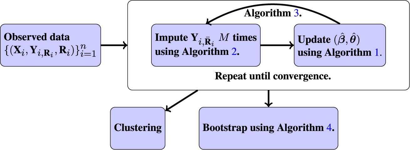
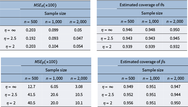


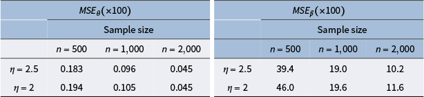


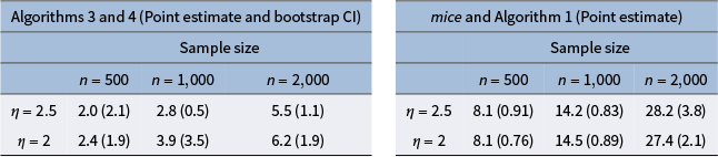
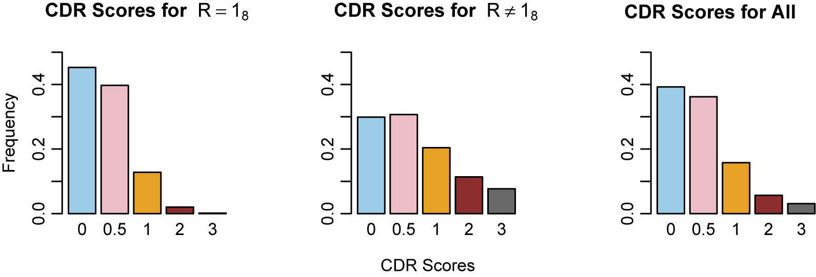
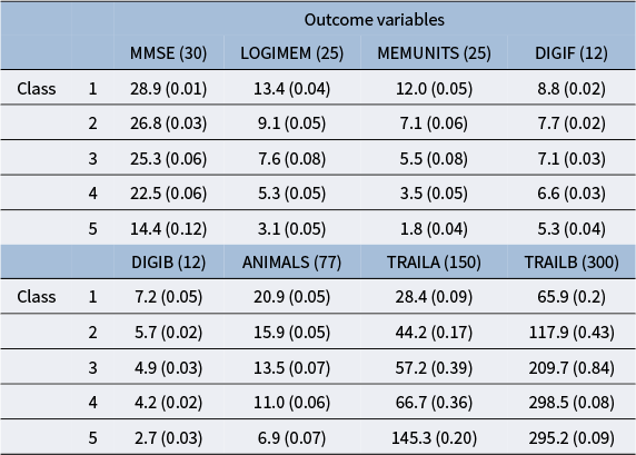
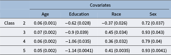
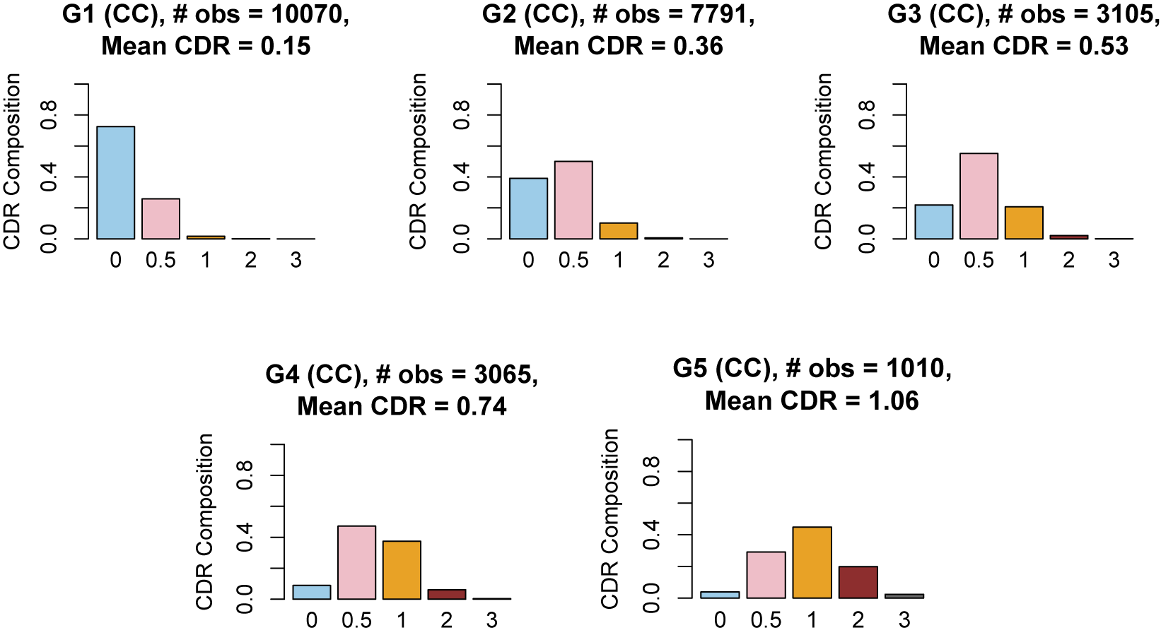
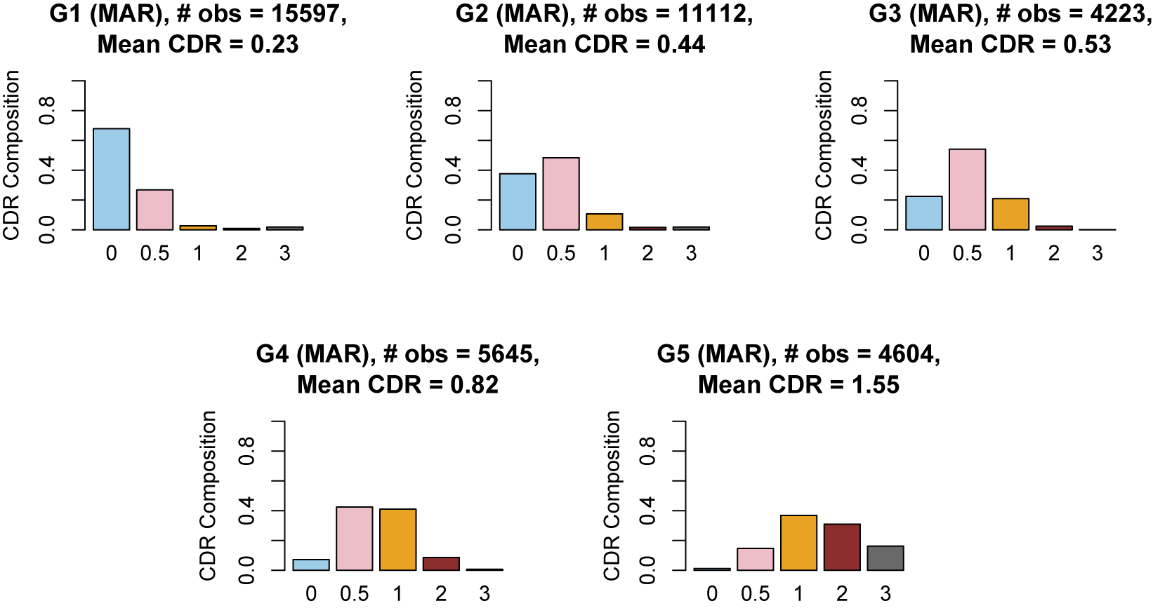


 Open access