

1. Introduction
Mass loss from the ice sheets of Greenland and Antarctica is one component contributing to sea-level rise. Between 1992 and 2011, these ice sheets lost mass equivalent to ∼11 mm of sea-level rise (Reference ShepherdShepherd and others, 2012). In the case of the Antarctic ice sheet, mass loss is dominated by the flow of ice off the continent into the floating ice shelves at the coasts. These ice shelves play a key role in determining the flow dynamics of the glaciers and ice streams that flow into them and can act to buttress the grounded ice, providing resistance to ice flow and leading to a reduced ice discharge rate. If the resistance to flow produced by the ice shelf decreases, such as when an ice shelf breaks up, there can be a dramatic increase in the speed of the glaciers and ice streams flowing into the former shelf. This phenomenon was observed following the collapse of the Larsen A ice shelf (Reference Rott, Rack, Skvarca and De AngelisRott and others, 2002) and also the collapse of the Larsen B ice shelf, where ice streams flowing into the former shelf accelerated at up to eight times their previous speed (Reference Rignot, Casassa, Gogineni, Krabill, Rivera and ThomasRignot and others, 2004) and experienced substantial thinning (Reference Scambos, Bohlander, Shuman and SkvarcaScambos and others, 2004).
There are a number of factors that may determine the magnitude (and mechanics) of the buttressing produced by the floating shelf: the ice-shelf rheology; conditions at the grounding line (e.g. ice flux and thickness); the geometry of the shelf; and the geometry of the embayment in which it is located.
Ice-shelf geometry is partially determined by the extent of the ice shelf and the calving-front position. This results from a combination of processes causing calving-front retreat, such as iceberg calving, and shelf advance due to the flow of ice at the calving front. While there has been much focus on the dynamics of calving (Reference Benn, Warren and MottramBenn and others, 2007; Reference AlleyAlley and others, 2008; Reference Bassis and JacobsBassis and Jacobs, 2013), there has been relatively little work on the flow of ice at the calving front.
Reference AlleyAlley and others (2008) proposed an empirically derived calving law, using data from ten ice shelves known to have near-stationary calving-front positions. This relationship takes the form
where c is the calving rate, w is the shelf width, is the strain-rate normal to calving front and H is the ice thickness, with all values measured at the calving front. Given that shelves with stationary calving fronts were considered, the calving rate was inferred from the ice flow speed at the calving front. Therefore, this data-derived relationship could be interpreted as a way to predict the ice flow speed at the calving front for ice shelves that retain a near-constant front position. If the relationship is written in terms of the flow speed it would take the form u ∝ w∊ H, with u being the flow speed at the calving front.
Reference AlleyAlley and others (2008) interpreted the dependence on the various parameters through consideration of how each parameter would affect the calving rate. For example, one control on calving may be the rate at which fractures open transverse to flow. It is expected that this process is strongly influenced by the rate of extension in the along-flow direction, and hence suggests a proportionality between calving rate and along-flow strain rate. In addition, it was observed from the dataset that calving rate was reduced for narrower shelves. Reference AlleyAlley and others (2008) hypothesized that this may be the result of shear with lateral boundaries causing fractures to rotate such that they are no longer aligned transverse to flow. The rotated fractures may then close up or prompt the creation of smaller icebergs.
However, if this relationship did provide insight into the calving process it also suggests an instability in the calving-front position: a small retreat would move the calving front into an area of thicker ice, with greater strain rate (once balanced with the hydrostatic pressure of the ocean), which would lead to further retreat. Alternatively, when written in terms of the flow speed at the calving front, a retreat would lead to an increase in flow speed and a readvance of the calving front.
Figure 1 (Reference AlleyAlley and others, 2008) shows data points corresponding to individual ice-shelf locations, and the linear regression used to derive the empirical relationship. The dataset used is made up of 18 data points from ten ice shelves (named in the caption to Fig. 1). A number of shelves have multiple data points corresponding to different locations on the ice shelf. The dataset is a compilation of data from numerous sources, with no apparent systematic methodology for sampling parameter values, especially with regard to along-flow strain rate.
Plot showing an empirically derived law for ice-shelf calving. Ice-shelf velocity at the calving front plotted against the product of strain rate, thickness and width for ten ice shelves: Amery (A), Filchner (F), Riiser (I1, I2), Jakobshavn (J1, J2, J3), Larsen B (L1, L2), McMurdo (M), Nivlisen (N), Ronne (O1, O2, O3), Pine Island (P) and Ross (R1, R2, R3). Adapted from Reference AlleyAlley and others (2008) and reprinted with permission from the American Association for the Advancement of Science.

A relationship for the viscous flow of ice at the calving front was derived by Reference HindmarshHindmarsh (2012) using a scaling analysis. The relationship takes the form u ∝ w(∊H)3/4. This scaling analysis is based on the physical balances and scalings that govern the viscous flow of an ice shelf as it approaches the calving front. The ice shelf is assumed to have a uniform shear-thinning rheology given by Glen’s flow law, with constant flow law parameter B and flow exponent n. The shelf is situated in a parallel channel with a no-slip condition at the lateral boundaries. Ice flows in the along-channel direction (x-direction) only, with the along-flow strain rate given by ∊ = ∂u/∂x. The channel is of width w and has a width-averaged thickness H. Despite the potential for complex ice-shelf geometry and flow upstream, flow is close to unidirectional in the region close to the calving front, which is the area of interest in this work.
The derivation of this scaling law can be summarized briefly as described below. Reference HindmarshHindmarsh (2012) provides a more detailed derivation.
The force-balance equation for the along-channel flow is given by
where g′ = g(ρ w − ρ)/ρ w is the reduced gravity. Here ρ is the density of ice, ρ w is the density of sea water and g is the acceleration due to gravity. The effective viscosity is given by
where B is the flow law parameter, eII is the second invariant of the strain-rate tensor and n is the exponent from Glen’s flow law. The second invariant is given in reduced form as there is no vertical shear within the floating shelf and flow is in the along-channel (x-direction) only.
Assuming that in the zone close to the calving front, of aspect ratio 1, the magnitude of the transverse shear stress is equal to the magnitude of the extensional stress (Reference HindmarshHindmarsh, 2012), the force-balance equation (Eqn (2)) implies that the characteristic length scale in the along-flow direction (L) scales linearly with characteristic length scale in the transverse-to-flow direction (Y)
Here the characteristic length scale transverse to flow is equal to half the channel width. At the calving front, x = xf , the extensional stress in the shelf balances the hydrostatic pressure of the ocean:
If Eqn (6) is evaluated along the centre line of the ice shelf, where ∂u/∂y = 0, it becomes
where u c is the centre-line velocity. Furthermore, by combining this with the scaling from the force-balance equation (Eqn (5)), we can derive a scaling for the velocity at the front:
This is for the case of a general Glen’s flow law rheology with flow exponent n and flow law parameter B. Assuming a constant B between ice shelves and approximating the Glen’s flow law exponent as n = 3 gives the proportionality
Reference HindmarshHindmarsh (2012) attempted to confirm this relationship using the dataset from Reference AlleyAlley and others (2008). Numerous multiple regression models were applied to the data. The four models with the highest R 2 values are presented in Table 1. From these results it is clear there is some ambiguity as to which model represents the data most accurately. Each model in Table 1 has a large R 2 value but there is little agreement between the regression parameters (when the range is disregarded). For example, the highest R 2 value (0.98) is achieved using the regression model u ∝ w(∊H) A (with A = 0.98). Similar regression model values could be obtained using the other regression models, such as the first model u ∝ w(∊H) A ; however, the resulting regression parameter for this model (A = 0.87) is substantially different.
Multiple regression models applied to the dataset from Reference AlleyAlley and others (2008) (adapted from Reference HindmarshHindmarsh, 2012)
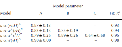
This ambiguity may be due to the relatively small number of shelves used in the analysis (18 data points from ten ice shelves), or the fact that some data points were from locations away from centre lines. In addition, the data points corresponding to Jakobshavn and Pine Island Glacier (PIG) have very high speed values in comparison with the other ice shelves in the dataset. It is reasonable to suggest that these shelves have experienced large-scale damage, leading to a reduced effective ice viscosity and therefore a decrease in the resistance provided to the ice-shelf flow; consequently they achieve much greater flow speeds.
In order to clarify the previous work of Reference AlleyAlley and others (2008) and Reference HindmarshHindmarsh (2012) and determine a relationship for the flow at the calving front, it is necessary to compile a large dataset using a systematic method to determine values for shelf width, thickness, speed and strain rate. The details of this process are given in Section 2, where data are collected from 22 Antarctic ice shelves ranging in size and aspect ratio, and not limited to shelves with near-stationary calving-front positions. Values are sampled systematically at points corresponding to central calving-front locations. In Section 3 the newly compiled dataset is analysed to determine a relationship for ice flow speed at the calving front. An initial assessment of the data is undertaken using a robust regression procedure applied iteratively to the dataset (see Section 3 for details) before the ice shelves are classified depending on their geophysical characteristics in order to establish a suitable regression for the dataset. In doing this we identify a relationship for flow speed at the calving front for laterally confined ice shelves with close to uniform rheological parameters.
2. Data Collection/Compilation
Data were compiled for 22 Antarctic ice shelves, ranging in size from the large Ross and Ronne ice shelves to the smaller Cook and Dolleman (Las Heras) Glacier ice shelves. Data for ice-shelf thickness were obtained from the Bedmap2 dataset (Reference FretwellFretwell and others, 2013), which provides ice thickness measurements on a 1 km grid. Ice-shelf widths were taken from the Moderate Resolution Imaging Spectroradiometer (MODIS) Mosaic of Antarctica (MOA) image map (Reference Haran, Bohlander, Scambos, Painter and FahnestockHaran and others, 2005), with values measured using the software ArcGIS. Here the shelf width is defined as the straight-line distance between the final two lateral pinning points, which are identified from the MOA grounding line and coastline outlines. This shelf width definition is used for all shelves, even when the shelf protrudes past the final pinning points.
2.1. Ice-shelf speed and strain rate
Measurements of ice speed and strain rate at the calving front were obtained using the dataset of Reference Rignot, Mouginot and ScheuchlRignot and others (2011a). The updated version of the dataset provides velocity measurements on a 450 m grid for the whole of Antarctica (Reference Rignot, Mouginot and ScheuchlRignot and others, 2011b). This dataset is a compilation of interferometric synthetic aperture radar (InSAR) data collected between 2007 and 2009. Owing to numerous datasets spanning the time period in some regions and fewer datasets in others, there is some spatial and temporal variability in the data. There are also errors arising from data processing. Error values for the velocity data are provided as part of the published data product and can be seen for the Amery Ice Shelf in Figure 2b. It is possible to identify clear banded regions in the error values, which may represent boundaries between satellite swath patches. In order to obtain values of strain rate, a spatial derivative of the velocity field must be taken. In doing so, the boundaries between error regions will become prominent. This issue is addressed and sharp variations are smoothed by applying a low-pass Gaussian filter. The filter uses data from an area of 40 × 40 gridcells (18 km × 18 km) centred on the target cell, with a standard deviation (SD) of four gridcells (1.8 km). This smoothed velocity field is used to give the ice flow speed at the calving front and also the inferred strain rate. These parameter values for the Gaussian filter are chosen to preserve the large-scale features in the strain-rate field, but to remove small-scale artefacts present from data collection processes. From visual assessment these parameter values provide an appropriate strain-rate field and can be compared with the strain-rate field generated by other parameter choices (see Fig. 10 below in the Appendix).
Plots for the Amery Ice Shelf: (a) unfiltered velocity field (m a−1) from Reference Rignot, Mouginot and ScheuchlRignot and others (2011b); (b) velocity field error values (m a−1) from Reference Rignot, Mouginot and ScheuchlRignot and others (2011b); (c) strain-rate field (a−1) calculated from unfiltered velocity field; (d) strain-rate field (a−1) calculated from filtered velocity field using low-pass Gaussian filter (range 18 km × 18 km, SD 1.8 km). The large negative values at the calving front (blue) are an artefact of applying the low-pass filter to the velocity field; valid strain-rate values begin 9 km back from the original calving front. Plots include grounding line outline and coast outline from MOA (Reference Haran, Bohlander, Scambos, Painter and FahnestockHaran and others, 2005).

The filtered velocity field is used to calculate the two-dimensional (2-D) strain-rate tensor

Values of the strain-rate tensor are calculated at each point in the velocity field using a shifted grid, with shifted-grid values obtained by averaging the velocity values over the surrounding points, as shown in Figure 3.
Schematic for calculating strain-rate tensor. Grid and data points for the original 450 m velocity dataset are shown as solid lines and points. The shifted grid used to calculate the strain rate at point X is depicted using dashed lines and grey points. Velocities are calculated at points A, B, C and D from the mean of four surrounding original data points. The strain rate at X is determined by averaging appropriate velocity differences between points A, B, C and D.

In this work, the strain rate is defined as the along-flow strain rate and gives a measure of the strain in the direction of flow at each point. It is given in vector notation as
![]() , where
, where
![]() is the unit vector in the flow direction. This along-flow strain rate is calculated for all grounded and floating ice. It is assumed that the flow at the calving front is perpendicular to the calving face; therefore, the strain rate in the direction of flow should be equivalent to the strain rate normal to the calving front. After visual assessment of the angle at which the streamlines meet the calving front, it is clear that this assumption is broadly true. The speed and the non-filtered and filtered strain-rate fields for the Amery Ice Shelf are shown in Figure 2a, c and d, respectively. From Figure 2c and d it is clear that the filtered velocity field provides a much smoother strain-rate field in comparison with the unfiltered data; however, the detail of large-scale features is still visible, such as increased positive extensional strain values in the shelf following the input of ice from the ice stream on the west side of the Amery Ice Shelf. An artefact resulting from this filtering process is the presence of large negative values of strain at the boundary with the ocean. These values are not representative of strain rates close to the calving front, with valid strain rates beginning 9 km back from the original calving front.
is the unit vector in the flow direction. This along-flow strain rate is calculated for all grounded and floating ice. It is assumed that the flow at the calving front is perpendicular to the calving face; therefore, the strain rate in the direction of flow should be equivalent to the strain rate normal to the calving front. After visual assessment of the angle at which the streamlines meet the calving front, it is clear that this assumption is broadly true. The speed and the non-filtered and filtered strain-rate fields for the Amery Ice Shelf are shown in Figure 2a, c and d, respectively. From Figure 2c and d it is clear that the filtered velocity field provides a much smoother strain-rate field in comparison with the unfiltered data; however, the detail of large-scale features is still visible, such as increased positive extensional strain values in the shelf following the input of ice from the ice stream on the west side of the Amery Ice Shelf. An artefact resulting from this filtering process is the presence of large negative values of strain at the boundary with the ocean. These values are not representative of strain rates close to the calving front, with valid strain rates beginning 9 km back from the original calving front.
2.2. Representative values for strain rate, speed and thickness
For each ice shelf, a series of 20 flowlines spaced about the approximate centre of the shelf trace the path taken by ice as it flows from the main body of the shelf towards the calving front. Along these flowlines, values of thickness, speed and strain rate can be sampled. In the scaling analysis of Reference HindmarshHindmarsh (2012), equations were evaluated along the centre line of the ice shelf. In order to extract comparative values from the data, the flowline with maximum speed at the calving front is determined and then values are sampled along it. Theoretically, the maximum speed should be achieved on the centre line at the calving front.
The strain-rate field for the Getz Ice Shelf along with the flowline of maximum velocity can be seen in Figure 4a. Strain-rate values extracted along the maximum speed flowline are shown in Figure 4b and c. From these plots it is clear that despite the smoothing effect of the Gaussian filter there is still a large range of strain-rate values as the ice approaches the calving front. This range in strain rate can also be observed in the plan-view plot of strain rate (Fig. 4a), where there is spatial variability in the strain-rate value. This may be a feature of the ice flow or the result of ice damage (crevassing), which may lead to a reduced effective viscosity of the ice and corresponding high strain values. Alternatively, the high spatial variability may be due to errors in the velocity field.
The process of calculating strain rate at the calving front of the Getz Ice Shelf. (a) Along-flow strain rate (a−1), with flowline of maximum velocity along which values of strain rate, speed and thickness are sampled. The large negative values at the calving front are an artefact of applying the low-pass filter to the velocity field; valid strain-rate values begin 9 km back from the original calving front. (b) Values of strain rate (a−1) (blue curve) and speed (m a−1) (orange curve) along flowline of maximum velocity. Bold green line indicates mean strain rate over final 20 km. (c) Values of strain rate (a−1) (blue crosses) sampled along final 20 km of maximum velocity flowline, with mean strain rate (bold green line) and SD (dashed red line).

To determine a representative strain rate systematically for the range of ice shelves used in this study, the mean strain rate over the final 20 km of the maximum speed flowline is used (exceptions: McMurdo Ice Shelf for which the mean was calculated over the final 10 km due to a gap in the data; and Publications Ice Shelf for which the mean was calculated over the final 15 km as it is a small shelf). For all shelves, apart from the Robert Glacier and the Venable ice shelves, 20 km is less than half the width of the shelf (see Table 3 below in Appendix for shelf-width details). This suggests that the mean strain rate may be representative of the strain rate in the frontal region of the shelf. Here we aim to clarify the large-scale dynamics and test the scaling argument of Reference HindmarshHindmarsh (2012); therefore, it is necessary to use values that are representative of the large-scale dynamics.
The 20 km section begins 9 km back along the flowline from the original calving front, to account for the 9 km range of the Gaussian filter. Values of ice thickness and speed are also collected on the maximum speed flowline at this newly defined calving-front position. The process of calculating the mean strain rate is shown in Figure 4a, b and c for the Getz Ice Shelf. The mean strain-rate value (bold green curve) is shown in Figure 4b in relation to the values along the maximum velocity flowline, while in Figure 4c the final 20 km section is shown in detail. The mean strain rate for the Getz Ice Shelf is calculated to be 0.01 a−1, with a SD of 0.005 a−1; most strain values along this 20 km transect are included within one SD of the mean, with the exception being some higher values at the downstream end of the section.
The process of sampling ice thickness, speed and strain rate at the centre of the ice-shelf calving front is repeated for 22 Antarctic ice shelves and paired with data for the ice-shelf width. (Table 3 in the Appendix lists all the data compiled.) Plots for all 22 ice shelves used to compile the dataset, such as those from the Getz Ice Shelf in Figure 4, can be found in the supplementary material available at http://www.igsoc.org/hyperlink/15j116_supp.pdf.
3. Data Analysis
From the work of Reference AlleyAlley and others (2008) and Reference HindmarshHindmarsh (2012), we expect a relationship of the form u = Aw(∊H) B (with B = 1 in the case of Reference AlleyAlley and others (2008) and B = 3/4 in the case of Reference HindmarshHindmarsh (2012)) to relate the variables at the ice-shelf calving front. A relationship of either form should produce a linear trend in log–log space. Data from the 22 Antarctic ice shelves are plotted in log–log space in Figure 5. From this plot we can see that there is a broadly positive correlation between the variables u/w and ∊H. However, there is a large degree of scatter in the data. Visual assessment suggests that the PIG, Fimbul and Dolleman ice shelves may be outliers.
Full dataset of 22 Antarctic ice shelves, plotting speed divided by shelf width (u/w) against strain rate multiplied by shelf thickness (∊H) in log–log space. Vertical error bars (green) denote SD in speed from mean speed, plotted about point measurement of speed. Horizontal error bars (dashed blue) denote SD in strain rate.

Figure 5 also shows error values associated with the data points, with u/w plotted against ∊H in log–log space. Mean values of strain rate are calculated over the final 20 km of the shelf, while point measurements of speed are used. Horizontal error bars indicate the SD ( σ) in the strain rate (strain rate calculated from filtered velocity field) over the final 20 km of each shelf (log((∊ − σ)H) to log((∊ + σ)H)). Vertical error bars give the SD in speed over the same 20 km transect, away from the mean speed value. This mean speed value is calculated and given in Table 3 in the Appendix, but not shown in Figure 5. However, when plotted, the mean values are located very close to the point measurement values. From the plot in Figure 5 it is evident that the SD in speed is small, which suggests confidence in the accuracy of the speed values. When comparing the SD in speed calculated here with the error in flow speed provided as part of the original data product (Reference Rignot, Mouginot and ScheuchlRignot and others, 2011a; see Table 3 in the Appendix for details) we see that the SD is of the same order of magnitude or higher, indicating that the original errors in the velocity field are not significant for this analysis.
The SD in strain rate is much larger, which is expected given the high spatial variability in strain rate observed in Section 2. Values with large strain rate appear to have smaller SDs, but this may be because data points with low strain-rate values have large relative SDs. From Figure 5 it is clear that there is a large degree of scatter in the data and some uncertainty in the horizontal position of data points.
As part of an initial assessment we apply a robust regression procedure iteratively to the full dataset, with the aim of identifying a linear trend in log–log space. A robust regression is similar to a least-squares regression but with data points reweighted depending on the size of their residual until an optimum regression model is achieved. Here we use the MATLAB® robust fitting option for a linear regression model with a bisquare weight function. The robust regression procedure is outlined by Reference Holland and WelschHolland and Welsch (1977). Using this method the most outlying data point can be identified and removed from the dataset. If this process is repeated, more outlying data points can be identified and removed until a threshold R 2 value is achieved, indicating that a regression model has been obtained with a good fit to the data. We choose a threshold R 2 value of 0.8, which is exceeded for this dataset once nine ice-shelf data points have been removed. The regression model takes the form log(u/w) = A + Blog(∊H), with slope B = 0.64 and R 2 = 0.83 (see Fig. 11 in the Appendix). Here all outliers are positioned above the regression line, suggesting a fundamental difference between the outlying and included ice shelves. Although this procedure allows a linear trend to be identified in log–log space, there is no physical premise or understanding used to determine which shelves are removed.
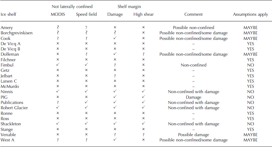
In the scaling analysis of Reference HindmarshHindmarsh (2012), two assumptions were made in order to obtain the scaling relationship. First it was assumed that the shelf was laterally confined between pinning points. Secondly, the ice shelf was assumed to conform to a Glen’s flow law rheology, with constant flow law parameters B and n. This ensures comparable rheology in the ice-shelf margins and along the centre line of the shelf. Preliminary assessment of the ice shelves in this dataset shows that some are not laterally confined at the calving front and there are some that may have non-uniform ice rheology. We therefore look to make a classification of the geophysical characteristics of the shelves in relation to their confinement and rheology.
3.1. Classification of the geophysical characteristics of ice shelves
Assessment of ice-shelf confinement is undertaken using visual MODIS data and plots of the surface velocity field to identify whether the calving front is laterally confined. We define the calving front to be laterally confined if a section of the ice shelf less than half the shelf width protrudes into the open ocean past the final pinning point. The MODIS data are used to identify the extent of the shelf, while the velocity field can be utilized to locate pinning points and stationary ice along the ice-shelf margins.
The second assumption, concerning uniform ice-shelf rheology, is addressed through analysis of MODIS imagery to identify the presence of ice damage in the form of fractures and crevasses, which may lead to a reduction in the effective ice viscosity. In addition, the transverse shear field (
![]() , with
, with
![]() the unit vector normal to flow direction) is calculated to determine whether a threshold transverse shear value is exceeded in the margins of the shelf. We use a threshold value of 0.05 a−1.
the unit vector normal to flow direction) is calculated to determine whether a threshold transverse shear value is exceeded in the margins of the shelf. We use a threshold value of 0.05 a−1.
This threshold strain-rate value corresponds to a shear stress of 130 kPa, assuming a Glen’s flow law rheology as in Eqn (3), with n = 3 and B = 2.84 × 10⁸ s1/3 Pa (B value at −10°C from Reference Cuffey and PatersonCuffey and Paterson (2010), and approximating the second invariant of the strain-rate tensor with the transverse shear value divided by 2
![]() . This shear stress is greater than the 70 kPa critical stress value used by Reference Albrecht and LevermannAlbrecht and Levermann (2012) when simulating the evolution of fractures on the Ronne and Filchner ice shelves. However, it sits within the estimates for maximum stress derived from field measurements, which give values of 90–320 kPa (Reference VaughanVaughan, 1993). Comparisons can also be made with values of basal shear stresses for grounded ice, which rarely exceed 70 kPa over large areas (Reference Joughin, MacAyeal and TulaczykJoughin and others, 2004).
. This shear stress is greater than the 70 kPa critical stress value used by Reference Albrecht and LevermannAlbrecht and Levermann (2012) when simulating the evolution of fractures on the Ronne and Filchner ice shelves. However, it sits within the estimates for maximum stress derived from field measurements, which give values of 90–320 kPa (Reference VaughanVaughan, 1993). Comparisons can also be made with values of basal shear stresses for grounded ice, which rarely exceed 70 kPa over large areas (Reference Joughin, MacAyeal and TulaczykJoughin and others, 2004).
Where regions of high shear rate are identified using the 0.05 a−1 threshold, there are often sites of higher shear rate contained within these regions. Therefore this critical shear stress represents a minimum stress in these areas and it is likely that there are locations where the shear stress is higher. Including the other two components of the strain-rate tensor, the along-flow and perpendicular-to-flow strain, in the calculation of the second invariant will also contribute to increasing the value of shear stress. This suggests these areas of high shear rate (>0.05 a−1) correspond to regions where fractures and crevasses form. Once this damage has occurred, the ice can no longer be described using constant flow-law parameters (B and n in Glen’s flow law) and therefore the Reference HindmarshHindmarsh (2012) scaling relation breaks down.
The links between weak ice, damage (crevasses and fractures) and areas of high shear were considered in the work of Reference SandhägerSandhäger (2003) and Reference Vieli, Payne, Du and ShepherdVieli and others (2006) when reconstructing the flow field for the pre-collapse Larsen B ice shelf. Reference SandhägerSandhäger (2003) compared an ice-shelf model with uniform rheological parameters with one adjusted to account for weak viscosity in areas of high shear stress and areas with ice advected from areas of high shear. In doing so, it was observed that the adjusted model more accurately reproduced the flow field. This mechanical effect was attributed to ice damage in the form of fractures and crevasses sustained after undergoing high shear. High shear areas were identified by determining whether the modelled shear stress had exceeded a critical value. Reference Vieli, Payne, Du and ShepherdVieli and others (2006) hypothesized that high shear could lead to heating and weakening of the ice, while the formation of crevasses would allow surface melt to penetrate more deeply and warm the ice in these regions, leading to further softening. Reference Vieli, Payne, Du and ShepherdVieli and others (2006) identified weak ice margins as playing a dominant role in controlling the flow of the Larsen B ice shelf and were able to locate weak ice zones by inverting for the flow law parameter B. This technique provided a better fit to observations than a model with uniform B.
Using the criteria for lateral confinement and weak ice margins, each shelf is allocated to one of three groups: YES – ice shelves that conform to the assumptions of the scaling analysis being laterally confined with uniform rheology; NO – ice shelves that are not laterally confined and/or have non-uniform rheology; MAYBE – shelves for which it is unclear whether the assumptions are valid.
3.1.1. Examples of geophysical characteristics and classification
Here we show two examples of the geophysical classification of ice shelves, depending on their lateral confinement and rheology. (Plots used for the geophysical classification of all shelves can be found in the supplementary material at http://www.igsoc.org/hyperlink/15j116_supp.pdf) Plots for the Fimbul Ice Shelf are shown in Figure 6a (MODIS imagery), b (velocity field), c (strain-rate field) and d (shear-rate field). From visual assessment of the MODIS image (Fig. 6a), it is clear that the calving front is not laterally confined, with a large section of the shelf, approximately one shelf-width long, protruding out past the pinning points. The velocity field (Fig. 6b) shows high values of ∼700 m a−1 in the main body of the ice shelf, but slow-moving sections of ice (possibly grounded) are observed further upstream prior to the unconfined section. It is clear that the calving front has moved past these pinning points to form an ice tongue. The MODIS image shows some fracturing along the left margin of the shelf, which appears to correspond with high positive along-flow strain (Fig. 6c) rather than high transverse shear (Fig. 6d).
Plots for the Fimbul Ice Shelf: (a) MODIS image; (b) velocity field (m a−1); (c) along-flow strain-rate field (a−1) with maximum velocity flowline; (d) transverse shear rate (a−1). Note that artefacts due to the filtering of the velocity field are present near the ice–ocean boundary for the along-flow strain and transverse shear rates. All plots include grounding line, islands and coast outline. This is an example of a NO ice shelf as the calving front has passed the final lateral pinning points.

Figure 7a–d show MODIS imagery, velocity field, strain-rate field and shear-rate field for the PIG ice shelf. From the MODIS (Fig. 7a) and velocity field (Fig. 7b) plots it is clear that the ice shelf is confined laterally between sections of slow-moving ice. However, from the MODIS data it is evident that there is a large amount of crevassing and fracturing in the ice shelf. Assessment of the velocity field indicates a large gradient in speed between the main body of the ice shelf, flowing at >3500 m a−1, and the near-stationary margins. This feature is clearly evident in the plot of transverse shear rate (Fig. 7d), where high values of shear are observed in the shelf margins, saturating the colourscale, which is limited by the 0.05 a−1 threshold criterion for uniform rheology. It is also clear that the margins and grounding line of the shelf are areas of high positive strain rate (Fig. 7c). Based on the presence of numerous fractures and the high shear values in the shelf margins, we classify the PIG ice shelf as having weak margins.
Plots for the PIG ice shelf: (a) MODIS image; (b) velocity field (m a−1); (c) along-flow strain-rate field (a−1) with maximum velocity flowline; (d) transverse shear rate (a−1). Note that artefacts due to the filtering of the velocity field are present near the ice–ocean boundary for the along-flow strain and transverse shear rates. All plots include grounding line, islands and coast outline. This is an example of a NO ice shelf due to the high shear values exceeding 0.05 a−1 in the shelf margins.

Table 2 lists all 22 ice shelves, their geophysical characteristics and their classification.
Classification of ice shelves in terms of the lateral confinement of the calving front and the presence of damage in ice-shelf margins or high shear values (≥0.05 a−1) in margins
3.2. Analysis of laterally confined and uniform rheology shelves
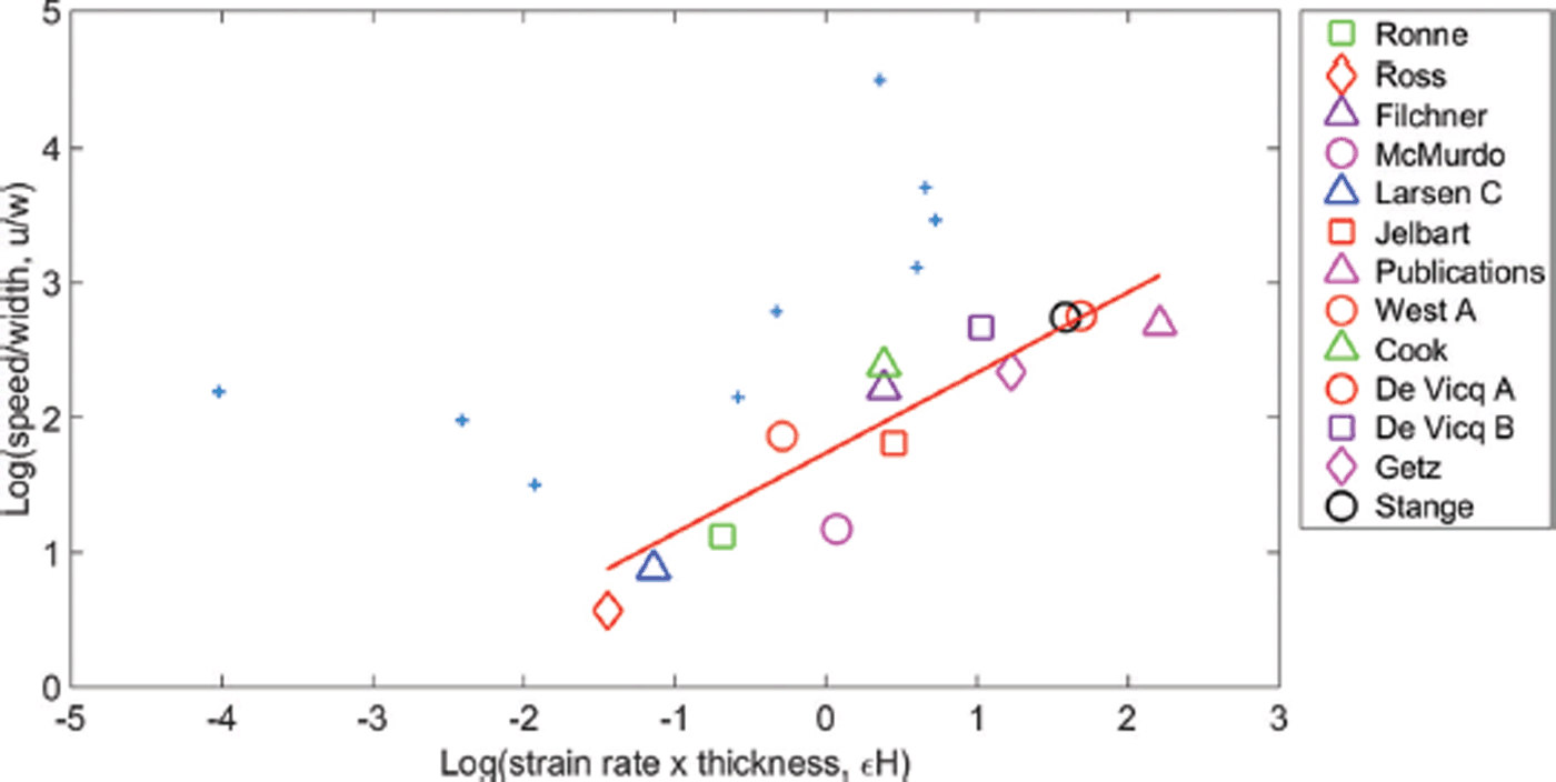
Using the geophysical classification, we now investigate relationships between the variables for the YES category of ice shelves, i.e. those that are laterally confined and have uniform rheological parameters. Data from this subgroup of ten ice shelves are plotted in log–log space in Figure 8. A least-squares linear regression is then applied to the data, which produces a model of the form log(u/w) = 1.60 + 0.72 log(∊H), with an R 2 value of 0.92. The linear fit can be seen in Figure 8, which includes the 95% confidence interval for the regression along with the excluded data points from the full dataset. This linear regression suggests the proportionality u ∝ w(∊H)0.72, which is close to the relationship Reference HindmarshHindmarsh (2012) derived from the scaling analysis (u ∝ w(∊H)0.75).
Scatter plot of u/w against ∊H in log–log space. Shelves that are laterally confined and have close to uniform rheological parameters are identified in the key, with a least-squares linear regression applied to the data (red line). The blue dashed curves bound the 95% confidence interval for this regression model. Data points from the full dataset that are not included in the regression are denoted by purple crosses.

The regression model can also be plotted in linear space (Fig. 9). Here we observe that the regression model provides a good fit to the data. A number of points are clustered close to the origin, but using a regression in log–log space enables the nonlinear trend through these points to be clearly identified. Again the data points for the excluded ice shelves are included in this plot and it is clear that they mostly lie above the curve, indicating that the speed at the calving front for the excluded shelves is greater than expected for the laterally confined shelves. This is probably a consequence of the reduced resistance to flow due to the absence of lateral pinning points or the presence of weak/damaged margins.
Scatter plot of u/w against ∊H. Least-squares regression model calculated in log–log space but plotted here in linear space (red curve). Data points excluded from the regression model due to non-lateral confinement and/or weak margins are denoted by purple crosses. Two excluded data points are outside the field of view: PIG at (1.45, 90.4) and Publications at (9.1, 14.8).

4. Discussion and Conclusions
We have aimed to build on and clarify the work of Reference AlleyAlley and others (2008) and Reference HindmarshHindmarsh (2012) concerning the ice flow dynamics in the zone close to the ice-shelf calving front, primarily by compiling a larger dataset to compare with a relationship derived from a scaling analysis. From this dataset of 22 Antarctic ice shelves, we have observed that there is a positive correlation between the speed of ice at the calving front and the product of shelf width, strain rate and ice thickness. However, there is a large degree of scatter to the data when looking for trends.
In the process of analysing the data we have identified a subgroup containing those ice shelves that are laterally confined and have close to uniform rheological parameters. Applying a least-squares regression model to this data gives the proportionality u ∝ w(∊H)0.72, with an R 2 value of 0.92. This is close to the scaling analysis relationship derived by Reference HindmarshHindmarsh (2012), u ∝ w(∊H)3/4. Possible explanations for this variance are: small spatial variations in rheological parameters (B and n) not considered in the scaling analysis; the Glen flow exponent n may differ slightly from 3; non-parallel lateral boundaries at the calving front, allowing extension laterally; asymmetric or varying ice flux from upstream; effects of submarine melting or freeze-on; and errors in the data and data compilation.
When comparing laterally confined and non-damaged ice shelves with the remaining shelves in the dataset it is clear that the remaining shelves have greater ice flow speeds at the calving front. This may be explained by the reduced resistance to flow these shelves experience due to the absence of lateral pinning points or weak rheology in the shelf margins.
It is clear that the spatial variation in flow law parameters plays an important role in controlling the flow dynamics of the ice shelf. Additional features pertaining to ice rheology that could be considered in future theoretical assessments of ice flow at the calving front include: spatially varying rheological parameters such as the flow law parameter B and the Glen flow exponent n; spatially varying the ice temperature field; or considering the ice deformation history (strain and shear history). A more thorough assessment of the spatial variation in ice-shelf rheological parameters could be undertaken by inverting for the rate factor. This would allow a quantitative measure of weakening in the ice-shelf margins to be used when making a geophysical classification of the ice shelves.
For some shelves in the NO and MAYBE groups, the effective ice rheology appears to be close to uniform (undamaged); however, data from these shelves cannot be compared with the scaling relation because the calving front is located on ice that protrudes past the final lateral pinning points. Additional data could be included from these shelves by taking values of speed, strain rate, ice thickness and width at the final pinning point of the shelf. This would only be valid for shelves where the final pinning points form a parallel section of the channel. Once ice flows past this final pinning point the ice tongue section of the shelf theoretically exerts no buttressing on the confined shelf. Therefore the dynamics at the pinning point should remain the same regardless of the presence of the ice tongue. This location could be determined by constructing a straight line between the two final lateral pinning points and finding where this line intersects the flowline of maximum velocity. Alternatively, the principal axes of strain could be calculated. The second principal axis of strain could then be used to determine where there is a transition from negative (upstream and confined) to positive (downstream and unconfined) strain values. This transition from negative second principal strain to positive second principal strain should define where the ice has started to spread laterally as it leaves the confines of pinning points.
Comparing the dataset presented in this paper with the dataset of Reference AlleyAlley and others (2008), we see that for most of the ice shelves included in both datasets (Amery, Filchner, Ronne and Ross) the data are consistent (exceptions are the McMurdo and PIG ice shelves). Ice-shelf data points from Reference AlleyAlley and others (2008) plotted alongside this new dataset occur on or above the regression line we determine after geophysical interpretation.
The empirical law derived by Reference AlleyAlley and others (2008) was designed to be descriptive of calving. Although the work presented in this paper is not informative of calving, the newly compiled dataset gives values of strain rate close to the calving front and could suggest a criterion for critical strain rates that can be sustained for ice shelves with a certain flow speed, thickness and width. By inverting the plots of u/w against ∊H, it is clear that the regression curve provides an upper bound on the product of strain rate and thickness for the range of shelves. This bounding curve was found using the mean strain rate over the final 20 km of the shelves, so it is expected that higher strain rates would be plotted if the maximum strain rate along the flowline were considered, therefore increasing the values of this bounding curve. For the non-confined shelves, values of shear and transverse strain, in addition to along-flow strain, may be informative of the deformation occurring at the calving front. These values may be useful in determining the material properties of ice at the calving front and helpful for predicting calving events.
From this investigation we have determined that the scaling analysis of Reference HindmarshHindmarsh (2012) agrees well with the data collected for ice shelves that are laterally confined and have close to uniform rheological parameters. However, this scaling breaks down when the shelves are no longer confined and are able to spread in both the along-flow and transverse-to-flow directions, or when weak ice in the shelf margins results in reduced resistance to flow.
5. Data Statement
All data used in this work are listed in Table 3 or can be found in the supplementary material: http://www.igsoc.org/hyperlink/15j116_supp.pdf.
Acknowledgements
This work was supported by a British Antarctic Survey studentship funded by the Natural Environment Research Council, grant No. NE/K50094X/1. We are grateful for the support and useful comments of Robert Arthern and Hilmar Gudmundsson.
Appendix
The strain-rate field resulting from the application of different low-pass Gaussian filters to the velocity field, with filter ranges 9, 18 and 36 km and SDs 0.9, 1.8 and 3.6 km, are shown in Figure 10. Here it is clear that the 18 km filter smooths small-scale artefacts but retains the larger-scale strain-rate pattern.
Plots for the Amery Ice Shelf: (a) along-flow strain rate (a−1) calculated from unfiltered velocity field; (b–d) along-flow strain rate (a−1) calculated using Gaussian low-pass filter applied to velocity field, with range (b) 9, (c) 18 and (d) 36 km and SD (b) 0.9, (c) 1.8 and (d) 3.6 km. All plots include grounding line outline and coast outline from MOA (Haran and others, 2005).

Linear regression achieved after removing nine outlying data points using an iterative robust regression process. Removed points shown as blue crosses.
Full dataset for 22 Antarctic ice shelves

The results of the robust regression procedure applied iteratively to the full dataset can be seen in Figure 11. Here an R 2 value of 0.83 is achieved once nine ice shelves have been removed from the initial dataset. The resulting regression model takes the form log(u/w) = A + B log(∊H), with intercept A = 1.67 and slope B = 0.64.
The full dataset used in this work is given in Table 3, with values for shelf width, shelf thickness, flow speed, strain rate, mean speed over final 20 km section, standard deviation (SD) in strain rate and speed, and error in velocity field from Rignot and others (2011a).


