


1. INTRODUCTION
Global mean sea-level rise (SLR) threatens coastal and island populations worldwide, but large uncertainties remain in near-term projections of the threat (e.g. Church and others, Reference Church, Stocker, Qin, Plattner, Tignor, Allen, Boschung, Nauels, Xia, Bex and Midgley2013; Horton and others, Reference Horton, Little, Gornitz, Bader and Oppenheimer2015). Ice sheets and glaciers provide the largest—and most uncertain—contribution to projected 21st century SLR (Church and others, Reference Church, Stocker, Qin, Plattner, Tignor, Allen, Boschung, Nauels, Xia, Bex and Midgley2013), with integrated mass loss from Greenland, Antarctica and the large number of smaller glaciers worldwide each responsible for about one third of the sea-level contribution observed at present (Gardner and others, Reference Gardner2013). The Greenland ice sheet sheds mass to the ocean through a drainage network of tidewater glaciers, and the sea-level contribution from Alaska glaciers is especially large (Larsen and others, Reference Larsen2015). Tidewater glaciers such as Alaska's Columbia Glacier are susceptible to instability that can drive rapid retreat and loss of ice mass to the ocean. Thus, improving understanding of tidewater glacier dynamics is crucial to decreasing uncertainty in SLR projections. This is especially important given that about half of recently observed acceleration of Greenland mass loss is attributed to dynamic discharge of solid ice to the ocean through iceberg calving (Straneo and others, Reference Straneo2013), a mechanism that also dominates mass loss from Alaska tidewater glaciers (O'Neel and others, Reference O'Neel, Echelmeyer and Motyka2003; Larsen and others, Reference Larsen, Motyka, Arendt, Echelmeyer and Geissler2007; McNabb and others, Reference McNabb2012).
Despite the dominant role iceberg calving plays in current and projected mass loss from ice sheets and glaciers, calving remains poorly understood. Part of the difficulty in understanding stems from the large number of factors influencing calving (e.g. local meteorology, ocean temperature and circulation, glacier geometry) for which available data are limited (Benn and others, Reference Benn, Warren and Mottram2007; Straneo and others, Reference Straneo2013). Even when data are available, observations show contradictory behavior for glaciers in different environments. For example, Alaskan tidewater glaciers very rarely form floating ice tongues, but when they do (as in the case of Columbia Glacier in later stages of its ongoing retreat) they may show more large-scale and fewer small-scale calving events (Walter and others, Reference Walter2010; Bassis and Jacobs, Reference Bassis and Jacobs2013). This suggests another challenge to understanding calving: the wide variety of spatial and temporal scales involved. Different styles of iceberg calving may be observed at sub-hourly, multi-weekly and decadal timescales (Amundson and Truffer, Reference Amundson and Truffer2010; Bassis and Jacobs, Reference Bassis and Jacobs2013). Further, the calving contribution from small glaciers is difficult to capture at the model resolutions typical of continental-scale ice-sheet models (e.g. Bassis, Reference Bassis2011).
Current ice-sheet models treat glacier ice as a viscous fluid, without a physically-consistent method for simulating iceberg calving. Several parameterizations for calving are used, varying in complexity according to the intended application of the model. One relatively simple approach treats calving rate and/or the calving fraction of total ice loss as a directly adjustable parameter (e.g. Price and others, Reference Price2015). Another approach requires ice to calve from an ice-sheet margin when it thins below a given thickness; the threshold ice thickness can be constrained by observations, such as the 150 m minimum ice shelf thickness observed in present-day Antarctica (Peyaud and others, Reference Peyaud, Ritz and Krinner2007).
Recently, more continuum-based calving criteria have begun to be implemented in ice-sheet models. One such approach is damage mechanics, which introduces ice ‘damage’ from fracturing as a state variable that affects ice flow (Pralong and Funk, Reference Pralong and Funk2005; Borstad and others, Reference Borstad2012; Duddu and others, Reference Duddu, Bassis and Waisman2013). Calving can be set to occur once damage reduces the load-bearing capacity of the ice by a certain percentage, constrained by analysis of large calving events such as the Larsen B ice shelf collapse (Borstad and others, Reference Borstad2012). Significant controversy remains, however, about how to formulate the damage evolution law. A related approach ties calving to penetration of surface and basal crevasses. This crevasse-depth criterion assumes that glacier ice calves off once surface crevasses reach the waterline or surface and basal crevasses connect, and further that the calved ice immediately ceases to interact with the rest of the glacier (Benn and others, Reference Benn, Warren and Mottram2007; Nick and others, Reference Nick, van der Veen, Vieli and Benn2010; Bassis and Walker, Reference Bassis and Walker2012). These models, however, typically require the addition of surface meltwater into crevasses to trigger calving and treat meltwater as a parameter that is adjusted to approximate observations (as in Nick and others, Reference Nick, van der Veen, Vieli and Benn2010). Newer methods, based on discrete particles (e.g. Åström and others, Reference Åström2013; Bassis and Jacobs, Reference Bassis and Jacobs2013) or self-organized criticality of glacier termini (Astrom and others, Reference Astrom2014) are promising, but too computationally expensive to be routinely used in prognostic ice-sheet models.
Here we propose a different approach that integrates some of the advantages of particle-based methods and continuum-based methods, but which is much simpler than previously proposed approaches. We assume that above a yield strength, fractured glacier ice deforms much more rapidly than intact glacier ice. Because the flow of ice is rapid above the yield strength, the yield strength provides an upper bound on the state of stress within the glacier. Assuming that the glacier is everywhere near this critical state of stress corresponds to the perfect plastic approximation, first derived by Nye (Reference Nye1951, Reference Nye1952, Reference Nye1953). Nye's formulation deduces the length of glaciers from the surface mass-balance profile by assuming that the ice thickness at the terminus vanishes, limiting the application of the model to terrestrial environments. Here we extend Nye's solution and show that if yielding also occurs at the calving front, a reasonable assumption for calving glaciers, then this provides a boundary condition that allows us to self-consistently determine the terminus position and rate of advance/retreat of the glacier. Application of the model to Columbia Glacier shows that, despite the model's simplicity, it is able to reproduce the observed pattern of retreat.
2. MODEL DEVELOPMENT
The perfect plastic flow presented here is a special case of viscoplastic flow. A viscoplastic fluid flows with some nonzero viscosity until its maximum principal stress exceeds a given yield strength, after which point it flows much more rapidly (Nye, Reference Nye1951). In the perfect plastic case, the material is rigid below the yield strength. Examples of geophysical fluid flows exhibiting plastic or viscoplastic rheology include avalanches, lahars and rockslides (e.g. Remaître and others, Reference Remaître, Malet, Maquaire, Ancey and Locat2005; Balmforth and others, Reference Balmforth, Craster, Rust and Sassi2006). Applied to glacier ice, a viscoplastic rheology may offer a unified treatment of intact and fractured ice, in contrast to existing models relying on purely viscous ice flow that ignores the effect of fractures on glacier flow.
Here we explore a simple generalization of Nye's perfect plastic approximation, supplementing the assumption that shear stress at the bed is at the yield with the additional criterion that longitudinal stress at the calving front is also at the yield stress. This simple criterion provides a self-consistent means of computing steady-state profiles of glaciers in marine environments in addition to terrestrial environments. Moreover, we show that the perfect plastic approximation not only produces realistic steady-state profiles of glaciers, but also predicts retreat patterns that mimic observed patterns.
2.1. Theory
To develop the model, we start from the conservation of mass and momentum in a 2-D incompressible fluid. For a fluid with velocity field $\vec u = \left[ {u(x,z,t),\;w(x,z,t)} \right]$
and pressure p(x,z,t) flowing down a plane inclined at angle φ to the horizontal, conservation of mass and momentum imply:
$\vec u = \left[ {u(x,z,t),\;w(x,z,t)} \right]$
and pressure p(x,z,t) flowing down a plane inclined at angle φ to the horizontal, conservation of mass and momentum imply:
 $$\displaystyle{{\partial u} \over {\partial x}} + \displaystyle{{\partial w} \over {\partial z}} = 0$$
 $$\rho \displaystyle{{{\rm D}u} \over {{\rm D}t}} = - \displaystyle{{\partial p} \over {\partial x}} + \displaystyle{\partial \over {\partial x}}\tau _{xx} + \displaystyle{\partial \over {\partial z}}\tau _{xz} + \rho g\sin \varphi $$
 $$\rho \displaystyle{{{\rm D}w} \over {{\rm D}t}} = - \displaystyle{{\partial p} \over {\partial z}} + \displaystyle{\partial \over {\partial x}}\tau _{xz} + \displaystyle{\partial \over {\partial z}}\tau _{zz} - \rho g\cos \varphi, $$
where τ ij are the components of the deviatoric stress tensor τ . For the case φ ≈ 0, common for ice-sheets and low-sloping regions of marine-terminating-glaciers, ρgsinφ → 0 and ρgcosφ → ρg in the equations above.
Instead of the usual power-law creep flow often used in modeling ice, we model ice as a plastic material with no basal slip. When the effective stress,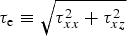 $\tau _{\rm e} \equiv \sqrt {\tau _{xx}^2 + \tau _{xz}^2} $
, is beneath a material dependent yield strength, τ
y, we assume the glacier ice is rigid. In reality glaciers are not rigid beneath a yield strength. However, in our model we assume that the deformation of intact glacier ice is much slower than the deformation of yielded ice—effectively rigid. Above the yield strength τ
y, we assume the ice is disarticulated and flows like a granular material. We model this regime as power-law creep, but with a much smaller effective viscosity then the viscosity of intact ice. Hence, our rheology can be written in the form:
$\tau _{\rm e} \equiv \sqrt {\tau _{xx}^2 + \tau _{xz}^2} $
, is beneath a material dependent yield strength, τ
y, we assume the glacier ice is rigid. In reality glaciers are not rigid beneath a yield strength. However, in our model we assume that the deformation of intact glacier ice is much slower than the deformation of yielded ice—effectively rigid. Above the yield strength τ
y, we assume the ice is disarticulated and flows like a granular material. We model this regime as power-law creep, but with a much smaller effective viscosity then the viscosity of intact ice. Hence, our rheology can be written in the form:
 $$\tau _{ij} = \displaystyle{1 \over {\dot \gamma}} \left( {B_{{\rm gran}}\;{\dot \gamma} ^{1/n} + \tau _{\rm y}} \right)\;\dot \varepsilon _{ij}\quad {\rm for}\;\tau _{\rm e} \ge \tau _{\rm y},$$
and $\dot \varepsilon _{ij} \equiv 0$
otherwise. Here B
gran represents the softness parameter for yielded (granular) ice, the components of the strain rate tensor are
$\dot \varepsilon _{ij} \equiv 0$
otherwise. Here B
gran represents the softness parameter for yielded (granular) ice, the components of the strain rate tensor are $\dot \varepsilon _{ij} = \left( {(\partial u_i/\partial x_j) + (\partial u_j/\partial x_i)} \right)$
, and
$\dot \varepsilon _{ij} = \left( {(\partial u_i/\partial x_j) + (\partial u_j/\partial x_i)} \right)$
, and
 $$\dot \gamma = \sqrt {4\dot \varepsilon _{xx}^2 + \dot \varepsilon _{xz}^2} \equiv 2\dot \varepsilon _{\rm e},$$
defining $\dot \varepsilon _{\rm e}$
as the effective strain rate.
$\dot \varepsilon _{\rm e}$
as the effective strain rate.
We impose two boundary conditions: the upper surface must be traction-free, and for simplicity we require no slip at the bed. The no-slip boundary condition means simply that both velocity components vanish at the bed b(x), i.e.
 $$u = w = 0\;\;\;{\rm wherever}\;z = b(x).$$
The ice/air interface z = h(x,t) is a material surface subject to net snow accumulation, $\dot a$
. Imposing the traction-free condition on this material surface gives the boundary conditions:
$\dot a$
. Imposing the traction-free condition on this material surface gives the boundary conditions:
 $$\displaystyle{{\partial h} \over {\partial t}} + u\displaystyle{{\partial h} \over {\partial x}} = w + \dot a,$$
 $$\left( {1 - {\left( {\displaystyle{{\partial h} \over {\partial x}}} \right)}^2} \right)p + \left( {1 + {\left( {\displaystyle{{\partial h} \over {\partial x}}} \right)}^2} \right)\tau _{xx} = 0,$$
 $$\left( {1 - {\left( {\displaystyle{{\partial h} \over {\partial x}}} \right)}^2} \right)\tau _{xz} - 2\displaystyle{{\partial h} \over {\partial x}}\tau _{xx} = 0.$$
We now nondimensionalize our equations using a characteristic thickness H, a characteristic length scale L, and the aspect ratio ε = H/L. Then
 $$u = V\tilde u\quad\quad w = {\rm \epsilon} V\tilde w\quad\quad t = \displaystyle{L \over V}\tilde t$$
 $$p = {\rho gH\tilde p}\quad\quad {\dot \gamma} = \displaystyle{V \over H}\tilde {\dot \gamma} \quad\quad {\tau _{ij}} = \rho \nu \displaystyle{V \over H}\tilde \tau _{ij}$$
 $$\displaystyle{\partial \over {\partial x}} = \displaystyle{1 \over L}\displaystyle{\partial \over {\partial \tilde x}}\quad\quad \displaystyle{\partial \over {\partial z}} = \displaystyle{1 \over H}\displaystyle{\partial \over {\partial \tilde z}}\quad\quad \displaystyle{\partial \over {\partial t}} = \displaystyle{V \over L}\displaystyle{\partial \over {\partial \tilde t}}$$
where ρ = ρ
ice (assumed constant), V = gH
3/νL is a characteristic flow speed, $\nu = B_{{\rm gran}}(V/H)^{(1/n) - 1}/\rho $
is a characteristic viscosity, and tildes denote dimensionless variables. This nondimensionalization corresponds to a model where the characteristic timescale is determined by the (assumed) much faster timescale associated with rapid flow of yielded ice. On this fast timescale, unyielded ice appears to be quasi-rigid.
$\nu = B_{{\rm gran}}(V/H)^{(1/n) - 1}/\rho $
is a characteristic viscosity, and tildes denote dimensionless variables. This nondimensionalization corresponds to a model where the characteristic timescale is determined by the (assumed) much faster timescale associated with rapid flow of yielded ice. On this fast timescale, unyielded ice appears to be quasi-rigid.
In the final dimensionless equations, we drop the tilde markers for ease of notation. The conservation equations become:
 $$\displaystyle{{\partial u} \over {\partial x}} + \displaystyle{{\partial w} \over {\partial z}} = 0$$
 $${\epsilon {\cal R}}\left( {\displaystyle{{\partial u} \over {\partial t}} + u\displaystyle{{\partial u} \over {\partial x}} + w\displaystyle{{\partial u} \over {\partial z}}} \right) = - \displaystyle{{\partial p} \over {\partial x}} + {\epsilon} \displaystyle{\partial \over {\partial x}}\tau _{xx} + \displaystyle{\partial \over {\partial z}}\tau _{xz}$$
 $${\epsilon} ^3{\rm {\cal R}}\left( {\displaystyle{{\partial w} \over {\partial t}} + u\displaystyle{{\partial w} \over {\partial x}} + w\displaystyle{{\partial w} \over {\partial z}}} \right) = - \displaystyle{{\partial p} \over {\partial z}} + {\epsilon} ^2\displaystyle{\partial \over {\partial x}}\tau _{xz} + {\epsilon} \displaystyle{\partial \over {\partial z}}\tau _{zz} - 1$$
and the rheology
 $$\left( {\matrix{ {\tau _{xx}} & {\tau _{xz}} \cr {\tau _{xz}} & {\tau _{zz}} \cr}} \right) = \displaystyle{1 \over {\dot \gamma}} \left[ {{\dot \gamma} ^{{1 \over n}} + {\rm {\cal B}}} \right]\left( {\matrix{ {2{\epsilon} \displaystyle{{\partial u} \over {\partial x}}} & {\displaystyle{{\partial u} \over {\partial z}} + {\epsilon} ^2\displaystyle{{\partial w} \over {\partial z}}} \cr {\displaystyle{{\partial u} \over {\partial z}} + {\epsilon} ^2\displaystyle{{\partial w} \over {\partial z}}} & {2{\epsilon} \displaystyle{{\partial w} \over {\partial z}}} \cr}} \right)$$
for $\tau _{\rm e} \ge {\rm {\cal B}}$
, with the aspect ratio ε = H/L as above; and
$\tau _{\rm e} \ge {\rm {\cal B}}$
, with the aspect ratio ε = H/L as above; and $\dot \varepsilon _{ij} \equiv 0$
for
$\dot \varepsilon _{ij} \equiv 0$
for $\tau _{\rm e} \lt {\rm {\cal B}}$
. In the above we have introduced the dimensionless Reynolds and Bingham numbers
$\tau _{\rm e} \lt {\rm {\cal B}}$
. In the above we have introduced the dimensionless Reynolds and Bingham numbers
 $${\rm {\cal R}} = \displaystyle{{HV} \over \nu}, \quad {\rm {\cal B}} = \displaystyle{{\tau _yH} \over {\rho \nu V}}.$$
For glaciers and ice sheets, we have ${\rm {\cal R} \ll} 1$
.
${\rm {\cal R} \ll} 1$
.
2.2. Thin film approximation
We take the thin film approximation ${\epsilon \ll} 1$
and drop all terms of order ε or higher to find the simplified equations:
${\epsilon \ll} 1$
and drop all terms of order ε or higher to find the simplified equations:
 $$\displaystyle{{\partial u} \over {\partial x}} + \displaystyle{{\partial w} \over {\partial z}} = 0$$
 $$\displaystyle{{\partial p} \over {\partial x}} = \displaystyle{\partial \over {\partial z}}\tau _{xz}$$
 $$\displaystyle{{\partial p} \over {\partial z}} = - 1$$
 $$\tau _{xz} = \displaystyle{1 \over {\dot \gamma}} \left[ {{\dot \gamma} ^{{1 \over n}} + {\rm {\cal B}}} \right]\displaystyle{{\partial u} \over {\partial z}}.$$
We integrate Eqns (19) and (20) in z, using the boundary conditions p = τ xz = 0 on z = h(x,t), to find
 $$p = h - z\quad\quad \tau _{xz} = - \displaystyle{{\partial h} \over {\partial x}}(h - z),$$
and substitute into the simplified Eqns (18–21) to find the velocity components.
Velocity components described by the rheology (Eqn (16)) are distinct above and below a yield surface,
 $$z = Y(x,t) = \max \left( {h - \displaystyle{{\rm {\cal B}} \over { \vert \partial h/\partial x \vert}}, b(x)} \right)$$
(also Balmforth and others, Reference Balmforth, Craster, Rust and Sassi2006). In the perfect plastic approximation, the yield surface is everywhere coincident with the bed. That is, either an infinitesimal layer of ice or the bed itself is yielding and the rest of the glacier is intact. This approximation produces a nonlinear first-order differential equation for glacier surface elevation:
 $$ \vert h - b \vert \displaystyle{{\partial h} \over {\partial x}} = {\rm {\cal B}}.$$
2.3. A self-consistent terminus position
In steady state, stresses at the glacier terminus from ice and seawater must balance. That is,
 $$\int_{b(x)}^{h(x)} \sigma _{xx} \,{\rm d}z= \int_{b(x)}^{0} - \rho _wgz\, {\rm d}z.$$
If x = 0 defines the calving front, positions x > 0 lie within the glacier and positions x < 0 lie in the water. We assume that across the calving front, where intact ice transitions to yielded, granular ice, there is another yielding surface, such that lateral stress τ
xx
≊ τ
y
for x ≈ 0+. Then $\sigma _{xx} = 2\tau _{\rm y} - \rho _ig(h - z)$
. Integrating and nondimensionalizing, we find an equation relating terminus ice thickness and water depth analogous to that proposed by Bassis and Walker (Reference Bassis and Walker2012):
$\sigma _{xx} = 2\tau _{\rm y} - \rho _ig(h - z)$
. Integrating and nondimensionalizing, we find an equation relating terminus ice thickness and water depth analogous to that proposed by Bassis and Walker (Reference Bassis and Walker2012):
 $$H_{{\rm terminus}} = 2{\rm {\cal B}\epsilon} + \sqrt {\displaystyle{{\rho _wD^2} \over {\rho _i}} + {\left( {2{\rm {\cal B}\epsilon}} \right)}^2} $$
where $H_{{\rm terminus}} \equiv h(x_{{\rm terminus}}) - b(x_{{\rm terminus}})$
is the dimensionless terminus thickness, ρ
w the density of seawater, D dimensionless water depth and other terms as before. For most cases, the stress-balance requirement is stronger than requiring a grounded terminus—that is, termini that would otherwise thin to flotation instead break and retreat under our model—but we also explicitly require that ice breaks if it thins below flotation thickness:
$H_{{\rm terminus}} \equiv h(x_{{\rm terminus}}) - b(x_{{\rm terminus}})$
is the dimensionless terminus thickness, ρ
w the density of seawater, D dimensionless water depth and other terms as before. For most cases, the stress-balance requirement is stronger than requiring a grounded terminus—that is, termini that would otherwise thin to flotation instead break and retreat under our model—but we also explicitly require that ice breaks if it thins below flotation thickness:
 $$H_{{\rm float}} = D\displaystyle{{\rho _i} \over {\rho _w}}.$$
Each point (x, z) lies on at most one glacier surface elevation profile. Thus, the terminus position and thickness $(x_{{\rm terminus}},H_{{\rm terminus}})$
uniquely determine a profile, and we can implement this condition in numerical solution of the model to simulate terminus advance/retreat connected with upstream thickening/thinning. We note that our simple relation does not imply causality in either direction: terminus retreat can trigger thinning upstream or vice versa.
$(x_{{\rm terminus}},H_{{\rm terminus}})$
uniquely determine a profile, and we can implement this condition in numerical solution of the model to simulate terminus advance/retreat connected with upstream thickening/thinning. We note that our simple relation does not imply causality in either direction: terminus retreat can trigger thinning upstream or vice versa.
2.4. Numerical solution
The surface elevation equation can be solved analytically for some very simple bed geometries. For more complicated geometries, straightforward numerical integration over a given bed function produces the glacier profile. We evolve the surface elevation function h(x) along a centerline described by points $(x_1,x_2, \ldots, x_N)$
using a discretized version of Eqn (24),
$(x_1,x_2, \ldots, x_N)$
using a discretized version of Eqn (24),
 $$h(x_{i + 1}) = \displaystyle{{\tau _{\rm y}} \over {\rho _ig(h(x_i) - b(x_i))}}\Delta x + h(x_i),$$
where $\Delta x = {\rm \parallel} x_{i + 1} - x_i{\rm \parallel} $
, the step size. The bed function b(x) may be defined by an analytical function or by providing observed bed values at the sample points.
$\Delta x = {\rm \parallel} x_{i + 1} - x_i{\rm \parallel} $
, the step size. The bed function b(x) may be defined by an analytical function or by providing observed bed values at the sample points.
We define the coordinate system such that the initial terminus position x terminit = 0. The model may be run: (1) starting from the terminus and stepping Δx > 0 upstream, making use of the water balance condition (Eqn (26)) to determine the initial terminus thickness H terminit, or (2) starting from some upstream position x up > 0 and stepping Δx < 0 downstream, using Eqn (26) to find the terminus position of the resulting profile.
Key symbols and their representative values appearing in this work

3. IDEALIZED GEOMETRIES
To test the functionality of the model, we first examine cases for which there is an analytical solution, such as a constant slope b(x) = mx, and then explore some simple idealized geometries such as concave slopes, sinusoids and slopes with Gaussian bumps. The idealized geometries, inspired by Oerlemans (Reference Oerlemans2008), are chosen to be relevant to outlet glaciers. We test the model using a realistic range of yield strengths, 50–300 kPa, to examine the effect of τ y in idealized cases.
The height of ice cliffs at the terminus depends on water depth D and yield strength τ y (see Table 1). For realistic values of D and τ y, the model produces terminus thicknesses comparable with diverse observations (e.g. Bassis and Walker, Reference Bassis and Walker2012). This is illustrated in Figure 1.
Height of ice cliffs at the terminus produced by the model for yield strengths $\tau _{\rm y} = 50{\kern 1pt} \,{\rm kPa}$
(solid), 150 kPa (dashed), and 500 kPa (dotted) and water depths 0 m
$\tau _{\rm y} = 50{\kern 1pt} \,{\rm kPa}$
(solid), 150 kPa (dashed), and 500 kPa (dotted) and water depths 0 m $ \le D \le 500{\kern 1pt} \,{\rm m}$
.
$ \le D \le 500{\kern 1pt} \,{\rm m}$
.

To model terminus retreat associated with thinning, we identify an up-glacier reference point on the centerline where thinning will be simulated. We evolve the model from the terminus upstream to create a reference profile and find the reference ice thickness at the chosen point. Then, we vary the ice thickness at the reference point and evolve the model downstream from the reference point, requiring that the ice break if it thins below what is permitted by Eqns (26) and (27). This allows us to find the terminus position associated with a given amount of thinning.
Our tests show that the plastic model is able to produce realistic glacier profiles and retreat patterns over idealized bed geometries. Figure 2a shows snapshots of retreat using the perfect plastic approximation over a constant seaward-sloping bed. We note the familiar ‘pancake’ profile visible in each successive snapshot. With constant upstream thinning of 5 m a–1, the glacier terminus initially retreats quickly: about 12 km in the first 10 years. The initial rapid retreat pulls the terminus above sea level, however, and subsequent retreat is less dramatic.
Retreat of a perfectly plastic glacier under 5 m a–1 constant upstream thinning. Colored curves show initial profile (black) and profiles (blue scale) after 10, 20, 30 and 40 a of thinning. The idealized bed cases (after Oerlemans, Reference Oerlemans2008) shown are: (a) constant seaward-sloping bed, (b) seaward-sloping bed with overdeepening and submerged sill and (c) concave bed.
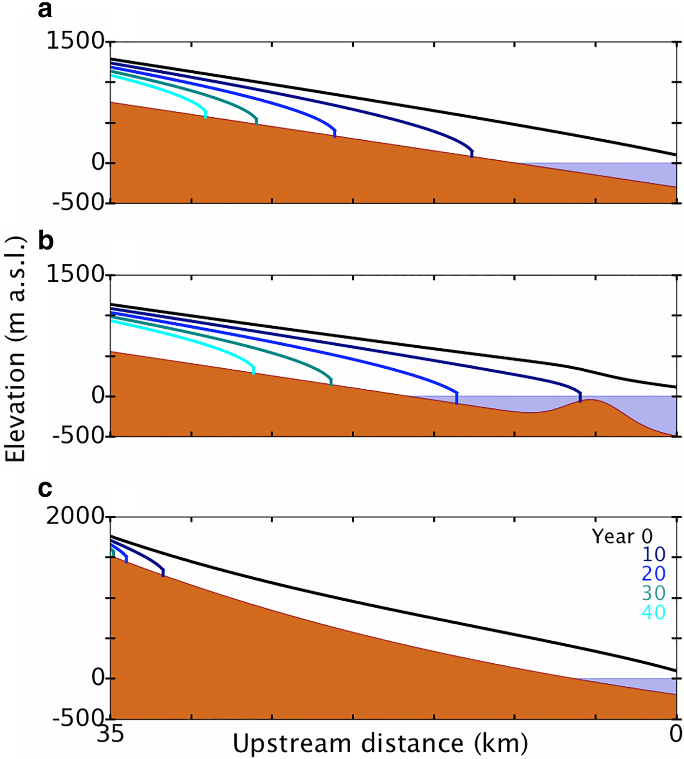
In Figure 2b, we have imposed the same constant upstream thinning rate on a perfectly plastic glacier with an overdeepening and submerged sill in its bed. The initial retreat of this glacier is less rapid; it stabilizes temporarily on the submerged sill before continuing to retreat. Once again, retreat is more pronounced while the terminus is grounded below sea level and becomes more gradual after retreat pulls the terminus above sea level, consistent with observations that only marine- (and lake-) terminating glaciers retreat rapidly.
Figure 2c shows retreat over a concave bed. The concave idealized bed represents the case of bed slope decreasing downstream, as when a glacier descends from high mountains before traversing a coastal plain (or simply a shallower valley) and terminating in the ocean. The initial steady-state profile shows a long glacier with terminus grounded in 200 m of water. Imposing the same constant thinning as in cases (a) and (b), however, shows markedly different results. After just 10 years, the glacier has retreated more than 30 km, finally stabilizing more than 1000 m above sea level (a.s.l.). Subsequent retreat is more gradual, but within 30 years, the glacier has all but disappeared.
4. CASE STUDY: COLUMBIA GLACIER
We next apply our model to the more realistic geometry of the Columbia Glacier, located in south-central Alaska (inset, Fig. 3). After several decades of relative stability in the early 20th century, the Columbia Glacier has been changing rapidly since 1980, retreating more than 20 km (McNabb and others, Reference McNabb2012) and thinning up to 20 m a–1 on a regional scale (O'Neel and others, Reference O'Neel, Pfeffer, Krimmel and Meier2005). The extensive data collected since 1957 make the Columbia Glacier one of the most well-studied tidewater glaciers in the world. A dataset published by McNabb and others (Reference McNabb2012) provides reconstructed bed topography and ice thickness, based on velocity observations of the Columbia Glacier and mass conservation. Surface elevation for 1957 is digitized from the USGS National Elevation Dataset, with 2007 surface elevation based on a panchromatic image from the SPOT (Satellite Pour l'Observation de la Terre) satellite. Calculated ice thickness is provided for both 1957 and 2007, effectively showing the state of the glacier before and during its recent major retreat.
Columbia Glacier main centerline shown in white, with red ticks every 5 km, over a map of bed elevation. Inset in top right corner shows the location of Columbia Glacier (red star) over an outline of the state of Alaska. Northing and easting coordinates refer to Universal Transverse Mercator zone 6V.

The main branch of Columbia begins on high mountains (Fig. 3), nearly 2500 m a.s.l. The bed initially slopes steeply downward (as in ideal case (a)), with an especially steep icefall ~45 km upstream from the pre-retreat terminus. After the icefall, the bed slope becomes more shallow (as in ideal case (c)) and is grounded below sea level for >30 km, with several small sills. A prominent sill ~20 km upstream from the pre-retreat terminus has been a site of stabilization since 2010 for the main branch retreat (as in ideal case (b)). Key features of the Columbia bed topography, illustrated in brown in Figures 4 and 5, can be compared with Figure 2 above. These features, along with the available bed topography and ice thickness data from several years of study, motivate selection of Columbia Glacier as an initial study site. In this case study, we test our model using realistic bed topography from observations of Columbia and comparing the modeled surface elevation profiles with observed glacier profiles. Figure 3 shows the chosen main branch centerline on a map of Columbia Glacier bed topography.
Columbia Glacier main centerline: perfect plastic model profiles ( $\tau _{\rm y} = 150 \,{\rm kPa}$
, solid curves) with 1957 and 2007 observations (dashed curves). Note 5:1 vertical exaggeration in scale.
$\tau _{\rm y} = 150 \,{\rm kPa}$
, solid curves) with 1957 and 2007 observations (dashed curves). Note 5:1 vertical exaggeration in scale.

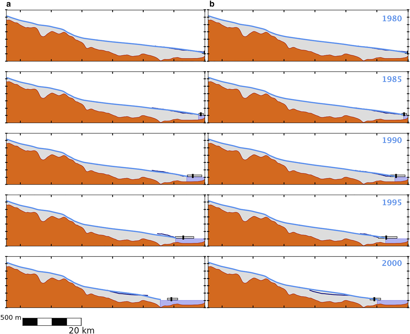
Five-yearly snapshots of Columbia Glacier retreat, with the top frames representing 1980 and the bottom frames representing 2000. Model results appear as light blue filled profiles, USGS flightline elevation profiles as navy blue curves, centroid terminus positions as vertical black markers with grey observational range. Scalebar at bottom left shows scales of 20 km in the horizontal and 500 m in the vertical. Panels: (a) retreat simulated with constant $\tau _{\rm y} = 150{\kern 1pt} \,{\rm kPa}$
; (b) retreat simulated with the effective pressure criterion,
$\tau _{\rm y} = 150{\kern 1pt} \,{\rm kPa}$
; (b) retreat simulated with the effective pressure criterion, $\tau _{\rm y} = 130\,{\rm kPa} + \mu (\rho _igH - \rho _{\rm w}gD)$
.
$\tau _{\rm y} = 130\,{\rm kPa} + \mu (\rho _igH - \rho _{\rm w}gD)$
.
4.1. Steady-state profiles
We manually define a centerline along Columbia's main branch by choosing a set of points on a contour plot of 1957 ice thickness, and we interpolate the bed and ice elevation data to 1-D functions in terms of arc length along the centerline. Using the bed function defined by the data, we model the glacier surface elevation along the centerline according to Eqn (28). We apply the model using a range of different yield strengths τ y. The value is constrained by observations and laboratory experiments; the range 50–200 kPa considered in the idealized case reflects an appropriate range (O'Neel and others, Reference O'Neel, Pfeffer, Krimmel and Meier2005; Cuffey and Paterson, Reference Cuffey and Paterson2010).
In the simplest case, we assume τ y is constant. Because τ y reflects the shear strength at the bed in our approximation, τ y may vary spatially or with time. For example, there may be soft marine sediments with low τ y near the terminus and hard bedrock with high τ y upstream. The effects of subglacial processes such as erosion, sediment deposition, and evolving water drainage suggest temporal variation in τ y as well. We can introduce a physically-motivated modification to the model by allowing τ y to be a function of effective water pressure at the glacier base, implemented as follows:
 $$\tau _{\rm y} = \tau _0 + \mu \left( {\rho _ig(h - b) - \rho _wgD} \right),$$
with μ ≊ 0.01 the bulk coefficient of friction and all other symbols as previously defined. Our choice of μ reflects the lower end of the range derived experimentally by Cohen and others (Reference Cohen2005) and is of the appropriate order of magnitude to fit observed Columbia profiles.
The model produces a realistic central profile that can be compared with observations from 1957 and 2007. The shape of the profile is determined by the yield strength, with values of τ
y between 75 and 220 kPa producing the most realistic profiles. Force balance calculations by O'Neel and others (Reference O'Neel, Pfeffer, Krimmel and Meier2005) suggest a probable range of yield strengths for the Columbia Glacier bed of 50–200 kPa. The perfect plastic profiles computed with $\tau _{\rm y} = 150{\kern 1pt} \,{\rm kPa}$
for the 1957 and 2007 observed terminus positions are shown in Figure 4, with observed 1957 and 2007 profiles presented for comparison.
$\tau _{\rm y} = 150{\kern 1pt} \,{\rm kPa}$
for the 1957 and 2007 observed terminus positions are shown in Figure 4, with observed 1957 and 2007 profiles presented for comparison.
When observations of surface elevation are available for the entire centerline, as for 1957 and 2007, the CV RMS statistic (coefficient of variation of the RMSE) comparing simulated and observed ice thickness is defined and we may use it for analysis. The CV RMS is related to RMSE but normalized by the mean value of the measurement. This normalization reflects the physical intuition that 100 m of error on a 100 m-thick glacier is more problematic than 100 m of error on a 1000 m-thick glacier.
Allowing yield strength to vary with effective basal pressure produces steady-state profiles with CV
RMS
comparable with that of constant yield profiles. The shape of variable-τ
y profiles depends on the choice of τ
0 in Eqn (29); CV
RMS
is minimized using τ
0 ≊ 130 kPa. Note that the coefficient of friction μ in Eqn (29) also affects the shape of the glacier profiles, but for this study we have held μ = 0.01 constant. Visually, the centerline profiles computed for 1957 and 2007 using $\tau _{\rm y} = 130\,{\rm kPa} + \mu (\rho _igH - \rho _wgD)$
are nearly indistinguishable from the constant-τ
y profiles shown in Figure 4.
$\tau _{\rm y} = 130\,{\rm kPa} + \mu (\rho _igH - \rho _wgD)$
are nearly indistinguishable from the constant-τ
y profiles shown in Figure 4.
4.2. Retreat
To simulate retreat, we proceed as described for the idealized cases. We assume that the glacier surface elevation was approximately constant during its decades of stability (until about 1980) and that all observed thinning occurred 1982–2007, during the recent period of rapid retreat (Krimmel, Reference Krimmel2001; O'Neel and others, Reference O'Neel, Pfeffer, Krimmel and Meier2005). Further, we assume a constant thinning rate between 1982 and 2007—this works out to an average 8 m a−1 at the reference point 35 km upstream. Using this thinning rate, we can estimate the amount of thinning corresponding to a particular month or year during Columbia's retreat and generate a snapshot of the centerline profile at that time. We ‘evolve’ the model in time by producing a series of such snapshots. We then evaluate the model by comparing snapshots from a particular year with surface elevation and terminus position data obtained in that year by the USGS (Krimmel, Reference Krimmel2001). Note that while we time-evolve the model by controlling upstream thinning, it could just as well be time-evolved by controlling the terminus retreat rate and solving for upstream thickness. That is, the apparent ‘causality’ in the model could be reversed. We do not presume to comment on the correct direction of causality. Figure 5 shows 5-yearly snapshots of the retreat simulated with $\tau _{\rm y} = 150{\kern 1pt} \,{\rm kPa}$
and
$\tau _{\rm y} = 150{\kern 1pt} \,{\rm kPa}$
and $\tau _{\rm y} = 130\,{\rm kPa} + \mu (\rho _igH - \rho _{\rm w}gD)$
. Animations of the modeled retreat are available in the Supplementary Information.
$\tau _{\rm y} = 130\,{\rm kPa} + \mu (\rho _igH - \rho _{\rm w}gD)$
. Animations of the modeled retreat are available in the Supplementary Information.
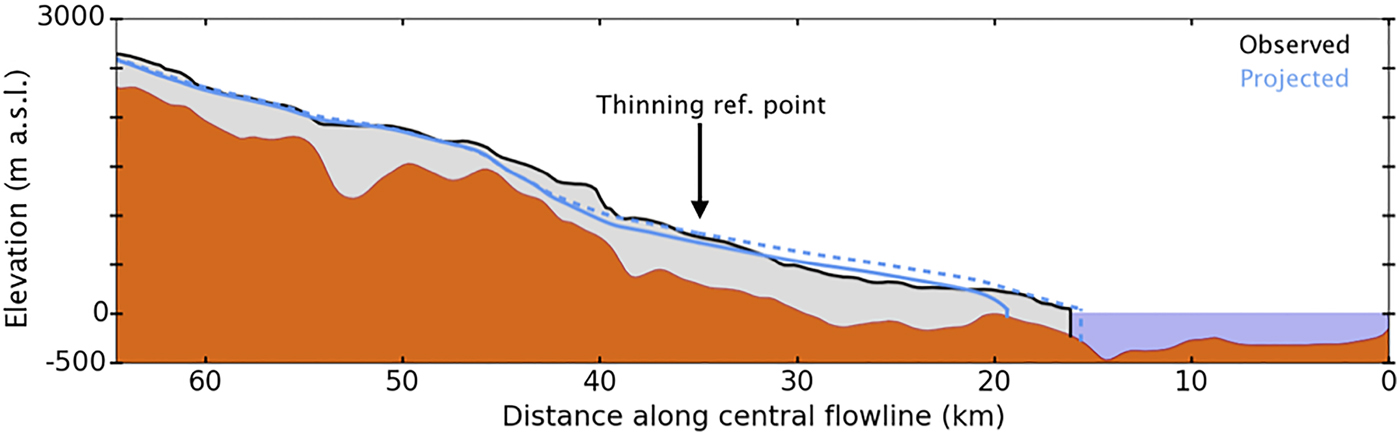
Differences between the yield criteria are more immediately visible in a direct comparison. Figure 6 shows the two profiles produced by prescribing the amount of thinning observed in the period 1957–2007 at the reference point. We notice that the profile produced using the effective pressure yield criterion reaches a terminus position ~0.6 km farther advanced than the 2007 observation, while the profile from the constant yield criterion has a terminus ~3.2 km farther retreated than the 2007 observation. The difference in performance can also be seen in the Supplementary Animations S1 $(\tau _{\rm y} = 150\,{\kern 1pt} {\rm kPa})$
and S2
$(\tau _{\rm y} = 150\,{\kern 1pt} {\rm kPa})$
and S2 $(\tau _{\rm y} = 130\,{\rm kPa} + \mu (\rho _igH - \rho _{\rm w}gD))$
.
$(\tau _{\rm y} = 130\,{\rm kPa} + \mu (\rho _igH - \rho _{\rm w}gD))$
.
Comparison of constant yield and effective-pressure yield criteria in simulating 2007 retreat from prescribing observed amount of thinning (210 m) at reference point (35 km upstream, black arrow). The centerline profile from 2007 observation (McNabb and others, Reference McNabb2012) appears with black outline and grey fill. Profiles projected using $\tau _{\rm y} = 150\,{\kern 1pt} {\rm kPa}$
and
$\tau _{\rm y} = 150\,{\kern 1pt} {\rm kPa}$
and $\tau _{\rm y} = 130\,{\rm kPa} + \mu (\rho _igH - \rho _{\rm w}gD)$
are solid and dashed blue curves, respectively.
$\tau _{\rm y} = 130\,{\rm kPa} + \mu (\rho _igH - \rho _{\rm w}gD)$
are solid and dashed blue curves, respectively.
5. DISCUSSION
Results of our idealized simulations compare well with observations of glacier profiles and terminus thicknesses (e.g. Bassis and Walker, Reference Bassis and Walker2012). We have confirmed that the model is able to reproduce advance and retreat of tidewater glaciers over representative bed topographies, and simulations driven with moderate upstream thinning (5 m a–1) show the corresponding retreat matches observations. Note that the choice of reference point is significant—simulating 5 m a–1 of thinning at a point only 10 km upstream from the terminus will produce results quite different from 5 m a–1 thinning at the reference point 35 km upstream. Rapid thinning near sea level and rapid thinning at higher elevation correspond to different climate scenarios, however, and the model responds as we would expect: thinning simulated closer to the terminus will produce less rapid terminus retreat than the same amount of thinning simulated farther upstream.
The retreat scenarios shown in Figure 2 match physical intuition. In Figure 2a, for example, rapid retreat levels off once the glacier terminus is no longer in contact with the ocean. This phenomenon has been documented several times in the literature (Pfeffer, Reference Pfeffer2007; Pfeffer and others, Reference Pfeffer, Harper and O'Neel2008). In Figure 2b, the glacier's initial retreat is modulated by a submarine sill. As the terminus thins in deep water, it no longer satisfies the water-balance conditions of Eqns (26) and (27) and must retreat. When the terminus retreats onto the submarine sill, however, it is able to stabilize in the shallower water. Figure 2c shows an analogous case, though its results may be less intuitive. As the glacier retreats out of the water, the terminus thickness for force-balance decreases (Eqn (26) with D = 0). Even though it is thinning upstream, the downstream portion of the glacier is too thick to form a stable ice cliff on the concave bed, so it retreats rapidly and does not stabilize until the terminus is very close to the ice ‘divide’. In a small neighborhood of the ice divide, the concave bed may locally approximate a constant downhill slope, so we see subsequent retreat proceed accordingly. There is not much glacier left for thinning and retreat, though, and the profile after 30 years of thinning shows only a small scrap of glacier ice remaining. This is perhaps unsurprising, as the ice divide portion of the glacier of Figure 2c was already thinner than the other idealized cases when constant 5 m a–1 thinning began.
The modeled profiles of Columbia Glacier show good agreement with 1957 and 2007 observed ice thickness along the main centerline, and the model reproduces observed retreat and thinning. The model successfully captures the hinge point behavior of the Columbia Glacier noted by McNabb and others (Reference McNabb2012); in both the observations and the model, the most drastic changes to the centerline profile are seen in the lower reaches, below a ‘hinge point’ ~40 km up from the terminus, with ice thickness upstream remaining relatively constant. The amount of retreat corresponding to a given amount of thinning (or equilibrium line altitude perturbation) depends on the yield strength, but using the range of τ y realistic for Columbia we see realistic results. With a constant yield strength of 150 kPa, thinning of the main branch at a reference point just below the hinge point produces retreat consistent with the 1957 and 2007 observations. We also see that the model disagreement with observation (as measured by the CV RMS ) is higher for 2007 profiles, and that the model tends to overestimate 2007 thickness when using a single constant yield strength—consistent with what would be seen if the shear strength of the bed decreased due to subglacial processes between 1957 and 2007. This agrees with observations that suggest low shear strength at the bed of Columbia Glacier in 2007 (Walter and others, Reference Walter2010).
Beyond static profiles, we have also successfully reproduced the general pattern of Columbia's retreat up to 2007, including an acceleration while the terminus retreated off a sill and over an overdeepening in the bed. Both animations (Supplementary Material) capture this behavior, and snapshots can be seen in Figure 5. The glacier simulated with $\tau _{\rm y} = 150{\kern 1pt} \,{\rm kPa}$
shows more retreat over the period 1982–2007 than does the simulation with
$\tau _{\rm y} = 150{\kern 1pt} \,{\rm kPa}$
shows more retreat over the period 1982–2007 than does the simulation with $\tau _{\rm y} = 130\,{\rm kPa} + \mu (\rho _igH - \rho _{\rm w}gD)$
. For straightforward comparison, Figure 6 superimposes the 2007 profiles when retreat is simulated with a constant yield strength and with the effective basal pressure yield criterion. The absolute difference in terminus position between model and 2007 observation is a rough measure of each model variant's skill at simulating retreat. In Figure 6 we see a difference in terminus position of modeled and observed profiles of +0.595 km for the effective pressure case
$\tau _{\rm y} = 130\,{\rm kPa} + \mu (\rho _igH - \rho _{\rm w}gD)$
. For straightforward comparison, Figure 6 superimposes the 2007 profiles when retreat is simulated with a constant yield strength and with the effective basal pressure yield criterion. The absolute difference in terminus position between model and 2007 observation is a rough measure of each model variant's skill at simulating retreat. In Figure 6 we see a difference in terminus position of modeled and observed profiles of +0.595 km for the effective pressure case $\tau _{\rm y} = 130\,{\rm kPa} + \mu (\rho _igH - \rho _{\rm w}gD)$
and –3.171 km for the constant-yield case
$\tau _{\rm y} = 130\,{\rm kPa} + \mu (\rho _igH - \rho _{\rm w}gD)$
and –3.171 km for the constant-yield case $\tau _{\rm y} = 150{\kern 1pt} \,{\rm kPa}$
. By this metric, allowing yield strength to vary with effective basal pressure produces a simulation closer to observations.
$\tau _{\rm y} = 150{\kern 1pt} \,{\rm kPa}$
. By this metric, allowing yield strength to vary with effective basal pressure produces a simulation closer to observations.
Simulations using the effective pressure yield criterion more closely match several available observations, and agree with several studies suggesting that effective basal pressure is an important factor governing tidewater glacier retreat (Vieli and others, Reference Vieli, Funk and Blatter2000; Pfeffer, Reference Pfeffer2007; Truffer and others, Reference Truffer, Motyka, Hekkers, Howat and King2009). In particular, for the year 2000 – the last year for which USGS terminus-position data is available – the terminus position predicted using $\tau _{\rm y} = 150{\kern 1pt} \,{\rm kPa}$
is not within the range of observed terminus positions, while the position predicted using
$\tau _{\rm y} = 150{\kern 1pt} \,{\rm kPa}$
is not within the range of observed terminus positions, while the position predicted using $\tau _{\rm y} = 130\,{\rm kPa} + \mu (\rho _igH - \rho _{\rm w}gD)$
is within that range. For all other years, both simulations place the glacier terminus inside the range given by USGS data. That is, using the slightly more complicated case
$\tau _{\rm y} = 130\,{\rm kPa} + \mu (\rho _igH - \rho _{\rm w}gD)$
is within that range. For all other years, both simulations place the glacier terminus inside the range given by USGS data. That is, using the slightly more complicated case $\tau _{\rm y} = 130\,{\rm kPa} + \mu (\rho _igH - \rho _{\rm w}gD)$
does improve the model, but using the constant yield strength
$\tau _{\rm y} = 130\,{\rm kPa} + \mu (\rho _igH - \rho _{\rm w}gD)$
does improve the model, but using the constant yield strength $\tau _{\rm y} = 150{\kern 1pt} \,{\rm kPa}$
is an acceptable simplification for the main branch of Columbia Glacier.
$\tau _{\rm y} = 150{\kern 1pt} \,{\rm kPa}$
is an acceptable simplification for the main branch of Columbia Glacier.
Specifying that $\tau _{\rm y} = 150{\kern 1pt} \,{\rm kPa}$
is an acceptable choice for the main branch of Columbia Glacier (i.e. perhaps only there) is not trivial. As discussed in Methods, above, we have reason to suspect that τ
y is not constant in space; in particular, its value may be quite different for geographically distant glaciers. Further, in this work we have assumed
$\tau _{\rm y} = 150{\kern 1pt} \,{\rm kPa}$
is an acceptable choice for the main branch of Columbia Glacier (i.e. perhaps only there) is not trivial. As discussed in Methods, above, we have reason to suspect that τ
y is not constant in space; in particular, its value may be quite different for geographically distant glaciers. Further, in this work we have assumed $\tau _{{\rm y}_{{\rm ice}}} = \tau _{{\rm y}_{{\rm bed}}}$
for simplicity, but a variety of glaciological and geological processes may cause either or both yield strengths to change with time. Laboratory observations and inverse methods from field observations constrain the probable values of
$\tau _{{\rm y}_{{\rm ice}}} = \tau _{{\rm y}_{{\rm bed}}}$
for simplicity, but a variety of glaciological and geological processes may cause either or both yield strengths to change with time. Laboratory observations and inverse methods from field observations constrain the probable values of $\tau _{{\rm y}_{{\rm ice}}}$
; it is more difficult to constrain
$\tau _{{\rm y}_{{\rm ice}}}$
; it is more difficult to constrain $\tau _{{\rm y}_{{\rm bed}}}$
on a particular glacier as it requires some knowledge of (or an educated guess about) the subglacial geology. By comparing the observed terminus cliff height with that predicted by our model's water balance condition (Eqn (26)), it is possible to rule out highly improbable values of τ
y for individual glaciers. For example, Columbia Glacier's 1957 terminus was a 108 m ice cliff in 160 m of water, so Figure 1 suggests that very high yield strengths approaching 500 kPa would be inappropriate.
$\tau _{{\rm y}_{{\rm bed}}}$
on a particular glacier as it requires some knowledge of (or an educated guess about) the subglacial geology. By comparing the observed terminus cliff height with that predicted by our model's water balance condition (Eqn (26)), it is possible to rule out highly improbable values of τ
y for individual glaciers. For example, Columbia Glacier's 1957 terminus was a 108 m ice cliff in 160 m of water, so Figure 1 suggests that very high yield strengths approaching 500 kPa would be inappropriate.
Though the simplicity of the model is a great advantage, there are certain oversimplifications that must be addressed. The 1-D centerline approach with yielding at the bed is not suitable in cases where basal drag is not the dominant control on flow: narrow valley glaciers (controlled by wall drag) and floating ice tongues (controlled by longitudinal stresses), for example. Additionally, the present form of the model is too simple to capture the interaction of different stress regimes, and our focus on steady-state solutions ignores shorter-term variability. We note that our case study of Columbia Glacier concludes in 2007, and that between 2007 and 2012 Columbia Glacier displayed several of these more complicated dynamic features, including the development of a floating ice tongue and short-lived cycles of advance and retreat on the order of 500 m (Walter and others, Reference Walter2010; McNabb and others, Reference McNabb2012). Our model error is higher in 2007, consistent with the onset of conditions less suitable for the perfect plastic approximation. The model may also miss some longer-term variability associated with feedback between terminus retreat and upstream thinning. Finally, the prominent role of the bed topography b(x) in the surface-elevation equation leaves the model susceptible to errors from poorly-known bed topography as well as sparse sampling of the centerline bed data in estimating an appropriate bed geometry. In the case of Columbia Glacier, however, our results show little sensitivity to introduction of random noise, varying smoothing intervals, or displacement of the centerline over the bed.
In our current formulation, the perfect plastic limit corresponds to a steady-state glacier that is in equilibrium with climate forcing. Counter-intuitively, surface mass balance does not directly enter into the computation of glacier profiles. In our model formulation, glacier profiles and terminus position evolve in response to a prescribed upstream thinning rate. Mass balance only enters into calculations of mass flux into the ocean, which we have not attempted here. In keeping with the simplicity of the model, one way to introduce climate sensitivity would be to extrapolate upstream thinning rates based on current trends or quadratic or exponential growth in thinning rates. This would provide sensitivity and some bounds on rates of retreat for individual glaciers. More satisfyingly, climate dependence could also be introduced by coupling with a dynamic ice sheet upstream. For example, a large-scale, climate-responsive ice-sheet model (in which tidewater glaciers are otherwise not resolved) could be used to determine the upstream thickness to input into our model. The two models coupled together will respond to projected changes in climate and resolve individual glacier contributions to SLR with minimal additional computational expense. Alternatively, if changes in terminus position are driving increased thinning rates upstream we could instead prescribe a terminus retreat (or advance) rate and use this to determine glacier profiles. This is more challenging because it would require specification of an additional closure relation that specifies calving rate (or rate of terminus advance) and its relation to local climate forcings, such as submarine melt. In the absence of a well-validated calving law, we suggest the first two options as those most consistent with the simplicity of our modeling approach, but we reassert the caveat that the perfect plastic model is unable to distinguish between changes in terminus position due to upstream thinning and changes in upstream thickness due to terminus advance or retreat.
6. CONCLUSION
We have generalized early work in glacier modeling—namely, Nye's 1951 perfect plastic approximation of glacier ice—to present a new, simplified model of tidewater glacier retreat. Results presented here demonstrate that our simple perfect plastic model produces realistic glacier profiles and basic time evolution with very little input data. Using this model, it is straightforward to gain a first-order understanding of tidewater glaciers for which data are extremely limited. This model and slightly more complicated variations such as a full viscoplastic model can be used to inform policy-relevant sea level projections until such time as the state of available data and computational power allows consistent use of state-of-the-art models for that purpose.
Some of the oversimplifications of this perfect plastic model may be addressed using the slightly more complicated viscoplastic rheology. For example, whereas we have approximated intact glacier ice as rigid over our timescales of interest, viscoplastic flow could account for the viscous creep of intact ice and capture the interaction of different stress regimes in the glacier. However, more complicated models are equally susceptible to errors from poorly-known bed topography and other sparse observations. In the absence of high-resolution data for all the world's glaciers, highly simplified models such as our perfect plastic approximation remain an important tool for constraining 21st century sea-level rise. Using only three inputs—bed topography along a centerline, basal shear strength and change in upstream thickness—the perfect plastic model presented here can produce realistic glacier profiles as well as simulate advance and retreat, offering a first-order understanding of glacial contributions to global mean sea level with negligible computational expense.
SUPPLEMENTARY MATERIAL
The supplementary material for this article can be found at http://dx.doi.org/10.1017/jog.2016.108.
ACKNOWLEDGEMENTS
This work was supported by National Science Foundation grant ANT 114085 and the National Oceanic and Atmospheric Administration, Climate Process Team: Iceberg Calving grant NA13OAR4310096. We thank the editors and reviewers S. O'Neel, M. Truffer and D. Benn, all of whom provided thoughtful guidance.


 Open access

