





1. Introduction
Long-period radio transients (LPTs) are a recently discovered class of radio sources characterised by coherent pulsed emission with pulse durations of seconds to minutes, repeating periodically on timescales of tens of minutes to several hours (e.g. see Hurley-Walker et al. Reference Hurley-Walker2022; Hurley-Walker et al. Reference Hurley-Walker2023; Caleb et al. Reference Caleb2024; Dobie et al. Reference Dobie2024; Li et al. Reference Li2024; Wang et al. Reference Wang2025; Anumarlapudi et al. Reference Anumarlapudi2025; Bloot et al. Reference Bloot2025; de Ruiter et al. Reference de Ruiter2025; Dong et al. Reference Dong2025; Lee et al. Reference Lee2025; McSweeney et al. Reference McSweeney2025). These timescales of periodicity are orders of magnitude longer than the millisecond to second timescales of typical pulsars, placing LPTs within or below the ‘death-valley’ of the period-period derivative diagram (Rea et al. Reference Rea2024). In this regime, spin-down powered decay of the magnetic field cannot support the pair-production required to power pulsar emission. Hence LPTs can not be explained by conventional pulsar emission models, raising fundamental questions about how coherent radio emission can be sustained on such timescales.
The small number of LPTs that have been identified to date ( $\sim$
14 at the time of publication, depending on exactly how the class is defined; Rea et al. Reference Rea, Hurley-Walker and Caleb2026) show a rich diversity of radio properties. Some have been routinely active over decades (e.g. Hurley-Walker et al. Reference Hurley-Walker2023) while others appear intermittent and only remain detectable for short windows before switching off (e.g. Hurley-Walker et al. Reference Hurley-Walker2022; Caleb et al. Reference Caleb2024; Dobie et al. Reference Dobie2024; McSweeney et al. Reference McSweeney2025). The emission often shows high degrees of circular and linear polarisation; yet while some sources show evolution in the polarisation position angle (PA) reminiscent of pulsars (Dobie et al. Reference Dobie2024), others display flat or slowly varying PA profiles (Caleb et al. Reference Caleb2024). In some objects the pulse morphology and polarisation remain stable over an active window (Lee et al. Reference Lee2025), while in others these properties change from pulse to pulse, showing a variety of behaviours such as emission mode changes (e.g. Caleb et al. Reference Caleb2024), narrowband structure (e.g. Anumarlapudi et al. Reference Anumarlapudi2025), timing glitches (e.g. Dong et al. Reference Dong2025), frequency- dependent polarisation conversion, and orthogonal mode jumps (e.g. Men et al. Reference Men, McSweeney, Hurley-Walker, Barr and Stappers2025).
$\sim$
14 at the time of publication, depending on exactly how the class is defined; Rea et al. Reference Rea, Hurley-Walker and Caleb2026) show a rich diversity of radio properties. Some have been routinely active over decades (e.g. Hurley-Walker et al. Reference Hurley-Walker2023) while others appear intermittent and only remain detectable for short windows before switching off (e.g. Hurley-Walker et al. Reference Hurley-Walker2022; Caleb et al. Reference Caleb2024; Dobie et al. Reference Dobie2024; McSweeney et al. Reference McSweeney2025). The emission often shows high degrees of circular and linear polarisation; yet while some sources show evolution in the polarisation position angle (PA) reminiscent of pulsars (Dobie et al. Reference Dobie2024), others display flat or slowly varying PA profiles (Caleb et al. Reference Caleb2024). In some objects the pulse morphology and polarisation remain stable over an active window (Lee et al. Reference Lee2025), while in others these properties change from pulse to pulse, showing a variety of behaviours such as emission mode changes (e.g. Caleb et al. Reference Caleb2024), narrowband structure (e.g. Anumarlapudi et al. Reference Anumarlapudi2025), timing glitches (e.g. Dong et al. Reference Dong2025), frequency- dependent polarisation conversion, and orthogonal mode jumps (e.g. Men et al. Reference Men, McSweeney, Hurley-Walker, Barr and Stappers2025).
Multi-wavelength detections are beginning to provide insight into the astrophysical classification of LPTs, and as a result at least two subclasses are emerging. Some LPTs have infrared, optical, or ultraviolet counterparts suggestive of a white dwarf (WD) main-sequence binary system (e.g. de Ruiter et al. Reference de Ruiter2025; Hurley-Walker et al. Reference Hurley-Walker2024; Rodriguez Reference Rodriguez2025; Anumarlapudi et al. Reference Anumarlapudi2025; Bloot et al. Reference Bloot2025). Others show behaviour more consistent with a neutron star progenitor: such as ASKAP J1832 $-$
0911 which produces periodically pulsed X-ray emission (Wang et al. Reference Wang2025). However, the diverse radio phenomenology observed so far does not align neatly with these associations, and more research is required to understand and explain the phenomena.
$-$
0911 which produces periodically pulsed X-ray emission (Wang et al. Reference Wang2025). However, the diverse radio phenomenology observed so far does not align neatly with these associations, and more research is required to understand and explain the phenomena.
The discovery of LPTs has been enabled by widefield facilities, namely the Australian SKA Pathfinder (ASKAP; Johnston et al. Reference Johnston2008; Hotan et al. Reference Hotan2021), the Murchison Widefield Array (MWA; Bowman et al. Reference Bowman2013), the LOw-Frequency ARray (LOFAR; van Haarlem et al. Reference van Haarlem2013), and the Canadian Hydrogen Intensity Mapping Experiment (CHIME; CHIME/FRB Collaboration et al. 2018). The large instantaneous fields of view of these instruments allows widefield radio surveys to prioritise long dwell times or repeat sampling of the sky with high cadence, probing regions of transient parameter space that have been previously inaccessible. Discoveries have also been aided by the development of novel search techniques such as fast-imaging (e.g. Caleb et al. Reference Caleb2024) and circular polarisation searches (e.g. Anumarlapudi et al. Reference Anumarlapudi2025; Lee et al. Reference Lee2025), allowing these new regions of parameter space to be explored.
In this paper we report the discovery of a new long-period transient, ASKAP J142431.2–612611 (hereafter ASKAP J1424), with a 36 min period, identified via a circular polarisation search. The source exhibited stable pulsed emission for eight days before becoming undetectable, limiting the available data but highlighting its intermittent nature. We present these observations to enable and encourage future monitoring and follow-up of this object. In Section 2, we describe the observations and data analysis, and in Section 3 we discuss the radio properties of the source in the context of the growing population of LPTs.
2. Observations and data analysis
2.1. Detection and radio follow-up
We discovered ASKAP J1424 in a circular polarisation search of a 10 h ASKAP observation, conducted on 2025-01-09 (scheduling block SB70271) as part of the Evolutionary Map of the Universe (EMU; Norris et al. Reference Norris2011, Reference Norris2021) survey. We identified ASKAP J1424 in the full-integration images with a flux density of $1.50\pm 0.01\, \mathrm{mJy\,beam}^{-1}$
in Stokes I (total intensity) and
$1.50\pm 0.01\, \mathrm{mJy\,beam}^{-1}$
in Stokes I (total intensity) and $-0.12\pm 0.01\,\mathrm{mJy\,beam}^{-1}$
in Stokes V,Footnote
a
giving a fractional circular polarisation of 8%.
$-0.12\pm 0.01\,\mathrm{mJy\,beam}^{-1}$
in Stokes V,Footnote
a
giving a fractional circular polarisation of 8%.
Following the ASKAP discovery, we conducted a multi-facility radio follow-up campaign with the Australia Telescope Compact Array (ATCA; Wilson et al. Reference Wilson2011), MeerKAT (Jonas Reference Jonas2009), the Parkes 64 m radio telescope (Murriyang), and the Murchison Widefield Array (MWA; Tingay et al. Reference Tingay2013; Wayth et al. Reference Wayth2018). We detected ASKAP J1424 in both ATCA follow-up observations at 2100 MHz, but made no detections with any other facility. The details of all radio follow-up observations are described in Appendix A and summarised in Table 1. We also searched archival radio and multi-wavelength observations, including 60 observations as part of the Rapid ASKAP Continuum Survey (RACS; McConnell et al. Reference McConnell2020; Duchesne et al. Reference Duchesne2023) and Variables And Slow Transients (VAST; Murphy et al. Reference Murphy2021) surveys with ASKAP, but made no detections. Details and limits are provided in Appendix B.
Summary of radio observations of ASKAP J1424 with ASKAP, ATCA, MWA, MeerKAT, and Murriyang. Columns are the observation start time, telescope, project code/SBID, frequency range $\nu_{\mathrm{obs}}$
, and duration
$\nu_{\mathrm{obs}}$
, and duration $t_{\mathrm{obs}}$
.
$t_{\mathrm{obs}}$
.
 $K_s$
-band Gemini observation with Stokes I radio contours from ATCA C3363 observation overlaid. The green ellipse indicates the 5
$K_s$
-band Gemini observation with Stokes I radio contours from ATCA C3363 observation overlaid. The green ellipse indicates the 5 $\sigma$
astrometric uncertainty of
$\sigma$
astrometric uncertainty of $0^{\prime\prime} 9-1^{\prime\prime}9$
. The positions of catalogued VVV sources are indicated with red markers.
$0^{\prime\prime} 9-1^{\prime\prime}9$
. The positions of catalogued VVV sources are indicated with red markers.

2.2 Infrared photometric follow-up
We acquired near infrared observations in the J and $K_S$
bands with the FLAMINGOS-2 instrument on Gemini South on 2025-01-21. We performed standard data reduction using the DRAGONS pipeline (Labrie et al. Reference Labrie2023), and astrometric calibration by extracting source positions with photutils and registering against the proper-motion corrected positions of stars in Gaia DR3 (Gaia Collaboration et al. 2023). Photometric calibration was obtained by matching isolated and unsaturated field stars to the Variables in the Via Lactea survey (VVV; Minniti et al. Reference Minniti2010), yielding zero-point uncertainties of 0.1 and 0.15 mag in the J and
$K_S$
bands with the FLAMINGOS-2 instrument on Gemini South on 2025-01-21. We performed standard data reduction using the DRAGONS pipeline (Labrie et al. Reference Labrie2023), and astrometric calibration by extracting source positions with photutils and registering against the proper-motion corrected positions of stars in Gaia DR3 (Gaia Collaboration et al. 2023). Photometric calibration was obtained by matching isolated and unsaturated field stars to the Variables in the Via Lactea survey (VVV; Minniti et al. Reference Minniti2010), yielding zero-point uncertainties of 0.1 and 0.15 mag in the J and $K_S$
bands, respectively. In Figure 1, we show a cutout image of the
$K_S$
bands, respectively. In Figure 1, we show a cutout image of the $K_S$
-band data with contours of our ATCA C3363 observation overlaid. We did not detect a source within the
$K_S$
-band data with contours of our ATCA C3363 observation overlaid. We did not detect a source within the $5\sigma$
astrometric uncertainty of
$5\sigma$
astrometric uncertainty of $0^{\prime\prime} 9-1^{\prime\prime} 9$
in either band, with 3
$0^{\prime\prime} 9-1^{\prime\prime} 9$
in either band, with 3 $\sigma$
limiting magnitudesFootnote
b
of
$\sigma$
limiting magnitudesFootnote
b
of $J \gt 22.5$
and
$J \gt 22.5$
and $K_S \gt 19.5$
.
$K_S \gt 19.5$
.
2.3 Time-domain analysis
We processed all calibrated radio observations by forming a model of background sources of emission with WSclean (Offringa et al. Reference Offringa2014), and extracting model-subtracted dynamic spectra in all Stokes parameters using DStools Footnote c (Pritchard Reference Pritchard2025). We then frequency-averaged the dynamic spectra to form visibility lightcurves.
We fit Gaussian profiles to each detected pulse and used the barycentred times of arrival to determine an ephemeris of the form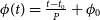 $\phi(t) = \frac{t - t_0}{P} + \phi_0$
, with a best fit period
$\phi(t) = \frac{t - t_0}{P} + \phi_0$
, with a best fit period $P = 2147.27 \pm 0.01\,\mathrm{s}$
. The reference time
$P = 2147.27 \pm 0.01\,\mathrm{s}$
. The reference time $t_0 = {}$
2025-01-09 20:32:11.701 corresponds to the barycentric time of arrival of the first fully sampled pulse in SB70271, with a reference pulse phase of
$t_0 = {}$
2025-01-09 20:32:11.701 corresponds to the barycentric time of arrival of the first fully sampled pulse in SB70271, with a reference pulse phase of $\phi_0 = 0.5$
. The sequence of 17 consecutive pulses detected in this observation uniquely constrains the period and rules out alias periods. Owing to the small time range spanned by the 2025 detections, we are unable to meaningfully constrain the source’s spin-up or spin-down and place an upper limit of order
$\phi_0 = 0.5$
. The sequence of 17 consecutive pulses detected in this observation uniquely constrains the period and rules out alias periods. Owing to the small time range spanned by the 2025 detections, we are unable to meaningfully constrain the source’s spin-up or spin-down and place an upper limit of order $10^{-8}\,\mathrm{s\,s}^{-1}$
on the period derivative.
$10^{-8}\,\mathrm{s\,s}^{-1}$
on the period derivative.
We used this ephemeris to phase-fold all radio observations. Several archival observations obtained between 2021-02-01 and 2024-10-03 sample a significant fraction of the estimated pulse window yet show no emission, suggesting that ASKAP J1424 was not active for multiple years prior to the 2025-01-09 detection. However, it is possible that ASKAP J1424 has short windows of activity as observed in several other LPTs (e.g. Hurley-Walker et al. Reference Hurley-Walker2022; Caleb et al. Reference Caleb2024; Dobie et al. Reference Dobie2024; McSweeney et al. Reference McSweeney2025), and that such intervals were not sampled by the available archival data. The phase-folded lightcurves for all $\sim\mathrm{GHz}$
observations are presented in Appendix A.
$\sim\mathrm{GHz}$
observations are presented in Appendix A.
Phase-folded dynamic spectra of the 17 pulses detected in SB70271 show frequency-dependent phase shifts across the folded pulse profile. Interpreting these shifts as purely dispersive implies a dispersion measure of $\mathrm{DM} = 1\,400 \pm 100\,\mathrm{pc\,cm}^{-3}$
. However, intrinsic frequency-dependent pulse morphology can produce similar phase offsets. When we allow the pulse profile to vary with frequency while simultaneously fitting for dispersion, the inferred DM decreases to
$\mathrm{DM} = 1\,400 \pm 100\,\mathrm{pc\,cm}^{-3}$
. However, intrinsic frequency-dependent pulse morphology can produce similar phase offsets. When we allow the pulse profile to vary with frequency while simultaneously fitting for dispersion, the inferred DM decreases to ${200 \pm 40}\,\mathrm{pc\, cm}^{-3}$
. As the phase shifts in these data are small compared to the pulse width, dispersion and profile evolution cannot be distinguished. We therefore treat
${200 \pm 40}\,\mathrm{pc\, cm}^{-3}$
. As the phase shifts in these data are small compared to the pulse width, dispersion and profile evolution cannot be distinguished. We therefore treat $1\,400\,\mathrm{pc\, cm}^{-3}$
as a conservative upper limit on the DM under the assumption that the observed phase shifts are entirely dispersive. Details of the dispersion modelling are provided in Appendix C.
$1\,400\,\mathrm{pc\, cm}^{-3}$
as a conservative upper limit on the DM under the assumption that the observed phase shifts are entirely dispersive. Details of the dispersion modelling are provided in Appendix C.
We measured the spectral index $\alpha_\nu$
of ASKAP J1424 in these observations by fitting a power law
$\alpha_\nu$
of ASKAP J1424 in these observations by fitting a power law $S(\nu) \propto \nu^{\alpha_\nu}$
to the peak sample of the phase-folded lightcurves. All detections are well-described by a power law, though
$S(\nu) \propto \nu^{\alpha_\nu}$
to the peak sample of the phase-folded lightcurves. All detections are well-described by a power law, though $\alpha_\nu$
changes from
$\alpha_\nu$
changes from $-1.6$
in the 800–1 088 MHz ASKAP band on 2025-01-09 to
$-1.6$
in the 800–1 088 MHz ASKAP band on 2025-01-09 to $-1.2$
in the 1 100–3 100 MHz ATCA band on 2025-01-15. These observations also show a significant decrease in band-averaged flux density from
$-1.2$
in the 1 100–3 100 MHz ATCA band on 2025-01-15. These observations also show a significant decrease in band-averaged flux density from $\sim$
65 to 12 mJy, which cannot be explained solely by spectral shape. As our MWA observations were acquired quasi-contemporaneously with the ATCA observations, non-detection at 200 MHz suggests a limit on the 200–1 100 MHz spectral index
$\sim$
65 to 12 mJy, which cannot be explained solely by spectral shape. As our MWA observations were acquired quasi-contemporaneously with the ATCA observations, non-detection at 200 MHz suggests a limit on the 200–1 100 MHz spectral index $\alpha_\nu\gt -1$
. It is therefore likely that ASKAP J1424 has a spectral turnover between 200–800 MHz, similar to ASKAP J1832
$\alpha_\nu\gt -1$
. It is therefore likely that ASKAP J1424 has a spectral turnover between 200–800 MHz, similar to ASKAP J1832 $-09$
(Wang et al. Reference Wang2025) and ASKAP J1839
$-09$
(Wang et al. Reference Wang2025) and ASKAP J1839 $-07$
(Lee et al. Reference Lee2025).
$-07$
(Lee et al. Reference Lee2025).
2.4 Polarisation properties
We measured the Faraday rotation measure (RM) of all detected pulses using RM synthesis (Brentjens & de Bruyn Reference Brentjens and de Bruyn2005) with the RM-lite
Footnote
d
implementation of RM-tools (Purcell et al. Reference Purcell, Van Eck, West, Sun and Gaensler2020). All pulses show a simple Faraday dispersion function with a single unresolved peak at an RM of $-222\,\mathrm{rad\,m}^{-2}$
and no evidence for RM variations with pulse phase. In Figure 2 we show the phase-folded, RM-corrected pulse profile of 17 pulses from the ASKAP SB70271 observation. The fractional polarisation is consistent with 100% across the full pulse profile, transitioning from an elliptical state during the first half of the pulse to fully linearly polarised.
$-222\,\mathrm{rad\,m}^{-2}$
and no evidence for RM variations with pulse phase. In Figure 2 we show the phase-folded, RM-corrected pulse profile of 17 pulses from the ASKAP SB70271 observation. The fractional polarisation is consistent with 100% across the full pulse profile, transitioning from an elliptical state during the first half of the pulse to fully linearly polarised.
Folded pulse profile of 17 pulses detected in ASKAP observation SB70271. Lightcurves are formed from frequency-averaged dynamic spectra binned to $2\,000$
pulse phase bins, folded at a period of 2 147.27 s. From bottom to top, panels show full polarisation folded pulse profiles, polarisation position angle, and fractional polarisation. Points in the top two panels are masked below a signal-to-noise ratio (SNR) of
$2\,000$
pulse phase bins, folded at a period of 2 147.27 s. From bottom to top, panels show full polarisation folded pulse profiles, polarisation position angle, and fractional polarisation. Points in the top two panels are masked below a signal-to-noise ratio (SNR) of $S_I/\sigma_{S_I} \lt 5$
.
$S_I/\sigma_{S_I} \lt 5$
.

The PA begins at 70 deg and flattens out at 30 deg as the circular polarisation fraction decreases. The evolution in PA is reminiscent of the S-shaped swing in pulsar PA profiles and commonly explained by the rotating vector model (RVM; Radhakrishnan & Cooke Reference Radhakrishnan and Cooke1969), in which the PA corresponds to the projection of the local magnetic field orientation at the emission site onto the plane of the sky. We used the Markov chain Monte Carlo sampler emcee (Foreman-Mackey et al. Reference Foreman-Mackey, Hogg, Lang and Goodman2013) to fit an RVM profile to the phase-folded ASKAP SB70271 lightcurve with a best fit of $\alpha = 170 \pm 4\,\deg$
,
$\alpha = 170 \pm 4\,\deg$
, $\beta = -0.3 \pm 0.1\,\deg$
,
$\beta = -0.3 \pm 0.1\,\deg$
, $\phi_0 = -8.37 \pm 0.04\,\deg$
, and
$\phi_0 = -8.37 \pm 0.04\,\deg$
, and $\psi_0 = -72.6 \pm 0.3\,\deg$
. Here
$\psi_0 = -72.6 \pm 0.3\,\deg$
. Here $\psi(\phi)$
is the PA as a function of pulse phase
$\psi(\phi)$
is the PA as a function of pulse phase $\phi$
,
$\phi$
, $\alpha$
is the angle between rotation and magnetic axes,
$\alpha$
is the angle between rotation and magnetic axes, $\beta$
is the angle between the magnetic axis and line of sight, and
$\beta$
is the angle between the magnetic axis and line of sight, and $\psi_0$
and
$\psi_0$
and $\phi_0$
are the PA and phase around which the PA swing is centred.
$\phi_0$
are the PA and phase around which the PA swing is centred.
While the RVM provides a good empirical description of the observed PA evolution, it is not clear that the emission mechanism powering ASKAP J1424 produces radiation polarised in the sense of the local magnetic field, as is typically assumed for pulsar emission, nor that the fitted RVM parameters map directly onto a rotational geometry. The fitted offset $\phi_0$
between steepest PA gradient and the total intensity peak is also atypical of most pulsars, for which
$\phi_0$
between steepest PA gradient and the total intensity peak is also atypical of most pulsars, for which $\phi_0$
is generally positive and attributed to aberration and retardation effects associated with finite emission heights (Blaskiewicz et al. Reference Blaskiewicz, Cordes and Wasserman1991).
$\phi_0$
is generally positive and attributed to aberration and retardation effects associated with finite emission heights (Blaskiewicz et al. Reference Blaskiewicz, Cordes and Wasserman1991).
The RVM also only accounts for the linearly polarised component of the emission and does not describe the presence or evolution of circular polarisation. To characterise the full polarisation behaviour we therefore analysed the evolution of the normalised Stokes parameters $(Q/P, U/P, V/P)$
on the Poincaré sphere, where
$(Q/P, U/P, V/P)$
on the Poincaré sphere, where $P = \sqrt{Q^2 + U^2 + V^2}$
. Full details of the Poincaré sphere analysis are provided in Appendix D.
$P = \sqrt{Q^2 + U^2 + V^2}$
. Full details of the Poincaré sphere analysis are provided in Appendix D.
In Figure 3 we show the polarisation state of the folded ASKAP SB70271 pulse profile in a Gnomonic projection of the Poincaré sphere, in which great circles are mapped to straight lines. The data are well fit by a great circle with inclination angle of $\delta = 31.5 \pm 0.6\,\deg$
and intersecting the equator of the sphere at a longitude of
$\delta = 31.5 \pm 0.6\,\deg$
and intersecting the equator of the sphere at a longitude of $2\psi_{\mathrm{eq}} = 64.0 \pm 0.4\,\deg$
, corresponding to a PA of
$2\psi_{\mathrm{eq}} = 64.0 \pm 0.4\,\deg$
, corresponding to a PA of $\psi_{\mathrm{eq}} = 32.0 \pm 0.2\,\deg$
. The great circle trajectory shows only marginal evidence for weak frequency dependence, with inclination angle varying with wavelength as
$\psi_{\mathrm{eq}} = 32.0 \pm 0.2\,\deg$
. The great circle trajectory shows only marginal evidence for weak frequency dependence, with inclination angle varying with wavelength as $\delta \propto \lambda^p$
with
$\delta \propto \lambda^p$
with $p = 0.5 \pm 0.2$
when keeping
$p = 0.5 \pm 0.2$
when keeping $2\psi_{\mathrm{eq}}$
fixed to
$2\psi_{\mathrm{eq}}$
fixed to $32.0\,\deg$
and
$32.0\,\deg$
and $p = 0.21 \pm 0.06$
when allowing it to vary freely. A full description of this model is provided in Appendix D.2.
$p = 0.21 \pm 0.06$
when allowing it to vary freely. A full description of this model is provided in Appendix D.2.
Time evolution of polarisation state in the ASKAP SB70271 folded pulse profile. Points show a Gnomonic projection of the Poincaré sphere normalised by total polarisation $P = \sqrt{Q^2 + U^2 + V^2}$
. The red line shows the best linear fit to the projected data, corresponding to a great circle of inclination
$P = \sqrt{Q^2 + U^2 + V^2}$
. The red line shows the best linear fit to the projected data, corresponding to a great circle of inclination $31.5 \pm 0.6\,\deg$
crossing the equator at
$31.5 \pm 0.6\,\deg$
crossing the equator at $64.0 \pm 0.4\,\deg$
longitude.
$64.0 \pm 0.4\,\deg$
longitude.

3. Discussion and conclusions
We have presented the discovery of a long-period transient, ASKAP J1424, with a 36 min period that exhibits an extremely stable pulse profile over an 8 d activity window, as observed with ASKAP and ATCA across 800–3 100 MHz. The emission is consistent with being 100% polarised across the full pulse profile and evolves along a great circle trajectory on the Poincaré sphere as a function of pulse phase transitioning from an elliptical to fully linearly polarised state.
Evolution of the polarisation state along a great circle may be explained by a fully linearly polarised intrinsic polarisation state which then passes through a linear birefringent medium (LBM) in which the natural modes are linearly polarised (Lyutikov Reference Lyutikov2022; Bera et al. Reference Bera2025). In the Poincaré sphere picture, such a medium applies a fixed rotation to the intrinsic polarisation state about an axis aligned with the LBM natural modes, transforming an intrinsic equatorial great circle trajectory into an inclined great circle. Evolution of the pulse phase-resolved polarisation state along a great circle has been previously observed from the LPT ASKAP J1755-2527 (Dobie et al. Reference Dobie2024), though with lower fractional polarisation and possibly being driven by partially coherent mixing of orthogonal modes (Oswald et al. Reference Oswald, Karastergiou and Johnston2023). Similar behaviour has also been observed in fast radio bursts (Bera et al. Reference Bera2025).
We have not identified an optical or infrared counterpart to ASKAP J1424 in either archival data or targeted follow-up observations. As is the case for the majority of LPTs, ASKAP J1424 is located at low Galactic latitude ( $b \sim -0.5^{\circ}$
) where significant extinction is expected, limiting the constraining power of our optical and infrared limits on the nature of the progenitor. Horváth et al. (Reference Horváth2026) demonstrate that GPM J1839
$b \sim -0.5^{\circ}$
) where significant extinction is expected, limiting the constraining power of our optical and infrared limits on the nature of the progenitor. Horváth et al. (Reference Horváth2026) demonstrate that GPM J1839 $-$
10 is likely a WD binary system, with pulse activity driven by magnetic interaction when the WD magnetic axis intersects the companion’s magnetised wind, and recurring at the beat between WD rotation and orbital periods. Considering similar modulation of the activity of ASKAP J1424, we constrain the activity window of this system to be between 8–141 d based on the ASKAP and ATCA detections and nearest-in-time non-detections. Under the Horváth et al. (Reference Horváth2026) model this would imply a beat period of at least several weeks, possibly months. The lack of detections across two years of the VAST Galactic survey may be difficult to reconcile with quasi-periodic activity windows on timescales of weeks. However this is not a strong constraint, as each VAST observation only samples a third of the period and the observing cadence is longer than the nominal activity window.
$-$
10 is likely a WD binary system, with pulse activity driven by magnetic interaction when the WD magnetic axis intersects the companion’s magnetised wind, and recurring at the beat between WD rotation and orbital periods. Considering similar modulation of the activity of ASKAP J1424, we constrain the activity window of this system to be between 8–141 d based on the ASKAP and ATCA detections and nearest-in-time non-detections. Under the Horváth et al. (Reference Horváth2026) model this would imply a beat period of at least several weeks, possibly months. The lack of detections across two years of the VAST Galactic survey may be difficult to reconcile with quasi-periodic activity windows on timescales of weeks. However this is not a strong constraint, as each VAST observation only samples a third of the period and the observing cadence is longer than the nominal activity window.
Further monitoring (e.g. as part of the planned second phase of the VAST Galactic survey) will allow us to determine whether the observed emission follows an intermittent activity pattern, or was powered by a one-off or stochastic event such as accretion of plasma from a companion. Continued characterisation of the polarisation dynamics of ASKAP J1424 in these observations will also provide insight into the viability of an LBM model in explaining the great circle trajectory of the polarisation state, providing important insights into further understanding the emission mechanism and constraining the plasma properties of the near-source medium.
The second phase of the VAST Galactic survey will begin in early 2026 with a revised observing strategy consisting of several high-cadence observing blocks per year. The VAST Galactic fields will be looped over $\sim$
10 times in the space of a few days, supplementing the fortnightly cadence executed in the first phase of the survey. This strategy will provide stronger constraints on orbital modulation in tight binary orbits and will allow characterisation of pulse evolution over timescales of days, such as the fading observed in ASKAP J1424 and mode switching observed in ASKAP J1935 (Caleb et al. Reference Caleb2024).
$\sim$
10 times in the space of a few days, supplementing the fortnightly cadence executed in the first phase of the survey. This strategy will provide stronger constraints on orbital modulation in tight binary orbits and will allow characterisation of pulse evolution over timescales of days, such as the fading observed in ASKAP J1424 and mode switching observed in ASKAP J1935 (Caleb et al. Reference Caleb2024).
Acknowledgements
Parts of this research were supported by the Australian Research Council Centre of Excellence for Gravitational Wave Discovery (OzGrav), project number CE230100016. DK was supported by NSF grant AST-2511757.
This scientific work uses data obtained from Inyarrimanha Ilgari Bundara, the CSIRO Murchison Radio-astronomy Observatory. We acknowledge the Wajarri Yamaji People as the Traditional Owners and native title holders of the Observatory site. CSIRO’s ASKAP radio telescope is part of the ATNF Australia Telescope National Facility. Operation of ASKAP is funded by the Australian Government with support from the National Collaborative Research Infrastructure Strategy. ASKAP uses the resources of the Pawsey Supercomputing Research Centre. Establishment of ASKAP, Inyarrimanha Ilgari Bundara, the CSIRO Murchison Radio-astronomy Observatory and the Pawsey Supercomputing Research Centre are initiatives of the Australian Government, with support from the Government of Western Australia and the Science and Industry Endowment Fund.
The Australia Telescope Compact Array is part of the Australia Telescope National Facility (ATNF, Australia Telescope National Facility) which is funded by the Australian Government for operation as a National Facility managed by CSIRO. We acknowledge the Gomeroi people as the Traditional Owners of the Observatory site.
Support for the operation of the MWA is provided by the Australian Government (NCRIS), under a contract to Curtin University administered by Astronomy Australia Limited. ASVO has received funding from the Australian Commonwealth Government through the National eResearch Collaboration Tools and Resources (NeCTAR) Project, the Australian National Data Service (ANDS), and the National Collaborative Research Infrastructure Strategy.
The MeerKAT telescope is operated by the South African Radio Astronomy Observatory, which is a facility of the National Research Foundation, an agency of the Department of Science and Innovation.
Based on observations obtained at the international Gemini Observatory, a programme of NSF NOIRLab, which is managed by the Association of Universities for Research in Astronomy (AURA) under a cooperative agreement with the US National Science Foundation on behalf of the Gemini Observatory partnership: the US National Science Foundation (United States), National Research Council (Canada), Agencia Nacional de Investigación y Desarrollo (Chile), Ministerio de Ciencia, Tecnología e Innovación (Argentina), Ministério da Ciência, Tecnologia, Inovações e Comunicações (Brazil), and Korea Astronomy and Space Science Institute (Republic of Korea).
Data availability statement
The ASKAP data used in this paper can be accessed through the CSIRO ASKAP Science Data Archive (CASDAFootnote e ) under project codes AS106 and AS107. The MWA data used in this paper can be accessed through the All-Sky Virtual Observatory (ASVOFootnote f ) under project codes G0080 and G0115.
Appendix A. Radio follow-up observations
ATCA observations were acquired on 2025-01-17 (project code C1726) and 2025-01-22 (project code C3363) in the 6C configuration using the 16 cm (L-band) receiver with a 2 048 MHz band centred on 2 100 MHz. We calibrated the bandpass response, flux scale, and polarisation leakage with observations of PKS B1934 $-$
638 (PKS J1939
$-$
638 (PKS J1939 $-$
6342) and solved for time-varying antenna gains with interleaved 90 s scans of ATCA calibrator 1352-63 (PMN J1355
$-$
6342) and solved for time-varying antenna gains with interleaved 90 s scans of ATCA calibrator 1352-63 (PMN J1355 $-$
6326). We flagged and calibrated the data using standard continuum data processing routines in miriad. We detected ASKAP J1424 in both observations with an image-plane flux density of
$-$
6326). We flagged and calibrated the data using standard continuum data processing routines in miriad. We detected ASKAP J1424 in both observations with an image-plane flux density of $330 \pm 30\,\unicode{x03BC}\mathrm{Jy\,beam}^{-1}$
and a best fit position of
$330 \pm 30\,\unicode{x03BC}\mathrm{Jy\,beam}^{-1}$
and a best fit position of $14^{\rm h}24^{\rm m}31.40^{\rm s}$ $\pm 0^{\prime\prime}4$ $-61^{\rm d}26^{\rm m}10.8^{\rm s}$ $\pm 0^{\prime\prime}2$
.
$\pm 0^{\prime\prime}2$
.
Lightcurves from all ASKAP, ATCA, and MeerKAT radio observations phase-folded to the radio period of 2 147.27 s. Green shading indicates the range of uncertainty in predicted pulse time around the expected pulse phase of 0.5. Pulses are only detected in the ASKAP and ATCA observations between 2025-01-09 and 2025-01-17.

We obtained two MeerKAT observations for 4 h each on 2025-02-21 and 2025-02-26 (project ID SCI-20241101-TM01) using the UHF band receiver, with a 544 MHz band centred on 816 MHz. We used the SARAO Science Data Processor (SDP) pipeline to flag and calibrate the data, using PKS J1939 $-$
6342 to solve for the bandpass response, flux scale, and polarisation leakage, J1446
$-$
6342 to solve for the bandpass response, flux scale, and polarisation leakage, J1446 $-$
4701 to solve for time-varying gains, and 3C 286 to calibrate the absolute polarisation PA. We further corrected the visibilities for mislabelling of the X and Y feeds (Perley et al. Reference Perley, Greisen and Hugo2022) and parallactic angle rotation. We did not detect ASKAP J1424 in either observation, with 3
$-$
4701 to solve for time-varying gains, and 3C 286 to calibrate the absolute polarisation PA. We further corrected the visibilities for mislabelling of the X and Y feeds (Perley et al. Reference Perley, Greisen and Hugo2022) and parallactic angle rotation. We did not detect ASKAP J1424 in either observation, with 3 $\sigma$
Stokes I sensitivity limits of
$\sigma$
Stokes I sensitivity limits of $\sim$ $100\,\unicode{x03BC}\mathrm{Jy\,beam}^{-1}$
in the full-integration images and
$100\,\unicode{x03BC}\mathrm{Jy\,beam}^{-1}$
in the full-integration images and $\sim$ $1\,\mathrm{mJy}$
in 2 min cadence lightcurves.
$1\,\mathrm{mJy}$
in 2 min cadence lightcurves.
We acquired Murriyang observations on 2025-01-14 and 2025-01-28 for durations of 1 and 2 h, respectively. We used the ultra-wide-bandwidth low-frequency receiver (UWL; Hobbs et al. Reference Hobbs2020) which provides continuous frequency coverage from 704 to 4 032 MHz, and recorded data with a sampling rate of $64\,\unicode{x03BC}\mathrm{s}$
with
$64\,\unicode{x03BC}\mathrm{s}$
with $6\,656$
500 kHz-wide channels across the 3 328 MHz bandwidth. We conducted standard pulsar searches on the data from both epochs.Footnote
g
In addition, we also conducted sub-banded searches, splitting the data into different sub-bands and performing pulsar searches in each sub-band. No pulsations were found in either epoch. We also examined the raw voltage data around the predicted time of arrival of the pulse on 2025-01-14, but detected no significant excess corresponding to the 2 min pulse, even after cleaning the data for strong radio frequency interference.
$6\,656$
500 kHz-wide channels across the 3 328 MHz bandwidth. We conducted standard pulsar searches on the data from both epochs.Footnote
g
In addition, we also conducted sub-banded searches, splitting the data into different sub-bands and performing pulsar searches in each sub-band. No pulsations were found in either epoch. We also examined the raw voltage data around the predicted time of arrival of the pulse on 2025-01-14, but detected no significant excess corresponding to the 2 min pulse, even after cleaning the data for strong radio frequency interference.
We performed MWA follow-up observations under project code G0115, continuously tracking ASKAP J1424 for 3 h and 8 h on the nights of 2025-01-15 and 2025-01-16, respectively. We ex-amined 5 min integration images, as well as 4 s resolution dynamic spectra, towards the location of ASKAP J1424. No detections were made, with 3 $\sigma$
sensitivity limits of
$\sigma$
sensitivity limits of $\sim$ $150\,\mathrm{mJy\,beam}^{-1}$
in the 5 min integrations, and
$150\,\mathrm{mJy\,beam}^{-1}$
in the 5 min integrations, and $\sim$ $1.5\,\mathrm{Jy\,beam}^{-1}$
in the 4 s cadence light curves.
$1.5\,\mathrm{Jy\,beam}^{-1}$
in the 4 s cadence light curves.
In Figure A1, we show the phase folded lightcurves of all $\sim\mathrm{GHz}$
radio observations.
$\sim\mathrm{GHz}$
radio observations.
Appendix B. Archival multi-wavelength data
ASKAP J1424 was covered by a second EMU observation (SB77270) on 2025-09-28 but no pulses were detected. Phase one of the VAST Galactic survey ran for approximately two years from November 2022. Observations were carried out on an approximately fortnightly basis, with each observation lasting 12 min. ASKAP J1424 is within the survey footprint and was observed 53 times across the survey. The position of ASKAP J1424 was also observed seven times across the multiple epochs of RACS in the Low, Mid, and High band. ASKAP J1424 was not detected in any VAST or RACS archival observations.
We searched the Galactic Plane Monitoring programme undertaken with the MWA, described in the Methods of Hurley-Walker et al. (Reference Hurley-Walker2023); 585 observations sensitive to ASKAP J1424 were taken under project code G0080 over 2022 and 2024 Jun–Oct. These covered 185–215 MHz over $|b|\lt 15\,\deg$
and
$|b|\lt 15\,\deg$
and $285\,\deg \lt l \lt 65\,\deg$
, for 30–45 min integration on a bi-weekly cadence (Hurley-Walker et al. in preparation will describe the survey in full). No detections were made, with 3
$285\,\deg \lt l \lt 65\,\deg$
, for 30–45 min integration on a bi-weekly cadence (Hurley-Walker et al. in preparation will describe the survey in full). No detections were made, with 3 $\sigma$
sensitivity limits of
$\sigma$
sensitivity limits of $\sim$ $60\,\mathrm{mJy\,beam}^{-1}$
in the 5 min integrations, and
$60\,\mathrm{mJy\,beam}^{-1}$
in the 5 min integrations, and $\sim$ $600\,\mathrm{mJy\,beam}^{-1}$
in the 4 s light curves.
$600\,\mathrm{mJy\,beam}^{-1}$
in the 4 s light curves.
ASKAP J1424 has not been detected in any archival infrared (IR), optical, ultraviolet (UV), or X-ray data. The strongest archival limits in each band are $g\gt23.5$
,
$g\gt23.5$
, $r\gt22.6$
,
$r\gt22.6$
, $i\gt22.1$
,
$i\gt22.1$
, $z\gt21.6$
, and
$z\gt21.6$
, and $Y\gt20.8$
from the DECam Plane Survey (DECAPS; Saydjari et al. Reference Saydjari2023);
$Y\gt20.8$
from the DECam Plane Survey (DECAPS; Saydjari et al. Reference Saydjari2023); $J\gt19.9$
,
$J\gt19.9$
, $H\gt18.1$
, and
$H\gt18.1$
, and $Ks\gt16.9$
from the VISTA Variables in the Via Lactea (VVV; Minniti et al. Reference Minniti2010) survey;
$Ks\gt16.9$
from the VISTA Variables in the Via Lactea (VVV; Minniti et al. Reference Minniti2010) survey; $UVM2 \gt21.67$
from a 0.46 ks observation with Neil Gehrels Swift Observatory (Swift; Gehrels et al. Reference Gehrels2004) (ID 00040976009). We also find no detection in XMM-Newton X-ray telescope (Jansen et al. Reference Jansen2001) observations in the 0.2–12 keV band above a 3
$UVM2 \gt21.67$
from a 0.46 ks observation with Neil Gehrels Swift Observatory (Swift; Gehrels et al. Reference Gehrels2004) (ID 00040976009). We also find no detection in XMM-Newton X-ray telescope (Jansen et al. Reference Jansen2001) observations in the 0.2–12 keV band above a 3 $\sigma$
flux limit of
$\sigma$
flux limit of $F_X \lt 1.9\times 10^{-12}\,\mathrm{erg\,s}^{-1}\,\mathrm{cm}^{2}$
.
$F_X \lt 1.9\times 10^{-12}\,\mathrm{erg\,s}^{-1}\,\mathrm{cm}^{2}$
.
Appendix C. Dispersion modelling
We estimated the dispersion measure (DM) from the phase-folded SB70271 dynamic spectrum by measuring frequency-resolved times of arrival across the 744–1 032 MHz band. We fit a Gaussian of varying amplitude and central phase to the folded profiles in 4 MHz subbands, keeping the width fixed to that of the broadband pulse profile. We adopted the centre of the Gaussian model as the time of arrival for each subband, and fit the frequency-dependent phase offsets with the standard cold-plasma dispersion law to obtain $\mathrm{DM} = 1\,400 \pm 100 \,\mathrm{pc\,cm}^{-3}$
.
$\mathrm{DM} = 1\,400 \pm 100 \,\mathrm{pc\,cm}^{-3}$
.
This approach assumes that the pulse shape does not vary with frequency. When the dispersive delay across the band is comparable to or smaller than the pulse width, intrinsic profile evolution becomes degenerate with dispersion and can bias the inferred DM. To assess the impact of profile evolution, we used PulsePortraiture (Pennucci Reference Pennucci2019) to construct a frequency-dependent pulse model from the phase-folded SB70271 data, using three eigen-components to describe the frequency-dependent morphology. We used pat from PSRCHIVE (Hotan et al. Reference Hotan, van Straten and Manchester2004) to measure times of arrival for each channel of the profile across frequency using this frequency-evolving model, and fit the DM using TEMPO2 (Hobbs et al. Reference Hobbs, Edwards and Manchester2006). This joint modelling of profile variation and dispersion results in a DM of $210 \pm 40\, \mathrm{pc\,cm}^{-3}$
.
$210 \pm 40\, \mathrm{pc\,cm}^{-3}$
.
The substantial difference between these estimates highlights the challenge of disentangling DM from profile frequency evolution. Given this degeneracy, we adopt $1\,400\,\mathrm{pc\,cm}^{-3}$
as a conservative upper limit on the DM under the assumption the frequency-dependent phase offsets are purely dispersive. A robust measurement will require observations with higher time resolution capable of resolving pulse sub-structure, together with broader simultaneous frequency coverage.
$1\,400\,\mathrm{pc\,cm}^{-3}$
as a conservative upper limit on the DM under the assumption the frequency-dependent phase offsets are purely dispersive. A robust measurement will require observations with higher time resolution capable of resolving pulse sub-structure, together with broader simultaneous frequency coverage.
Appendix D. Polarisation modelling on the Poincaré sphere
Appendix D.1. Poincaré sphere representation
In the Poincaré sphere formalism the polarisation vector
 \begin{equation} \mathbf{P} = \frac{1}{P} \begin{bmatrix} Q \\ U \\ V \end{bmatrix} = \begin{bmatrix} \cos{2\chi}\cos{2\psi} \\ \cos{2\chi}\sin{2\psi} \\ \sin{2\chi} \end{bmatrix}\end{equation}
fully describes the polarisation state as a location on the surface of a sphere, where the longitudinal coordinate $2\psi \in [{-}\pi, \pi]$
describes the PA and latitudinal coordinate
$2\psi \in [{-}\pi, \pi]$
describes the PA and latitudinal coordinate $2\chi \in$ $[{-}\pi/2, \pi/2]$
describes the ellipticity angle (EA) of the polarisation.Footnote
h
Orthogonal polarisation states are represented as antipodal points on the sphere.
$[{-}\pi/2, \pi/2]$
describes the ellipticity angle (EA) of the polarisation.Footnote
h
Orthogonal polarisation states are represented as antipodal points on the sphere.
Propagation effects such as Faraday rotation (FR) and generalised Faraday rotation (GFR) are represented as rotations of the polarisation vector on the Poincaré sphere, with trajectories tracing circles of constant colatitude with respect to the ‘modal axis’ defining the polarisation state of the two orthogonal, natural wave modes of the medium through which the wave is propagating (Pacholczyk & Swihart Reference Pacholczyk and Swihart1970). In both FR and GFR the evolution occurs as a function of frequency rather than pulse phase, and evolution along a great circle requires an intrinsic polarisation state with a colatitude of $90\,\deg$
with respect to the natural modes.
$90\,\deg$
with respect to the natural modes.
Appendix D.2. Propagation through a linear birefringent medium
A ‘linear birefringent medium’ (LBM) is a plasma medium with two linearly polarised natural wave modes with different phase velocities. The natural modes can be described as a ‘fast axis’ oriented at angle $\zeta_1$
and orthogonal ‘slow axis’
$\zeta_1$
and orthogonal ‘slow axis’ $\zeta_2 = \zeta_1 + 90\,\deg$
, with modal axis oriented towards longitudes of
$\zeta_2 = \zeta_1 + 90\,\deg$
, with modal axis oriented towards longitudes of $2\zeta_1$
and
$2\zeta_1$
and $2\zeta_2$
on the equator of the Poincaré sphere. Propagation through an LBM introduces a relative phase delay between these two modes, characterised by a retardance
$2\zeta_2$
on the equator of the Poincaré sphere. Propagation through an LBM introduces a relative phase delay between these two modes, characterised by a retardance $\delta$
, which depends on the plasma properties and thickness of the birefringent medium (e.g. Lyutikov Reference Lyutikov2022). On the Poincaré sphere, this corresponds to a rotation of the polarisation vector by an angle
$\delta$
, which depends on the plasma properties and thickness of the birefringent medium (e.g. Lyutikov Reference Lyutikov2022). On the Poincaré sphere, this corresponds to a rotation of the polarisation vector by an angle $\delta$
about the modal axis.
$\delta$
about the modal axis.
For an initially linearly polarised wave with intrinsic PA $\psi_{\mathrm{in}}$
, the polarisation state lies on the equator of the Poincaré sphere. If
$\psi_{\mathrm{in}}$
, the polarisation state lies on the equator of the Poincaré sphere. If $\psi_{\mathrm{in}}$
coincides with one of the natural modes (
$\psi_{\mathrm{in}}$
coincides with one of the natural modes ( $\psi_{\mathrm{in}} = \zeta_1$
or
$\psi_{\mathrm{in}} = \zeta_1$
or $\zeta_2$
), the wave propagates in a single mode and no relative phase accumulation occurs, leaving the polarisation state unchanged. For other intrinsic angles
$\zeta_2$
), the wave propagates in a single mode and no relative phase accumulation occurs, leaving the polarisation state unchanged. For other intrinsic angles $\zeta_1 \lt \psi_{\mathrm{in}} \lt \zeta_2$
, the wave propagates through the LBM in a mix of the natural modes and accumulates a relative phase, producing a rotation away from the equator by an angle
$\zeta_1 \lt \psi_{\mathrm{in}} \lt \zeta_2$
, the wave propagates through the LBM in a mix of the natural modes and accumulates a relative phase, producing a rotation away from the equator by an angle $\delta$
converting linear to elliptical polarisation.
$\delta$
converting linear to elliptical polarisation.
If the intrinsic state varies as a function of pulse phase, either due to emission geometry as with the RVM or through another mechanism, the intrinsic polarisation vector traces an arc of a great circle along the equator of the Poincaré sphere. Evolution along an arbitrary great circle as a function of pulse phase can then be explained as a rotation of the entire linearly polarised intrinsic pulse profile about the modal axis. The observed great circle track then has an inclination angle of $\delta$
, and equatorial crossing points occurring at longitudes corresponding to the LBM natural modes of
$\delta$
, and equatorial crossing points occurring at longitudes corresponding to the LBM natural modes of $2\zeta_1$
and
$2\zeta_1$
and $2\zeta_2$
.
$2\zeta_2$
.
Appendix D.3. Great circle fitting
We fit a great circle model to the phase-folded SB70271 pulse profile trajectory on the Poincaré sphere using the parameterisation
 \begin{equation}\tan(2\chi) = -\tan\left(2\chi_{\max}\right)\sin\left(2\psi - 2\psi_{\mathrm{eq}}\right)\!,\end{equation}
where $2\chi_{\max}$
is the maximum latitude reached along the trajectory and
$2\chi_{\max}$
is the maximum latitude reached along the trajectory and $2\psi_{\mathrm{eq}}$
defines the modal axis and longitude at which the great circle intersects the equator. We used emcee (Foreman-Mackey et al. Reference Foreman-Mackey, Hogg, Lang and Goodman2013) to fit this model, with best-fit posterior parameters of
$2\psi_{\mathrm{eq}}$
defines the modal axis and longitude at which the great circle intersects the equator. We used emcee (Foreman-Mackey et al. Reference Foreman-Mackey, Hogg, Lang and Goodman2013) to fit this model, with best-fit posterior parameters of $\chi_{\max} = 15.8 \pm 0.3\,\deg$
corresponding to an inclination
$\chi_{\max} = 15.8 \pm 0.3\,\deg$
corresponding to an inclination $\delta = 2\chi_{\max} = 31.5 \pm 0.6\,\deg$
, and
$\delta = 2\chi_{\max} = 31.5 \pm 0.6\,\deg$
, and $\psi_{\mathrm{eq}} = 32.0 \pm 0.2\,\deg$
.
$\psi_{\mathrm{eq}} = 32.0 \pm 0.2\,\deg$
.
Birefringence in a magnetised plasma is typically dispersive and wavelength-dependent, with the accumulated phase difference between the natural modes following a power law $\delta \propto\lambda^p$
. Great circles following this model are therefore expected to show a frequency-dependent inclination angle, though
$\delta \propto\lambda^p$
. Great circles following this model are therefore expected to show a frequency-dependent inclination angle, though $\psi_{\mathrm{eq}}$
isexpected to be frequency-independent and determined purely from the modal axis of the LBM. We split the folded pulse profile into four 72 MHz-wide subbands and fit independent great circles to each band. The inclination angle shows only weak evidence for power law frequency dependence over the four subbands, with
$\psi_{\mathrm{eq}}$
isexpected to be frequency-independent and determined purely from the modal axis of the LBM. We split the folded pulse profile into four 72 MHz-wide subbands and fit independent great circles to each band. The inclination angle shows only weak evidence for power law frequency dependence over the four subbands, with $p_{\psi_{\mathrm{eq,fixed}}} = 0.5 \pm 0.2$
when fixing
$p_{\psi_{\mathrm{eq,fixed}}} = 0.5 \pm 0.2$
when fixing $2\psi_{\mathrm{eq}} = 64.0\,\deg$
and
$2\psi_{\mathrm{eq}} = 64.0\,\deg$
and $p_{\psi_{\mathrm{eq,free}}} = 0.21 \pm 0.06$
when allowing it to vary freely. In both cases frequency dependence of the great circle trajectory is poorly constrained by our data, and the index implies only mild frequency dependence for the phase delay induced by the LBM.
$p_{\psi_{\mathrm{eq,free}}} = 0.21 \pm 0.06$
when allowing it to vary freely. In both cases frequency dependence of the great circle trajectory is poorly constrained by our data, and the index implies only mild frequency dependence for the phase delay induced by the LBM.

 νobs
νobs tobs
tobs
 Ks
Ks σ
σ 0′′9−1′′9
 2000
2000 SI/σSI<5
 P=Q2+U2+V2
 31.5±0.6deg
 64.0±0.4deg

 Open access

