


1 Introduction
Let $L \subseteq \mathbb {R}^n$
be an n-dimensional lattice in Euclidean space, and let
$L \subseteq \mathbb {R}^n$
be an n-dimensional lattice in Euclidean space, and let $f \colon [0,\infty ) \to \mathbb {R}$
be a nonnegative function. The polarization of the lattice L with respect to the potential function f is defined by
$f \colon [0,\infty ) \to \mathbb {R}$
be a nonnegative function. The polarization of the lattice L with respect to the potential function f is defined by
 $$\begin{align*}\mathcal{P}(f, L) = \min_{z \in \mathbb{R}^n} p(f,L,z) \; \text{ with } \; p(f,L,z) = \sum_{x \in L} f(\|x - z\|^2). \end{align*}$$
One physical interpretation, proposed by Borodachov, Hardin, and Saff [Reference Borodachov, Hardin and Saff9, Chapter 14], is as follows: If $f(\|x - z\|^2)$
represents the amount of a substance received at a point z due to an injector located at x, which points receive the least substance when injectors are placed at all lattice points
$f(\|x - z\|^2)$
represents the amount of a substance received at a point z due to an injector located at x, which points receive the least substance when injectors are placed at all lattice points $x \in L$
?
$x \in L$
?
1.1 Max-min polarization for compact manifolds
Another closely related and natural problem is the max-min polarization problem for compact manifolds. Given a compact manifold $\mathcal {M}$
with metric d, a potential function f, and a natural number N, the problem is to distribute N points
$\mathcal {M}$
with metric d, a potential function f, and a natural number N, the problem is to distribute N points $x_1, \ldots , x_N$
on
$x_1, \ldots , x_N$
on $\mathcal {M}$
so as to maximize the polarization of these points with respect to f. What is the optimal value of the bilevel optimization problem
$\mathcal {M}$
so as to maximize the polarization of these points with respect to f. What is the optimal value of the bilevel optimization problem
 $$\begin{align*}\max_{x_1, \ldots, x_N \in \mathcal{M}} \; \min_{z \in \mathcal{M}} \; \sum_{i=1}^N f(d(x_i, z)^2) \;\; ? \end{align*}$$
As the sphere covering problem is the inhomogeneous counterpart of the sphere packing problem, the max-min polarization problem can similarly be viewed as the inhomogeneous variant of the potential energy minimization problem
 $$\begin{align*}\min_{x_1, \ldots, x_N \in \mathcal{M}} \sum_{i,j = 1, i \neq j}^N f(d(x_i,x_j)^2), \end{align*}$$
which has been extensively studied, especially over the last two decades, after Cohn and Kumar [Reference Cohn and Kumar14] introduced the notion of universally optimal point configurations. Due to its bilevel structure, the max-min polarization problem is significantly more difficult than the potential energy minimization problem. Only very few exact results are known.
For example, Borodachov [Reference Borodachov8] investigates the max-min polarization problem on the unit sphere $\mathcal {M} = S^{n-1}$
with
$\mathcal {M} = S^{n-1}$
with $N = n+1$
points. He proves that the vertices of a regular simplex provide the unique optimal solution for a wide range of potential functions. While the symmetry of the regular simplex makes the result intuitive, Borodachov shows that even for well-behaved potential functions (decreasing and convex), two distinct cases have to be analyzed:
$N = n+1$
points. He proves that the vertices of a regular simplex provide the unique optimal solution for a wide range of potential functions. While the symmetry of the regular simplex makes the result intuitive, Borodachov shows that even for well-behaved potential functions (decreasing and convex), two distinct cases have to be analyzed:
-
(a) When the minimizers z lie at the vertices of the polar simplex (this happens when the derivative $f'$
is concave),
$f'$
is concave), -
(b) When the minimizers z coincide with the vertices of the regular simplex itself (this occurs if the derivative
$f'$
is convex).


This fundamental distinction was first observed by Stolarsky [Reference Stolarsky24].
1.2 Max-min polarization for lattices
When the manifold $\mathcal {M}$
is the noncompact Euclidean space
$\mathcal {M}$
is the noncompact Euclidean space $\mathbb {R}^n$
, then the max-min polarization problem, restricted to lattices, becomes
$\mathbb {R}^n$
, then the max-min polarization problem, restricted to lattices, becomes
 $$\begin{align*}\max_{L \subseteq \mathbb{R}^n} \min_{z \in \mathbb{R}^n} \sum_{x \in L} f(d(x, z)^2) = \max_{L \subseteq \mathbb{R}^n} \mathcal{P}(f,L), \end{align*}$$
where one maximizes over n-dimensional lattices L of a given point density.
For the choice of potential function, the Gaussian core model is often considered; In this case, inhomogeneous Gaussian lattice sums with
 $$\begin{align*}f_\alpha(r) = e^{-\alpha r} \; \text{ and } \; p(f_\alpha, L, z) = \sum_{x \in L} e^{-\alpha \|x - z\|^2} \end{align*}$$
are studied. This choice of potential functions is natural due to a theorem by Bernstein, see [Reference Simon23, Theorem 9.16], which states that every completely monotonic function $f : (0, \infty ) \to \mathbb {R}$
, that is, f is
$f : (0, \infty ) \to \mathbb {R}$
, that is, f is $C^\infty $
and
$C^\infty $
and $(-1)^k f^{(k)} \geq 0$
for all
$(-1)^k f^{(k)} \geq 0$
for all $k \geq 0$
, can be expressed as
$k \geq 0$
, can be expressed as
 $$\begin{align*}f(r) = \int_0^\infty e^{-\alpha r} \, d\mu(\alpha), \end{align*}$$
for some measure $\mu $
on
$\mu $
on $[0,\infty )$
. In particular, when a lattice is optimal for the max-min polarization problem for every
$[0,\infty )$
. In particular, when a lattice is optimal for the max-min polarization problem for every $f_{\alpha }$
, with
$f_{\alpha }$
, with $\alpha> 0$
, then the lattice is called universally optimal for polarization.
$\alpha> 0$
, then the lattice is called universally optimal for polarization.
Recently, the max-min polarization problem for two-dimensional lattices was solved. Bétermin, Faulhuber, and Steinerberger [Reference Bétermin, Faulhuber and Steinerberger6] proved that the hexagonal lattice—the $A_2$
root lattice—is universally optimal for polarization among all two-dimensional lattices with the same point density.
$A_2$
root lattice—is universally optimal for polarization among all two-dimensional lattices with the same point density.
1.3 Deep holes and cold spots
To solve this bilevel optimization, a thorough understanding of the inner minimization problem is required. In the two-dimensional case, Baernstein II [Reference Baernstein2] analyzed the situation when $L = A_2$
is the hexagonal lattice. For every positive
$L = A_2$
is the hexagonal lattice. For every positive $\alpha $
, he showed that
$\alpha $
, he showed that $z \mapsto p(f_\alpha , L, z)$
attains its minimum at a deep hole c of the lattice. A deep hole of a lattice is a point c that maximizes the distance to the nearest lattice points: The point c satisfies
$z \mapsto p(f_\alpha , L, z)$
attains its minimum at a deep hole c of the lattice. A deep hole of a lattice is a point c that maximizes the distance to the nearest lattice points: The point c satisfies
 $$\begin{align*}\|x - c\| = \max_{z \in \mathbb{R}^n} \min_{x \in L} \|x - z\|. \end{align*}$$
In his proof, Baernstein II used the maximum principle for the heat equation. He considers $p(f_\alpha ,L,z)$
as the solution of the heat equation for the point z, where unit heat sources are located at the lattice points. Then for fixed
$p(f_\alpha ,L,z)$
as the solution of the heat equation for the point z, where unit heat sources are located at the lattice points. Then for fixed $\alpha $
, which represents the reciprocal of time, minimizing
$\alpha $
, which represents the reciprocal of time, minimizing $p(f_\alpha ,L,z)$
amounts to finding the temperature at the coolest points in the plane. Inspired by this physical interpretation, we propose to call the minimizers of
$p(f_\alpha ,L,z)$
amounts to finding the temperature at the coolest points in the plane. Inspired by this physical interpretation, we propose to call the minimizers of $z \mapsto p(f_\alpha ,L,z)$
cold spots. We say that a cold spot is universal, if it is a cold spot for every
$z \mapsto p(f_\alpha ,L,z)$
cold spots. We say that a cold spot is universal, if it is a cold spot for every $\alpha> 0$
, and thus for every completely monotonic potential.
$\alpha> 0$
, and thus for every completely monotonic potential.
Now Baernstein’s result states that for the hexagonal lattice, the deep holes are universal cold spots. However, he also shows that for two-dimensional lattices, other than the hexagonal lattice, deep holes and cold spots generally differ.
Finding the cold spots is, in general, a difficult problem. Currently no computational method to exactly determine cold spots exist. While one can compute partial sums of the series $p(f_\alpha , L, z)$
and approximate local minima numerically, obtaining rigorous performance guarantees would require significant additional work.
$p(f_\alpha , L, z)$
and approximate local minima numerically, obtaining rigorous performance guarantees would require significant additional work.
In the limiting case of very steep potential functions, as $\alpha \to \infty $
, one naturally expects that the max-min polarization converges to the lattice sphere covering problem
$\alpha \to \infty $
, one naturally expects that the max-min polarization converges to the lattice sphere covering problem
 $$\begin{align*}\min_{L \subseteq \mathbb{R}^n} \max_{z \in \mathbb{R}^n} \min_{x \in L} \|x - z\|, \end{align*}$$
where the minimization is over n-dimensional lattices of given point density.
This is indeed the case, as shown by Bétermin and Petrache [Reference Bétermin and Petrache7, Theorem 1.5]: They proved that as $\alpha \to \infty $
the cold spots of L tend to deep holes. More precisely, they showed that there exists a deep hole c of L such that, for any
$\alpha \to \infty $
the cold spots of L tend to deep holes. More precisely, they showed that there exists a deep hole c of L such that, for any $z \in \mathbb {R}^n$
, there exists a threshold
$z \in \mathbb {R}^n$
, there exists a threshold $\alpha _z$
such that for all
$\alpha _z$
such that for all $\alpha> \alpha _z$
,
$\alpha> \alpha _z$
,
 $$\begin{align*}\sum_{x \in L} e^{-\alpha\|x-z\|^2} \geq \sum_{x \in L} e^{-\alpha\|x-c\|^2}. \end{align*}$$
1.4 First observations about lattices with ‘highly symmetric’ deep holes
The question now arises: Under which conditions do cold spots coincide with deep holes, not just in the limit, but already for finite $\alpha $
. This is known to occur for the hexagonal lattice. We call a cold spot stable, if it is a cold spot for every
$\alpha $
. This is known to occur for the hexagonal lattice. We call a cold spot stable, if it is a cold spot for every $\alpha \geq \alpha _0$
for some finite
$\alpha \geq \alpha _0$
for some finite $\alpha _0$
. One expects that stable cold spots are deep holes for lattices whose deep holes are ‘highly symmetric’.
$\alpha _0$
. One expects that stable cold spots are deep holes for lattices whose deep holes are ‘highly symmetric’.
We start by some first, easy observations. If the potential function f is differentiable, then the critical points of the function $z \mapsto p(f, L, z)$
are given by the points z for which the gradient
$z \mapsto p(f, L, z)$
are given by the points z for which the gradient
 $$\begin{align*}\nabla p(f, L, z) = \sum_{x \in L} 2 f'(\|x-z\|^2) (x-z) \end{align*}$$
vanishes. The Hessian is
 $$\begin{align*}\nabla^2 p(f, L, z) = \sum_{x \in L} \left(2 f'(\|x-z\|^2) I_n + 4 f"(\|x-z\|^2) (x-z)(x-z)^{\mathsf{T}}\right), \end{align*}$$
where $I_n$
denotes the identity matrix with n rows/columns.
$I_n$
denotes the identity matrix with n rows/columns.
When the lattice is highly symmetric around z, one can simplify the computation of $p(f, L, z)$
as well as its gradient and Hessian. For this we group the summands occurring in the above series into inhomogeneous shells around the point z
$p(f, L, z)$
as well as its gradient and Hessian. For this we group the summands occurring in the above series into inhomogeneous shells around the point z
 $$\begin{align*}L(z,r) = \{x \in L : \|x-z\| = r\}. \end{align*}$$
We are interested in the case that all these nonempty, inhomogeneous shells carry spherical designs, where we say that a finite set X on the sphere of radius r with centre z, denoted by
 $$\begin{align*}S^{n-1}(z,r) = \{x \in \mathbb{R}^n : \|x - z\| = r\} \end{align*}$$
is a spherical M-design if every polynomial p of total degree at most M has the same average over the sphere as over the set X. That is,
 $$\begin{align*}\int_{S^{n-1}(0,r)} p(y) \, d\omega(y) = \frac{1}{|X|} \sum_{x \in X} p(x-z) \end{align*}$$
holds for every such polynomial p. Here we integrate with respect to the rotationally invariant probability measure on $S^{n-1}(0,r)$
. The maximum number M for which X is a spherical M-design is called the strength of the spherical design.
$S^{n-1}(0,r)$
. The maximum number M for which X is a spherical M-design is called the strength of the spherical design.
The fact that X is a spherical $1$
-designs amounts to the balancedness of X around z,
$1$
-designs amounts to the balancedness of X around z,
 $$\begin{align*}\sum_{x \in X} (x - z) = 0, \end{align*}$$
in other words, the point z is the barycenter of X. Clearly, when every nonempty inhomogeneous shell $L(z,r)$
, with
$L(z,r)$
, with $r \geq 0$
, forms a spherical
$r \geq 0$
, forms a spherical $1$
-design, then z is a critical point of
$1$
-design, then z is a critical point of $z \mapsto p(f, L, z)$
. Interestingly, for the family
$z \mapsto p(f, L, z)$
. Interestingly, for the family $f_\alpha $
of Gaussian potential functions also the following converse holds.
$f_\alpha $
of Gaussian potential functions also the following converse holds.
Theorem 1.1. Let $L \subseteq \mathbb {R}^n$
be an n-dimensional lattice and let
$L \subseteq \mathbb {R}^n$
be an n-dimensional lattice and let $f_\alpha (r) = e^{-\alpha r}$
be a Gaussian potential function. For a point z the following statements are equivalent:
$f_\alpha (r) = e^{-\alpha r}$
be a Gaussian potential function. For a point z the following statements are equivalent:
-
1. Every nonempty inhomogeneous shell
$L(z,r)$
, with
$r \geq 0$
, forms a spherical
$1$
-design. -
2. z is critical for
$z \mapsto p(f_\alpha ,L,z)$
for all
$\alpha> 0$
. -
3. There exists an
$\alpha _0$
such that z is critical for
$z \mapsto p(f_\alpha ,L,z)$
for every
$\alpha \geq \alpha _0$
.


We will call a point z satisfying the equivalent conditions above a stable critical point.
Proof. Clearly, (1) $\Rightarrow $
(2)
$\Rightarrow $
(2) $\Rightarrow $
(3). We are left to show that (3) implies (1).
$\Rightarrow $
(3). We are left to show that (3) implies (1).
So assume (3) and write
 $$\begin{align*}\nabla p(f_\alpha, L, z) = \sum_{x \in L} -2\alpha e^{-\alpha \|x-z\|^2} (x-z) = \sum_{r \geq 0} -2\alpha e^{-\alpha r^2} \sum_{x \in L(z,r)} (x-z). \end{align*}$$
Now assume that there exists some r such that $\sum _{x \in L(z,r)} (x-z) \neq 0$
, that is the shell
$\sum _{x \in L(z,r)} (x-z) \neq 0$
, that is the shell $L(z,r)$
is not a spherical
$L(z,r)$
is not a spherical $1$
-design. We write
$1$
-design. We write $d_r = \sum _{x \in L(z,r)} (x-z)$
and choose
$d_r = \sum _{x \in L(z,r)} (x-z)$
and choose $r_0$
such that
$r_0$
such that $L(z,r_0)$
is nonempty,
$L(z,r_0)$
is nonempty, $d_{r_0} \neq 0$
and
$d_{r_0} \neq 0$
and $r_0$
is as small as possible. Then
$r_0$
is as small as possible. Then
 $$\begin{align*}\nabla p(f_\alpha, L, z) = 0 \quad \Longleftrightarrow \quad d_{r_0} + \sum_{r> r_0} e^{-\alpha (r^2-r_0^2)} d_r = 0. \end{align*}$$
Now $d_{r_0} \neq 0$
and all
$d_{r_0} \neq 0$
and all $d_r$
are independent of
$d_r$
are independent of $\alpha $
but
$\alpha $
but
 $$\begin{align*}\sum_{r> r_0} e^{-\alpha (r^2-r_0^2)} d_r = -d_{r_0} \neq 0 \end{align*}$$
is not. If we bound this term, coordinate-wise, by absolute value, we obtain a strictly monotonically decreasing function in $\alpha $
, which tends to
$\alpha $
, which tends to $0$
. But then it cannot be true that
$0$
. But then it cannot be true that $d_{r_0} + \sum _{r> r_0} e^{-\alpha (r^2-r_0^2)} d_r = 0$
for all
$d_{r_0} + \sum _{r> r_0} e^{-\alpha (r^2-r_0^2)} d_r = 0$
for all $\alpha \geq \alpha _0$
, contradicting assumption (3).
$\alpha \geq \alpha _0$
, contradicting assumption (3).
We want to extract some geometric intuition from this theorem. For this, it is convenient to briefly discuss the Voronoi cells and the Delaunay polytopes of a lattice. For more on Delaunay polytopes, spherical designs and the lattice sphere covering problem we refer to [Reference Dutour Sikirić, Schürmann and Vallentin17] and [Reference Dutour Sikirić, Schürmann and Vallentin18].
The Voronoi cell
 $$\begin{align*}V(L) = \{y \in \mathbb{R}^n : \|y - x\| \leq \|y\| \text{ for all } x \in L\} \end{align*}$$
of a lattice L tiles space through lattice translations and provides a polytopal decomposition of $\mathbb {R}^n$
. The vertices of this polytopal decomposition are lattice translates of the vertices of
$\mathbb {R}^n$
. The vertices of this polytopal decomposition are lattice translates of the vertices of $V(L)$
and are called holes of the lattice. Those with maximum distance to the nearest lattice vectors are called deep holes of the lattice and this distance is the covering radius
$V(L)$
and are called holes of the lattice. Those with maximum distance to the nearest lattice vectors are called deep holes of the lattice and this distance is the covering radius $\mu (L)$
of L.
$\mu (L)$
of L.
The polytopal decomposition that is geometrically dual to the Voronoi decomposition is called the Delaunay subdivision. This subdivision is composed of Delaunay polytopes, where each point $z \in \mathbb {R}^n$
determines a Delaunay polytope by forming the convex hull of all lattice points closest to z. Specifically, the Delaunay polytope is the convex hull of the nonempty inhomogeneous shell
$z \in \mathbb {R}^n$
determines a Delaunay polytope by forming the convex hull of all lattice points closest to z. Specifically, the Delaunay polytope is the convex hull of the nonempty inhomogeneous shell $L(z,r)$
with the smallest possible radius
$L(z,r)$
with the smallest possible radius $r \geq 0$
. Holes are exactly the centres of the circumsphere of full-dimensional Delaunay polytopes.
$r \geq 0$
. Holes are exactly the centres of the circumsphere of full-dimensional Delaunay polytopes.
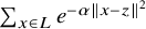
Theorem 1.1 implies that stable critical points are quite special. Candidates for stable critical points can be identified using the Delaunay decomposition. For a point to be a stable critical point, it is necessary to be the barycenter of the vertices of its Delaunay polytope, thus the barycenter of the vertices of a face of a full-dimensional Delaunay polytope. This condition does not hold for generic points, whose Delaunay polytope is $0$
-dimensional and consists only of the nearest lattice point, see Figure 1.
$0$
-dimensional and consists only of the nearest lattice point, see Figure 1.
The Delaunay decomposition of a lattice and the candidates for stable cold spots.

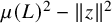
This strong condition further implies that lattices possessing stable cold spots are also quite special. Since stable cold spots can only occur at deep holes, a necessary condition for a deep hole to be a stable cold spot is that it is the barycenter of the vertices of its Delaunay polytope. This condition is not satisfied for generic lattices, see Figure 2.
Deep holes are not stable cold spots for generic lattices.

One reason why every inhomogeneous shell $L(z,r)$
could be balanced comes from central symmetry. We have
$L(z,r)$
could be balanced comes from central symmetry. We have $L(z,r) - z = -(L(z,r) - z)$
if and only if
$L(z,r) - z = -(L(z,r) - z)$
if and only if $2z$
is a lattice vector. This applies, for example, to lattice points and to midpoints of the facets of the Voronoi cell
$2z$
is a lattice vector. This applies, for example, to lattice points and to midpoints of the facets of the Voronoi cell $V(L)$
because of a famous characterisation of facet midpoints due to Voronoi [Reference Voronoi26]: a point y is a facet midpoint of
$V(L)$
because of a famous characterisation of facet midpoints due to Voronoi [Reference Voronoi26]: a point y is a facet midpoint of $V(L)$
if and only if
$V(L)$
if and only if $2y \in L$
and
$2y \in L$
and $\pm 2y$
are the unique shortest vectors in the coset
$\pm 2y$
are the unique shortest vectors in the coset $2y + 2L$
.
$2y + 2L$
.
If X is a spherical $2$
-design, we have
$2$
-design, we have
 $$\begin{align*}\sum_{x \in X} (x-z) (x-z)^{\mathsf{T}} = \frac{r^2 |X|}{n} I_n, \end{align*}$$
and therefore, when every inhomogeneous shell is a spherical $2$
-design, the Hessian simplifies to
$2$
-design, the Hessian simplifies to
 $$ \begin{align} \nabla^2 p(f, L, z) = \sum_{r \geq 0} |L(z,r)| \left(2f'(r^2) + \frac{4r^2}{n} f"(r^2) \right)I_n. \end{align} $$
1.5 Summary of the main results
The main result of this paper, proved in Section 2, is that in lattices with ‘highly symmetric’ deep holes, the deep holes are equal to cold spots for $f_{\alpha }$
when
$f_{\alpha }$
when $\alpha $
is large enough.
$\alpha $
is large enough.
Theorem 1.2. Let $L \subseteq \mathbb {R}^n$
be an n-dimensional lattice and let
$L \subseteq \mathbb {R}^n$
be an n-dimensional lattice and let $c \in \mathbb {R}^n$
be a deep hole of L. Suppose that, up to equivalence (by the affine isometry group of the lattice), c is the only deep hole of L. Suppose further that every inhomogeneous shell around c is a spherical
$c \in \mathbb {R}^n$
be a deep hole of L. Suppose that, up to equivalence (by the affine isometry group of the lattice), c is the only deep hole of L. Suppose further that every inhomogeneous shell around c is a spherical $2$
-design. Then c is a stable cold spot.
$2$
-design. Then c is a stable cold spot.
In our proof we combine two different bounds for inhomogeneous Gaussian lattice sums by a covering argument. The first bound is from Bétermin, Petrache [Reference Bétermin and Petrache7], which is helpful to bound $p(f_{\alpha },L,z)$
for points z far away from deep holes. The second bound is new and comes from an application of linear programming bounds for spherical designs. With this bound one can show that deep holes are local minimizers for
$p(f_{\alpha },L,z)$
for points z far away from deep holes. The second bound is new and comes from an application of linear programming bounds for spherical designs. With this bound one can show that deep holes are local minimizers for $z \mapsto p(f_{\alpha },L,z)$
. Furthermore, it also yields very explicit, quantitative information about the inhomogeneous Gaussian lattice sum in the neighbourhood of c, which is needed for the covering argument.
$z \mapsto p(f_{\alpha },L,z)$
. Furthermore, it also yields very explicit, quantitative information about the inhomogeneous Gaussian lattice sum in the neighbourhood of c, which is needed for the covering argument.
In Section 3 we show that our main theorem is applicable to all root lattices.
Theorem 1.3. The deep holes of root lattices are stable cold spots.
For this we determine the stabilizer subgroup of the affine isometry group of the lattice at a deep hole and see that all inhomogeneous shells around deep holes carry spherical $2$
-designs. In the situation of root lattices we can improve the generic covering argument used to prove Theorem 1.2. By this we get reasonable estimates for the threshold
$2$
-designs. In the situation of root lattices we can improve the generic covering argument used to prove Theorem 1.2. By this we get reasonable estimates for the threshold $\alpha _0$
. For example, we shall show that for
$\alpha _0$
. For example, we shall show that for $L = E_8$
already
$L = E_8$
already $\alpha _0 = 23$
suffices (Theorem 3.8) and for
$\alpha _0 = 23$
suffices (Theorem 3.8) and for $L = D_4$
already
$L = D_4$
already $\alpha _0 = 5$
suffices (Theorem 3.9).
$\alpha _0 = 5$
suffices (Theorem 3.9).
Using the same strategy we shall see in Section 4 that the dual of the exceptional root lattices $E_6^*$
,
$E_6^*$
, $E_7^*$
, as well as the Coxeter-Todd lattice in dimension
$E_7^*$
, as well as the Coxeter-Todd lattice in dimension $12$
and the Barnes-Wall lattice in dimension
$12$
and the Barnes-Wall lattice in dimension $16$
can be treated by Theorem 1.2. In all these cases the deep holes are stable cold spots.
$16$
can be treated by Theorem 1.2. In all these cases the deep holes are stable cold spots.
However, the behaviour of the Leech lattice is somewhat unexpected.
Theorem 1.4. The Leech lattice does not have stable cold spots.
To prove this, we consider the $23$
inequivalent deep holes of the Leech lattice in Section 5, determine the one to which cold spots converge when
$23$
inequivalent deep holes of the Leech lattice in Section 5, determine the one to which cold spots converge when $\alpha $
tends to infinity, and then apply Theorem 1.1.
$\alpha $
tends to infinity, and then apply Theorem 1.1.
1.6 Open questions
It would be interesting to prove or disprove in all the treated cases, whether the stable cold spots are universal cold spots. Currently, we do not know how to attack this question. It is clear that the techniques developed in this paper will not suffice, and new ideas are needed. Also we cannot resolve the cases $A_n^*$
, for
$A_n^*$
, for $n \geq 3$
, and
$n \geq 3$
, and $D_n^*$
, for
$D_n^*$
, for $n \geq 5$
. In these cases inhomogenous shells around deep holes are all spherical
$n \geq 5$
. In these cases inhomogenous shells around deep holes are all spherical $1$
-designs but not spherical
$1$
-designs but not spherical $2$
-designs.
$2$
-designs.
2 Stable cold spots and spherical
$2$
-designs: Proof of Theorem 1.2

Before going into details, we first set up notations and sketch the strategy of our proof. Let L be an n-dimensional lattice. Up to translation by lattice vectors, it is enough to consider the restriction of the function $z \mapsto p(f_\alpha , L, z)$
to the Voronoi cell
$z \mapsto p(f_\alpha , L, z)$
to the Voronoi cell $V(L)$
. Consequently, in the rest of this section, unless explicitly stated, we assume that z and c belong to
$V(L)$
. Consequently, in the rest of this section, unless explicitly stated, we assume that z and c belong to $V(L)$
, and that c is a deep hole of L. The assumptions of Theorem 1.2 ensure that all the deep holes have the same potential.
$V(L)$
, and that c is a deep hole of L. The assumptions of Theorem 1.2 ensure that all the deep holes have the same potential.
Our proof then goes in two steps. First, Theorem 2.5 shows that if every shell around c is a spherical $2$
-design, then c is a local minimizer of
$2$
-design, then c is a local minimizer of $z \mapsto p(f_\alpha , L, z)$
, and moreover we find explicit
$z \mapsto p(f_\alpha , L, z)$
, and moreover we find explicit $\alpha _c$
and
$\alpha _c$
and $R_{\alpha _c}$
such that c is the unique minimizer in the ball
$R_{\alpha _c}$
such that c is the unique minimizer in the ball $B(c,R_{\alpha _c})$
, for every
$B(c,R_{\alpha _c})$
, for every $\alpha> \alpha _c$
. This will be proven in Section 2.2, and is our main contribution in this section. Then, with Theorem 2.5, it is enough to study the potential in a ball centered at
$\alpha> \alpha _c$
. This will be proven in Section 2.2, and is our main contribution in this section. Then, with Theorem 2.5, it is enough to study the potential in a ball centered at $0$
and of radius
$0$
and of radius $\varrho < \mu (L)$
, the covering radius of L. This is the purpose of Theorem 2.1, and is a consequence of previous work by Bétermin and Petrache, that we discuss in Section 2.1.
$\varrho < \mu (L)$
, the covering radius of L. This is the purpose of Theorem 2.1, and is a consequence of previous work by Bétermin and Petrache, that we discuss in Section 2.1.
2.1 Bounding inhomogeneous Gaussian lattice sums: Far away from deep holes
We revisit some of the arguments originally due to Bétermin and Petrache [Reference Bétermin and Petrache7, Theorem 1.5], in order to obtain the following result that meets our needs:
Theorem 2.1. Let $c\in V(L)$
be a deep hole of L, and let
$c\in V(L)$
be a deep hole of L, and let $\varrho $
such that
$\varrho $
such that $\varrho < \mu (L)$
. Then there exists
$\varrho < \mu (L)$
. Then there exists $\alpha _\varrho $
such that for any
$\alpha _\varrho $
such that for any $\alpha> \alpha _\varrho $
, for every z in the ball
$\alpha> \alpha _\varrho $
, for every z in the ball $B(0, \varrho )$
,
$B(0, \varrho )$
,
 $$\begin{align*}p(f_\alpha, L, z)> p(f_\alpha, L, c). \end{align*}$$
This result is an immediate consequence of the following inequality:
Lemma 2.2. Let L be an n-dimensional lattice, let c be a deep hole of L, and let $z \in \mathbb {R}^n$
be an arbitary point. If
$z \in \mathbb {R}^n$
be an arbitary point. If $\alpha> n / (2 \mu (L)^2)$
, then
$\alpha> n / (2 \mu (L)^2)$
, then
 $$ \begin{align} \left(\sum_{x \in L} e^{-\alpha \|x-c\|^2} \right) \bigg/ \left(\sum_{x \in L} e^{-\alpha \|x-z\|^2} \right) \leq e^{-\alpha(\mu(L)^2 - \|z\|^2)} \left(\frac{2\alpha \mu(L)^2 e}{n} \right)^{n/2}. \end{align} $$
Indeed, for every z in $B(0, \varrho )$
,
$B(0, \varrho )$
,
 $$\begin{align*}\mu(L)^2 - \|z\|^2> \mu(L)^2 - \varrho^2 > 0, \end{align*}$$
and
 $$\begin{align*}e^{-\alpha(\mu(L)^2 - \varrho^2)} \left(\frac{2\alpha\mu(L)^2 e}{n} \right)^{n/2} \end{align*}$$
goes to $0$
when
$0$
when $\alpha $
tends to infinity. Note that this proof gives an explicit estimate on
$\alpha $
tends to infinity. Note that this proof gives an explicit estimate on $\alpha _\varrho $
depending on
$\alpha _\varrho $
depending on $\varrho $
.
$\varrho $
.
It remains to prove Lemma 2.2. For this, we need estimates by Banaszczyk [Reference Banaszczyk3], which in the following variant can be found in [Reference Barvinok5, Lemma 18.2 and Problem 18.4.1].
Lemma 2.3. Let L be an n-dimensional lattice. Then:
-
(a) For every
$r> \sqrt {\frac {n}{2\pi }}$
and every
$z\in \mathbb {R}^n$
,
$$\begin{align*}\sum_{x \in L, \| x - z \|> r } e^{-\pi \| x - z \|^2} \leq e^{-\pi r^2}\left(\frac{2\pi e r^2}{n}\right)^{n / 2} \sum_{x \in L} e^{-\pi \|x\|^2}. \end{align*}$$
-
(b) For every
$\alpha>0$
and every
$z\in \mathbb {R}^n$
,
$$\begin{align*}\sum_{x \in L} e^{-\alpha \|x\|^2} \leq e^{\alpha \|z\|^2} \sum_{x \in L} e^{-\alpha \|x-z\|^2}. \end{align*}$$


Proof of Lemma 2.2.
We can write
 $$\begin{align*}\sum_{x \in L} e^{-\alpha\| x - c\|^2} = \sum_{x \in \sqrt{\alpha/\pi} L} e^{-\pi \| x - \sqrt{\alpha/\pi} c\|^2}. \end{align*}$$
Now $\sqrt {\alpha /\pi } c$
is a deep hole of the scaled lattice
$\sqrt {\alpha /\pi } c$
is a deep hole of the scaled lattice $\sqrt {\alpha /\pi } L$
. For a given radius r, we can split the last sum into two parts,
$\sqrt {\alpha /\pi } L$
. For a given radius r, we can split the last sum into two parts,
 $$\begin{align*}\sum_{x \in \sqrt{\alpha/\pi } L, \| x - \sqrt{\alpha/\pi} c\| \leq r } e^{-\pi \| x - \sqrt{\alpha/\pi} c\|^2} + \sum_{x \in \sqrt{\alpha/\pi} L, \| x - \sqrt{\alpha/\pi} c\|> r } e^{-\pi \| x - \sqrt{\alpha/\pi} c\|^2}. \end{align*}$$
Observe that the first sum vanishes whenever r is strictly smaller than $\sqrt {\alpha /\pi } \mu (L)$
, the covering radius of
$\sqrt {\alpha /\pi } \mu (L)$
, the covering radius of $\sqrt {\alpha /\pi } L$
. If
$\sqrt {\alpha /\pi } L$
. If $\alpha $
is large enough, we can choose r in the range
$\alpha $
is large enough, we can choose r in the range $\sqrt {\frac {n}{2\pi }} < r < \sqrt {\alpha /\pi } \mu (L)$
so that we can apply (a) of Lemma 2.3. This gives
$\sqrt {\frac {n}{2\pi }} < r < \sqrt {\alpha /\pi } \mu (L)$
so that we can apply (a) of Lemma 2.3. This gives
 $$\begin{align*}\begin{aligned} \sum_{x \in L} e^{-\alpha \|x-c\|^2} & = \sum_{x \in \sqrt{\alpha/\pi} L, \| x - \sqrt{\alpha/\pi} c\|> r } e^{-\pi \| x - \sqrt{\alpha/\pi} c\|^2}\\ & \leq e^{-\pi r^2} \left(\frac{2 \pi e r^2}{n} \right)^{n/2} \sum_{x \in \sqrt{\alpha/\pi} L} e^{-\pi\|x\|^2}. \end{aligned} \end{align*}$$
Now we apply (b) of Lemma 2.3,
 $$\begin{align*}\sum_{x \in L} e^{-\alpha \|x-c\|^2} \leq e^{-\pi r^2} \left(\frac{2 \pi e r^2}{n} \right)^{n/2} e^{-\alpha\|z\|^2} \sum_{x \in L} e^{-\alpha\|x-z\|^2}. \end{align*}$$
By letting r tending to $\sqrt {\alpha /\pi } \mu (L)$
we get the desired inequality (2).
$\sqrt {\alpha /\pi } \mu (L)$
we get the desired inequality (2).
Based on Lemma 2.3, Bétermin and Petrache obtain the following statement [Reference Bétermin and Petrache7, Theorem 1.5], which is an immediate consequence of Theorem 2.1.
Corollary 2.4. Let L be an n-dimensional lattice and let c be a deep hole of L. Then for any $z\in \mathbb {R}^n$
, which is not a deep holeFootnote 1, there exists
$z\in \mathbb {R}^n$
, which is not a deep holeFootnote 1, there exists $\alpha _z$
such that for any
$\alpha _z$
such that for any $\alpha> \alpha _z$
,
$\alpha> \alpha _z$
,
 $$\begin{align*}p(f_\alpha, L, z)> p(f_\alpha, L, c). \end{align*}$$
Thus, for $\alpha \to \infty $
cold spots tend to deep holes.
$\alpha \to \infty $
cold spots tend to deep holes.
Note that the arguments given above are not strong enough to prove that cold spots are deep holes for finite $\alpha $
. The quantity
$\alpha $
. The quantity $\mu (L)^2 - \| z \|^2$
cannot be uniformly bounded from below with respect to z in the Voronoi cell of L.
$\mu (L)^2 - \| z \|^2$
cannot be uniformly bounded from below with respect to z in the Voronoi cell of L.
2.2 Bounding inhomogeneous Gaussian lattice sums: Using the linear programming bound for spherical designs around deep holes
Here we prove that if every shell around a deep hole is a spherical $2$
-design, then the deep hole is a (strict) local minimizer when
$2$
-design, then the deep hole is a (strict) local minimizer when $\alpha $
is large enough. That is, we show:
$\alpha $
is large enough. That is, we show:
Theorem 2.5. Let L be an n-dimensional lattice and c be a deep hole of L. Assume that all inhomogeneous shells around c are spherical $2$
-designs. Then there exist
$2$
-designs. Then there exist $\alpha _c$
and
$\alpha _c$
and $R_{\alpha _c}$
such that for every
$R_{\alpha _c}$
such that for every $\alpha \geq \alpha _c$
and for every
$\alpha \geq \alpha _c$
and for every $z\neq c$
in the ball
$z\neq c$
in the ball $B(c,R_{\alpha _c})$
, strict inequality
$B(c,R_{\alpha _c})$
, strict inequality $p(f_\alpha , L, z)> p(f_\alpha , L, c)$
holds.
$p(f_\alpha , L, z)> p(f_\alpha , L, c)$
holds.
Moreover, explicit estimates on $\alpha _c$
and
$\alpha _c$
and $R_{\alpha _c}$
will be given in Lemma 2.9.
$R_{\alpha _c}$
will be given in Lemma 2.9.
Qualitatively, it is easy to see that c is a local minimizer for $\alpha $
large enough, using the computation of the Hessian in (1), which for the Gaussian core model evaluates to
$\alpha $
large enough, using the computation of the Hessian in (1), which for the Gaussian core model evaluates to
 $$\begin{align*}\nabla^2 p(f_\alpha, L, c) = \sum_{r \geq 0} |L(c,r)| \left( \frac{4\alpha^2 r^2}{n} - 2\alpha\right) e^{-\alpha r^2} I_n. \end{align*}$$
Indeed, if $\alpha $
is sufficiently large, then all summands are positive multiples of the identity matrix. This ensures the existence of a radius
$\alpha $
is sufficiently large, then all summands are positive multiples of the identity matrix. This ensures the existence of a radius $R_\alpha>0$
such that c is a minimizer in the ball
$R_\alpha>0$
such that c is a minimizer in the ball $B(c,R_\alpha )$
.
$B(c,R_\alpha )$
.
However, as we aim to combine this local information with Theorem 2.1 to obtain a global bound, we need to derive a uniform lower bound for $R_\alpha $
when
$R_\alpha $
when $\alpha $
is large enough. The formula for the Hessian is easy to evaluate at a point z only when all inhomogeneous shells around z are spherical
$\alpha $
is large enough. The formula for the Hessian is easy to evaluate at a point z only when all inhomogeneous shells around z are spherical $2$
-designs. So information about the Hessian at points close to c seem to be difficult to get. A more delicate analysis is required.
$2$
-designs. So information about the Hessian at points close to c seem to be difficult to get. A more delicate analysis is required.
For this, we will heavily use the linear programming bound for spherical designs, originally developed by Fazekas and Levenshtein [Reference Fazekas and Levenshtein20] and Yudin [Reference Yudin27] to determine lower bounds for the covering radius of spherical designs. Later, in the context of polarization problems on spheres, this linear programming bound was modified in [Reference Boyvalenkov, Dragnev, Hardin, Saff and Stoyanova12] and [Reference Borodachov10].
Let us recall the details of this linear programming bound. Let $a : [-1,1] \to \mathbb {R}$
be any function. We are interested in determining
$a : [-1,1] \to \mathbb {R}$
be any function. We are interested in determining
 $$\begin{align*}E_a(X) = \min\left\{\sum_{x \in X} a(x \cdot y) : y \in S^{n-1}\right\}. \end{align*}$$
To state the linear programming bound for $E_a$
we need to introduce specific polynomials
$E_a$
we need to introduce specific polynomials $P^n_k$
. They are univariate polynomials of degree k, normalized by
$P^n_k$
. They are univariate polynomials of degree k, normalized by $P^n_k(1) = 1$
, and orthogonal in the following sense
$P^n_k(1) = 1$
, and orthogonal in the following sense
 $$\begin{align*}\int_{-1}^1 P^n_k(t) P^n_l(t) (1-t^2)^{(n-3)/2} dt = 0 \quad \text{ if } k \neq l. \end{align*}$$
In fact, the polynomials $P^n_k$
are appropriate multiples of the Jacobi polynomials
$P^n_k$
are appropriate multiples of the Jacobi polynomials $P^{(n-3)/2,(n-3)/2}_k$
, see for instance the book [Reference Andrews, Askey and Roy1] by Andrews, Askey, and Roy. Note that we have
$P^{(n-3)/2,(n-3)/2}_k$
, see for instance the book [Reference Andrews, Askey and Roy1] by Andrews, Askey, and Roy. Note that we have
 $$\begin{align*}P_0^n(t) = 1, \quad P_1^n(t) = t,\quad P_2^n(t) = \frac{1}{n-1}(nt^2-1). \end{align*}$$
Lemma 2.6. Let $X \subseteq S^{n-1}$
be a spherical M-design and let
$X \subseteq S^{n-1}$
be a spherical M-design and let $a : [-1, 1] \to \mathbb {R}$
be any function. Let
$a : [-1, 1] \to \mathbb {R}$
be any function. Let $h(t) = \sum _{k = 0}^M h_k P^n_k(t)$
be a polynomial so that
$h(t) = \sum _{k = 0}^M h_k P^n_k(t)$
be a polynomial so that $h(t) \leq a(t)$
for all
$h(t) \leq a(t)$
for all $t \in [-1,1]$
, then the inequality
$t \in [-1,1]$
, then the inequality $h_0 |X| \leq E_a(X)$
holds.
$h_0 |X| \leq E_a(X)$
holds.
Proof. The inequality follows easily from orthogonality and the spherical design property. For $y \in S^{n-1}$
,
$y \in S^{n-1}$
,
 $$\begin{align*}\begin{aligned} E_a(X) & \geq \sum_{x \in X} a(x \cdot y) \geq \sum_{x \in X} h(x \cdot y) = |X| \frac{1}{|X|} \sum_{x \in X} \sum_{k=0}^M h_k P_k^n(x \cdot y)\\ & = |X| \sum_{k= 0}^M h_k \int_{S^{n-1}} P_k(x \cdot y) \, d\omega(x)\\ & = |X| \sum_{k= 0}^M h_k \int_{-1}^1 P_k(t) (1-t^2)^{(n-3)/2} \, dt\\ & = |X| h_0. \end{aligned}\\[-38pt] \end{align*}$$
As usual, the proof of the previous lemma provides additional information about sharp cases; that is, when there is a polynomial h and a point $y \in S^{n-1}$
with
$y \in S^{n-1}$
with
 $$\begin{align*}h_0 |X| = E_a(X) = \sum_{x \in X} a(x \cdot y). \end{align*}$$
Indeed, one sees from the proof that this can only happen when $a(x \cdot y) = h(x \cdot y)$
for
$a(x \cdot y) = h(x \cdot y)$
for $x \in X$
. Since we also need
$x \in X$
. Since we also need $h(t) \leq a(t)$
for all
$h(t) \leq a(t)$
for all $t \in [-1,1]$
this also means that, if a is differentiable, h and a need to coincide up to second order when
$t \in [-1,1]$
this also means that, if a is differentiable, h and a need to coincide up to second order when $x \cdot y \in (-1,1)$
for
$x \cdot y \in (-1,1)$
for $x \in X$
.
$x \in X$
.
Our strategy is to bound the inhomogeneous Gaussian lattice sum close to the deep hole c using the linear programming bound for every inhomogeneous shell $L(c,r)$
and for the points on every concentric sphere
$L(c,r)$
and for the points on every concentric sphere $c + \rho y$
, with
$c + \rho y$
, with $y \in S^{n-1}$
, around the deep hole c.
$y \in S^{n-1}$
, around the deep hole c.

To bound $p(f_\alpha , L, z)$
for points z close to a deep hole c we apply the linear programming bound for every concentric sphere
$p(f_\alpha , L, z)$
for points z close to a deep hole c we apply the linear programming bound for every concentric sphere $z = c + \rho y$
, with
$z = c + \rho y$
, with $\rho> 0$
and
$\rho> 0$
and $y \in S^{n-1}$
, and for every inhomogeneous shell
$y \in S^{n-1}$
, and for every inhomogeneous shell $L(c,r)$
;
$L(c,r)$
;
 $$\begin{align*}\begin{aligned} p(L,f_\alpha, z) & = \sum_{x \in L} e^{-\alpha \|x - z\|^2} = \sum_{x \in L} e^{-\alpha\|x - c - \rho y\|^2} \\ & = \sum_{r \geq 0} e^{-\alpha r^2} e^{-\alpha \rho^2} \sum_{x \in L(c,r)} e^{2\alpha \rho r ((x-c)/r) \cdot y}; \end{aligned} \end{align*}$$
see Figure 3.
Lemma 2.7. Suppose the inhomogeneous shell $L(c,r)$
is a spherical
$L(c,r)$
is a spherical $2$
-design. Then
$2$
-design. Then
 $$ \begin{align} \sum_{x \in L(c,r)} e^{2\alpha \rho r ((x-c)/r) \cdot y} \geq |L(c,r)| b(\alpha, \rho, r) \end{align} $$
holds with
 $$\begin{align*}b(\alpha, \rho, r) = \frac{ne^{\frac{2\alpha \rho r}{n}}+e^{-2\alpha \rho r}}{n+1}, \end{align*}$$
and if $L(c,r)$
is additionally centrally symmetric, then
$L(c,r)$
is additionally centrally symmetric, then
 $$\begin{align*}b(\alpha, \rho, r) = \cosh\left(\frac{2\alpha \rho r}{\sqrt{n}}\right). \end{align*}$$
Proof.
-
1. We apply Lemma 2.6 to
$X = \{ \frac {x-c}{r} : x\in L(c,r)\}$
, and functions
$a(t)$
of the form Then a feasible solution for Lemma 2.6 is given by:
$$\begin{align*}a_\gamma(t) = \exp(\gamma t) \quad \text{with } \gamma = 2\alpha \rho r. \end{align*}$$
with
$$\begin{align*}h_\gamma(t) = h_0P_0^n(t) + h_1P_1^n(t) + h_2P_2^n(t) \end{align*}$$
The polynomial h interpolates the function
$$ \begin{align*} h_0 &= \frac{ne^{\frac{\gamma}{n}}+e^{-\gamma}}{n+1} \\ h_1 &= \frac{(\gamma n^2 - \gamma +2n)e^{\frac{\gamma}{n}}-2ne^{-\gamma}}{(n+1)^2} \\ h_2 &= \frac{((\gamma-1)n^2 - \gamma + n )e^{\frac{\gamma}{n}}+ n(n-1) e^{-\gamma}}{(n+1)^2}. \end{align*} $$
$a_\gamma (t)$
at the points
$t = -1$
with multiplicity
$1$
, and
$t = 1/n$
with multiplicity
$2$
. By applying Lemma 2.1 from [Reference Cohn and Kumar14], we have
$h_\gamma (t) \leq \exp (\gamma t)$
on
$[-1,1]$
.
-
2. Because the inhomogeneous shell
$L(c,r)$
is centrally symmetric we can rewrite the sum We apply Lemma 2.6 to functions
$$\begin{align*}\sum_{x \in L(c,r)} e^{2\alpha \rho r ((x-c)/r) \cdot y} = \sum_{x \in L(c,r)} \cosh(2 \alpha \rho r ((x-c)/r) \cdot y). \end{align*}$$
$a(t)$
of the form Then a feasible solution for Lemma 2.6 is given by:
$$\begin{align*}a_\gamma(t) = \cosh(\gamma t) \quad \text{with } \gamma = 2\alpha \rho r. \end{align*}$$
Now that
$$\begin{align*}h_\gamma(t) = \cosh\left(\frac{\gamma}{\sqrt{n}}\right) P_0^n(t) + \frac{\gamma}{2}\sinh\left(\frac{\gamma}{\sqrt{n}}\right)\frac{n-1}{\sqrt{n}}P_2^n(t). \end{align*}$$
$a_\gamma $
is even, we may assume that
$h_\gamma $
is even. This leaves freedom only to the coefficients
$h_0$
and
$h_2$
. We use Hermite interpolation at
$t=\frac {1}{\sqrt {n}}$
at order
$2$
, and apply again [Reference Cohn and Kumar14, Lemma 2.1] to show
$h_\gamma (t) \leq \exp (\gamma t)$
on
$[-1,1]$
.


Remark 2.8. The bounds of the previous lemma are in fact optimal.
In the first case, the bound is tight, when X are the vertices of a regular simplex and when $y = - v$
, where v is any vertex of the simplex. Then the inner products between y and the elements of X are the interpolation points
$y = - v$
, where v is any vertex of the simplex. Then the inner products between y and the elements of X are the interpolation points $-1$
and
$-1$
and $1/n$
. Therefore,
$1/n$
. Therefore,
 $$\begin{align*}E_{a_\gamma}(X) \leq \sum_{x\in X} a_\gamma (x \cdot y) = \sum_{x\in X} h_\gamma (x \cdot y) = h_0 |X| \leq E_{a_\gamma}(X), \end{align*}$$
which shows the optimality of the bound.
In the second case, the bound is tight when X are the vertices of a cross polytope, namely $X=\{\pm e_i\}$
, where
$X=\{\pm e_i\}$
, where $e_i$
is the i-th vector of the canonical basis. For
$e_i$
is the i-th vector of the canonical basis. For $y = \frac {1}{\sqrt {n}} \sum _{i = 1}^n e_i$
, then the inner products between y and the elements of X are the interpolation points
$y = \frac {1}{\sqrt {n}} \sum _{i = 1}^n e_i$
, then the inner products between y and the elements of X are the interpolation points $\pm \frac {1}{\sqrt {n}}$
, which proves optimality.
$\pm \frac {1}{\sqrt {n}}$
, which proves optimality.
With Lemma 2.7, we have
 $$\begin{align*}p(L,f_\alpha, z) \geq \sum_{r \geq 0} |L(c,r)| e^{-\alpha r^2} e^{-\alpha \rho^2} b(\alpha, \rho, r). \end{align*}$$
On the other hand,
 $$\begin{align*}p(f_\alpha, L, c) = \sum_{r \geq 0} |L(c,r)| e^{-\alpha r^2}. \end{align*}$$
Thus, if for a given $\alpha $
, we find R such that for every
$\alpha $
, we find R such that for every $0< \rho < R$
, and for every r the strict inequality
$0< \rho < R$
, and for every r the strict inequality
 $$ \begin{align} e^{-\alpha \rho^2} b(\alpha,\rho,r)> 1 \end{align} $$
holds, then we get that for every $z\neq c$
in the ball
$z\neq c$
in the ball $B(c,R)$
,
$B(c,R)$
,
 $$\begin{align*}p(f_\alpha, L, z) - p(f_\alpha, L, c) \geq \sum_{r \geq 0} |L(c,r)| e^{-\alpha r^2} (e^{-\alpha \rho^2} b(\alpha,\rho,r) - 1)> 0. \end{align*}$$
We need to verify inequality (4). Note that since both expressions $b(\alpha , \rho , r)$
are increasing with r, if (4) is satisfied for
$b(\alpha , \rho , r)$
are increasing with r, if (4) is satisfied for $r = \mu (L)$
, then it is satisfied for every
$r = \mu (L)$
, then it is satisfied for every $r \geq \mu (L)$
.
$r \geq \mu (L)$
.
We therefore consider the function
 $$\begin{align*}g(\rho) = e^{-\alpha \rho^2}b(\alpha,\rho,\mu(L)) - 1, \end{align*}$$
and look for $R_\alpha>0$
such that for every
$R_\alpha>0$
such that for every $0 < \rho < R_\alpha $
,
$0 < \rho < R_\alpha $
, $g(\rho )>0$
.
$g(\rho )>0$
.
Lemma 2.9. In the general case, when the inhomogeneous shells are spherical 2-designs, then for every $\alpha $
such that
$\alpha $
such that $\alpha> \frac {n^2}{ \mu (L)^2}(\frac {n+1}{2n} + \log (\frac {n+1}{n})^2)$
, then
$\alpha> \frac {n^2}{ \mu (L)^2}(\frac {n+1}{2n} + \log (\frac {n+1}{n})^2)$
, then $g(\rho )> 0$
on the interval
$g(\rho )> 0$
on the interval $\left (0, R_\alpha \right ]$
, where
$\left (0, R_\alpha \right ]$
, where
 $$\begin{align*}R_\alpha = \frac{\mu(L)}{n} + \sqrt{\frac{\mu(L)^2}{n^2}- \frac{\log(\frac{n+1}{n})}{\alpha}}. \end{align*}$$
When, moreover, the inhomogeneous shells are centrally symmetric, then the inequality $\alpha> \frac {n}{ \mu (L)^2}(1/2 + \log (2)^2)$
is sufficient, and we can take
$\alpha> \frac {n}{ \mu (L)^2}(1/2 + \log (2)^2)$
is sufficient, and we can take
 $$\begin{align*}R_\alpha = \frac{\mu(L)}{\sqrt{n}} + \sqrt{\frac{\mu(L)^2}{n}- \frac{\log(2)}{\alpha}}. \end{align*}$$
Proof. We focus on the general case where
 $$\begin{align*}g(\rho) = e^{-\alpha \rho^2}\left(\frac{ne^{\frac{2\alpha \rho \mu(L)}{n}}+e^{-2\alpha \rho \mu(L)}}{n+1}\right) - 1, \end{align*}$$
because the second, more specific case, is similar. The strategy consists in using two different estimates: a first one to ensure the positivity of $g(\rho )$
for
$g(\rho )$
for $\rho $
in an interval of the form
$\rho $
in an interval of the form $[r_\alpha , R_\alpha ]$
, and second one, using the Taylor expansion of g around
$[r_\alpha , R_\alpha ]$
, and second one, using the Taylor expansion of g around $0$
, to make sure that
$0$
, to make sure that $g(\rho )>0$
for
$g(\rho )>0$
for $\rho \in (0,r_\alpha )$
.
$\rho \in (0,r_\alpha )$
.
First, we use the trivial lower bound
 $$\begin{align*}\frac{ne^{\frac{2\alpha \rho \mu(L)}{n}}+e^{-2\alpha \rho \mu(L)}}{n+1}> \frac{ne^{\frac{2\alpha \mu(L) \rho}{{n}}}}{n+1}, \end{align*}$$
which gives
 $$\begin{align*}g(\rho)> \frac{ne^{\alpha \rho\left(\frac{2\mu(L)}{n}-\rho\right)}-(n+1)}{n+1} \end{align*}$$
and therefore $g(\rho )>0$
whenever
$g(\rho )>0$
whenever
 $$\begin{align*}\alpha \rho\left(\frac{2\mu(L)}{n}-\rho\right)> \log\left(\frac{n+1}{n}\right). \end{align*}$$
Because $\frac {n+1}{2n} + \log \left (\frac {n+1}{n}\right )^2> \log \left (\frac {n+1}{n}\right )$
, the assumption on
$\frac {n+1}{2n} + \log \left (\frac {n+1}{n}\right )^2> \log \left (\frac {n+1}{n}\right )$
, the assumption on $\alpha $
ensures that
$\alpha $
ensures that $g(\rho )>0$
on the interval
$g(\rho )>0$
on the interval
 $$\begin{align*}\left[ \frac{\mu(L)}{{n}} - \sqrt{\frac{\mu(L)^2}{n^2} - \frac{\log\left(\frac{n+1}{n}\right)}{\alpha}}, \frac{\mu(L)}{{n}} + \sqrt{\frac{\mu(L)^2}{n^2} - \frac{\log\left(\frac{n+1}{n}\right)}{\alpha}} \right] .\end{align*}$$
It remains to deal with small $\rho $
. Note that because
$\rho $
. Note that because $\sqrt {1-x} \geq 1-x$
for every
$\sqrt {1-x} \geq 1-x$
for every $0\leq x \leq 1$
, we have
$0\leq x \leq 1$
, we have
 $$\begin{align*}\frac{\mu(L)}{n} - \sqrt{\frac{\mu(L)^2}{n^2} - \frac{\log\left(\frac{n+1}{n}\right)}{\alpha}} = \frac{\mu(L)}{n} - \frac{\mu(L)}{n}\sqrt{1 - \frac{\log\left(\frac{n+1}{n}\right)n^2}{\alpha\mu(L)^2}} \leq \frac{\log\left(\frac{n+1}{n}\right){n}}{\alpha\mu(L)} \end{align*}$$
and therefore it is sufficient to prove that $g(\rho )>0$
on
$g(\rho )>0$
on $\left (0,\frac {\log \left (\frac {n+1}{n}\right ){n}}{\alpha \mu (L)} \right ]$
. For
$\left (0,\frac {\log \left (\frac {n+1}{n}\right ){n}}{\alpha \mu (L)} \right ]$
. For $\rho $
in this interval, we have
$\rho $
in this interval, we have
 $$\begin{align*}e^{-\alpha \rho^2} \geq 1 -\alpha \rho^2> 0. \end{align*}$$
Moreover, since
 $$\begin{align*}e^{\frac{2\alpha \rho \mu(L)}{n}}> 1 + \frac{2\alpha \rho \mu(L)}{n} + \frac{2\alpha^2 \rho^2 \mu(L)^2}{n^2} \end{align*}$$
and
 $$\begin{align*}e^{-2\alpha \rho \mu(L)}> 1 - 2\alpha \rho \mu(L), \end{align*}$$
then
 $$\begin{align*}ne^{\frac{2\alpha \rho \mu(L)}{n}}+e^{-2\alpha \rho \mu(L)}> n+1 + \frac{2\alpha^2 \rho^2 \mu(L)^2}{n}. \end{align*}$$
We get
 $$\begin{align*}g(\rho)> (1 -\alpha \rho^2)\left(1 + \frac{2\alpha^2 \mu(L)^2 \rho^2}{n(n+1)}\right) - 1 = -\alpha \rho^2\left( 1 - \frac{2\alpha \mu(L)^2}{n(n+1)} + \frac{2\alpha^2 \mu(L)^2 \rho^2}{n(n+1)} \right), \end{align*}$$
which is positive between $0$
and
$0$
and
 $$\begin{align*}\sqrt{\frac{1}{\alpha} - \frac{n(n+1)}{2\alpha^2 \mu(L)^2}} = \sqrt{\frac{\alpha - \frac{n(n+1)}{2\mu(L)^2}}{\alpha^2}}. \end{align*}$$
Thus $g(\rho )> 0$
on
$g(\rho )> 0$
on $\left (0,\frac {\log \left (\frac {n+1}{n}\right ){n}}{\alpha \mu (L)} \right ]$
whenever
$\left (0,\frac {\log \left (\frac {n+1}{n}\right ){n}}{\alpha \mu (L)} \right ]$
whenever $\alpha - \frac {n(n+1)}{2\mu (L)^2}> \frac {\log \left (\frac {n+1}{n}\right )^2n^2}{\mu (L)^2}$
, which is ensured by the assumption on
$\alpha - \frac {n(n+1)}{2\mu (L)^2}> \frac {\log \left (\frac {n+1}{n}\right )^2n^2}{\mu (L)^2}$
, which is ensured by the assumption on $\alpha $
.
$\alpha $
.
For the second case, we use the similar estimates
 $$\begin{align*}\cosh\left(\frac{2\alpha \mu(L) \rho}{\sqrt{n}}\right)> \frac{e^{\frac{2\alpha \mu(L) r}{\sqrt{n}}}}{2}, \end{align*}$$
and
 $$\begin{align*}g(\rho)> (1 -\alpha \rho^2)\left(1 + \frac{2\alpha^2 \mu(L)^2 \rho^2}{n}\right) - 1 = -\alpha \rho^2\left( 1 - \frac{2\alpha \mu(L)^2}{n} + \frac{2\alpha^2 \mu(L)^2 \rho^2}{n} \right).\\[-34pt] \end{align*}$$
From Lemma 2.9, we can easily deduce Theorem 2.5:
Proof of Theorem 2.5.
In the general case (respectively the centrally symmetric case), we can take any $\alpha _c> \frac {n^2}{ \mu (L)^2}(\frac {n+1}{2n} + \log (\frac {n+1}{n})^2)$
(respectively
$\alpha _c> \frac {n^2}{ \mu (L)^2}(\frac {n+1}{2n} + \log (\frac {n+1}{n})^2)$
(respectively $\alpha _c> \frac {n}{ \mu (L)^2}(1/2 + \log (2)^2)$
). Then, because the function
$\alpha _c> \frac {n}{ \mu (L)^2}(1/2 + \log (2)^2)$
). Then, because the function $\alpha \mapsto R_\alpha $
is increasing with
$\alpha \mapsto R_\alpha $
is increasing with $\alpha $
, c is the unique minimizer of
$\alpha $
, c is the unique minimizer of $z\mapsto p(f_\alpha ,L,z)$
in the ball
$z\mapsto p(f_\alpha ,L,z)$
in the ball $B(c,R_{\alpha _c})$
, for every
$B(c,R_{\alpha _c})$
, for every $\alpha \geq \alpha _c$
.
$\alpha \geq \alpha _c$
.
2.3 Putting the two bounds together, finishing the proof of Theorem 1.2
The assumptions of Theorem 1.2 allow us to apply Theorem 2.5. We have for every $\alpha \geq \alpha _c$
and for every
$\alpha \geq \alpha _c$
and for every $z \neq c$
in the ball
$z \neq c$
in the ball $B(c,R_{\alpha _c})$
,
$B(c,R_{\alpha _c})$
,
 $$\begin{align*}p(f_\alpha, L, z)> p(f_\alpha, L, c). \end{align*}$$
Since the deep holes of L are precisely the points in $V(L)$
having norm
$V(L)$
having norm $\mu (L)$
, there exists
$\mu (L)$
, there exists $0 < \varrho < \mu (L)$
such that
$0 < \varrho < \mu (L)$
such that
 $$\begin{align*}V(L) \setminus \bigcup_{c} B(c, R_{\alpha_c}) \subseteq B(0, \varrho), \end{align*}$$
where the union is taken over all the deep holes in $V(L)$
. Figure 4 illustrates this covering argument.
$V(L)$
. Figure 4 illustrates this covering argument.
Covering $V(L)$
by balls of two kinds.
$V(L)$
by balls of two kinds.

We can now apply Theorem 2.1, which provides $\alpha _\varrho $
such that for every
$\alpha _\varrho $
such that for every $\alpha> \alpha _\varrho $
and every
$\alpha> \alpha _\varrho $
and every $z \in B(0, \varrho )$
,
$z \in B(0, \varrho )$
,
 $$\begin{align*}p(f_\alpha, L, z)> p(f_\alpha, L, c). \end{align*}$$
The desired result then follows by taking $\alpha _0 = \max \{\alpha _c, \alpha _\varrho \}$
.
$\alpha _0 = \max \{\alpha _c, \alpha _\varrho \}$
.
3 Cold spots of root lattices
We now move to prepare the proof of Theorem 1.3, asserting that for large enough $\alpha $
the cold spots of a root lattice are equal to its deep holes.
$\alpha $
the cold spots of a root lattice are equal to its deep holes.
For this we firstly discuss how inhomogeneous energy behaves if a lattice is decomposable, that is, an orthogonal sum of sublattices. This allows us to restrict all investigations to indecomposable root lattices, about which we collect some basic facts in Section 3.2 and Appendix A.
In lieu of Theorem 1.2 we then only need to show that for an indecomposable root lattice L and a deep hole c of L the inhomogeneous shells
 $$\begin{align*}L(c,r) = \{x \in L : \|x-c\| = r\} \end{align*}$$
form spherical $2$
-designs whenever they are nonempty. This will be achieved in Theorem 3.3 and is based on the fact that the stabilizer group of c contains a Weyl group which induces the necessary design strength.
$2$
-designs whenever they are nonempty. This will be achieved in Theorem 3.3 and is based on the fact that the stabilizer group of c contains a Weyl group which induces the necessary design strength.
While, for the present application, it is sufficient that the stabilizer group of the deep hole c contains a suitable Weyl group, we can give a more precise characterisation of the stabilizer group, which we present in Lemma 3.6.
We conclude the section by illustrating how to compute an explicit $\alpha _0$
for the application of Theorem 1.2. We do this for the root lattices
$\alpha _0$
for the application of Theorem 1.2. We do this for the root lattices $D_4$
and
$D_4$
and $E_8$
in Theorem 3.9 and Theorem 3.8.
$E_8$
in Theorem 3.9 and Theorem 3.8.
3.1 Decomposable lattices
We will call a lattice L in $\mathbb {R}^n$
decomposable if we can find non trivial sublattices
$\mathbb {R}^n$
decomposable if we can find non trivial sublattices $L_1$
on
$L_1$
on $V_1 = \mathbb {R} L_1$
and
$V_1 = \mathbb {R} L_1$
and $L_2$
on
$L_2$
on $V_2 = \mathbb {R} L_2$
with
$V_2 = \mathbb {R} L_2$
with
 $$\begin{align*}L = L_1 \perp L_2, \end{align*}$$
otherwise L is called indecomposable. A general feature of decomposable lattices is that (inhomogeneous) energy factors multiplicatively through the orthogonal summands.
Lemma 3.1. Let $L\subset \mathbb {R}^n$
be a lattice that can be decomposed as the orthogonal direct sum of lattices
$L\subset \mathbb {R}^n$
be a lattice that can be decomposed as the orthogonal direct sum of lattices
 $$\begin{align*}L = L_1 \perp L_2 \perp \ldots \perp L_m, \end{align*}$$
namely there are subspaces $V_1, \ldots , V_m \subset \mathbb {R}^n$
such that
$V_1, \ldots , V_m \subset \mathbb {R}^n$
such that $L_i$
is a lattice in
$L_i$
is a lattice in $V_i$
for every
$V_i$
for every $1 \leq i \leq m$
, and
$1 \leq i \leq m$
, and $\mathbb {R}^n = V_1 \perp V_2 \perp \ldots \perp V_m$
. Then for any
$\mathbb {R}^n = V_1 \perp V_2 \perp \ldots \perp V_m$
. Then for any $\alpha> 0$
and
$\alpha> 0$
and $z = z_1 + \ldots + z_m$
with
$z = z_1 + \ldots + z_m$
with $z_i \in V_i$
, we have
$z_i \in V_i$
, we have
 $$\begin{align*}p(f_\alpha, L, z) = p(f_\alpha, L_1, z_1)p(f_\alpha, L_2, z_2) \cdots p(f_\alpha, L_m, z_m). \end{align*}$$
In particular, if for every $1 \leq i \leq m$
,
$1 \leq i \leq m$
, $c_i$
is a minimizer of
$c_i$
is a minimizer of $z_i \mapsto p(f_\alpha , L_i, z_i)$
, then
$z_i \mapsto p(f_\alpha , L_i, z_i)$
, then $c = c_1 + \ldots + c_m$
is a minimizer of
$c = c_1 + \ldots + c_m$
is a minimizer of $z \mapsto p(f_\alpha , L, z)$
.
$z \mapsto p(f_\alpha , L, z)$
.
Proof. It is enough to prove the statement when $L = L_1 \perp L_2$
. Then, for
$L = L_1 \perp L_2$
. Then, for $z = z_1 + z_2$
, we have
$z = z_1 + z_2$
, we have
 $$ \begin{align*} p(f_\alpha, L, z) & = \sum_{\ell \in L}e^{-\pi\alpha \| \ell - z\|^2} \\ & = \sum_{\ell_1 \in L_1, \ell_2 \in L_2}e^{-\pi\alpha \| \ell_1 + \ell_2 - z_1 - z_2\|^2} \\ & = \sum_{\ell_1 \in L_1, \ell_2 \in L_2}e^{-\pi\alpha \| \ell_1 - z_1 \|^2}e^{-\pi\alpha \| \ell_2 - z_2\|^2} \\ & = \left(\sum_{\ell_1 \in L_1}e^{-\pi\alpha \| \ell_1 - z_1 \|^2}\right)\left(\sum_{\ell_2 \in L_2}e^{-\pi\alpha \| \ell_2 - z_2\|^2}\right) \\ & = p(f_\alpha, L_1, z_1)p(f_\alpha, L_2, z_2).\\[-34pt] \end{align*} $$
3.2 Designs on inhomogeneous shells of indecomposable root lattices
An integral lattice L is a root lattice if and only if
 $$ \begin{align} L = \langle L(2) \rangle_{\mathbb{Z}}, \end{align} $$
that is, if L is generated by its elements of squared norm $2$
, which in fact is a root system. Note that as a direct consequence of the definition all root lattices are even, that is
$2$
, which in fact is a root system. Note that as a direct consequence of the definition all root lattices are even, that is $\|v\|^2 \in 2\mathbb {Z}$
for all
$\|v\|^2 \in 2\mathbb {Z}$
for all $v \in L$
.
$v \in L$
.
If L is decomposable, say $L = L_1 \perp \ldots \perp L_m$
with
$L = L_1 \perp \ldots \perp L_m$
with $L_1,\ldots ,L_m$
indecomposable, then this is true for the root system
$L_1,\ldots ,L_m$
indecomposable, then this is true for the root system
 $$\begin{align*}L(2) = L_1(2) \perp \ldots \perp L_m(2). \end{align*}$$
It is well known that in this case each root system $L_i(2)$
is indecomposableFootnote 2 as a root system and is of type
$L_i(2)$
is indecomposableFootnote 2 as a root system and is of type $A_n$
(
$A_n$
( $n \geq 2$
),
$n \geq 2$
), $D_n$
(
$D_n$
( $n \geq 3$
) or
$n \geq 3$
) or $E_n$
(
$E_n$
( $n \in \left \{ 6,7,8 \right \}$
) (c.f. [Reference Ebeling19, Theorem 1.2]).
$n \in \left \{ 6,7,8 \right \}$
) (c.f. [Reference Ebeling19, Theorem 1.2]).
For a root lattice L we write $W(L)$
for its Weyl group, which is the Weyl group of the root system
$W(L)$
for its Weyl group, which is the Weyl group of the root system $R=L(2)$
(c.f. Appendix B). Of course
$R=L(2)$
(c.f. Appendix B). Of course $W(L)$
is a subgroup of
$W(L)$
is a subgroup of $\operatorname {\mathrm {O}}(L)$
. Similarly we will write
$\operatorname {\mathrm {O}}(L)$
. Similarly we will write $W^a(L)$
for the affine Weyl group of L, which is the semi-direct product
$W^a(L)$
for the affine Weyl group of L, which is the semi-direct product
 $$\begin{align*}W^a(L) = W(L) \rtimes L \subseteq \operatorname{\mathrm{Iso}}(L) = \operatorname{\mathrm{O}}(L) \rtimes L, \end{align*}$$
where L acts on itself by translations and $\operatorname {\mathrm {Iso}}(L)$
is the affine isometry group of L.
$\operatorname {\mathrm {Iso}}(L)$
is the affine isometry group of L.
A very nice property of these root systems of type $A_n$
,
$A_n$
, $D_n$
and
$D_n$
and $E_n$
is that they are self-dual, that is
$E_n$
is that they are self-dual, that is
 $$\begin{align*}A_n = (A_n)^\vee, D_n = (D_n)^\vee, \text{ and } E_n = (E_n)^\vee. \end{align*}$$
So, in particular, if $R = L(2)$
, then
$R = L(2)$
, then $R = R^{\vee }$
(c.f. Appendix B for reference).
$R = R^{\vee }$
(c.f. Appendix B for reference).
From the above discussion we collect information on special points of root lattices, that is points in space which are stabilized by a suitably nice group of affine isometries of the lattice. It turns out that these are precisely the points of the dual of L, which, in general, is the lattice
 $$\begin{align*}L^* = \left\{ x \in \mathbb{R}^n : x \cdot v \in \mathbb{Z} \text{ for all } v \in L \right\}. \end{align*}$$
Lemma 3.2. Let L be an n-dimensional root lattice with root system $R = L(2)$
and Weyl group
$R = L(2)$
and Weyl group $W(L)$
. For
$W(L)$
. For $z \in \mathbb {R}^n$
we have
$z \in \mathbb {R}^n$
we have
 $$\begin{align*}W^a_z(L) \cong W(L) \quad \Longleftrightarrow \quad z \in L^*. \end{align*}$$
Proof. This is based on the more general concept of special points for Weyl groups, on which we collect some information in Appendix B but in general we refer to [Reference Bourbaki13].
Explicitly we note that for a point z the isomorphism $W^a_z(L) \cong W(L)$
is equivalent to z being a special point of
$W^a_z(L) \cong W(L)$
is equivalent to z being a special point of $W^a(L)$
([Reference Bourbaki13, Ch. V, §3, Proposition 9]) and the special points of root lattices are precisely the elements of the weight lattice
$W^a(L)$
([Reference Bourbaki13, Ch. V, §3, Proposition 9]) and the special points of root lattices are precisely the elements of the weight lattice $L^*$
([Reference Bourbaki13, Ch.VI, §2, Proposition 3]).
$L^*$
([Reference Bourbaki13, Ch.VI, §2, Proposition 3]).
It is the unimodularity of $E_8$
, that is,
$E_8$
, that is, $E_8 = E_8^*$
, that keeps us from including it in the framework used in Lemma 3.2. In particular we already see that special points for
$E_8 = E_8^*$
, that keeps us from including it in the framework used in Lemma 3.2. In particular we already see that special points for $E_8$
which are not lattice elements will have a stabilizer that is smaller than
$E_8$
which are not lattice elements will have a stabilizer that is smaller than $W(E_8)$
, we will adress this case in Lemma 3.6.
$W(E_8)$
, we will adress this case in Lemma 3.6.
For the subsequent discussion we need some facts about these lattices, which we collect in Table 1. In particular we emphasise that for indecomposable root lattices not of type $E_8$
all deep holes are elements of the associated dual lattice and therefore special points for the associated affine Weyl group. To justify the contents of this table we refer to Appendix A and more generally to [Reference Conway and Sloane15, Chapter 4].
$E_8$
all deep holes are elements of the associated dual lattice and therefore special points for the associated affine Weyl group. To justify the contents of this table we refer to Appendix A and more generally to [Reference Conway and Sloane15, Chapter 4].
Data regarding indecomposable root lattices.

With this we are ready to discuss the main result of this section.
Theorem 3.3. Let $L\subseteq \mathbb {R}^n$
be a root lattice and
$L\subseteq \mathbb {R}^n$
be a root lattice and $c \in \mathbb {R}^n$
a deep hole of L. Then for
$c \in \mathbb {R}^n$
a deep hole of L. Then for $r> 0$
the inhomogeneous shell
$r> 0$
the inhomogeneous shell $L(z,r)$
is either empty or a spherical
$L(z,r)$
is either empty or a spherical $2$
-design.
$2$
-design.
Proof. We can assume that L is an indecomposable root lattice, as every decomposable root lattice splits orthogonally into an orthogonal sum of indecomposable root lattices.
The main tool we use is Theorem 3.12 in [Reference Goethals and Seidel21], which states that for any finite subgroup G of the orthogonal group $\operatorname {\mathrm {O}}(\mathbb {R}^n)$
the following conditions are equivalent
$\operatorname {\mathrm {O}}(\mathbb {R}^n)$
the following conditions are equivalent
-
1. every G-orbit is a spherical t-design;
-
2. there are no G-invariant harmonic polynomials of degrees
$1,2,\ldots ,t$
.

For each irreducible root lattice we find a suitable group G which satisfies (2) with $t=2$
above and has the property that each shell
$t=2$
above and has the property that each shell $L(c,r)$
is a union of orbits of G. Then each orbit is a spherical
$L(c,r)$
is a union of orbits of G. Then each orbit is a spherical $2$
-design and so this true for
$2$
-design and so this true for $L(c,r)$
.
$L(c,r)$
.
Let c be a deep hole of L and r such that $L(c,r)$
is nonempty. Let
$L(c,r)$
is nonempty. Let $\operatorname {\mathrm {Iso}}(L)_c$
be the stabilizer of c in
$\operatorname {\mathrm {Iso}}(L)_c$
be the stabilizer of c in $\operatorname {\mathrm {Iso}}(L)$
. By Lemma 3.2 we have that if
$\operatorname {\mathrm {Iso}}(L)$
. By Lemma 3.2 we have that if $L \not \cong E_8$
, then the stabilizer of a deep hole c of L in
$L \not \cong E_8$
, then the stabilizer of a deep hole c of L in $W^a(L) \subseteq \operatorname {\mathrm {Iso}}(L)$
containsFootnote 3 (an isomorphic copy G of) the Weyl group
$W^a(L) \subseteq \operatorname {\mathrm {Iso}}(L)$
containsFootnote 3 (an isomorphic copy G of) the Weyl group $W(L)$
of L.
$W(L)$
of L.
For $L \cong E_8$
we find that there is
$L \cong E_8$
we find that there is $G \subseteq \operatorname {\mathrm {Iso}}(L)_c$
, with
$G \subseteq \operatorname {\mathrm {Iso}}(L)_c$
, with $G \cong W(D_8)$
, this can be checked by explicit computation. In fact
$G \cong W(D_8)$
, this can be checked by explicit computation. In fact $\operatorname {\mathrm {Iso}}(L)_c \cong W(D_8)$
, we prove this in Lemma 3.6 (3).
$\operatorname {\mathrm {Iso}}(L)_c \cong W(D_8)$
, we prove this in Lemma 3.6 (3).
So in all cases G can be chosen to be a Weyl group of type A, D, or E of full dimension with respect to L. Note that G is a group of isometries fixing c and therefore also fixes $L(c,r)$
set-wise, so
$L(c,r)$
set-wise, so $L(c,r)$
is indeed a union of orbits of G.
$L(c,r)$
is indeed a union of orbits of G.
We can apply [Reference Goethals and Seidel21, Theorem 3.12] to these groups, since in all cases such a Weyl group has no harmonic invariants of degree $1$
or
$1$
or $2$
. This follows from [Reference Goethals and Seidel21, Theorem 4.6], the succeeding discussion and the data in Table 1 of [Reference Goethals and Seidel21].
$2$
. This follows from [Reference Goethals and Seidel21, Theorem 4.6], the succeeding discussion and the data in Table 1 of [Reference Goethals and Seidel21].
For all root lattices which are not of type $E_8$
the proof of the above Theorem extends naturally to all special points in Table 1.
$E_8$
the proof of the above Theorem extends naturally to all special points in Table 1.
Corollary 3.4. Let $L \not \cong E_8$
be an irreducible root lattice and let c be a hole of L. Then
$L \not \cong E_8$
be an irreducible root lattice and let c be a hole of L. Then $L(c,r)$
is either empty or a spherical
$L(c,r)$
is either empty or a spherical $2$
-design.
$2$
-design.
3.3 The full stabilizer group for special points and indecomposable root lattices
The proof of Theorem 3.3 relies only on the fact that for root lattices the full stabilizer subgroup of a deep hole contains a Weyl group. We proved the existence of such a subgroup in Lemma 3.2 for all cases except $E_8$
, this case we will handle now. Along with that we compute the full stabilizer subgroups of deep holes in the affine isometry group of indecomposable root lattices. This is achieved in Lemma 3.6. While this is not necessary for the proof of Theorem 3.3 we are not aware of a reference to this problem in the literature, and it seems to be an obvious question how far the full stabilizer of a deep hole in a (indecomposable) root lattice is away from the subgroup identified in Lemma 3.2.
$E_8$
, this case we will handle now. Along with that we compute the full stabilizer subgroups of deep holes in the affine isometry group of indecomposable root lattices. This is achieved in Lemma 3.6. While this is not necessary for the proof of Theorem 3.3 we are not aware of a reference to this problem in the literature, and it seems to be an obvious question how far the full stabilizer of a deep hole in a (indecomposable) root lattice is away from the subgroup identified in Lemma 3.2.
Let $\operatorname {\mathrm {Iso}}(L)$
be the group of affine isometries of L. Every element in
$\operatorname {\mathrm {Iso}}(L)$
be the group of affine isometries of L. Every element in $\operatorname {\mathrm {Iso}}(L)$
can be written as the composition of an element
$\operatorname {\mathrm {Iso}}(L)$
can be written as the composition of an element $f\in \operatorname {\mathrm {O}}(L)$
by a translation
$f\in \operatorname {\mathrm {O}}(L)$
by a translation $t_u$
by a vector of
$t_u$
by a vector of $u\in L$
. Recall that for
$u\in L$
. Recall that for $c\in \mathbb {R}^n$
 $$\begin{align*}\operatorname{\mathrm{Iso}}(L)_c = \left\{ \phi \in \operatorname{\mathrm{Iso}}(L) : \phi(c) = c \right\} \subseteq \operatorname{\mathrm{Iso}}(L) \end{align*}$$
be the stabilizer of c in $\operatorname {\mathrm {Iso}}(L)$
.
$\operatorname {\mathrm {Iso}}(L)$
.
Firstly, we determine how the translational part and the linear part of an affine isometry $\phi $
are related if
$\phi $
are related if $\phi $
is in the stabilizer
$\phi $
is in the stabilizer $\operatorname {\mathrm {Iso}}(L)_c$
of a point c.
$\operatorname {\mathrm {Iso}}(L)_c$
of a point c.
Lemma 3.5. Let $\phi = t_u \circ f \in \operatorname {\mathrm {Iso}}(L)$
. Then
$\phi = t_u \circ f \in \operatorname {\mathrm {Iso}}(L)$
. Then $u \in L$
and
$u \in L$
and $\phi \in \operatorname {\mathrm {Iso}}(L)_c$
if and only if
$\phi \in \operatorname {\mathrm {Iso}}(L)_c$
if and only if $u = c-f(c)$
.
$u = c-f(c)$
.
Proof. The first assertion is clear since
 $$\begin{align*}u = \phi(0) \in L \end{align*}$$
by $\phi \in \operatorname {\mathrm {Iso}}(L)$
. If
$\phi \in \operatorname {\mathrm {Iso}}(L)$
. If $c = \phi (c)$
we find
$c = \phi (c)$
we find
 $$\begin{align*}c = \phi(c) = f(c) + u \Rightarrow u = c - f(c). \end{align*}$$
If on the contrary $u = c - f(c)$
then
$u = c - f(c)$
then
 $$\begin{align*}\phi(c) = f(c) + c - f(c) = c.\\[-34pt] \end{align*}$$
Before determining $\operatorname {\mathrm {Iso}}(L)_c$
, where c is a deep hole of an irreducible root lattice L, we quickly recall the structure of the groups
$\operatorname {\mathrm {Iso}}(L)_c$
, where c is a deep hole of an irreducible root lattice L, we quickly recall the structure of the groups $W(L)$
and
$W(L)$
and $\operatorname {\mathrm {O}}(L)$
for the
$\operatorname {\mathrm {O}}(L)$
for the $A_n$
and
$A_n$
and $D_n$
series specifically. Note that
$D_n$
series specifically. Note that $D_3 \cong A_3$
, we therefore consider the
$D_3 \cong A_3$
, we therefore consider the $D_n$
series only for
$D_n$
series only for $n \geq 4$
. In the case of the
$n \geq 4$
. In the case of the $A_n$
series we have
$A_n$
series we have $W(A_n) \cong S_{n+1}$
, where
$W(A_n) \cong S_{n+1}$
, where $S_m$
is the permutation group on m elements, and
$S_m$
is the permutation group on m elements, and $\operatorname {\mathrm {O}}(A_n) \cong \left \{ \pm \operatorname {\mathrm {id}} \right \} \times S_{n+1}$
for the full orthogonal group. In the case of the
$\operatorname {\mathrm {O}}(A_n) \cong \left \{ \pm \operatorname {\mathrm {id}} \right \} \times S_{n+1}$
for the full orthogonal group. In the case of the $D_n$
series we have that
$D_n$
series we have that $W(D_n)$
is generated by all permutations on the n coordinates, together with an even number of sign changes. Abstractly we can write
$W(D_n)$
is generated by all permutations on the n coordinates, together with an even number of sign changes. Abstractly we can write $W(D_n) \cong \left \{ \pm 1 \right \}^n_+ \rtimes S_n \cong \left \{ \pm 1 \right \}^{n-1} \rtimes S_n$
, where
$W(D_n) \cong \left \{ \pm 1 \right \}^n_+ \rtimes S_n \cong \left \{ \pm 1 \right \}^{n-1} \rtimes S_n$
, where $\left \{ \pm 1 \right \}^n_+$
operates by an even number of sign changes on the coordinates. The full orthogonal group is generated by the Weyl group and one additional symmetry and (abstractly) is a semi-direct or wreath product
$\left \{ \pm 1 \right \}^n_+$
operates by an even number of sign changes on the coordinates. The full orthogonal group is generated by the Weyl group and one additional symmetry and (abstractly) is a semi-direct or wreath product $\operatorname {\mathrm {O}}(D_n) \cong \left \{ \pm 1 \right \}^{n} \rtimes S_{n+1} \cong \left \{ \pm 1 \right \} \wr S_n$
. For the explicit description of
$\operatorname {\mathrm {O}}(D_n) \cong \left \{ \pm 1 \right \}^{n} \rtimes S_{n+1} \cong \left \{ \pm 1 \right \} \wr S_n$
. For the explicit description of $D_n$
as in Appendix A, the additional symmetry separating
$D_n$
as in Appendix A, the additional symmetry separating $\operatorname {\mathrm {O}}(D_n)$
and
$\operatorname {\mathrm {O}}(D_n)$
and $W(D_n)$
can be choosen to be the sign change of the last coordinate. For lattices of the
$W(D_n)$
can be choosen to be the sign change of the last coordinate. For lattices of the $E_n$
-series we have that
$E_n$
-series we have that $\operatorname {\mathrm {O}}(E_7) = W(E_7)$
, while
$\operatorname {\mathrm {O}}(E_7) = W(E_7)$
, while $\operatorname {\mathrm {O}}(E_6) = \left \{ \pm \operatorname {\mathrm {id}} \right \} \times W(E_6)$
.
$\operatorname {\mathrm {O}}(E_6) = \left \{ \pm \operatorname {\mathrm {id}} \right \} \times W(E_6)$
.
We also quickly collect some information on the first shell $L(c,\mu (L))$
around a deep hole C in an indecomposable root lattice L, in particular for lattices of type
$L(c,\mu (L))$
around a deep hole C in an indecomposable root lattice L, in particular for lattices of type $A_n$
or
$A_n$
or $D_n$
. Recall that the points
$D_n$
. Recall that the points $L(c,\mu (L))$
are the vertices of the Delaunay polytope around c.
$L(c,\mu (L))$
are the vertices of the Delaunay polytope around c.
For $A_n$
a typical deep hole is given by the vector
$A_n$
a typical deep hole is given by the vector $c = [\lfloor (n+1)/2 \rfloor ]$
(c.f. Appendix A) and the covering radius is
$c = [\lfloor (n+1)/2 \rfloor ]$
(c.f. Appendix A) and the covering radius is $\mu (A_n) = 1/2$
if n is even and
$\mu (A_n) = 1/2$
if n is even and $\mu (A_n) = ab/(n+1)$
if n is odd, where
$\mu (A_n) = ab/(n+1)$
if n is odd, where $a = \lfloor (n+1)/2\rfloor $
and
$a = \lfloor (n+1)/2\rfloor $
and $b = \lceil (n+1)/2\rceil $
. For
$b = \lceil (n+1)/2\rceil $
. For $n=2$
we have the hexagonal lattice
$n=2$
we have the hexagonal lattice $A_2$
and the first shell forms the set of vertices of a regular simplex. For n odd the first shell corresponds to the vertices of a centrally symmetric polytope, while this is wrong for n even. To be more precise the vertices of the associated Delaunay polytope are given by the
$A_2$
and the first shell forms the set of vertices of a regular simplex. For n odd the first shell corresponds to the vertices of a centrally symmetric polytope, while this is wrong for n even. To be more precise the vertices of the associated Delaunay polytope are given by the $\binom {n+1}{n+1/2}$
permutations of the vector
$\binom {n+1}{n+1/2}$
permutations of the vector
 $$\begin{align*}( \underbrace{-\tfrac{1}{2},\cdots,-\tfrac{1}{2}}_{\tfrac{n+1}{2} \text{ times}},\underbrace{\tfrac{1}{2},\cdots,\tfrac{1}{2}}_{\tfrac{n+1}{2} \text{ times}}) \in A_n \end{align*}$$
if n is odd, and the $\binom {n+1}{a}$
permutations of the vector
$\binom {n+1}{a}$
permutations of the vector
 $$\begin{align*}( \underbrace{-\tfrac{b}{n+1},\cdots,-\tfrac{b}{n+1}}_{a \text{ times}},\underbrace{\tfrac{a}{n+1},\cdots,\tfrac{a}{n+1}}_{b \text{ times}}) \in A_n \end{align*}$$
if n is even. We refer to [Reference Conway and Sloane16, Section 4] for more details.
For $D_n$
, we can describe the Delaunay polytopes around all holes in terms of the representatives
$D_n$
, we can describe the Delaunay polytopes around all holes in terms of the representatives $[1],[2],[3]$
as given in Appendix A. The Delaunay polytopes around
$[1],[2],[3]$
as given in Appendix A. The Delaunay polytopes around $[1]$
and
$[1]$
and $[3]$
are half-cubes (also known as demi-cubes or parity-polytopes) which are centrally symmetric if and only if n is even. For
$[3]$
are half-cubes (also known as demi-cubes or parity-polytopes) which are centrally symmetric if and only if n is even. For $[2]$
the Delaunay polytope is a cross-polytope, which is centrally symmetric for arbitary n. Now for
$[2]$
the Delaunay polytope is a cross-polytope, which is centrally symmetric for arbitary n. Now for $n=3$
there is one type of deep hole, represented by
$n=3$
there is one type of deep hole, represented by $[2]$
, for which the Delaunay polytope is a cross-polytope. For
$[2]$
, for which the Delaunay polytope is a cross-polytope. For $n=4$
there are three types of deep holes, represented by
$n=4$
there are three types of deep holes, represented by $[1],[2],[3]$
and in this case the half-cube and cross-polytope coincide. For
$[1],[2],[3]$
and in this case the half-cube and cross-polytope coincide. For $n \geq 5$
there are two types of deep holes, represented by
$n \geq 5$
there are two types of deep holes, represented by $[1]$
and
$[1]$
and $[3]$
and in these cases the Delaunay polytopes are half-cubes.
$[3]$
and in these cases the Delaunay polytopes are half-cubes.
For the $E_8$
lattice the Delaunay polytope around a deep hole is a cross polytope. The Delaunay polytope at a deep hole of
$E_8$
lattice the Delaunay polytope around a deep hole is a cross polytope. The Delaunay polytope at a deep hole of $E_6$
is a polytope with
$E_6$
is a polytope with $27$
vertices, known as Schläfli polytope
$27$
vertices, known as Schläfli polytope $2_{21}$
. The Delaunay polytope at a deep hole of
$2_{21}$
. The Delaunay polytope at a deep hole of $E_7$
is a centrally symmetric polytope with
$E_7$
is a centrally symmetric polytope with $56$
vertices, known as Hesse polytope
$56$
vertices, known as Hesse polytope $3_{21}$
. A justification of the above and more details on the geometric descriptions of these polytopes can be found in [Reference Conway and Sloane16].
$3_{21}$
. A justification of the above and more details on the geometric descriptions of these polytopes can be found in [Reference Conway and Sloane16].
Lemma 3.6. Let L be an indecomposable root lattice and let c be a deep hole of L.
-
1. If L is of type
$A_n$
then,
$$\begin{align*}\operatorname{\mathrm{Iso}}(L)_c \cong \begin{cases} W(A_n), & \text{ if } n \text{ is even,} \\ \operatorname{\mathrm{O}}(A_n), & \text{ if } n \text{ is odd.} \end{cases} \end{align*}$$
-
2. If L is of type
$D_n$
then, Here
$$\begin{align*}\operatorname{\mathrm{Iso}}(L)_c \cong \begin{cases} \operatorname{\mathrm{O}}'(D_4), & \text{ if } n = 4, \\ W(D_n), & \text{ if } n \geq 5. \end{cases} \end{align*}$$
$\operatorname {\mathrm {O}}'(D_4)$
refers to a subgroup of index
$4$
in
$\operatorname {\mathrm {O}}(D_4)$
which contains
$W(D_4)$
as a subgroup of index
$2$
(c.f. the section on
$D_n$
in Appendix A).
-
3. If L is of type
$E_n$
then, Note that
$$\begin{align*}\operatorname{\mathrm{Iso}}(L)_c \cong \begin{cases} W(E_n), &\text{ if } n = 6,7, \\ W(D_8), & \text{ if } n = 8. \end{cases} \end{align*}$$
$\operatorname {\mathrm {O}}(E_7) \cong W(E_7)$
.


Proof. We prove the statements by using explicit data on the indecomposable root lattices and their Weyl and automorphism groups.
We start with $L \cong E_8$
Footnote 4 and use the explicit realisation of
$L \cong E_8$
Footnote 4 and use the explicit realisation of $E_8$
as in Appendix A, given by
$E_8$
as in Appendix A, given by
 $$ \begin{align} E_8 = D_8^+ = D_8 \cup \tfrac{1}{2}e + D_8. \end{align} $$
Let c be a deep hole of $E_8$
for which
$E_8$
for which $0$
is a closest lattice point. Then
$0$
is a closest lattice point. Then $\|c\|^2 = 1$
and the associated Delaunay polytope D is a cross polytope.
$\|c\|^2 = 1$
and the associated Delaunay polytope D is a cross polytope.
If $\phi \in \operatorname {\mathrm {Iso}}(L)_c$
then
$\phi \in \operatorname {\mathrm {Iso}}(L)_c$
then $\phi $
permutes the vertices of D and therefore fixes D. We identify
$\phi $
permutes the vertices of D and therefore fixes D. We identify $\operatorname {\mathrm {Iso}}(L)_c$
with a subgroup
$\operatorname {\mathrm {Iso}}(L)_c$
with a subgroup $G'$
of
$G'$
of $\operatorname {\mathrm {O}}(\mathbb {R}^8)$
. The inner automorphism
$\operatorname {\mathrm {O}}(\mathbb {R}^8)$
. The inner automorphism $\Phi : \operatorname {\mathrm {Iso}}(\mathbb {R}^8) \rightarrow \operatorname {\mathrm {Iso}}(\mathbb {R}^8); \phi \mapsto \varphi = t_{-c} \circ \phi \circ t_{c}$
induces the isomorphism
$\Phi : \operatorname {\mathrm {Iso}}(\mathbb {R}^8) \rightarrow \operatorname {\mathrm {Iso}}(\mathbb {R}^8); \phi \mapsto \varphi = t_{-c} \circ \phi \circ t_{c}$
induces the isomorphism
 $$\begin{align*}\operatorname{\mathrm{Iso}}(L)_c \cong G' = t_{-c} \circ \operatorname{\mathrm{Iso}}(L)_c \circ t_{c}, \end{align*}$$
where $G'$
is a subgroup of
$G'$
is a subgroup of $\operatorname {\mathrm {O}}(\mathbb {R}^8)$
as desired. In agreement with Lemma 3.5 we explicity obtain
$\operatorname {\mathrm {O}}(\mathbb {R}^8)$
as desired. In agreement with Lemma 3.5 we explicity obtain
 $$ \begin{align} G' = \left\{ \varphi \in \operatorname{\mathrm{O}}(E_8) : \varphi(c)-c \in E_8 \right\}. \end{align} $$
We claim that $G' \cong W(D_8)$
.
$G' \cong W(D_8)$
.
For this we fix the deep hole $c = e_1$
, for which the Delaunay polytope is
$c = e_1$
, for which the Delaunay polytope is
 $$\begin{align*}D = e_1 + \operatorname{\mathrm{conv}}\left(\left\{ \pm e_1, \ldots, \pm e_8 \right\} \right) = e_1 + D'. \end{align*}$$
Let $\phi \in \operatorname {\mathrm {Iso}}(L)_{e_1}$
, so it stabilizes D and its centre
$\phi \in \operatorname {\mathrm {Iso}}(L)_{e_1}$
, so it stabilizes D and its centre $e_1$
, and so
$e_1$
, and so $\varphi = t_{-e_1} \circ \phi \circ t_{e_1}$
stabilizes
$\varphi = t_{-e_1} \circ \phi \circ t_{e_1}$
stabilizes $D' = -e_1 + D$
. This is equivalent to
$D' = -e_1 + D$
. This is equivalent to
 $$\begin{align*}\varphi\left(\left\{ \pm e_1,\ldots, \pm e_8 \right\}\right) = \left\{ \pm e_1,\ldots, \pm e_8 \right\} \end{align*}$$
so $\varphi $
stabilizes a standard cross polytope centered at the origin. The group of isometries of the latter is precisely the Weyl group of
$\varphi $
stabilizes a standard cross polytope centered at the origin. The group of isometries of the latter is precisely the Weyl group of $D_8$
, which one can see for example by the description
$D_8$
, which one can see for example by the description $W(D_8) \cong \left \{ \pm 1 \right \}^8_+ \rtimes S_8$
.
$W(D_8) \cong \left \{ \pm 1 \right \}^8_+ \rtimes S_8$
.
On the contrary assume that $\varphi \in W(D_8)$
. Then, in (6),
$\varphi \in W(D_8)$
. Then, in (6), $\varphi $
fixes the sublattice
$\varphi $
fixes the sublattice $D_8$
of
$D_8$
of $E_8$
and operates on e by flipping an even number of signs. This gives
$E_8$
and operates on e by flipping an even number of signs. This gives $\varphi (e)-e \in \left \{ 0,2 \right \}^8$
, where an even number of
$\varphi (e)-e \in \left \{ 0,2 \right \}^8$
, where an even number of $2$
s occur, so
$2$
s occur, so $\varphi (e)-e \in 2D_8$
. With this and the decomposition (6) we see that
$\varphi (e)-e \in 2D_8$
. With this and the decomposition (6) we see that $\varphi $
maps
$\varphi $
maps $E_8$
to
$E_8$
to $E_8$
, so
$E_8$
, so $\varphi \in \operatorname {\mathrm {O}}(E_8)$
. Moreover
$\varphi \in \operatorname {\mathrm {O}}(E_8)$
. Moreover
 $$\begin{align*}\varphi(e_1) = \pm e_i \quad \Rightarrow \quad \varphi(e_1) - e_1 = \pm e_i -e_1 \in E_8, \end{align*}$$
so $\varphi \in G'$
as defined by (7). This finishes the proof for
$\varphi \in G'$
as defined by (7). This finishes the proof for $L \cong E_8$
.
$L \cong E_8$
.
We recall that if c is a deep hole of an irreducible root lattice L of type other than $E_8$
, then
$E_8$
, then $c \in L^*$
. Furthermore, we recall that in these cases there is an isomorphic copy of
$c \in L^*$
. Furthermore, we recall that in these cases there is an isomorphic copy of $W(L)$
contained in the stabilizer of c in
$W(L)$
contained in the stabilizer of c in $W^a(L) \subseteq \operatorname {\mathrm {Iso}}(L)$
, that is,
$W^a(L) \subseteq \operatorname {\mathrm {Iso}}(L)$
, that is, $W(L) \hookrightarrow \operatorname {\mathrm {Iso}}(L)_c$
. Indeed this immediately follows from Lemma 3.2, which asserts that the stabilizer of c in
$W(L) \hookrightarrow \operatorname {\mathrm {Iso}}(L)_c$
. Indeed this immediately follows from Lemma 3.2, which asserts that the stabilizer of c in $W^a$
is isomorphic to
$W^a$
is isomorphic to $W(L)$
as in the proof of Theorem 3.3.
$W(L)$
as in the proof of Theorem 3.3.
For $L \cong A_n$
we again use the inner automorphism
$L \cong A_n$
we again use the inner automorphism $\Phi : \operatorname {\mathrm {Iso}}(\mathbb {R}^n) \rightarrow \operatorname {\mathrm {Iso}}(\mathbb {R}^n); \phi \mapsto \varphi = t_{-c} \circ \phi \circ t_{c}$
to obtain an isomorphism
$\Phi : \operatorname {\mathrm {Iso}}(\mathbb {R}^n) \rightarrow \operatorname {\mathrm {Iso}}(\mathbb {R}^n); \phi \mapsto \varphi = t_{-c} \circ \phi \circ t_{c}$
to obtain an isomorphism
 $$\begin{align*}\operatorname{\mathrm{Iso}}(L)_c \cong G' = t_{-c} \circ \operatorname{\mathrm{Iso}}(L)_c \circ t_{c}, \end{align*}$$
so we can work with a group $G'$
of linear isometries, with
$G'$
of linear isometries, with $W(L) \subseteq G'$
. Let
$W(L) \subseteq G'$
. Let $D = c + D'$
be the Delaunay polytope of c. So if
$D = c + D'$
be the Delaunay polytope of c. So if $\phi $
stabilizes D,
$\phi $
stabilizes D, $\Phi (\phi )$
stabilizes
$\Phi (\phi )$
stabilizes $D'$
and vice versa.
$D'$
and vice versa.
We recall that $\operatorname {\mathrm {O}}(A_n) = \left \{ \pm \operatorname {\mathrm {id}} \right \} \times W(A_n)$
. If n is even, then
$\operatorname {\mathrm {O}}(A_n) = \left \{ \pm \operatorname {\mathrm {id}} \right \} \times W(A_n)$
. If n is even, then $D'$
is not centrally symmetric and so
$D'$
is not centrally symmetric and so $G'$
cannot contain
$G'$
cannot contain $-\operatorname {\mathrm {id}}$
, therefore
$-\operatorname {\mathrm {id}}$
, therefore $\operatorname {\mathrm {Iso}}(L)_c \cong G' = W(A_n)$
. If n is odd, then
$\operatorname {\mathrm {Iso}}(L)_c \cong G' = W(A_n)$
. If n is odd, then $D'$
is centrally symmetric and one can check that indeed
$D'$
is centrally symmetric and one can check that indeed $-\operatorname {\mathrm {id}} \in G'$
, so
$-\operatorname {\mathrm {id}} \in G'$
, so $\operatorname {\mathrm {Iso}}(L)_c \cong G' = \operatorname {\mathrm {O}}(A_n)$
.
$\operatorname {\mathrm {Iso}}(L)_c \cong G' = \operatorname {\mathrm {O}}(A_n)$
.
For $L \cong D_n$
we distinguish between
$L \cong D_n$
we distinguish between $n = 4$
and
$n = 4$
and $n \geq 5$
. The case
$n \geq 5$
. The case $n=4$
can be handled by direct computations using the data in Appendix A or using a computer algebra program such as MAGMA, we do not include the details since the latter is easily doneFootnote 5 .
$n=4$
can be handled by direct computations using the data in Appendix A or using a computer algebra program such as MAGMA, we do not include the details since the latter is easily doneFootnote 5 .
The case $n\geq 5$
: Here
$n\geq 5$
: Here $D_n$
has two types of deep holes which are inequivalent under translations by lattice elements of
$D_n$
has two types of deep holes which are inequivalent under translations by lattice elements of $D_n$
. Explicitly we can write
$D_n$
. Explicitly we can write
 $$\begin{align*}D_n^* = \left([0] + D_n\right) \cup \left([1] + D_n\right) \cup \left([2] + D_n\right) \cup \left([3] + D_n\right), \end{align*}$$
where $[1],[2],[3]$
are holes of
$[1],[2],[3]$
are holes of $D_n$
given by
$D_n$
given by
 $$ \begin{align*} [0] &= (0,0,\ldots,0) \text{ of squared norm } 0\\ [1] &= (\tfrac{1}{2},\tfrac{1}{2},\ldots,\tfrac{1}{2}) \text{ of squared norm } n/4\\ [2] &= (0,0,\ldots,1) \text{ of squared norm } 1\\ [3] &= (\tfrac{1}{2},\tfrac{1}{2},\ldots,-\tfrac{1}{2}) \text{ of squared norm } n/4. \end{align*} $$
Note that for $n \geq 5$
the two types of deep holes are
$n \geq 5$
the two types of deep holes are $[1]$
and
$[1]$
and $[3]$
. Now
$[3]$
. Now $\operatorname {\mathrm {O}}(D_n)$
is generated by
$\operatorname {\mathrm {O}}(D_n)$
is generated by $W(D_n)$
and an isometry interchanging
$W(D_n)$
and an isometry interchanging $[1]$
and
$[1]$
and $[3]$
, but this additional isometry cannot be contained in
$[3]$
, but this additional isometry cannot be contained in $G'$
and so
$G'$
and so $G' = W(D_n)$
. So
$G' = W(D_n)$
. So $\operatorname {\mathrm {Iso}}(L)_c \cong G' = W(D_n)$
.
$\operatorname {\mathrm {Iso}}(L)_c \cong G' = W(D_n)$
.
For $E_7$
we note that
$E_7$
we note that $\operatorname {\mathrm {O}}(L) = W(L)$
and
$\operatorname {\mathrm {O}}(L) = W(L)$
and $E_6$
can be handled by explicit computations or by using a computer algebra program, such as Magma, we omit the details.
$E_6$
can be handled by explicit computations or by using a computer algebra program, such as Magma, we omit the details.
It might be of interest that a partial reverse holds. If z is a point, for which the stabilizer $\operatorname {\mathrm {Iso}}(L)_z$
of z in
$\operatorname {\mathrm {Iso}}(L)_z$
of z in $\operatorname {\mathrm {Iso}}(L)$
contains the Weyl group of the root system of L, then z is either a hole of L (if
$\operatorname {\mathrm {Iso}}(L)$
contains the Weyl group of the root system of L, then z is either a hole of L (if $L \not \cong E_8$
) or an element of L.
$L \not \cong E_8$
) or an element of L.
Corollary 3.7. For an irreducible root lattice $L \not \cong E_8$
, we have
$L \not \cong E_8$
, we have
 $$\begin{align*}W(L) \hookrightarrow \operatorname{\mathrm{Iso}}(L)_z \quad \Longleftrightarrow \quad z \text{ is a hole or an element of } L. \end{align*}$$
Proof. The argument is as in the proof of Lemma 3.6, we get the embedding of $W(L)$
into the stabilizer by Lemma 3.2 for all points of the dual lattice
$W(L)$
into the stabilizer by Lemma 3.2 for all points of the dual lattice $L^*$
. We then use the coset-decomposition of
$L^*$
. We then use the coset-decomposition of $L^*$
as in Appendix A, from which we infer that every element of
$L^*$
as in Appendix A, from which we infer that every element of $L^*$
is either a lattice point or a hole of L.
$L^*$
is either a lattice point or a hole of L.
Explicitly for $A_n$
we have the decomposition
$A_n$
we have the decomposition
 $$\begin{align*}A_n^* = \left([0] + A_n\right) \cup \left([1] + A_n\right) \cup \cdots \cup \left([n] + A_n\right), \end{align*}$$
where $[0],[1],\ldots ,[n]$
are the vertices of a fundamental simplex for
$[0],[1],\ldots ,[n]$
are the vertices of a fundamental simplex for $W^a(A_n)$
. The elements
$W^a(A_n)$
. The elements $[1],\ldots ,[n]$
are precisely the holes of
$[1],\ldots ,[n]$
are precisely the holes of $A_n$
(up to translations by lattice elements).
$A_n$
(up to translations by lattice elements).
For $D_n$
we have the decomposition
$D_n$
we have the decomposition
 $$\begin{align*}D_n^* = \left([0] + D_n\right) \cup \left([1] + D_n\right) \cup \left([2] + D_n\right) \cup \left([3] + D_n\right), \end{align*}$$
where $[1],[2],[3]$
are the holes of
$[1],[2],[3]$
are the holes of $D_n$
.
$D_n$
.
For $E_6$
and
$E_6$
and $E_7$
it follows similarly, compare the data in Appendix A.
$E_7$
it follows similarly, compare the data in Appendix A.
3.4 Finding explicit
$\alpha $

In order to find an explicit $\alpha _0$
, we need to make explicit the covering strategy of the proof of Theorem 1.2 described in Section 2.3.
$\alpha _0$
, we need to make explicit the covering strategy of the proof of Theorem 1.2 described in Section 2.3.
In the case of root lattices, the Voronoi cell is the union of the images of the fundamental simplex under the action of the Weyl group. In the two examples we consider next, we cover this fundamental simplex with exactly two balls. Here is the strategy we follow in order to show that a given $\alpha _0$
works. First,
$\alpha _0$
works. First, $\alpha _0$
has to fulfill the condition of Lemma 2.9, and this lemma gives a radius
$\alpha _0$
has to fulfill the condition of Lemma 2.9, and this lemma gives a radius $R_{\alpha _0}$
such that for every
$R_{\alpha _0}$
such that for every $\alpha \geq \alpha _0$
, the deep hole c is the unique minimizer for the potential in the ball
$\alpha \geq \alpha _0$
, the deep hole c is the unique minimizer for the potential in the ball $B(c,R_{\alpha _0})$
. Then, the radius
$B(c,R_{\alpha _0})$
. Then, the radius $\varrho $
of the second ball
$\varrho $
of the second ball $B(0,\varrho )$
is the largest norm among the points in the fundamental simplex that are not covered by
$B(0,\varrho )$
is the largest norm among the points in the fundamental simplex that are not covered by $B(c,R_{\alpha _0})$
. Denote by S the intersection of the edges of the simplex with the sphere of radius
$B(c,R_{\alpha _0})$
. Denote by S the intersection of the edges of the simplex with the sphere of radius $R_{\alpha _0}$
centered at c, and decompose the set of vertices of the fundamental simplex as
$R_{\alpha _0}$
centered at c, and decompose the set of vertices of the fundamental simplex as $V\cup V'$
, where the vertices in V belong to
$V\cup V'$
, where the vertices in V belong to $B(c,R_{\alpha _0})$
, and those in
$B(c,R_{\alpha _0})$
, and those in $V'$
do not. Then
$V'$
do not. Then $B(c,R_{\alpha _0})$
covers the convex hull of
$B(c,R_{\alpha _0})$
covers the convex hull of $S\cup V$
, so it is enough that
$S\cup V$
, so it is enough that $B(0,\varrho )$
covers the convex hull of
$B(0,\varrho )$
covers the convex hull of $S\cup V'$
, see Figure 5 for two examples in dimension
$S\cup V'$
, see Figure 5 for two examples in dimension $2$
. It remains to check that
$2$
. It remains to check that $\alpha _0 \geq \alpha _\varrho $
, where
$\alpha _0 \geq \alpha _\varrho $
, where $\alpha _\varrho $
is given by Theorem 2.1, which, according to Lemma 2.2, amounts to verifying the inequality
$\alpha _\varrho $
is given by Theorem 2.1, which, according to Lemma 2.2, amounts to verifying the inequality
 $$\begin{align*}e^{-\alpha_0(\mu(L)^2 - \varrho^2)} \left(\frac{2\alpha_0 \mu(L)^2 e}{n}\right)^{n/2} < 1. \end{align*}$$
Covering a simplex with two spheres in dimension 2.

Using this strategy, we can prove:
Theorem 3.8. Let $L= E_8$
. Then for every
$L= E_8$
. Then for every $\alpha \geq 23$
, the deep holes are the unique minimizers of
$\alpha \geq 23$
, the deep holes are the unique minimizers of $p(f_\alpha ,L)$
.
$p(f_\alpha ,L)$
.
Proof. First note that $\tau _L = 1$
, and that all the shells around c are centrally symmetric. One can then check that
$\tau _L = 1$
, and that all the shells around c are centrally symmetric. One can then check that $\alpha _0 = 23$
satisfies the conditions of Lemma 2.9, which gives
$\alpha _0 = 23$
satisfies the conditions of Lemma 2.9, which gives $R_{\alpha _0}>0.66$
. Then, the vertices of the fundamental simplex are
$R_{\alpha _0}>0.66$
. Then, the vertices of the fundamental simplex are $0$
and
$0$
and
 $$\begin{align*}\begin{array}{lcl} v_1 =(-\frac{1}{8},\frac{1}{8},\frac{1}{8},\frac{1}{8},\frac{1}{8},\frac{1}{8},\frac{1}{8},\frac{7}{8}) & \quad & v_2 = (0,0,\frac{1}{6},\frac{1}{6},\frac{1}{6},\frac{1}{6},\frac{1}{6},\frac{5}{6}) \\ v_3 = (\frac{1}{6},\frac{1}{6},\frac{1}{6},\frac{1}{6},\frac{1}{6},\frac{1}{6},\frac{1}{6},\frac{5}{6}) & \quad & v_4 = (0,0,0,\frac{1}{5},\frac{1}{5},\frac{1}{5},\frac{1}{5},\frac{4}{5}) \\ v_5 = (0,0,0,0,\frac{1}{4},\frac{1}{4},\frac{1}{4},\frac{3}{4}) & \quad & v_6 = (0,0,0,0,0,\frac{1}{3},\frac{1}{3},\frac{2}{3}) \\ v_7 = (0,0,0,0,0,0,\frac{1}{2},\frac{1}{2}) & \quad & v_8 = (0,0,0,0,0,0,0,1) \end{array} \end{align*}$$
where $v_8=c$
is a deep hole of L. Except
$v_8=c$
is a deep hole of L. Except $v_7$
and
$v_7$
and $0$
, all the vertices are covered by
$0$
, all the vertices are covered by $B(c,0.66)$
. Therefore, the sphere centered at c and of radius
$B(c,0.66)$
. Therefore, the sphere centered at c and of radius $0.66$
intersects the edges
$0.66$
intersects the edges $[0,v_i]$
with
$[0,v_i]$
with $i\neq 7$
, and the edges
$i\neq 7$
, and the edges $[v_7,v_i]$
,
$[v_7,v_i]$
, $i \neq 7$
. Computing these intersections, we find that the point with the largest norm lies on the edge
$i \neq 7$
. Computing these intersections, we find that the point with the largest norm lies on the edge $[v_6,v_7]$
, and has norm smaller than
$[v_6,v_7]$
, and has norm smaller than $\varrho = 0.72$
. Since we also have
$\varrho = 0.72$
. Since we also have $\| v_7 \| < \varrho $
, the fundamental simplex is covered by the union of
$\| v_7 \| < \varrho $
, the fundamental simplex is covered by the union of $B(c,0.66)$
and
$B(c,0.66)$
and $B(0,\varrho )$
. To conclude, we check that for
$B(0,\varrho )$
. To conclude, we check that for $\alpha _0 = 23$
,
$\alpha _0 = 23$
,
 $$\begin{align*}e^{- \alpha_0 (1 - \varrho^2)} \left(\frac{ e \alpha_0}{4}\right)^4 < 1.\\[-34pt] \end{align*}$$
In a similar way, we get
Theorem 3.9. Let $L= D_4$
. Then for every
$L= D_4$
. Then for every $\alpha \geq 5$
, the deep holes are the unique minimizers of
$\alpha \geq 5$
, the deep holes are the unique minimizers of $p(f_\alpha ,L)$
.
$p(f_\alpha ,L)$
.
Proof. We follow the same strategy, with the only difference that, due to the additional symmetry of $D_4$
, the fundamental simplex under the action of
$D_4$
, the fundamental simplex under the action of $W(D_4)$
is the union of three similar simplices that are equivalent with respect to the action by
$W(D_4)$
is the union of three similar simplices that are equivalent with respect to the action by $O(D_4)$
. For
$O(D_4)$
. For $R_{\alpha _0} = 0.8$
, all the vertices of this simplex except the origin are covered, and by looking at the edges between these vertices and
$R_{\alpha _0} = 0.8$
, all the vertices of this simplex except the origin are covered, and by looking at the edges between these vertices and $0$
, we find that
$0$
, we find that $\varrho = 0.35$
is sufficient, and allows to apply Theorem 2.1.
$\varrho = 0.35$
is sufficient, and allows to apply Theorem 2.1.
4 The lattices
$E_6^*$
,
$E_7^*$
,
$K_{12}$
, and
$BW_{16}$


For the dual lattices of the exceptional root lattices $E_6^*$
,
$E_6^*$
, $E_7^*$
, the Coxeter-Todd lattice
$E_7^*$
, the Coxeter-Todd lattice $K_{12}$
, and the Barnes-Wall lattice
$K_{12}$
, and the Barnes-Wall lattice $BW_{16}$
we computed the stabilizer
$BW_{16}$
we computed the stabilizer $\operatorname {\mathrm {Iso}}(L)_c$
in the affine isometry group of the lattice of a deep hole c. Then we determined the harmonic Molien series to see which
$\operatorname {\mathrm {Iso}}(L)_c$
in the affine isometry group of the lattice of a deep hole c. Then we determined the harmonic Molien series to see which $\operatorname {\mathrm {Iso}}(L)_c$
-invariant harmonic polynomials do not exist, see Table 2. These computations we performed with the help of the computer algebra system MAGMA [Reference Bosma, Cannon, Fieker and Steel11]. From this we can conclude that in all the four cases the deep holes are stable cold spots.
$\operatorname {\mathrm {Iso}}(L)_c$
-invariant harmonic polynomials do not exist, see Table 2. These computations we performed with the help of the computer algebra system MAGMA [Reference Bosma, Cannon, Fieker and Steel11]. From this we can conclude that in all the four cases the deep holes are stable cold spots.
Data for the lattices $E_6^*$
,
$E_6^*$
, $E_7^*$
,
$E_7^*$
, $K_{12}$
, and
$K_{12}$
, and $BW_{16}$
. In all cases the inhomogeneous shells around deep holes are designs with strength at least
$BW_{16}$
. In all cases the inhomogeneous shells around deep holes are designs with strength at least $2$
. Therefore, in all four cases stable cold spots are deep holes.
$2$
. Therefore, in all four cases stable cold spots are deep holes.

5 The Leech lattice
The results of this section summarize parts of the master thesis of Ottaviano Marzorati (written under the supervision of the third- and fourth-named author of this paper).
The following technical lemma gives the order of inhomogeneous Gaussian lattices sums when $\alpha $
tends to infinity. It will be crucial when analyzing the behavior of
$\alpha $
tends to infinity. It will be crucial when analyzing the behavior of $z \mapsto p(f_{\alpha }, \Lambda , z)$
at inequivalent deep holes of the Leech lattice
$z \mapsto p(f_{\alpha }, \Lambda , z)$
at inequivalent deep holes of the Leech lattice $\Lambda _{24}$
. It also can be used to give a proof of Theorem 1.1 and also to give an alternative proof of Corollary 2.4.
$\Lambda _{24}$
. It also can be used to give a proof of Theorem 1.1 and also to give an alternative proof of Corollary 2.4.
Lemma 5.1. Let L be an n-dimensional lattice and let $z \in \mathbb {R}^n$
be any point. Then,
$z \in \mathbb {R}^n$
be any point. Then,
 $$\begin{align*}\sum_{x \in L, \|x-z\| \geq r_0} e^{-\alpha \|x-z\|^2} = \Theta(e^{-\alpha r_0^2} \alpha^{-(n-1)/2}). \end{align*}$$
Proof. For $R_0 \geq 0$
consider the partial sum
$R_0 \geq 0$
consider the partial sum
 $$\begin{align*}\sum_{r_0 \leq r \leq R_0} |L(z,r)| e^{-\alpha r^2} \end{align*}$$
of the inhomogeneous Gaussian lattice sum $\sum _{x \in L} e^{-\alpha \|x-z\|^2}$
. Using the Riemann-Stieltjes integral one can show (see for instance [Reference Montgomory and Vaughan22, Appendix A]) that this partial sum equals
$\sum _{x \in L} e^{-\alpha \|x-z\|^2}$
. Using the Riemann-Stieltjes integral one can show (see for instance [Reference Montgomory and Vaughan22, Appendix A]) that this partial sum equals
 $$\begin{align*}A_{R_0} e^{-\alpha R_0^2} - \lim_{\varepsilon \to 0+} \int_{r_0 - \varepsilon}^{R_0} A_r (-2\alpha r) e^{-\alpha r^2 } \, dr, \end{align*}$$
where
 $$\begin{align*}A_R = \sum_{r_0 \leq r \leq R} |L(z,r)| \end{align*}$$
is the cumulative step function of $|L(z,r)|$
. When
$|L(z,r)|$
. When $r_0$
is fixed, it is known that
$r_0$
is fixed, it is known that $A_R = \Theta (R^n)$
Footnote 6.
$A_R = \Theta (R^n)$
Footnote 6.
Letting $R_0$
tend to infinity, this gives
$R_0$
tend to infinity, this gives
 $$\begin{align*}\sum_{x \in L, \|x-z\| \geq r_0} e^{-\alpha\|x-z\|^2} = \alpha \int_{r_0}^\infty \Theta(r^{n+1}) e^{-\alpha r^2} \, dr. \end{align*}$$
Now we estimate the integral $\int _{r_0}^\infty r^{n+1} e^{-\alpha r^2} \, dr$
for
$\int _{r_0}^\infty r^{n+1} e^{-\alpha r^2} \, dr$
for $\alpha \to \infty $
using Laplace’s method. Substituting
$\alpha \to \infty $
using Laplace’s method. Substituting $r^2 = s$
yields
$r^2 = s$
yields
 $$\begin{align*}\int_{r_0}^\infty r^{n+1} e^{-\alpha r^2} \, dr = \frac{1}{2}\int_{r_0^2}^\infty s^{(n-1)/2} e^{-\alpha s} \, ds. \end{align*}$$
Furthermore, using the Gamma function, we get
 $$\begin{align*}\begin{aligned} \frac{1}{2}\int_{r_0^2}^\infty s^{(n-1)/2} e^{-\alpha s} \, ds & = \frac{1}{2} e^{-\alpha r_0^2} \int_0^\infty (s+r_0^2)^{(n-1)/2} e^{-\alpha s} \, ds \\ & = e^{-\alpha r_0^2} \int_0^\infty \Theta(s^{(n-1)/2}) e^{-\alpha s} \, ds \\ & = e^{-\alpha r_0^2} \, \Theta(\alpha^{-(n-3)/2}). \end{aligned}\\[-36pt] \end{align*}$$
Let L be an n-dimensional lattice and let $z \in \mathbb {R}^n$
be any point. Define
$z \in \mathbb {R}^n$
be any point. Define
 $$\begin{align*}0 \leq r_1 < r_2 < \ldots \end{align*}$$
so that $L(z,r_n)$
, with
$L(z,r_n)$
, with $n = 1, 2, \ldots $
, are all inhomogenous lattice shells around z. Define
$n = 1, 2, \ldots $
, are all inhomogenous lattice shells around z. Define
 $$\begin{align*}a_1 = |L(z,r_1)|, \; a_2 = |L(z,r_2)|, \ldots. \end{align*}$$
This gives rise to an order on the points $z \in \mathbb {R}^n$
: We set
$z \in \mathbb {R}^n$
: We set $z> z'$
if and only if
$z> z'$
if and only if
 $$\begin{align*}(r_1,a_1, r_2, a_2, \ldots) <_{\text{lex}} (r^{\prime}_1,a^{\prime}_1, r^{\prime}_2, a^{\prime}_2, \ldots) \end{align*}$$
in the following lexicographic order
 $$\begin{align*}(r_1 < r^{\prime}_1) \text{ or } (r_1 = r^{\prime}_1 \text{ and } a_1> a^{\prime}_1) \text{ or } (r_1 = r^{\prime}_1 \text{ and } a_1 = a^{\prime}_1 \text{ and } r_2 < r^{\prime}_2) \text{ or } \ldots \end{align*}$$
Then by Lemma 5.1 we have $p(f_{\alpha }, L, z)> p(f_{\alpha }, L, z')$
for large enough
$p(f_{\alpha }, L, z)> p(f_{\alpha }, L, z')$
for large enough $\alpha $
if and only if
$\alpha $
if and only if $z> z'$
.
$z> z'$
.
We apply this criterion to the deep holes of the Leech lattice. The deep holes of the Leech lattice were classified by Conway, Parker, Sloane [Reference Conway and Sloane15, Chapter 23]. There are $23$
inequivalent deep holes of
$23$
inequivalent deep holes of $\Lambda _{24}$
which can be determined with the help of extended Coxeter Dynkin diagrams. In Table 3 we list all necessary information about them. From this table one sees that for large
$\Lambda _{24}$
which can be determined with the help of extended Coxeter Dynkin diagrams. In Table 3 we list all necessary information about them. From this table one sees that for large $\alpha $
, cold spots are converging to deep holes of the type
$\alpha $
, cold spots are converging to deep holes of the type $A_{24}$
. The inhomogenous shell
$A_{24}$
. The inhomogenous shell $\Lambda _{24}(A_{24}, \sqrt {52/25})$
does not form a spherical
$\Lambda _{24}(A_{24}, \sqrt {52/25})$
does not form a spherical $1$
-design and so Theorem 1.1 implies that
$1$
-design and so Theorem 1.1 implies that $\Lambda _{24}$
does not have stable cold spots, which proves Theorem 1.4.
$\Lambda _{24}$
does not have stable cold spots, which proves Theorem 1.4.
The deep holes of the Leech lattice. The design strength refers to the design strength of the first inhomogeneous lattice shell $\Lambda _{24}(c,\sqrt {2})$
of the deep hole c.
$\Lambda _{24}(c,\sqrt {2})$
of the deep hole c.

A Indecomposable root lattices
In this appendix we put together some well known facts on root lattices and their duals, their Voronoi cells and the fundamental simplex of the associated affine Weyl groups. This presentation closely follows [Reference Conway and Sloane15, Ch. 4].
Firstly, by [Reference Conway and Sloane15, Ch. 21, Theorem 5] the Voronoi cell of a root lattice can be obtained as the union of the images of fundamental simplex (of the associated affine Weyl group) under the action of the (linear) Weyl group. In particular all holes of a root lattice are vertices of the fundamental simplex. Note that this does not imply that every vertex of the fundamental simplex is a hole, this is, trivially, false for the vertex $0$
(which is a lattice point), but it can also be wrong for vertices distinct from
$0$
(which is a lattice point), but it can also be wrong for vertices distinct from $0$
(for example in the root systems of type E).
$0$
(for example in the root systems of type E).
For an indecomposable root lattice L we will provide the following data
-
1. a standard representation of L,
-
2. the dual lattice
$L^*$
and the quotient
$L^* / L$
to identify the L-translation classes of points to which Lemma 3.2 is applicable.


A.1 The
$A_n$
series

For $n \geq 1$
the root system
$n \geq 1$
the root system $A_n$
generates the n-dimensional root lattice
$A_n$
generates the n-dimensional root lattice
 $$\begin{align*}A_n = \left\{ x \in \mathbb{Z}^{n+1} : e \cdot x = 1 \right\} \subseteq \mathbb{R}^{n+1}. \end{align*}$$
The quotient $A_n^* / A_n$
is cyclic of order
$A_n^* / A_n$
is cyclic of order $n+1$
. A typical set of representatives for the elements of this quotient is given by the vectors
$n+1$
. A typical set of representatives for the elements of this quotient is given by the vectors
 $$\begin{align*}[i] = ( \underbrace{\tfrac{i}{n+1},\cdots,\tfrac{i}{n+1}}_{n+1-i \text{ times}},\underbrace{-\tfrac{n+1 -i}{n+1},\cdots,-\tfrac{n+1 - i}{n+1}}_{i \text{ times}}) \in A_n^*, \end{align*}$$
where $i \in \left \{ 1,\ldots ,n+1 \right \}$
. The vectors
$i \in \left \{ 1,\ldots ,n+1 \right \}$
. The vectors $[0],[1],\ldots ,[n]$
are the vertices of a n-dimensional simplex and in fact that simplex is a fundamental simplex for the action of
$[0],[1],\ldots ,[n]$
are the vertices of a n-dimensional simplex and in fact that simplex is a fundamental simplex for the action of $W(A_n)^a$
. Applying Lemma 3.2 we have that up to translation by vectors in
$W(A_n)^a$
. Applying Lemma 3.2 we have that up to translation by vectors in $A_n$
these compose the set of special points for
$A_n$
these compose the set of special points for $W^a(A_n)$
.
$W^a(A_n)$
.
The vectors $[1],\ldots ,[n]$
are all holes of
$[1],\ldots ,[n]$
are all holes of $A_n$
(and each hole of
$A_n$
(and each hole of $A_n$
is one of these up to a translation by some lattice element). Of particular interest is the fact that up to the action of
$A_n$
is one of these up to a translation by some lattice element). Of particular interest is the fact that up to the action of $W^a(A_n)$
there is only one deep hole in
$W^a(A_n)$
there is only one deep hole in $A_n$
, it is given by the orbit of
$A_n$
, it is given by the orbit of $[a]$
, where
$[a]$
, where $a = \lfloor \tfrac {n+1}{2} \rfloor $
.
$a = \lfloor \tfrac {n+1}{2} \rfloor $
.
A.2 The
$D_n$
series

For $n \geq 3$
the root system
$n \geq 3$
the root system $D_n$
generates the n-dimensional root lattice
$D_n$
generates the n-dimensional root lattice
 $$\begin{align*}D_n = \left\{ x \in \mathbb{Z}^n : e \cdot x \equiv_2 0 \right\}. \end{align*}$$
Note that $D_3 \cong A_3$
.
$D_3 \cong A_3$
.
The quotient $D_n^* / D_n$
is cyclic of order
$D_n^* / D_n$
is cyclic of order $4$
if n is odd and noncyclic of order
$4$
if n is odd and noncyclic of order $4$
if n is even. A typical set of representatives is given by the elements
$4$
if n is even. A typical set of representatives is given by the elements
 $$ \begin{align*} [0] &= (0,0,\ldots,0) \text{ of squared norm } 0\\ [1] &= (\tfrac{1}{2},\tfrac{1}{2},\ldots,\tfrac{1}{2}) \text{ of squared norm } n/4\\ [2] &= (0,0,\ldots,1) \text{ of squared norm } 1\\ [3] &= (\tfrac{1}{2},\tfrac{1}{2},\ldots,-\tfrac{1}{2}) \text{ of squared norm } n/4. \end{align*} $$
For $n=3$
there are two types of holes, given by the orbits of
$n=3$
there are two types of holes, given by the orbits of $[1]$
and
$[1]$
and $[3]$
(shallow) and the orbit of
$[3]$
(shallow) and the orbit of $[2]$
(deep). For
$[2]$
(deep). For $n=4$
there is only one type of hole, given by the orbits of
$n=4$
there is only one type of hole, given by the orbits of $[1]$
,
$[1]$
, $[2]$
, and
$[2]$
, and $[3]$
. For
$[3]$
. For $n> 4$
there are two types of holes, given by the orbit of
$n> 4$
there are two types of holes, given by the orbit of $[2]$
(shallow) and the orbits of
$[2]$
(shallow) and the orbits of $[1]$
and
$[1]$
and $[3]$
(deep). Applying Lemma 3.2 we have that the set of special points for
$[3]$
(deep). Applying Lemma 3.2 we have that the set of special points for $W^a(D_n)$
consists of the lattice points
$W^a(D_n)$
consists of the lattice points $D_n$
and all holes.
$D_n$
and all holes.
For $n \geq 5$
the orthogonal group
$n \geq 5$
the orthogonal group $\operatorname {\mathrm {O}}(D_n)$
is generated by
$\operatorname {\mathrm {O}}(D_n)$
is generated by $W(D_n) \cong \left \{ \pm 1 \right \}^m_+ \rtimes S_n \cong \left \{ \pm 1 \right \}^{n-1} \rtimes S_n$
, where
$W(D_n) \cong \left \{ \pm 1 \right \}^m_+ \rtimes S_n \cong \left \{ \pm 1 \right \}^{n-1} \rtimes S_n$
, where $\left \{ \pm 1 \right \}^n_+$
operates by an even number of sign changes on the coordinates, and additionally the sign flip on the last coordinate (this symmetry interchanges
$\left \{ \pm 1 \right \}^n_+$
operates by an even number of sign changes on the coordinates, and additionally the sign flip on the last coordinate (this symmetry interchanges $[1]$
and
$[1]$
and $[3]$
).
$[3]$
).
The case $n =4$
is special. In this case there is an additional symmetry given explicitly by the Hadamard matrix
$n =4$
is special. In this case there is an additional symmetry given explicitly by the Hadamard matrix
 $$ \begin{align*} H_4 = \frac{1}{2}\ \begin{pmatrix} 1 & 1 & 1 & 1\\ 1 & -1 & 1 & -1\\ 1 & 1 & -1 & -1\\ 1 & -1 & -1 & 1\\ \end{pmatrix}. \end{align*} $$
Now the full orthogonal group is generated by $W(D_4)$
, the sign flip on the last coordinate and the Hadamard symmetry. We denote by
$W(D_4)$
, the sign flip on the last coordinate and the Hadamard symmetry. We denote by $\operatorname {\mathrm {O}}'(D_4)$
the subgroup only generated by
$\operatorname {\mathrm {O}}'(D_4)$
the subgroup only generated by $W(D_4)$
and the sign flip on the last coordinate. Then
$W(D_4)$
and the sign flip on the last coordinate. Then $[\operatorname {\mathrm {O}}(D_4):\operatorname {\mathrm {O}}'(D_4)] = 4$
and
$[\operatorname {\mathrm {O}}(D_4):\operatorname {\mathrm {O}}'(D_4)] = 4$
and $[\operatorname {\mathrm {O}}'(D_4):W(D_4)] = 2$
.
$[\operatorname {\mathrm {O}}'(D_4):W(D_4)] = 2$
.
A.3 The
$E_n$
series

The $E_n$
series consists of the three lattices
$E_n$
series consists of the three lattices $E_6$
,
$E_6$
, $E_7$
, and
$E_7$
, and $E_8$
.
$E_8$
.
A.3.1 The lattice
$E_8$
:

A common description of $E_8$
is in terms of the
$E_8$
is in terms of the $D_n^+$
series and reads
$D_n^+$
series and reads
 $$ \begin{align*} E_8 &= D_8^+ = D_8 \cup \tfrac{1}{2}e + D_8 \\ &= \left\{ x \in \mathbb{R}^8 : e \cdot x \equiv_2 0, \text{ so that } x\in \mathbb{Z}^8 \text{ or } x \in \tfrac{1}{2}e + \mathbb{Z}^8 \right\}. \end{align*} $$
This defines an even unimodular n-dimensional lattice.
There are two types of holes in $E_8$
, given by the orbit of
$E_8$
, given by the orbit of
 $$\begin{align*}(0,0,0,0,0,0,0,1) \text{ of squared norm } 1 \end{align*}$$
(deep) and the orbit of
 $$\begin{align*}(\frac{1}{6},\frac{1}{6},\frac{1}{6},\frac{1}{6},\frac{1}{6},\frac{1}{6},\frac{1}{6},\frac{5}{6}) \text{ of squared norm } 8/9 \end{align*}$$
(shallow). It will turn out (by direct computation) that the deep holes of $E_8$
still are somehow ‘special’, with stabilizer isomorphic to
$E_8$
still are somehow ‘special’, with stabilizer isomorphic to $W(D_8)$
(c.f. Lemma 3.6 (3)).
$W(D_8)$
(c.f. Lemma 3.6 (3)).
A.3.2 The lattice
$E_7$
:

The lattice $E_7$
can be obtained as a
$E_7$
can be obtained as a $7$
-dimensional sublattice of
$7$
-dimensional sublattice of $E_8$
, one common such description is
$E_8$
, one common such description is
 $$\begin{align*}E_7 = \left\{ x \in E_8 : v \cdot x = 0 \right\}, \end{align*}$$
where v is any of the minimal vectors of $E_8$
. For explicit computations we describe
$E_8$
. For explicit computations we describe $E_8$
as before and choose the minimal vector
$E_8$
as before and choose the minimal vector $v = \tfrac {1}{2} e$
. Then
$v = \tfrac {1}{2} e$
. Then
 $$\begin{align*}E_7 = \left\{ x \in E_8 : e \cdot x = 0 \right\}. \end{align*}$$
The quotient $E_7^* / E_7$
is cyclic of order
$E_7^* / E_7$
is cyclic of order $2$
. A typical set of representatives is given by the elements
$2$
. A typical set of representatives is given by the elements
 $$ \begin{align*} [0] &= (0,0,0,0,0,0,0,0) \text{ of squared norm } 0\\ [1] &= (\tfrac{1}{4},\tfrac{1}{4},\tfrac{1}{4},\tfrac{1}{4},\tfrac{1}{4},\tfrac{1}{4},-\tfrac{3}{4},-\tfrac{3}{4}) \text{ of squared norm } 3/2. \end{align*} $$
The orbit of $[1]$
gives all deep holes of
$[1]$
gives all deep holes of $E_7$
and this is the only type of hole. Applying Lemma 3.2 we have that the set of special points for
$E_7$
and this is the only type of hole. Applying Lemma 3.2 we have that the set of special points for $W^a(E_7)$
consists of the lattice points
$W^a(E_7)$
consists of the lattice points $E_7$
and all holes.
$E_7$
and all holes.
A.3.3 The lattice
$E_6$
:

The lattice $E_6$
can be obtained as a
$E_6$
can be obtained as a $6$
-dimensional sublattice of
$6$
-dimensional sublattice of $E_8$
, one common such description is
$E_8$
, one common such description is
 $$\begin{align*}E_6 = \left\{ x \in E_8 : v \cdot x = 0 \text{ for all } v \in V \right\}, \end{align*}$$
where V is any sublattice of $E_8$
isomorphic to
$E_8$
isomorphic to $A_2$
. For explicit computations we describe
$A_2$
. For explicit computations we describe $E_8$
as above and choose the sublattice
$E_8$
as above and choose the sublattice $\langle e_1+e_8, \tfrac {1}{2}e \rangle _{\mathbb {Z}} \cong A_2$
. Then
$\langle e_1+e_8, \tfrac {1}{2}e \rangle _{\mathbb {Z}} \cong A_2$
. Then
 $$\begin{align*}E_6 = \left\{ x \in E_8 : e \cdot x = 0 \right\}. \end{align*}$$
The quotient $E_6^* / E_6$
is cyclic of order
$E_6^* / E_6$
is cyclic of order $3$
. A typical set of representatives is given by the elements
$3$
. A typical set of representatives is given by the elements
 $$ \begin{align*} [0] &= (0,0,0,0,0,0,0,0) \text{ of squared norm } 0\\ [1] &= (0,-\tfrac{2}{3},-\tfrac{2}{3},\tfrac{1}{3},\tfrac{1}{3},\tfrac{1}{3},\tfrac{1}{3},0) \text{ of squared norm } 4/3\\ [2] &= -[1] \text{ of squared norm } 4/3. \end{align*} $$
The orbit of $[1]$
gives all deep holes of
$[1]$
gives all deep holes of $E_6$
and this is the only type of hole. Applying Lemma 3.2 we have that the set of special points for
$E_6$
and this is the only type of hole. Applying Lemma 3.2 we have that the set of special points for $W^a(E_6)$
consists of the lattice points
$W^a(E_6)$
consists of the lattice points $E_6$
and all holes.
$E_6$
and all holes.
B Some background on Weyl groups and root systems
We base the subsequent treatise on affine Weyl groups on [Reference Bourbaki13]. We use slightly adapted notation and base all objects in the same vector space, instead of using the dual space, as would be common in the study of root systems. Let R be a (reduced) root system in the real vector space $\mathbb {R}^n$
. To R we can associate another root system, the inverse root system (or system of coroots)
$\mathbb {R}^n$
. To R we can associate another root system, the inverse root system (or system of coroots) $R^{\vee }$
comprising the elements
$R^{\vee }$
comprising the elements $\alpha ^\vee = \tfrac {2}{\|\alpha \|^2} \alpha $
. These sets induce lattices, the root lattice
$\alpha ^\vee = \tfrac {2}{\|\alpha \|^2} \alpha $
. These sets induce lattices, the root lattice
 $$\begin{align*}L_R = \langle R \rangle_{\mathbb{Z}} \end{align*}$$
the coroot lattice
 $$\begin{align*}L_{R^{\vee}} = \langle R^\vee \rangle_{\mathbb{Z}} \end{align*}$$
and the weight lattice
 $$\begin{align*}L_{R^{\vee}}^* = \left\{ x \in \mathbb{R}^n : x \cdot v \in \mathbb{Z} \text{ for all } v \in L_{R^\vee} \right\}. \end{align*}$$
which is the dual lattice of $L_{R^\vee }$
in the usual sense.
$L_{R^\vee }$
in the usual sense.
Note that in the language of root systems the elements of $L_R$
are called the radical weights of the root system R, while the elements of the weight lattice
$L_R$
are called the radical weights of the root system R, while the elements of the weight lattice $L_{R^\vee }^*$
are called weights. To a root system we can associate its Weyl group
$L_{R^\vee }^*$
are called weights. To a root system we can associate its Weyl group
 $$\begin{align*}W(R) = \langle s_\alpha : \alpha \in R \rangle, \end{align*}$$
where $s_\alpha $
is the reflection along
$s_\alpha $
is the reflection along $\alpha $
, that is
$\alpha $
, that is $s_\alpha (\alpha ) = -\alpha $
and
$s_\alpha (\alpha ) = -\alpha $
and $s_\alpha (x) = x$
for
$s_\alpha (x) = x$
for $x \in \alpha ^\perp $
. The associated affine Weyl group is
$x \in \alpha ^\perp $
. The associated affine Weyl group is
 $$\begin{align*}W(R)^a = W(R) \rtimes T(L_{R^{\vee}}), \end{align*}$$
where $T(L_{R^{\vee }})$
is the set of translations induced by elements of
$T(L_{R^{\vee }})$
is the set of translations induced by elements of $L_R^{\vee }$
(see [Reference Bourbaki13, Ch. VI, §2, no. 1.]).
$L_R^{\vee }$
(see [Reference Bourbaki13, Ch. VI, §2, no. 1.]).
In the context of an affine Weyl group $W^a$
a point
$W^a$
a point $z \in \mathbb {R}^n$
is called special for
$z \in \mathbb {R}^n$
is called special for $W^a$
if and only if it satisfies a number of equivalent conditions, in particular if and only if
$W^a$
if and only if it satisfies a number of equivalent conditions, in particular if and only if $W_z^a \cong W(R)$
(c.f. [Reference Bourbaki13, Ch. V, §3, no. 10.]).
$W_z^a \cong W(R)$
(c.f. [Reference Bourbaki13, Ch. V, §3, no. 10.]).
By [Reference Bourbaki13, Ch. VI, §2, Proposition 3] the special points of the affine Weyl group $W^a(R)$
of a root system R are precisely the elements of the weight lattice of
$W^a(R)$
of a root system R are precisely the elements of the weight lattice of $R^\vee $
, which is the lattice
$R^\vee $
, which is the lattice $L_R^*$
.
$L_R^*$
.
We finally note that if L is root lattice as in (5) the underlying root system $R = L(2)$
is self dual, that is
$R = L(2)$
is self dual, that is $R^\vee = R$
, and all of the considerations above become a bit simpler because already
$R^\vee = R$
, and all of the considerations above become a bit simpler because already $L = L_R = L_{R^\vee }$
.
$L = L_R = L_{R^\vee }$
.
Acknowledgements
The authors like to thank Markus Faulhuber, Stefan Steinerberger, Ottaviano Marzorati for various fruitful discussions. F.V. thanks Université Toulouse-Jean Jaurès for its hospitality during several productive stays.
Competing interests
The author has no competing interest to declare.


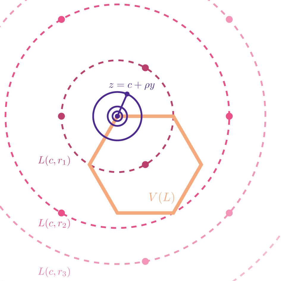


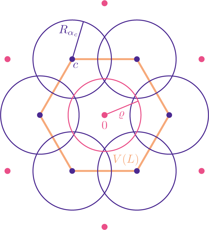

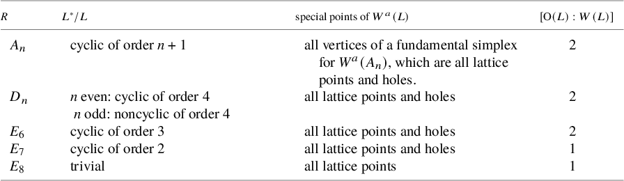
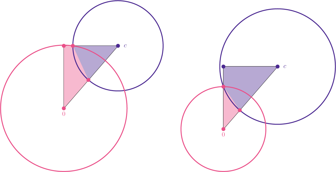
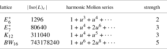


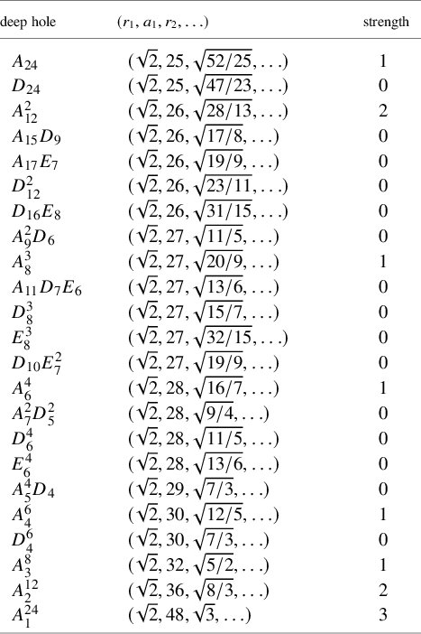


 Open access