


Impact Statement
The characterization of the effects of panel flexibility on the dynamics of separated shock–turbulent boundary layer interactions is important in high-speed flight and propulsion applications, as vibrational modes of increasingly lighter structures can couple with the low-frequency flow motions of the shock system and separation bubble. The proposed use of wall-modelled large-eddy simulation (WMLES) in a loosely coupled partitioned fluid–structure interaction simulation method results in significant savings in computational cost while maintaining physical fidelity of critical flow features such as separation and reattachment, which cannot be properly captured by lower-fidelity flow simulation methods. The reduced cost of WMLES, compared with wall-resolved LES, allows sufficiently long integration times needed to capture the low-frequency motions of interest of the flow and structure. Considering structural damping in the solid mechanics solver results in better accuracy than prior simulation efforts. By complementing experimental measurements, our numerical results indicate that the separation bubble characteristics (size and dynamics) are significantly affected by panel deformation, and can be rather sensitive to small variations in the incoming boundary layer and shock-generating method.
1. Introduction
Interactions between shock waves and turbulent boundary layers (STBLIs) are critical to the design of supersonic and hypersonic flying vehicles. Researched for decades (Reference DollingDolling, 2001), most STBLI studies have focused on interactions with boundary layers developed over rigid walls (Reference Délery and DussaugeDélery & Dussauge, 2009). The fluid–structural coupling of STBLIs has not been studied nearly as extensively despite its relevance in internal (e.g. scramjet engines) and external (e.g. aerodynamic control surfaces) flows over lightweight, thin panels (Reference McNamara and FriedmannMcNamara & Friedmann, 2011). Of particular concern is the potential coupling of vibrational modes of the panel (e.g. engine walls, control surfaces) with the characteristic low-frequency motions of the shock system and separated flow region that arise for sufficiently strong interactions (Reference Clemens and NarayanaswamyClemens & Narayanaswamy, 2014), which can lead to flow-induced cyclic loading, structural fatigue and failure. Wall deformation can, in turn, alter the flow characteristics of the STBLI, including the shock system, turbulence amplification, boundary layer development and separation.
Turbulent flows over elastic panels without the influence of incident shock have also been the subject of recent investigations. Reference Ostoich, Bodony and GeubelleOstoich, Bodony, and Geubelle (2013) numerically studied the interaction between a thin steel panel and a compressible turbulent boundary layer with  $M_\infty = 2.25$ (similar to the experiments conducted by Reference Beberniss, Spottswood and EasonBeberniss, Spottswood, and Eason (2011)), finding that the compliant panel modified the turbulence statistics under limit-cycle oscillation. These modified turbulence statistics were found to converge back to the original rigid panel form within one integral length of the turbulent boundary layer downstream of the panel. Reference Sullivan and BodonySullivan and Bodony (2019) performed high-fidelity two-dimensional laminar unsteady simulations in conjunction with the experiments of Reference Whalen, Kennedy, Laurence, Sullivan, Bodony and BuckWhalen et al. (2019) of a $M_\infty = 6.04$ flow over a $35^{\circ }$ compression ramp with an embedded compliant panel. Several reduced-order models based on piston theory were assessed. Models using localized piston theory were found to have good agreement with the conducted high-fidelity simulations. Reference Whalen, Schöneich, Laurence, Sullivan, Bodony, Freydin and BuckWhalen et al. (2020) experimentally investigated the effect of aerothermal heating on the same flow with a compliant panel and observed enhanced static deformations and frequency shifting. Comparison with an equivalent rigid panel configuration showed evidence of panel vibration in the downstream portion of the flow field.
Recently, an increasing number of experiments have investigated the coupling of STBLIs with flexible panels. Reference Spottswood, Eason and BebernissSpottswood, Eason, and Beberniss (2012) performed oblique shock impingement experiments on a compliant panel that was fixed on all four sides. In a sequence of experiments targeting statistically quasi-two-dimensional configurations of oblique STBLIs impinging on a rectangular thin flexible panel, Reference Willems, Gulhan and EsserWillems, Gulhan, and Esser (2013) and Reference Daub, Willems and GülhanDaub, Willems, and Gülhan (2016) investigated the effects of the free-stream Mach number ( $M_{\infty }$) and the incident oblique shock angle ( $\theta$). By carefully controlling the pressure differential across the flexible panel, Reference Varigonda and NarayanaswamyVarigonda and Narayanaswamy (2019) investigated interactions resulting in concave and convex panel curvature. Reference Tripathi, Mears, Shoele and KumarTripathi, Mears, Shoele, and Kumar (2020) assessed the effects of the Reynolds number, shock impingement location and cavity pressure on the panel dynamics and separation bubble characteristics in $M_{\infty } = 2$ oblique STBLIs. Testing $M_{\infty } = 2$ oblique and $M_{\infty } = 1.4$ normal STBLI–panel coupling, Reference Gramola, Bruce and SanterGramola, Bruce, and Santer (2020) found a strong influence of the cavity pressure on the aerostructural dynamics, suggesting potential strategies of wave drag passive control through adaptive shock control bumps. Experiments of $M_{\infty } = 4$ STBLIs impinging on a thin steel panel by Reference Neet and AustinNeet and Austin (2020) observed a flattened and elongated separation region and a reduction of static pressure in the flexible configuration, relative to a rigid panel.
Several measurement challenges remain that prevent a complete characterization of these coupled interactions, especially of the near-wall flow physics, from experiments alone (Reference Riley, Perez, Bartram, Spottswood, Smarslok and BebernissRiley et al., 2019). Numerical simulations thus play a crucial role to complement experiments and provide missing fundamental insight. To predict aerodynamic forces acting on a deforming structure, simplified formulations based on piston, Van Dyke and shock-expansion theories are common for quasi-steady interactions, due to the minimal computational cost (Reference Brouwer and McNamaraBrouwer & McNamara, 2019; Reference McNamara and FriedmannMcNamara & Friedmann, 2007; Reference Sullivan and BodonySullivan & Bodony, 2019; Reference Sullivan, Bodony, Whalen and LaurenceSullivan, Bodony, Whalen, & Laurence, 2020). For higher physical fidelity, prior studies have resorted to solving the inviscid Euler flow equations (Reference VisbalVisbal, 2012) or the Navier–Stokes equations via Reynolds-averaged Navier–Stokes (RANS) approaches (Reference Gogulapati, Deshmukh, Crowell, McNamara, Vyas, Wang and EasonGogulapati et al., 2014; Reference Shahriar, Shoele and KumarShahriar, Shoele, & Kumar, 2018; Reference VisbalVisbal, 2014; Reference Yao, Zhang and LiuYao, Zhang, & Liu, 2017), detached-eddy simulations (Reference Gan and ZhaGan & Zha, 2016), large-eddy simulation (LES) (Reference Borazjani and AkbarzadehBorazjani & Akbarzadeh, 2020; Reference Pasquariello, Hickel, Adams, Hammerl, Wall, Daub and GülhanPasquariello et al., 2015) or direct numerical simulation (Reference Shinde, McNamara, Gaitonde, Barnes and VisbalShinde, McNamara, Gaitonde, Barnes & Visbal, 2018), coupled with structural solvers (Reference Schemmel, Collins, Bhushan and BhatiaSchemmel, Collins, Bhushan, & Bhatia, 2020). Although attractive from a computational cost standpoint, RANS approaches cannot accurately predict strong flow separation and associated low-frequency dynamics in STBLIs (Reference Sadagopan, Huang, Xu and YangSadagopan, Huang, Xu, & Yang, 2021). The stringent grid resolution requirements of direct numerical simulation and wall-resolved LES render these simulation methods still prohibitively expensive beyond moderate Reynolds numbers, particularly for the long integration times required to capture low-frequency motions and under interactions with spanwise inhomogeneity (brought, for example, by the panel deflection).
Wall-modelled LES (WMLES) (Reference Bose and ParkBose & Park, 2018; Reference Larsson, Kawai, Bodart and Bermejo-MorenoLarsson, Kawai, Bodart, & Bermejo-Moreno, 2016) greatly reduces the computational cost of simulating wall-bounded turbulence by modelling, instead of resolving, the inner region of the turbulent boundary layer up to approximately  $10\,\%$ of the boundary layer thickness (including the viscous, buffer and part of the logarithmic sublayers). Prior work has proven WMLES capable of capturing the flow physics of non-equilibrium, separated STBLIs over adiabatic rigid walls, enabling simulations with long integration times, critical to the analysis of low-frequency unsteadiness, and of interactions with three-dimensional effects (Reference Bermejo-Moreno, Campo, Larsson, Bodart, Helmer and EatonBermejo-Moreno et al., 2014).
The present work focuses on the numerical simulation of a  $M_{\infty } = 3$ strongly separated impinging STBLI over a rectangular flexible panel, replicating the experiments of Reference Daub, Willems and GülhanDaub et al. (2016). The main novelty regarding the numerical methodology resides in the coupling of WMLES (employing an equilibrium-based wall stress model; Reference Kawai and LarssonKawai and Larsson (2012)) and a finite-element solid mechanics solver that incorporates structural damping. The use of WMLES enables the simulation to be performed at the same Reynolds number ( $Re_{\infty }=49.4\times 10^6\ \mathrm {m}^{-1}$), spanning the full panel width and for the same duration as reported in the experiments, allowing for a more complete characterization of STBLI low-frequency motions and coupling with the flexible panel dynamics. Previous numerical studies of the same experiments were conducted by Reference Pasquariello, Hickel, Adams, Hammerl, Wall, Daub and GülhanPasquariello et al. (2015) and Reference Zope, Horner, Collins, Bhushan and BhatiaZope, Horner, Collins, Bhushan and Bhatia (2021). The former used wall-resolved LES and a finite-element method hyperelastic Saint–Venant–Kirchoff solid solver that neglected structural damping, with a cut-cell immersed boundary method treatment of the fluid–solid interface. The simulation ran for a shorter duration, remaining in a transient state. Reference Zope, Horner, Collins, Bhushan and BhatiaZope et al. (2021) utilized both dynamic hybrid RANS/LES and RANS approaches for the flow solver, also neglecting damping in the solid mechanics solver.
This paper is organized as follows. The problem set-up is introduced in § 2, followed by the description of the computational methodology in § 3. Simulation results for rigid- and flexible-wall cases, considering full-span and spanwise periodic domains, are presented in § 4. When available, simulation results are compared with experimental data and prior numerical studies. Additional quantities not present in experimental studies such as separation bubble statistics, wall pressure spectral density distribution and full-panel deflection are also discussed. The main conclusions of the study are highlighted in § 5.
2. Problem set-up
The simulations performed in this study are modelled after the experiments of Reference Daub, Willems and GülhanDaub et al. (2016). A compression wedge (of  $30^{\circ }$ angle) in a $M_{\infty } = 3$ air stream generates an oblique shock that impinges on the turbulent boundary layer developed over a plate with a rectangular elastic insert. Figure 1 shows schematically the experimental set-up and the computational domain of the present simulations, which extends $80$ mm upstream and $40$ mm downstream of the rectangular flexible panel. The leading edge of the rigid wall in the experiments (origin of the absolute $x$ coordinate direction) extends $130$ mm farther upstream from the inlet to the simulations, producing a fully turbulent boundary layer. At the reference station located at $x=210$ mm, the boundary layer thickness based on 99 % of the free-stream velocity is $\delta _0=4$ mm. The compression wedge spans the full domain width $Z_d$ and rotates around point $C$ with an angle relative to the horizontal plane, $\theta$, that varies with time before reaching a value of $17.5^{\circ }$ in about $15$ ms, as shown at the top right of figure 1. The incident oblique shock generated at the wedge front (point $A$) and the front wave of the head of the expansion wave generated at the wedge rear (point $E$) intersect the top boundary of the computational domain ( $y=100\ \text {mm}=25\delta _0$) at points $P$ and $Q$, respectively, whose streamwise location and distance vary with time as the wedge rotates, before reaching constant values. The fast initial rotation of the compression wedge drives the initial excitation of panel vibrations. Computationally, this time-dependent boundary condition is implemented using Rankine–Hugoniot and Prandtl–Meyer inviscid-theory relations to determine the flow properties. The (inviscid) impingement point, $I$, used as an origin streamwise location ( $x_I=0.328\ \text {m}$) in several figures presented in this study, corresponds to the intersection of the incident oblique shock with the nominally rigid wall calculated from inviscid theory (i.e. without accounting for the boundary layer) and excluding the curvature of the incident shock induced by the interaction with the Prandtl–Meyer expansion generated at the rear corner of the wedge.
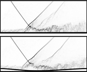
Problem set-up following experiments by Reference Daub, Willems and GülhanDaub et al. (2016) with the simulation domain highlighted in grey on the back vertical plane. Coloured contour maps are obtained from an instantaneous snapshot at  $t=15$ ms from the full-span simulation of the present study, showing the flexible panel vertical displacement, $Y_s$, the streamwise component of the wall shear stress vector, $\tau _{w,x}$ (in translucent colour), and the streamwise component of the fluid flow velocity, $u$. The latter is shown on a cropped vertical slice ( $xy$) at the centre of the spanwise domain, highlighting the incident and reflected shocks, the turbulent boundary layer and the separation bubble.

The elastic panel, made of CK 75 spring steel (see tables 1 and 2), spans  $200$ mm in the transverse direction ( $z$), and has a thickness $h=1.47$ mm. In the experiments, the flexible panel was riveted to the upstream and downstream rigid plate sections with two lines of rivets per transverse edge. In the present simulations, the elastic panel is fixed on its transverse ends to the rigid walls. The flexible panel streamwise length is $320\ \text {mm}$, corresponding to the distance between the lines of outer rivets used in the experiments. The longitudinal edges of the elastic panel, sealed with soft rubber from an underneath cavity in the experiments, are modelled by free boundary conditions in the simulations. In an attempt to minimize variations of the flow statistics in the spanwise direction, the wind tunnel sidewalls in the experiments were sufficiently far away from the tested panel. The sidewalls are thus not modelled in the present numerical study, which includes simulations that consider two configurations: one with the full span of the panel ( $Z_{d,{full}}=200\ \text {mm} = 50 \delta _0$) and another that assumes spanwise periodicity with a reduced spanwise width ( $Z_{d,{sp}}=20\ \text {mm} = 5 \delta _0$) equal to five times the incoming boundary layer thickness at the reference station (located at $x=200$ mm), denoted as $\delta _0$. Comparison of simulation results in the full-span and spanwise-periodic configurations is used to assess three-dimensional effects stemming from the flexible panel deformation. Additionally, the sensitivity to the thickness of the incoming boundary layer and to the shock strength is evaluated on the spanwise-periodic simulation configuration in § 4.
Free-stream flow variables: Mach number,  $M_{\infty }$; pressure, $p_{\infty }$; temperature, $T_{\infty }$; velocity, $u_{\infty }$. Thickness of the incoming turbulent boundary layer, $\delta _0$, at the reference location ( $x_0=200$ mm). Streamwise location of incident shock impingement over the rigid wall from inviscid theory, $x_I$, for the maximum deflection angle of the compression wedge.

Properties of the flexible panel: Young modulus,  $E_s$; Poisson ratio, $\nu _s$; density, $\rho _s$; thickness, $h$; primary natural frequency, $f_n$; mass damping coefficient, $a$. Reference time at the first peak of panel deflection, $t_0$.

3. Computational methodology
The present simulations are performed with an in-house flow–structure interaction (FSI) solver that uses a loosely coupled partitioned approach whereby the flow and solid domains are discretized with unstructured, body-fitted meshes. At the fluid–solid interface, the two meshes are non-conformal, allowing for a coarse solid mesh and fine flow mesh to exchange information via interpolation. The FSI solver consists of three specialized solvers for the fluid flow, solid mechanics and fluid mesh deformation. For the rigid wall simulations, only the flow solver is used.
The flow solver uses a finite-volume cell-centred formulation of the spatially filtered compressible Navier–Stokes (LES) equations on an unstructured hexahedral-cell mesh. Air is assumed as a calorically perfect gas with a dynamic viscosity modelled by Sutherland's law. For FSI simulations, the motion and deformation of the mesh are accounted for by an arbitrary Lagrangian Eulerian formulation of the conservation equations. Hybrid second-order numerics combine an essentially non-oscillatory scheme near shocks with a centred scheme away from shocks, distinguished by a sensor based on local dilatation, enstrophy and sound speed. To reduce the grid resolution requirements, the flow solver uses the subgrid-scale model of Reference VremanVreman (2004) and the equilibrium wall-stress wall model of Reference Kawai and LarssonKawai and Larsson (2012), with a mixing-length model for the turbulent eddy viscosity.
At each wall face, the simplified equilibrium wall-model ordinary differential equations are solved on a separate one-dimensional grid extending up to a wall-model exchange height  $h_{{wm}}$ from the wall. The wall model applies the instantaneous velocity, pressure and temperature from the LES grid at the exchange height as the top boundary condition, and adiabatic, no-slip boundary condition at the wall. The wall shear stress, $\tau _w$, calculated by solving the wall-model equations, is applied as the wall boundary condition to the LES grid. At the inlet, synthetic turbulence is generated using a digital filtering technique based on Reference Klein, Sadiki and JanickaKlein, Sadiki, and Janicka (2003), with the extensions proposed by Reference Xie and CastroXie and Castro (2008) and Reference Touber and SandhamTouber and Sandham (2009).
The geometrically nonlinear solid solver uses the finite-element method with  $27$-node hexahedral isoparametric elements, with a linear isotropic material model used to relate stress and strain. The governing equations of motion for the solid solver are $[M] \ddot {\boldsymbol {u}} + [C] \dot {\boldsymbol {u}} + [K] \boldsymbol {u} + \boldsymbol {f}_{{int}} = \boldsymbol {f}_{{ext}}$, where $\boldsymbol {u}$ is the local displacement vector of the solid mesh nodes relative to the previous deformed state. The mass matrix $[M]$ is diagonalized by using the lumped mass approximation, which allows for trivial inversion. To account for geometric nonlinearities, the stiffness matrix $[K]$, external force vector $\boldsymbol {f}_{{ext}}$ and internal force vector $\boldsymbol {f}_{{int}}$ are updated at the same frequency as the solid and flow mesh are deformed in the FSI solver. The internal force vector $\boldsymbol {f}_{{int}}$ is updated by taking the stiffness force $[K] \boldsymbol {u}$ just prior to updating the mesh deformation at each time step and adding it to the existing internal force. This allows for the accounting of geometric nonlinearities such as an increase in panel stiffness with increased deflection. The external force $\boldsymbol {f}_{{ext}}$ is updated using a pressure field interpolated onto the solid mesh from the flow domain. The damping matrix $[C]$ is assumed linearly proportional to the mass matrix $[M]$ by means of the mass damping coefficient, $a$, which is inferred using a weakly dampened oscillator analogy by fitting the experimentally measured time signal of vertical displacement at a probe near the panel centre obtained from Reference Daub, Willems and GülhanDaub et al. (2016) as $Y_s(t)\approx A \, {\rm e}^{-at/2} \cos (2 {\rm \pi}f_n t + \phi ) + B$, obtaining the constants $a$,
$a$,  $f_n$, $A$ and $B$. Since the damping coefficient is inferred from the panel response of a STBLI FSI experiment, it accounts not only for the structural damping of the panel but also, in part, for the damping introduced by the fluid flow in the wind tunnel and the cavity underneath the panel (e.g. by acoustic radiation). Despite these uncertainties in the determination of the structural damping coefficient, it is shown in § 4 that simulations that incorporate damping significantly improve the accuracy of the predictions. Along the transverse (upstream and downstream) edges of the panel, fixed–fixed (i.e. clamped–clamped) boundary conditions are employed. The static pressure beneath the panel is set to the free-stream pressure, as approximately maintained experimentally in the cavity below the panel. The longitudinal edges (located on $xy$ planes) of the panel remain free to move (i.e. not clamped). In the experiments, a soft rubber foam (not modelled) was used along the edges to seal the cavity. Time integration is performed using the same four-stage explicit Runge–Kutta method used in the flow solver.
The mesh deformation solver uses a face-based spring-system analogy by which each face of the flow mesh is treated as a spring connecting the centroids of the adjacent mesh cells sharing that face. The stiffness of each spring is inversely proportional to the square of the spring (inter-cell) distance. Dirichlet conditions are prescribed along the part of the bottom boundary of the flow mesh corresponding to the interpolated nodal positions of the deformed solid mesh. On the side boundaries (planes normal to the spanwise coordinate direction), the mesh deformation is constrained to the vertical ( $y$) direction. The mesh deformation is restricted to a region of influence above the flexible panel up to $y\leq 4 \delta _0$ for improved computational performance. The resulting linear system of equations is equivalent to a static finite-element assembly of three-dimensional trusses (Reference RaoRao, 2005).
The flow domain is discretized using hexahedral-cell, body-fitted meshes that deform with the flexible panel. Near-wall grid spacing follows Reference Larsson, Kawai, Bodart and Bermejo-MorenoLarsson et al. (2016). The first near-wall layer below the wall-model exchange location, chosen as  $10\,\%$ of the reference boundary layer thickness ( $y< h_{{wm}}=0.1\delta _0$), includes four cells with uniform grid spacing (i.e. $\Delta y=0.25 h_{{wm}}$), intended to reduce numerical errors from the LES transferred to the wall model (Reference Kawai and LarssonKawai & Larsson, 2012) and avoid the log-layer mismatch. Above the exchange location ( $h_{{wm}}< y<\delta _0$), the wall-normal spacing increases away from the wall following a hyperbolic tangent law up to $\Delta y = 0.05\delta _0$ at $y=\delta _0$, then remains uniform up to $y=4\delta _0$, and stretches again up to the top boundary ( $4\delta _0< y<25\delta _0$) with another hyperbolic tangent law. Uniform mesh spacing is used in the streamwise and spanwise directions, with $\Delta x \approx 0.08 \delta _0$ and $\Delta z = 0.05 \delta _0$, respectively. Grid convergence was assessed in our prior simulation study and is not repeated here (Reference Hoy and Bermejo-MorenoHoy & Bermejo-Moreno, 2021). The resulting number of cells in the flow solver mesh corresponds to approximately $20$ and $200$ million for the spanwise-periodic and full-span domains, respectively. The solid domain is discretized with $64$ cells (27-node isoparametric elements) in the streamwise direction, one cell across the panel thickness and $2$ (spanwise-periodic) or $20$ (full-span) cells in the spanwise direction. This results in a modest number of $128$ and $1280$ finite elements for the reduced and full-span simulations, respectively. Time integration employs a four-stage explicit Runge–Kutta method with a constant time step $\Delta t=10^{-7}\ \text {s}$, which is below the Courant–Friedrichs–Lewy condition for the flow solver, and within the stability limits of the solid solver.
At the fluid–solid interface, the flow and solid meshes are non-conforming. The flow mesh faces are much smaller than the solid mesh faces, due to the finer grid resolution required to capture the near-wall flow physics, compared with the structural deformation. The flow wall pressure field is spatially mean-filtered onto the coarser solid mesh. The resulting pressure imposed on each solid face is the area-weighted sum of the wall pressure acting on flow faces in contact with that solid face. The wall displacement field is interpolated onto the flow mesh using the finite-element shape functions of the solid solver: each point of the flow mesh in contact with the solid domain is matched to a quadrilateral solid face, its finite element natural coordinates are substituted back into the shape functions of that solid face.
4. Results
We first assess the three-dimensionality of the interaction by conducting a FSI simulation that includes the full span of the experimental panel ( $Z_d=200\ \text {mm}=50\delta _0$), comparing results with a prior spanwise-periodic simulation over a reduced span ( $Z_d=20 \text {mm}=5\delta _0$) (Reference Hoy and Bermejo-MorenoHoy & Bermejo-Moreno, 2021) and available experimental measurements (Reference Daub, Willems and GülhanDaub et al., 2016). The sensitivity of the STBLI strength to variations of the incoming boundary layer thickness and the compression wedge extent is then evaluated for spanwise-periodic simulations with the reduced span over a rigid wall. Finally, we analyse the impact of panel flexibility on the flow physics, comparing simulation results between rigid and flexible wall cases with a stronger interaction than previously reported (Reference Hoy and Bermejo-MorenoHoy & Bermejo-Moreno, 2021). When appropriate, we non-dimensionalize the time, streamwise, wall-normal and spanwise coordinates as $t' = f_n (t - t_0)$, $x' = (x - x_I) / \delta _0$, $y' = y / \delta _0$ and $z' = (z - Z_d/2) / \delta _0$, respectively, where $f_n$ is the panel first natural frequency, $t=0$ is the start time of the compression wedge rotation, $t_0$ is the reference time at the first peak of panel deflection, $x_I$ is the inviscid shock impingement location for the maximum deflection angle of the compression wedge ( $\theta _{{max}}=17.5^{\circ }$), $Z_d$ is the spanwise domain width and $\delta _0$ is the reference boundary layer thickness (see tables 1 and 2).
Based on the observed temporal evolution of the panel spatially averaged kinetic energy and the flow separation bubble dynamics (see figure 2), we identify three phases of the present FSI termed transient, transition and long-term phases. The transient phase corresponds to the rotation of the wedge from zero deflection until reaching the set point of  $17.5^{\circ }$. This transient phase is characterized by the largest panel deflection (reached halfway during the wedge rotation and followed by a slower decay) and the formation of the shock system and the flow separation bubble, whose volume rapidly increases after an initial lag of approximately $1$ ms, reaching a statistically stationary value by the end of the transient phase. In the transition phase, the kinetic energy of the flexible panel slowly decreases over approximately eight cycles of primary natural vibration before reaching a statistically stationary value that defines the long-term phase. For the strongly separated STBLI considered in this study and its associated low-frequency flow motions, the flexible panel never reaches a fully static state. Instead, in the long-term phase, the panel reaches a limit-cycle oscillation state where the rate of energy lost from damping is balanced by the rate of energy added from the pressure fluctuations and low-frequency motions from the STBLI. The magnitude of these vibrations scales roughly with the inverse of the damping ratio $\zeta$. These panel oscillations remain coupled with the STBLI flow dynamics.
Temporal evolution of dimensionless specific panel kinetic energy  $\overline {u_s^2} / (f_n \delta _0)^2$ (shown in blue with a logarithmic scale on the left-hand vertical axis), separation bubble volume $V_b / (Z_d \delta _0^2)$ (shown in red with a linear scale on the right-hand vertical axis) and wedge angle $\theta$ (shown in green with a linear scale on the right-hand vertical axis).

4.1 Three-dimensionality of panel displacement, skin friction and wall pressure
Figure 3(a) shows contours of the vertical deflection of the flexible panel along the midspan plane ( $z=0$ mm) as a function of time and streamwise direction, obtained from the full-span FSI simulation. Nonlinearity and asymmetry dominate the panel deflection, characterized by an initial transient period ( $t'<3$). Starting from an equilibrium condition with zero panel deflection at $t=0$, when the pressure on both sides of the panel is the same, the increased pressure force produced by the impinging oblique shock generated by the rotating compression wedge deflects the flexible panel. After the first peak of panel deflection is reached at $t=t_0$, damped oscillations occur about a mean deflection state. A quantitative comparison of the panel deflection as a function of time is presented in figure 3(b) for three probe locations where experimental measurements were reported by Reference Daub, Willems and GülhanDaub et al. (2016). These probes were placed along the panel centreline ( $z = Z_d/2$) at streamwise locations $x = 295$, $375$ and $445$ mm, denoted front, centre and rear, respectively. The vertical dashed lines in figure 3(a) correspond to the three probe locations. The time signals of panel deflection at the three probes shown in figure 3(b) compare results from the full-span simulation, spanwise-periodic simulation with a reduced span and experiments.
(a) Contours of vertical panel displacement,  $Y_s / \delta _0$, along the midspan plane as a function the streamwise coordinate and time, obtained from the full-span simulation. Grey colours indicate positive vertical deflection. (b) Time signals of panel displacement measured at the front (red), centre (blue) and rear (green) probe locations marked by vertical dashed lines in (a), comparing results from full-span simulations (solid), previous spanwise-periodic reduced-span simulations (dashed) by Reference Hoy and Bermejo-MorenoHoy and Bermejo-Moreno (2021) and experiments (dotted) by Reference Daub, Willems and GülhanDaub et al. (2016).

Full-span simulations predict the experimental deflection measurements with reasonable accuracy, especially for the centre probe. The largest differences are observed for the front and rear probes near the first two peaks of deflection, which are over- and under-predicted, respectively. After the transient, signals for the three probes recover dampened oscillations around a mean deflection curve in close agreement with experiments, including the amplitudes and frequencies of oscillation. Contributing factors to the observed differences from experiments include: (1) the large sensitivity of panel displacement to the exact probe streamwise location, observed in figure 3(a); (2) the modelling of the transverse rows of rivets used in the experiments with a simplified fixed–fixed boundary condition in the simulations; and (3) neglecting, in the simulations, the foam sealing on the streamwise edges of the flexible panel used experimentally to prevent leakage into the underneath cavity, which may increase the stiffness along the edges (Reference Willems, Gulhan and EsserWillems et al., 2013). The use of a mass proportional damping model provides a reasonable approximation of primary modal damping of the panel (compare, for example, with prior FSI simulations without damping by Reference Pasquariello, Hickel, Adams, Hammerl, Wall, Daub and GülhanPasquariello et al. (2015)), but with limitations. Damping effects caused by the foam sealing along the sides are not modelled. Also, with mass proportional damping, higher-frequency vibrations have smaller damping ratios than the primary frequency, so high-frequency content takes longer to damp out.
We assess in figure 4 the three-dimensionality of the flow through contour plots of the panel deflection, skin friction coefficient and wall pressure, mapped on the flexible panel and projected onto the horizontal ( $xz$) plane, time-averaged after the initial transient. Three-dimensional effects are most noticeable in the panel deflection (figure 4a) near the longitudinal edges ( $|z'|>15$), where the deflection exceeds that of the panel centreline, especially for streamwise locations of maximum wall pressure ( $0\lesssim x' \lesssim 20$). The foam sealing (not modelled in the present simulations) used in the experiments along the longitudinal edges (Reference Daub, Willems and GülhanDaub et al., 2016) may add a slight stiffness along the edges, reducing the deflection difference between the centreline and the edges of the panel. Consistent with our fixed–fixed (along transverse edges) panel model, detailed static finite-element simulations performed by Reference Willems, Gulhan and EsserWillems et al. (2013), which accounted for panel riveting, also found the panel deflection to be larger along the edges of the panel. Contours of the time-averaged skin friction coefficient (figure 4b) show a predominantly two-dimensional character, except very near the longitudinal edges ( $|z'|>20$) downstream of the inviscid impingement location ( $x'>0$), which may be attributed to the symmetry (slip-wall) boundary conditions imposed by the flow solver on the side boundaries of the computational domain for this full-span simulation. Downstream of the boundary layer reattachment ( $15\lesssim x' \lesssim 40$), the time-averaged skin friction exhibits streamwise streaks leading to ragged spanwise contours. These are attributed to larger-scale turbulent flow structures produced by the shear layer resulting from the STBLI (see figures 1 and 6b) and Görtler-like vortices, previously found in wall-resolved LES by Reference Pasquariello, Hickel and AdamsPasquariello, Hickel, and Adams (2017) of the rigid-wall STBLI, with a spanwise wavelength of approximately $2\delta _0$, requiring much longer averaging time periods to homogenize. Lastly, the time-averaged wall pressure contours shown in figure 4(c) exhibit minimal three-dimensionality. In conclusion, the presently studied interaction can be approximated as statistically two-dimensional, enabling the use of spanwise-periodic simulations, which is the focus of the remaining analysis.
(a) Normalized panel displacement,  $Y_s/\delta _0$, (b) skin friction coefficient, $C_f \times 10^3$, and (c) normalized wall pressure, $p_w/p_{\infty }$, time-averaged ( $t \in [20,60]$ ms) on the streamwise–spanwise ( $xz$) plane, for the full-span FSI simulation.

4.2 Sensitivity of the STBLI to wedge length and incoming boundary layer thickness
Two main sources of uncertainty when comparing the present simulations with experiments stem from viscous effects of the flow around the compression wedge and the development of the incoming boundary layer. The compression wedge that generates the oblique shock impinging on the panel is not included in the computational domain, but its effect is modelled through the top boundary of the flow computational domain, where time-varying Rankine–Hugoniot and Prandtl–Meyer inviscid flow conditions are prescribed, following Reference Pasquariello, Hickel and AdamsPasquariello et al. (2017). While effective at reducing the computational cost, such top boundary condition neglects the wedge boundary layers and wake, which can alter the Prandtl–Meyer expansion generated at the rear corner of the wedge and its interaction with the oblique shock, thus affecting the strength of the STBLI on the panel (see figure 1). A second source of uncertainty arises from an incomplete characterization of the incoming boundary layer in the experiments, which relied on Pitot-rake and global turbulent intensity (longitudinal and transverse) measurements at one location ( $x=150$ mm) upstream of the STBLI. The strength of the interaction and, in turn, the extent of flow separation depend on the incoming boundary layer thickness (Reference Zhou, Zhao and ZhaoZhou, Zhao, & Zhao, 2019).
We assess in figure 5 the effects of these uncertainties on the wall-pressure profiles characterizing the STBLI from two parametric studies conducted on spanwise-periodic rigid-wall simulations by: (1) extending the wedge length by a factor  $\xi$ (in $2~\text {mm}$ increments), for the same wedge angle of $30^{\circ }$, which delays the interaction of the expansion fan and the shock; and (2) modifying the incoming boundary layer thickness by a factor $\eta$ relative to the reference value inferred experimentally of $\delta _0=4$ mm. A subset of the simulation results is presented in figure 5, for clarity. As seen in figure 5(a), wedge length extensions strengthen the STBLI, which is initiated farther upstream and reaches a larger pressure peak for increasing $\xi$, while preserving a similar pressure profile shape. In contrast, a thicker incoming boundary layer alters the shape of the pressure profile by also bringing the initial pressure rise (corresponding to the separation shock) farther upstream while decreasing the maximum wall pressure reached throughout the STBLI (figure 5b). Comparison with experimental wall-pressure profiles provided the best agreement for a $6$ mm wedge extension ( $\xi =1.069$) and an incoming boundary layer $20\,\%$ thicker than the $4$ mm reference value ( $\eta =1.2$). These values are used in the spanwise-periodic, rigid- and flexible-wall simulations presented in the remaining sections to evaluate the effect of panel flexibility on the STBLI.
Sensitivity of streamwise profiles of time- and spanwise-averaged wall pressure over a rigid panel to variations in (a) wedge length ( $\xi$) for an incoming boundary layer thickness with $\eta =1.2$ and (b) incoming boundary layer thickness ( $\eta$) for a wedge extension with $\xi =1.069$. Symbols represent experimental measurements by Reference Daub, Willems and GülhanDaub et al. (2016).

4.3 Effects of panel flexibility on wall pressure, skin friction and separation bubble characteristics
A qualitative comparison of rigid and flexible mean streamwise velocity contours and instantaneous density gradient magnitude along the midspan plane ( $z = Z_d/2$) and above the panel insert ( $210\ \text {mm} \leq x \leq 530$ mm) is shown in figure 6 (time-series animations comprising the total integration time of the simulations are provided as supplementary movies available at https://doi.org/10.1017/flo.2022.28). The turbulent boundary layer separates and reattaches due to the interaction with the shock system, significantly thickening downstream.
Flexible (bottom) and rigid (top) panel comparison of (a) mean streamwise velocity  $\bar {u}$ and (b) numerical schlieren $|\nabla \rho |$, above the panel ( $210 \leq x \leq 530$ mm), along the midspan plane ( $z=0$ mm), time-averaged ( $t \in [20,60]$ ms) for rigid- and flexible-wall simulations, zooming into the STBLI region. White contour lines on the mean velocity plots mark the time-averaged region of flow reversal. An animation for the full integration time of the simulation is provided as supplementary movies.

The temporal evolution of wall pressure is significantly affected by panel flexibility, as shown in figure 7. Compared with the rigid-wall case, for which the pressure remains uniform upstream of the separation shock, the deformation of the flexible panel induces a clear drop of wall pressure upstream of the shock impingement, consistent with the supersonic flow over the diverging geometry that results from the panel deflection. This upstream drop in pressure over the panel prior to flow separation is accurately estimated by local piston theory as described in Reference Sullivan and BodonySullivan and Bodony (2019). The wall pressure is modulated by the panel vibrational frequencies, which vary throughout the panel streamwise extent and can be mapped to the panel displacement frequencies seen in figure 9(a) (compare the regions near the start and end of the panel, for example, with higher and lower vibrational frequencies, respectively, and the corresponding wall-pressure modulation). The pressure rise corresponding to the separation shock is brought farther upstream in the flexible case.
Contours of spanwise-averaged wall pressure  $p_w / p_{\infty }$ as a function of streamwise coordinate and time for rigid (a) and flexible (b) panel simulations. Vertical dashed lines mark the extent of the flexible panel.

We present in figure 8(a,b) streamwise profiles of the wall pressure,  $p_w$, and the friction coefficient, $C_f$, averaged in the spanwise $z$ direction and in time for $t \in [20,60]$ ms. Compared with the rigid-wall case, the wall pressure decreases over the flexible panel upstream of the shock impingement, as observed in figure 7. The pressure drop is accompanied by a decrease in the skin friction coefficient, leading to the boundary layer separating about $3\delta _0$ farther upstream in the flexible panel case ( $x'\approx -9.4$) than in the rigid case ( $x'\approx -6.4$). The peak wall pressure of the rigid STBLI is greater than for the flexible case. The pressure drop over the panel prior to flow separation and the reduction of peak wall pressure compared with the rigid case are also seen in numerical simulations by Reference Zope, Horner, Collins, Bhushan and BhatiaZope et al. (2021) and Reference Pasquariello, Hickel, Adams, Hammerl, Wall, Daub and GülhanPasquariello et al. (2015), and experiments by Reference Gramola, Bruce and SanterGramola et al. (2020) and Reference Varigonda and NarayanaswamyVarigonda and Narayanaswamy (2019). For the flexible panel, the wall pressure peaks farther downstream and rises (induced by the separation shock) farther upstream than in the rigid-wall configuration. To better understand fluctuations that are not directly stemming from high frequencies in the turbulent boundary layer, a low-pass filter (with a cut-off frequency $f = u_\infty / L_{{sep}}$) is applied to each of the time signals of wall pressure and skin friction followed by a calculation of standard deviation at each probe location (as shown in figure 8c,d). This follows the approach taken by Reference Pasquariello, Hickel and AdamsPasquariello et al. (2017) with an identical incoming turbulent flow over a rigid wall and a larger wedge deflection angle $\theta _{{max}} = 19.6^{\circ }$. Similar to that case, the first peak of wall-pressure fluctuations corresponds to pitching low-frequency motions from flow separation. The second peak occurs from reattachment of the shear layer. The first peak of fluctuations shows the flexible panel experiencing flow separation farther upstream and with a lower overall magnitude of fluctuation in relation to the rigid panel (when low-pass-filtered). The second peak is lower and occurs farther downstream for the flexible panel, indicating a longer distance until the flow reattaches itself.
Time- and spanwise-averaged streamwise profiles of (a) wall pressure  $p_w$ and (b) skin friction coefficient $C_f$. Zoomed-in flexible- and rigid-panel comparison of band-limited ( $St_{{sep}} = f L_{{sep}} / u_\infty < 1$) root mean square of (c) wall-pressure $p_w^\prime$ fluctuations and (d) streamwise skin friction $C_f^\prime$ fluctuations. Solid red line, rigid-panel WMLES; solid blue line, flexible-panel WMLES FSI; dashed red line with symbols, rigid experimental data (Reference Daub, Willems and GülhanDaub et al., 2016); dashed blue line, wall-resolved LES averaged over one oscillation period in the transient phase (Reference Pasquariello, Hickel, Adams, Hammerl, Wall, Daub and GülhanPasquariello et al., 2015). Black vertical dashed lines in (a,b) mark the extent of the flexible panel.

Panel flexibility also leads to a significant ( $60\,\%$) increase of the separation length (from $L_{{sep}}/\delta _0\approx 7.8$ to $12.6$ in the rigid and flexible cases, respectively), which translates into a larger plateau of the wall-pressure streamwise profile. Using lower-fidelity simulations, Reference Zope, Horner, Collins, Bhushan and BhatiaZope et al. (2021) also found an increase in separation length with panel flexibility. Recent experiments by Reference Neet and AustinNeet and Austin (2020) on the effect of panel compliance on STBLI at $M_{\infty } = 4$ also observed an increase in the separation length for comparable non-dimensional panel deflections.
Contours of power spectral density (PSD) of wall pressure for the rigid and flexible cases are superimposed in figure 9, along with the PSD of the flexible panel deflection, obtained after the transient ( $t'>3$). For the flexible panel case, the streamwise location of low-frequency motions is shifted upstream by approximately $3\delta _0$ and its extent is widened, indicating a larger amplitude of upstream–downstream motions of the separation shock. The intermediate frequencies, characteristic of the separation bubble region and flapping motions of the shear layer produced by the STBLI, are downshifted for the flexible panel case, extending farther downstream, consistent with the larger separation bubble length. The fundamental frequency of the panel is $f_n \approx 230\ \text {Hz}$, corresponding to a Strouhal number based on the incoming boundary layer thickness and the free-stream velocity of $St_n = f_n \delta _0 / U_{\infty } = 0.0017$. The PSD of flexible-panel deflection partially overlaps with the low-frequency motions of the flow. A higher vibrational frequency range is observed for the upstream region of the panel ( $x'<10$), where low-frequency flow motions dominate. Farther downstream, in the rear part of the flexible panel ( $x'>10$), a downshift of the primary natural frequency $f_n$ is observed.
Superposition of PSDs of wall pressure for rigid (red) and flexible (blue) walls, and of flexible panel displacement (greyscale) as a function of the streamwise location, showing the extent corresponding to the length of the flexible panel. Normalized colourbars use an arbitrary scale (the same for rigid- and flexible-wall cases).

The contribution of high-, medium- and low-frequency bands to the wall-pressure PSDs of rigid and flexible cases is compared in figures 10(a), 10(b) and 10(c), respectively. These frequency bands approximately correspond to the low-frequency motions of the STBLI ( $St<0.05$), the flapping motions of the shear layer ( $St\in [0.05,0.5]$) and the characteristic motions of the turbulent boundary layer ( $St>0.5$). Upstream of the STBLI, the high-frequency band is dominant, accounting for over $80\,\%$ of the total power. An abrupt increase in the power contribution of the low-frequency band occurs at the onset of the separation shock, accounting for approximately $70\,\%$ of power at the peak for both rigid and flexible cases. Low-frequency motions dominate over a wider streamwise region for the flexible case. The larger separation length in the flexible case translates into a longer streamwise distance where medium frequencies are also dominant, resulting in a slower downstream recovery towards the dominance of turbulent boundary layer frequencies than in the rigid case. Using the power contribution of the high- frequency band as a metric for turbulent boundary layer recovery, from the point of separation, the turbulent boundary layer over the flexible panel takes a streamwise distance of $61 \delta _0$ to recover 80 % of the mean turbulent boundary layer power contribution prior to separation. In comparison, the turbulent boundary layer over the rigid panel recovers in $\Delta x' \approx 47 \delta _0$. In consequence, the turbulent boundary layer recovery length is about 30 % longer for the interaction over a flexible panel. The downshift of frequencies after the separation shock for the flexible case is also seen in the PSD frequency-band distribution, where the relative contribution of the high-frequency band decreases, whereas that of the mid-frequency band increases, compared with the rigid-wall case.
Band contribution  $\eta (x)$ to the signal power of wall pressure $p_w(x)$ for (a) high-frequency band $0.5 < St < \infty$, (b) medium-frequency band $0.05 < St < 0.5$ and (c) low-frequency band $0 < St < 0.05$. (d) Comparison of rigid and flexible wall pressure PSD for the low-frequency motions (solid line) and the separation bubble (dashed line). Red line, rigid panel; blue line, flexible panel.

Figure 10(b) compares the streamwise-averaged PSD of wall pressure at the locations dominated by low-frequency motions ( $x' \in [-9.4,-8.9]$ for the rigid case and $x' \in [-12.6, -12.1]$ for the flexible case) and near the separation bubble ( $x' \in [-5.0, 10.0]$ for the rigid case and $x' \in [-7.5, 12.0]$ for the flexible case). The drastic shift of dominant frequencies between both regions is clearly seen for both rigid- and flexible-wall cases. In the separation bubble region, a notable downward shift of dominant frequencies is observed for the flexible case. In the low-frequency motion region, the overall spectral distribution is more similar between the two cases but the dominant frequency is also lower for the flexible case than for the rigid case, indicative of another downward shift of dominant frequencies.
The effect of panel flexibility on the volume and streamwise centroid position of the separated flow region induced by the STBLI is quantified in figure 11(a), which compares the joint probability density functions (PDFs) between the rigid and flexible cases, time-averaged ( $t\in [20, 60]$ ms). The separation bubble volume $V_b$ is non-dimensionalized by the reference boundary layer thickness $\delta _0$ and the spanwise domain width $Z_d$ such that $V_b^* = V_b / (\delta _0^2 Z_d)$. The marginal PDFs show predominantly Gaussian shapes with a mean non-dimensional bubble volume $\mu _s = (9.4, 4.3)$ and a standard deviation $\sigma _s = (0.75, 0.37)$ for the flexible and rigid cases, respectively, with a similar ratio $\mu _s / \sigma _s \approx 12$ found in both cases. Panel flexibility induces a small negative correlation between the separation bubble volume and its streamwise centroid position, by which the bubble tends to be largest when its centroid is at its most upstream locations. This correlation is absent in the rigid-wall case. The spectral distribution of the separation bubble volume exhibits a downward shift of dominant frequencies with panel flexibility, as also noticed in the PSD of wall pressure in the separation bubble region (figure 10d). This downward shift is partially accounted for when scaling the frequencies by the separation lengths (instead of the reference boundary layer thickness) for each panel configuration, as shown in figure 11(b).
(a) Joint and marginal probability distribution (shown with contour lines) of separation bubble volume and separation bubble  $x$-centroid, after the transient, $t' > 3$, with Gaussian distribution fits shown in the marginal PDFs. Markers in the joint PDF correspond to sampled snapshots every 100 time steps. (b) Premultiplied and normalized PSD of separation bubble volume scaled by the Strouhal number based on the separation length ( $St_{{sep}} = f L_{{sep}} / u_{\infty }$). The flexible-panel results are shown in blue and the rigid-panel results are shown in red.

As a surrogate for the shape of the separation bubble, figure 12(a) shows the projection on a vertical plane of the time- and spanwise-averaged probability distribution of instantaneous flow reversal ( $u<0$) after the transient period ( $t' > 3$), comparing the rigid and flexible cases. The mean wall position $Y_s(x)$ is shown with dashed lines and the separation bubble centroids $(\bar {x}, \bar {y})$ are marked with crosses, for reference. The spatially integrated probability of instantaneous flow separation for the flexible case is significantly larger than for the rigid case (proportional to the mean separation bubble volumes). Figure 12(b) compares geometrical differences between the two flow separation regions not related to wall curvature and increased flow separation. In both cases, the region of flow reversal remains mainly confined to the boundary layer, and is biased towards the region between the separation bubble centroid and the shock impingement point at the wall. The flow reversal regions are predominantly triangular, with panel flexibility resulting in a slight flattening, shortening the relative wall-normal height, when normalized by the separation length.
(a) Time- and spanwise-averaged probability distributions of flow reversal for the rigid (top) and flexible (bottom) panel cases for  $t' > 3$. The average wall deflection, $Y_s(x)$, is shown by the dashed line, and the separation bubble centroids are marked with crosses. (b) Comparison of separation bubble shapes for rigid (red) and flexible (blue) cases by superimposing contour lines of the probability distributions of flow reversal shown in (a) in coordinates normalized by the separation length, $L_{sep}$, and relative to the mean separation bubble $x$-centroid, $\bar {x}$, and to the mean wall vertical location, $Y_s(x)$.

4.4 Assessment of lower-fidelity modelling simplifications: inviscid flow, one-way coupling and local piston theory
To elucidate the effect of several modelling simplifications commonly used in lower-fidelity methodologies, we show results from additional spanwise-periodic simulations with: (1) a two-way coupled FSI simulation using the inviscid flow assumption (i.e. with a slip wall boundary condition) and uniform inflow (set to the free-stream conditions); (2) a one-way coupled simulation that considers the wall pressure time history from a precursor rigid flat-wall simulation and solves for the panel deformation using the solid mechanics solver with the time-varying wall pressure imposed as the top boundary condition; and (3) a one-way coupled simulation that applies local piston theory (as described in Reference Sullivan and BodonySullivan and Bodony (2019)) to obtain a correction to the wall pressure field, which is then used as a new time-varying boundary condition to the solid solver to provide the panel displacement field over time. The results of these simulations are compared with those obtained with the proposed fully coupled WMLES FSI methodology.
Figure 13 shows the spatiotemporal contours of spanwise-averaged wall pressure for the original spanwise-periodic fully coupled FSI simulation and the three simplified modelling approaches (zooming into a time period of interest, relative to the longer time span shown in figure 7). As expected, the inviscid flow assumption results in large discrepancies of this quantity, both in the range of values attained (the maximum wall pressure is much higher than in the viscous cases) as well as in the upstream extent of the STBLI. The vibrations of the flexible panel are still felt by the flow through wall-pressure oscillations, strictly due to curvature effects, as noticed particularly upstream of the shock impingement location. The piston-theory correction recovers qualitative features of the FSI, naturally absent in the rigid WMLES, but largely over-predicts the maximum pressure and cycles after the transient, relative to the fully coupled WMLES FSI. The patterns of wall-pressure oscillation downstream of the interaction are also captured with lower accuracy.
(a–d) Streamwise wall pressure  $p_w$ comparison of fully coupled WMLES FSI with rigid WMLES, piston-theory correction of rigid WMLES and fully coupled inviscid FSI.

Both the two-way coupled FSI simulations with an inviscid flow approximation and one-way coupled simulation with piston-theory correction to the rigid WMLES provide qualitatively reasonable estimates of the panel displacement in the transient phase, as shown in figure 14. However, significant quantitative differences can be observed when comparing front, centre and rear probe measurements over time (see figure 15). Nonetheless, local piston-theory correction provides a significant improvement in accuracy over the one-way coupled simulation that imposes the pressure history from a rigid WMLES.
Vertical panel displacement  $Y_s$ as a function of streamwise location and time, comparing fully coupled FSI with WMLES (a) and inviscid flow assumption (b), one-way coupling with pressure from a precursor rigid WMLES (c) and one-way coupling FSI with piston-theory correction of the rigid WMLES pressure (d).

Time signals of vertical panel displacement at front (red), centre (blue) and rear (green) probe locations of streamwise location and time, comparing fully coupled FSI using WMLES (a); fully coupled FSI using an inviscid flow assumption (b); one-way coupling with pressure from a precursor rigid WMLES (c); one-way coupling FSI with piston-theory correction of the rigid WMLES pressure (d). Solid lines correspond to the simulation results and dotted lines correspond to the experiments.

The time-averaged results from the long-term phase of interaction are shown in figure 16. The one-way coupling simulation with localized shock piston theory correction model using Lighthill's coefficients (described in Reference Sullivan and BodonySullivan and Bodony (2019)) accurately predicts the flow pressure drop above the flexible panel upstream of the flow separation. Downstream of the STBLI, the pressure shift in the downstream direction (resulting from panel deformation) is also predicted with reasonable accuracy. There are, however, two notable features that are not accurately captured by the piston-theory correction. The first is that the peak wall pressure is actually lower for the flexible panel and not higher than the rigid-panel configuration. The second feature is that the location of flow separation for the flexible panel is moved farther upstream. This simple first-order correction is quite effective but could be improved upon in future studies with additional models to account for changes in the STBLI. The two-way coupled FSI simulation with an inviscid flow solver also predicts the pressure drop above the flexible panel prior to flow separation with reasonable accuracy. Unsurprisingly, the peak pressure is over-predicted as viscous effects are neglected, and the flow does not experience separation, responsible for further smoothing out the pressure profile. Downstream of the oblique shock intersection, the inviscid model provides a reasonably accurate prediction of the wall pressure relaxation stemming from the Prandtl–Meyer expansion, but being pushed farther downstream due to the panel curvature causing larger compression effects. As a consequence of the pressure load being shifted downstream under the inviscid flow assumption, the resulting shape of the time-averaged panel vertical deflection streamwise profile is also largely biased towards downstream locations, resulting in a steeper recovery towards the end of the flexible panel that produces the overcompression seen in the pressure profile. Piston-theory correction improves the prediction, while still overestimating the peak pressure and exhibiting a smaller separation bubble (manifested by the steeper rise of pressure near the inflection point), compared with the fully coupled WMLES LES solution.
Comparison of time- and spanwise-averaged (a) pressure  $p_w$ and (b) panel deflection $Y_s$ along the streamwise ( $x$) direction using: two-way coupled WMLES FSI (solid blue); one-way coupled simulation with rigid-wall WMLES pressure time history (solid red); one-way coupling simulation with localized piston-theory correction (dotted green); two-way coupled FSI with inviscid flow assumption (dashed black).

From these observations, as the amount of flow separation increases for the STBLI, models based on piston-theory corrections may struggle to make accurate predictions in the separation region of the flow. As such, additional corrections are needed to estimate the increase in flow separation and drop in the peak mean wall pressure.
5. Conclusions
In this study, we have characterized the effects of panel flexibility on a STBLI at Mach 3, comparing rigid- and flexible-wall cases. The investigation is conducted by performing high-fidelity numerical simulations that replicate the conditions tested in previous experiments by Reference Daub, Willems and GülhanDaub et al. (2016). The simulations utilize a loosely coupled, partitioned FSI solver methodology consisting of a WMLES flow solver, an isoparametric high-order finite-element solid solver and a spring-system analogy mesh deformation solver. The proposed numerical methodology, incorporating an equilibrium wall model in the flow solver, significantly reduces the computational cost, enabling long integration times while maintaining physical fidelity, both necessary to study the strongly separated STBLI and its coupling with the flexible panel dynamics.
Comparisons of panel deflection with experimental measurements at three probe locations along the panel centreline indicate that the incorporation of structural damping in the solid mechanics solver significantly improves the predictions relative to prior simulation efforts. Time signals obtained from the front and rear probes are found to be especially sensitive to small variations in the streamwise location. After a transient period dictated by the initial compression wedge rotation, a quasi-stationary state is achieved in which low-amplitude panel oscillations (about a constant mean) induced by the flow (STBLI dynamics) are attained. The experimental deflection values and frequencies are reproduced with reasonable accuracy by the simulations. The effects of three-dimensionality induced by the panel deformation are assessed by conducting simulations that include the full span of the panel and comparing the results with those of a simulation with spanwise-periodic reduced domain.
The full-span simulation reveals that the three-dimensional effects are noticeable in the panel deflection, especially near the side boundaries, but are nearly negligible in the flow wall quantities (e.g. friction and pressure), rendering spanwise-periodic simulations suitable for studying this configuration.
The deflection of the flexible panel induced by the over-pressure resulting from the STBLI feeds back onto the flow. The footprint of panel vibration is clearly seen in the temporal evolution of wall pressure. However, upstream and downstream regions of the panel relative to the shock impingement point are affected differently: whereas the wall pressure in the upstream region is modulated by the natural frequency of panel vibration, the downstream region imposes lower frequencies of vibration. As a result of the flexible wall deflection, the strength and streamwise extent of the STBLI increase, producing a ( $\approx 60\,\%$) larger separation bubble compared with the rigid-panel configuration. Nonetheless, when normalizing by mean separation length, the flexible- and rigid-wall cases present similar shapes of mean flow reversal, with a slightly flatter triangular shape for the flexible case. The larger separation bubble found under panel flexibility pushes the low-frequency motions of the STBLI farther upstream and spreads them over a wider streamwise region than for the rigid-wall configuration. Despite the larger extent, the distribution of frequency content in the wall-pressure signal is similar in both flexible- and rigid-wall cases, with a slight downward spectral shift for the flexible case associated with the larger separation bubble. The panel deflection has a clear impact on the centre of pressure, pushing it farther downstream and correlating well to the centre deflection of the panel.
The observed effects of panel flexibility on the STBLI presently studied mainly focus on the non-transient phase of the simulation ( $t' > 3$) where mean quantities of the flow field remain relatively constant, but coupled low-frequency motions of the STBLI and oscillations of the flexible panel are present. Increasing the strength of the STBLI, reducing the structural damping and oscillating the compression wedge about the panel primary natural frequency $f_n$ would result in stronger limit-cycle oscillations and increased coupling between the panel and STBLI dynamics and should be addressed in future studies.
The assessment of simplified modelling approaches for this configuration reveals that local piston theory applied to the rigid WMLES pressure profile and the one-way FSI coupling deflection history derived from that rigid-wall pressure field can accurately predict wall-pressure drops from flow expansion upstream of the flow separation point, and wall-pressure increases from flow compression near the downstream edge of the panel. Such simplified modelling strategies are, however, not appropriate for predicting changes to the flow separation point and the peak wall pressure. Both one-way coupled piston theory and two-way coupled inviscid FSI solvers provide reasonable estimates of the long-term time-averaged panel deflection profiles, but slightly over-predict the maximum deflection magnitude and its streamwise location.
Supplementary movies
Supplementary movies are available at https://doi.org/10.1017/flo.2022.28. These are movies of the temporal evolution of flow quantities and panel deflection on the midspan plane.
Acknowledgements
Computational resources were provided by: an INCITE award allocation on the Theta supercomputer at Argonne Leadership Computing Facility (ALCF), Argonne National Laboratory; by an allocation of the Department of Energy's Predictive Science Academic Alliance Program (PSAAP3) on the Quartz supercomputer at Lawrence Livermore National Laboratory (LLNL); and by the Center for Advanced Research Computing at the University of Southern California.
Funding statement
This work has been partially supported by NASA grant 80NSSC18M0148, DOE grant DE-NA0003993 and NSF award 2143014.
Declaration of interest
The authors report no conflict of interest.
Author contributions
Conceptualization: I.B.-M., J.H. Funding acquisition: I.B.-M. Methodology: J.H., I.B.-M. Data curation: J.H., I.B.-M. Software: J.H., I.B.-M. Investigation: J.H., I.B.-M. Data visualization: J.H., I.B.-M. Supervision: I.B.-M. Writing manuscript: J.H., I.B.-M. All authors approved the final submitted manuscript.
Data availability statement
Simulation data are available upon reasonable request.
Ethical standards
The research meets all ethical guidelines, including adherence to the legal requirements of the study country.


 Open access