


Impact Statement
Autonomous air vehicles and underwater gliders are becoming commonplace to support civilian, research and military applications. These vehicles use lifting surfaces that often encounter off-design conditions such as stall and the performance of these vehicles depends on the response of the lifting surfaces to these situations. Under specific conditions (angle of attack, Reynolds number and airfoil shape), three-dimensional patterns of flow separation, also known as stall cells, are known to form on the surface. These stall cells may not affect the overall aerodynamic performance, but will limit the functionality of trailing-edge flaps and/or aeilerons etc. Therefore, it is very important to understand and ideally predict the situations where stall cells can form on a lifting surface. This will enable us to account for loss of performance (or control authority) at the design stage, leading to more efficient and functional autonomous vehicles.
1. Introduction
One of the earliest research efforts into stall by Reference McCullough and GaultMcCullough and Gault (1951) investigated the influence of the airfoil shape. It was found that mainly the airfoil thickness can distinguish three different types of two-dimensional stall. One of these types of stall, trailing-edge stall, later was investigated by Reference Moss and MurdinMoss and Murdin (1968) who observed three-dimensional stall behaviour. It was shown that a curved separation line with two spiral nodes near the trailing edge was present along the span. This flow structure is referred to as a stall cell. Reference Broeren and BraggBroeren and Bragg (2001) showed that trailing-edge stall, or a combination of trailing-edge and leading-edge stall, is required for stall cell formation. Stall cells tend to form at an angle of attack close to or beyond stall such as shown by Reference Yon and KatzYon and Katz (1998) and Reference Dell'Orso, Tuna and AmitayDell'Orso, Tuna, and Amitay (2016). Furthermore the Reynolds number has been indicated to be one of the criteria for stall cell formation by Reference ScheweSchewe (2001).
Stall cells require a minimum Reynolds number for formation; however, contrasting results have been found in the literature. Reference Elimelech, Arieli and IosilevskiiElimelech, Arieli, and Iosilevskii (2012) observed stall cells at Reynolds numbers of several tens of thousands, whereas others such as Reference Gregory and O'ReillyGregory and O'Reilly (1970), Reference ScheweSchewe (2001) and Reference Dell'Orso, Tuna and AmitayDell'Orso et al. (2016) report Reynolds numbers an order of magnitude larger for stall cell formation. The formation of stall cells is not well understood but has been reasoned by Reference Weihs and KatzWeihs and Katz (1983) to be due to a spanwise disturbance influencing the two shear layers of a wing with separated flow; this has been based on a Crow-like instability described by Reference CrowCrow (1970).
The flow mechanisms involved in a stall cell have been investigated by Reference Manolesos, Papadakis and VoutsinasManolesos, Papadakis, and Voutsinas (2014a, Reference Manolesos, Papadakis and Voutsinas2014b). It was shown that three typical vortical structures are involved in a stall cell: the trailing-edge vortex, the separation line vortex and the stall cell vortices. Each fully formed stall cell has two counter-rotating stall cell vortices that originate in the spiral nodes on the wing surface, rise up from the surface and then proceed to trail downstream. The flow structures involved in a stall cell are shown in figure 1. These findings are in line with earlier predictions made by Reference Yon and KatzYon and Katz (1998), who observed an upwash at the centre of the stall cell and a downwash outside of the stall cell due to the stall cell vortices trailing downstream.
Vortices (solid lines) and flow direction (dotted lines) of a stall cell.

Multiple experimental investigations into stall cells have used a wide variety of airfoils and wing aspect ratios (ARs). It has been shown by Reference Gregory, Quincey, O'Reilly and HallGregory, Quincey, O'Reilly, and Hall (1971) and Reference Winkelman and BarlowWinkelman and Barlow (1980) that it is possible to generate either half or full stall cells. Reference Winkelman and BarlowWinkelman and Barlow (1980) indicated that increasing the AR of a wing will result in more stall cells being formed along the wing span. This behaviour of stall cells has been reproduced by Reference Yon and KatzYon and Katz (1998) and Reference ScheweSchewe (2001), which indicates that the width of stall cells scales with the chord length of the wing. Although the average width of a stall cell can be approximated as two times the chord length, this is a crude approximation, as observations have been published with stall cells having a width ranging from one to more than three times the chord length (Reference Moss and MurdinMoss & Murdin, 1968; Reference ScheweSchewe, 2001). It is as yet unknown what parameters influence the width of a stall cell. Methods presented by Reference Weihs and KatzWeihs and Katz (1983) and Reference Gross, Fasel and GasterGross, Fasel, and Gaster (2015) attempt to predict the amount of stall cells that would be present on a wing and thereby also the width of the stall cells. These methods capture some of the important parameters for stall cell investigations while providing a basic estimate of the stall cell width.
It is important to note here that the influence of stall cells on the performance of a wing is not understood. Quantitative data on wing performance with stall cells present have been shown to be difficult to acquire by Reference Bartl, Sagmo, Bracchi and SætranBartl, Sagmo, Bracchi, and Sætran (2019). Different measurements on wings with the same airfoil yielded different results for the lift and drag coefficients near stall. These differences have been attributed to the pressure tap locations in combination with three-dimensional flow behaviour, flow conditions (free-stream turbulence) and the AR of the wing.
It is clear that different experimental investigations have used different airfoils to investigate different aspects of stall cells. However, there is no consensus on the effect of airfoil shape on stall cells. In this work, we aim to fill this gap by examining the stall cell behaviour of a wing in the presence of a trailing-edge flap where the flap angle can be altered to change the camber of the wing. We are also specifically interested in autonomous vehicle applications where trailing-edge flaps are frequently used as control surfaces and the effect on stall cells is important from a concept design perspective. We examine stall cell behaviour over wings with two different ARs and a NACA0012 airfoil section. Flow visualisation measurements are performed with a higher-AR ( $5.2$) wing to identify the parameter space, while further force and flow visualisation measurements are taken with a lower-AR ( $2.6$) wing, which enables us to examine the relationship between the formation of a constrained stall cell and aerodynamic performance.
2. Experimental set-up
All experiments have been conducted in a closed return wind tunnel with a test section of 1.6 m by 2.1 m at the University of Southampton that can reach speeds up to 50 m s $^{-1}$ with 0.02 m s $^{-1}$ accuracy. The NACA0012 wing that is used has a 0.3 m chord length, with a plain flap of 0.1 m. At the location of the wing in the wind tunnel the free-stream turbulence intensity has been measured to be approximately 1 % near the ceiling, 0.5 % in the middle and 0.6 % near the floor. In figure 2 both a schematic of the wing set-up in the wind tunnel and the airfoil shape with a plain flap and endplate are shown. The wing has been used in a two-dimensional configuration spanning the test section vertically, with an AR of 5.2. This set-up was used to identify the relevant range of angles of attack and Reynolds numbers. The Reynolds number here refers to chord-length-based Reynolds number, $Re = U_\infty c/\nu$, where $U_\infty$ is the free-stream velocity, $c$ is the chord length and $\nu$ is the kinematic viscosity.
(a) Experimental set-up for the vertically installed wing. The AR 5.2 wing is supported on both ends. The AR 2.6 wing is supported only at the wind tunnel ceiling and has an unsupported endplate at the opposite end. (b) The NACA0012 profile with plain flap and endplate.

It is not possible to measure the forces/moments experienced by the AR  $5.2$ wing set-up (due to limitations of mounting mechanisms). Therefore, further measurements are performed with a half-span wing where the AR is $2.6$. An endplate is attached to the free end to alleviate some of the tip vortex influence. In this configuration, we can mount the wing on a six-axis load cell and therefore are able to measure the forces/moments experienced by the wing. It should be noted that for the AR $2.6$ wing, the geometry will limit the formation of stall cell to one full stall cell. The stall cell size scales with the chord length and for the current AR $2.6$ rectangular wing, there is only room for one full stall cell (with two vortices to form).
The wing (for AR of both 5.2 and 2.6) is controlled by two stepper motors, one to set the angle of attack and one to set the flap angle. The stepper motors can be set to an angle with an accuracy of 0.1 $^{\circ }$ degree. The wing is equipped with a force and torque transducer (an ATI Industrial Automation Delta IP65) to measure the time-averaged loads.
Finally, lightweight white wool yarn was used to create tufts of 4 cm in length and 1 mm in thickness. These tufts were taped to the wing with a spacing of approximately 5 cm in both spanwise and chordwise directions, the tape holding the row closest to the leading edge starting at approximately the leading edge. The tufts were aligned with the free-stream wind direction at the lowest wind speeds tested. Both tuft and force recordings were initiated 10 s after changing the angle of attack, giving the flow ample time to reach the final state for the specific angle of attack, Reynolds number and flap angle combination. The recordings were approximately 30 s (which correspond to approximately 2000 convective time scales of the flow at a Reynolds number of  $4.1 \times 10^5$). For cases with separated flow, the recordings were extended up to 60 s, to ensure that a representative sample of the flow was obtained. It was found that recordings of 30 s were sufficient to capture the trends presented in this investigation.
3. Methodology
Stall cells are sensitive to multiple small disturbances such as surface roughness or turbulence intensity, which complicates the reproduction of consistent results. Non-invasive testing methods such as laser Doppler velocimetry (LDV) or particle image velocimetry (PIV) exist but come with their own set of complications. The LDV technique offers high spatial spatial and temporal resolution but is limited to only a small volume of flow locally that can be observed at a time. As such, LDV is not suitable to capture the wide area over the suction side surface of the wing. The PIV method offers the opportunity to capture a wider velocity field; ideally this would be a plane parallel to the wing planform, close to the surface of the wing which could allow visualisation of the flow near the surface. One of the issues with this set-up is that a laser sheet close to the wing surface can cause significant reflections and reduce the ability to make suitable PIV images. Furthermore in order to keep the location of the PIV plane consistent for the range of attacks tested, the laser sheet and camera set-up would be required to rotate with the wing when the angle of attack is changed.
In order to investigate the surface flow, also surface oil flow visualisation (SOFV) has been considered. The SOFV method suffered from two issues in the current investigation. The first issue is the vertical orientation of the wing. As such, gravity can disturb the oil flow during testing which is also dependent on the specific Reynolds number being tested through the surface friction. The second issue is related to the ramp up of the wind tunnel after repeated application of the visualisation oil. Testing over a wide range of Reynolds numbers results in different settling times for the wind tunnel to reach the final velocity and for the oil to dry. Additionally during ramp up of the wind tunnel the wing experiences a rapid change in Reynolds number which also influences the flow behaviour and potentially the resulting SOFV patterns. Certain oil application methods can help to visualise the surface flow patterns, such as using a grid of high-visibility oil dots spaced on the wing surface instead of a uniform layer, or ejecting the oil from multiple (leading- and) trailing-edge locations along the wing span when the wind tunnel has reached the desired velocity; examples are shown in Reference Gregory, Quincey, O'Reilly and HallGregory et al. (1971) at higher Reynolds numbers than tested here. Effective application of SOFV can be time consuming or require a dedicated set-up. Gravity also plays a role in the tuft orientation; however, free-stream velocities of approximately 5 m s $^{-1}$ were sufficient to align tufts with the surface flow patterns. Furthermore, the use of tufts allows one to investigate the flow over any desired time frame and does not require any intermittent changes between different flap angles, angles of attack or Reynolds numbers. This allowed the investigation of a larger number of combinations for the flap angle, angle of attack and Reynolds number than would be feasible with non-invasive methods.
The main drawback is that the tufts on the wing surface are a disturbance that influences certain characteristics of the boundary layer and stall cells. As the influence of the tufts cannot be omitted, it was confirmed that a roughness strip, P60-grid sandpaper, placed at the leading edge across the span of the wing provided similar results across the range of Reynolds numbers tested with respect to the stall cell formation angle of attack. As tufts get entangled in the roughness, the roughness strip was removed. Reference Moss and MurdinMoss and Murdin (1968) describe a comparison for the NACA0012 airfoil profile with and without roughness strip. For static measurements the addition of roughness was found to cause the laminar separation bubble near the leading edge to disappear, compared with the cases without any roughness in their investigation. Additionally it was found that stall occurred earlier due to the roughness thickening the boundary layer. This influence of the tufts is assumed to be relatively similar across the small differences in flap angle that are applied. The exact influence of the roughness strip in combination with the tufts, or the tufts alone, on the boundary layer remains difficult to quantify.
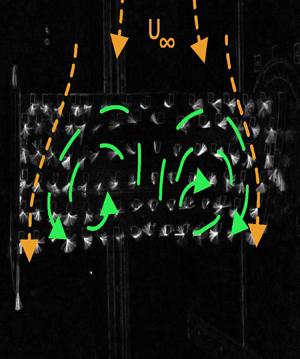
It is possible to identify stall cells from the tuft recordings. The videos have been processed into ensemble images that represent the flow behaviour. First the images are converted to greyscale, shown in figure 3(a). Then to improve the contrast of the tufts, consecutive images from the recording are subtracted. The subtraction can be done by simply shifting the images a single time step forward, and taking the difference at each time step with the original unshifted images. The subtraction eliminates most of the static elements in the images at a short time scale, while preserving the tufts that are unsteady. Next for the investigation of the AR 2.6 wing configuration, 10 subtracted images, sampled linearly across the recorded time frame, are added together to produce the final image. Using more than 10 subtracted images for the final ensemble image can result in the accumulation of noise. The exact number of images to be added together which result in a clear representative result depends on the specific experimental set-up. The set-up used with the AR 5.2 wing for the image acquisition was different and as such 40 images were combined.
Tuft images for the AR 2.6 wing with free stream from left to right. (a) A single frame from a recording showing the original image converted to greyscale. Examples of processed images from recordings for (b) attached flow, (c) separated flow and (d) a stall cell with the relevant flow directions indicated. Orange (dot-dashed line): approximate flow direction outside the stall cell; green (dashed line): approximate flow direction inside the stall cell.

Examples of video recordings processed into a single image are shown in figure 3(b–d) for the main surface flow configurations that have been observed. This processing method allowed for the analysis of several hundred flow cases where distinction is made between: attached flow, separated flow, a single stall cell and two stall cells for the AR 5.2 wing. The separated flow in this case indicates partial or fully separated flow over the wing surface without a persistent preferred surface flow direction over time indicating a stall cell. Typically flow separation starts at the trailing edge as mentioned by Reference Yon and KatzYon and Katz (1998) at lower angles of attack. When the angle of attack is further increased, intermittent flow patterns that extended further towards the leading edge were observed for some combinations of angle of attack, Reynolds number and flap angle. As these flow patterns are not sustained over time they are also considered as separated flow for the purpose of this investigation. In figure 3(d) a single stall cell is shown with the flow direction inside the stall cell indicated by the dashed green line and the flow near the surface outside the stall cell indicated by the orange dot-dashed line. Due to the slight oscillations of the stall cells, the tufts are not steady but do have a preferred flow direction. This results in tufts showing as circle sectors with a sector angle depending on the tuft steadiness and global direction dominated by the local average flow. Although the stall cell patterns can be oscillating slightly in the spanwise direction, they do not appear and disappear over time. The distinctions of the observed flow phases have then been assembled in an  $\alpha \unicode{x2013}Re$ diagram for each flap angle.
The importance of varying either the angle of attack or the Reynolds number to trigger stall cells has not been addressed in previous research. This is potentially relevant due to different instabilities arising from the dynamic change in angle of attack or Reynolds number. Using a constant angle of attack and varying the Reynolds number leads to the change in Reynolds number dominating the creation of a stall cell. Even when the velocity of the wind tunnel is brought to zero between angle-of-attack changes, during wind velocity ramp up the wing will experience a similar Reynolds-number change. Instead it was chosen to vary the angle of attack at a constant Reynolds number. Since the wing is controlled electronically a consistent rate of change in angle of attack is used across the entire experimental campaign. The resulting force data have been processed according to the set-up into the lift coefficient. In figure 7 the 95 % confidence interval for the angle of attack and lift coefficient is shown.
4. Results
4.1 Aspect ratio 5.2 tufts
The flap angle ( $\beta$) of the wing has been set to $0^{\circ }$, $5^{\circ }$ and $10^{\circ }$. These changes in flap angle were deemed to be large enough to have noticeable differences in flow behaviour and force measurements, while not deflecting the flap too much, thereby limiting the effect of the camber line discontinuity at the flap hinge location. The limited flap deflection can thus be assumed to be equivalent to changes in airfoil camber. The tuft results shown here cover a range of angle of attack between $11.4^{\circ }$ and $18.5^{\circ }$ and a Reynolds number range from 100 000 to 510 000. Any of the flow behaviours that have been observed are represented by one of four categories detailed here. The first category, represented by a ‘0’, indicates that no stall cells are observed and the flow is mostly attached such as shown in figure 4(a). The next category represented by a ‘1’ indicates that a single stall cell can be identified on the wing. This can be found with either separated or attached flow on the remainder of the wing span. An example is shown in figure 4(b). Due to the large AR it is also possible for two stall cells to appear on the wing along the span which is indicated by a ‘2’, an example of which is shown in figure 4(c). Furthermore in two cases separated flow across the whole span was observed, which did not exhibit a flow pattern that resembles that of a stall cell anywhere on the wing. These two cases are represented by an ‘s’, one of which is shown in figure 4(d).
Processed tuft images for the AR 2.6 wing with free stream from left to right for different flow topologies: (a) attached flow, (b) a single stall cell, (c) two stall cells and (d) separated flow. Orange (dot-dashed line): approximate flow direction outside the stall cells. Green (dashed line): approximate flow direction inside the stall cells.

In table 1, the observed flow behaviour is shown for the wing with different flap deflections applied. For  $\beta = 0^\circ$, it can be seen that for the lowest Reynolds number of 100 000 initially no stall cell is observed at an angle of attack of 12.8 $^\circ$. Increasing the angle of attack will result in the formation of a stall cell at an angle of attack of 14.2 $^\circ$. Further increasing the angle of attack at a fixed Reynolds number results in the flow fully separating without any stall cell patterns. At higher Reynolds numbers, stall cells tend to form on the wing when the flow separates. The table also shows that for increasing flap angles (i.e. $\beta = 5^\circ$ and $10^\circ$), stall cells occur at similar or lower angles of attack for the same Reynolds number. Furthermore it can be seen that at higher flap angles the flow configuration with two stall cells becomes more prevalent.
Flow behaviour for AR 5.2 for three different flap angles:  $\beta = 0^{\circ }$, $5^{\circ }$ and $10^{\circ }$. The different categories: 0, no stall cells; 1, a single stall cell; 2, two stall cells; s, full-span separated flow.

The initial formation of these stall cells occurs due to the increase of the angle of attack at a constant Reynolds number. As such, the flow behaviour switches from attached flow initially, to a flow configuration with stall cells. This is different from investigations where the Reynolds number is varied at a fixed angle of attack. When the Reynolds number is varied at a fixed angle of attack, the flow tends to switch from separated flow at low Reynolds numbers, to stall cells at higher Reynolds numbers. The work of Reference Dell'Orso and AmitayDell'Orso and Amitay (2018) provides information about the minimum required Reynolds number in order to switch from full-span separation to stall cell configurations. In table 1 this region is not well represented. The switch from attached flow to stall cell configurations is much better represented by the experimental results, but this switch of flow behaviour is not equivalent to the switch from separated flow to stall cell configurations.
These two different cases are characterised by their own respective Reynolds-number ranges. An illustrative diagram has been created, based on the current observations, to indicate the two different boundaries to the angle of attack and Reynolds-number range in which stall cells may occur, as shown in figure 5(a). The stall cell formation angle of attack can be seen to be dependent on the Reynolds number and whether the angle of attack or Reynolds number is changed. In figure 5(a) (left) a distinction between two Reynolds-number ranges is illustrated and linked to the flow behaviour. In this figure the low-Reynolds-number range represents the range in which the wing exhibits separated flow when stalled without creating stall cell flow patterns. The high-Reynolds-number range represents the range in which the wing is likely to show stall cell flow patterns when stalled. From figure 5(a) (left) it can also be seen that changing the angle of attack or the Reynolds number to create stall cells will approach the region in which they exist from different flow regimes. As such, by choosing to vary the angle of attack, the focus is on switching the flow regime from attached flow to stall cells in the high-Reynolds-number range for this wing. The exact position of each flow regime as a function of the angle of attack and Reynolds number is not known for different wings; however, with tuft surface flow visualisation an approximation can be made.
Reynolds number and angle of attack stall cell formation criteria. (a) Left: the indication of the Reynolds number regimes that are relevant for stall cell assessment. Right: approximate range under investigation for the AR 5.2 wing. The arrows indicate the influence of reducing the airfoil camber on stall cell formation criteria. (b) First stall cell occurrence for increasing angle of attack at constant Reynolds number, for AR 5.2.

The switch from fully separated flow to stall cells has only been observed for the wing with a flap angle of  $0^{\circ }$ at the lowest Reynolds number. At higher flap angles all separated flow configurations included stall cell patterns. This indicates that for higher flap angles the flow will tend to switch from separated flow to a stall cell configuration, at lower Reynolds numbers than have been tested. Therefore in the low-Reynolds-number regime, less camber potentially leads to a delay in the formation of stall cells to higher Reynolds numbers, at a fixed angle of attack. The switch from attached flow to stall cell configurations is represented in more detail by the tuft results.
The initial angle of attack at which stall cells form for a fixed Reynolds number is visualised in figure 5(b) for the different flap angles that have been tested. In this high-Reynolds-number range, less camber tends to postpone the formation of stall cells to larger angles of attack. This is an approximation of the boundary (formation criteria) between attached flow and stall cells. The large angle-of-attack step size for the AR  $5.2$ wing results in rather discrete measurements with regards to the observation of stall cell formation. In figure 5(b) it can be seen that the required angle of attack for initial stall cell formation decreases or stays the same, for increasing flap angles at a fixed Reynolds number. In figure 5(a) (right) the relevant region that has been observed with the tufts is illustrated, showing the effect of decreasing camber with arrows on the formation criteria of a stall cell.
With a broad overview of camber effects on stall cell formation, further tuft visualisation and force measurements were carried out with the AR  $2.6$ wing. For this AR, only a single stall cell will form over the surface; however, we will also be able to directly measure the forces experienced by the wing and relate those to the stall structure (since there is no support at the other end of the wing for our wind tunnel configuration). These results are presented in the following sections.
4.2 Aspect ratio 2.6 tufts
The reduction of the AR of the wing allows for an investigation of the flow behaviour of a single stall cell. The method of identifying flow behaviour with tufts is employed again. In figure 3 the resulting processed images from the tuft recordings for the AR 2.6 wing are shown for the three categories of flow behaviour that have been observed on this wing. These categories of flow behaviour are also used in the flow behaviour diagrams in this section. In these diagrams (figure 6a–c) attached flow is represented by a green triangle, separated flow by a red diamond and a stall cell by a blue circle. Attached flow also includes some trailing-edge unsteadiness, but no upstream flow. Separated flow for the AR 2.6 wing includes trailing-edge separation and intermittent separated flow patterns. Cases indicated as stall cells show a clearly defined stall cell flow pattern which is persistent over time.
Flow behaviour for AR 2.6 at three different flap angles: (a)  $\beta = 0^\circ$, (b) $\beta = 5^\circ$ and (c) $\beta = 10^\circ$. The different symbols show different flow topologies: attached flow, triangle; separated flow, diamond; stall cell, circle. (d) The angle of attack at which the first stall cell occurs at constant Reynolds number for different flap angles (in the high-Reynolds-number regime), for AR 2.6.

The results from the tuft observations are summarised in three diagrams, one for each flap angle. The first diagram showing the flow behaviour for a flap angle of  $0^{\circ }$ is shown in figure 6(a). In the flow behaviour diagrams the angle of attack at maximum lift coefficient is indicated with a black dashed line. Two observations in figure 6(a) can be made in comparison with the results from the AR 5.2 wing in table 1. First, the minimum required Reynolds number for stall cell formation in the low-Reynolds-number regime is no longer observable; stall cells are already present at the lowest Reynolds number tested. This contradicts the observations made by Reference Dell'Orso and AmitayDell'Orso and Amitay (2018) where it was observed that the minimum required Reynolds number increases with decreasing AR. However, the results for the AR 5.2 wing have been obtained in a two-dimensional configuration, whereas the AR 2.6 wing used an endplate at the wing tip which only partially eliminated the three-dimensional effects. A displaced tip vortex at the edge of the endplate might still have an influence on the flow near the wing tip. It is unknown as to what the influence of the three-dimensional effects is on the stall cell formation criteria, and therefore it is not possible to make an assessment of the influence of the AR on the formation criteria such as presented here. The results for the AR 2.6 wing will thus only be compared with each other and not with those for the AR 5.2 wing investigation. Next it can be observed in figure 6(a) that between attached flow (green triangles) and stall cells (blue circles) there is a small range of angle of attack in which the flow is separated (red diamonds). Similar observations have been described by Reference Yon and KatzYon and Katz (1998) who also found a range of a few degrees of angle of attack beyond maximum lift in which flow separation develops prior to stall cell formation. This flow separation was not noticed in the AR 5.2 wing experiments due to the large step size for the angle of attack.
For the AR 2.6 wing, the minimum required angle of attack for stall cell formation in the high-Reynolds-number regime is shown in figure 6(d). The data points used for this graph are the first occurrences of stall cells by varying the angle of attack at a fixed Reynolds number. The graph confirms the observation made earlier for the AR 5.2 wing in the high-Reynolds-number regime. It can be seen that reducing the flap angle tends to postpone the formation of stall cells to larger angles of attack at a fixed Reynolds number. For the cases with flap angle of  $5^{\circ }$ and Reynolds number between $3.0 \times 10^5$ and $4.0 \times 10^5$ (two cases) the first stall cells form at angles of attack which are lower than what might be expected from the other observations. For these cases the range of angle of attack in which some form of flow separation occurs prior to the formation of stall cells can be seen to be smaller in figure 6(b).
4.3 Aspect ratio 2.6 lift coefficient
The lift of the AR 2.6 wing has been measured during the tuft observations and allows one to link wing performance to visually identified flow behaviour. An endplate was used to ensure that the influence of a tip vortex is limited on the formation of stall cells. This invariably has an effect on the lift coefficient; however, this is not critical for the results/discussion in this section as the comparisons are made between different flap angles for the same AR. Figure 7 shows the lift coefficient around stall for the three flap angles that have been tested. As the stall cells locally influence the surface pressure, they will also have an effect on the lift generated by the wing. For the lift coefficient analysis only the AR 2.6 wing is used, as the limited AR allows for only a single stall cell.
Lift coefficient with 95 % confidence bounds and initial stall cell formation angle of attack indicated by diamonds for (a)  $\beta = 0^\circ$, (b) $\beta = 5^\circ$ and (c) $\beta = 10^\circ$.

Describing the formation criteria of stall cells in terms of angle of attack and Reynolds number is not ideal as it has been shown to not reflect the airfoil shape. The lift coefficient polars take into account the angle of attack, airfoil shape and Reynolds number. The direct influence of stall cells on the pressure coefficient further provides reason to link the lift coefficient to stall cells. Reference Gross, Fasel and GasterGross et al. (2015) provide a model to calculate the spanwise spacing of stall cells from the local lift polar gradient of an infinite wing in the range where stall cells occur. The model is represented as follows:
 \begin{equation} \frac{L}{c} = {-}\frac{\rm \pi}{4} \times \frac{\delta C_L}{\delta \alpha}, \end{equation}
where  $L/c$ refers to the spanwise periodic spacing of stall cells and $\delta C_L$/ $\delta \alpha$ to the local lift polar gradient in the range of stall cell formation. This model can also be used to predict the local lift curve gradient in the range of stall cell formation if the relevant stall cell spacing is known. If the corresponding lift curve is available, the angle of attack for stall cell formation can be estimated. The proposed model by Reference Gross, Fasel and GasterGross et al. (2015) has the possibility of taking into account the airfoil shape in the prediction of the stall cell angle of attack. If there is an influence on the stall cell spacing due to the airfoil shape, then this will also affect the predicted lift polar gradient output. Furthermore the fixed local lift polar gradient for a certain stall cell spacing, as predicted by the model, still yields different angles of attack for stall cell formation in combination with different lift polars.
From the tuft results for the AR 5.2 wing it was shown that the wing can accommodate two whole stall cells along the full span. When using the AR 2.6 wing, a single whole stall cell has been observed. Changing the flap angle has shown no change in the maximum amount of stall cells on the wing span. These observations indicate that the (periodic) spanwise spacing of the stall cells under investigation can be assumed to be equivalent to the AR (i.e. 2.6). In combination with (4.1), the predicted local gradient at stall cell formation can be found to be  $-3.31$ rad $^{-1}$, which is an approximation for an infinite wing applied to the current case which uses an endplate.
The use of the predicted local lift polar gradient in combination with the known lift polars allows for the estimation of the angle at which stall cells occur. However, not all obtained lift polars have local gradients that match or exceed the predicted local gradient; this is shown by figure 8. The local gradient predicted by the model from Reference Gross, Fasel and GasterGross et al. (2015) (horizontal dashed line) comes close to the observed local minimum gradient after stall for most observations at lower Reynolds numbers. Due to the presence of measurement noise in the experimental data, the resulting local gradient from the lift polars is neither smooth or monotonically decreasing. This further complicates an estimate of the angle of attack at which the local lift polar gradient has a specified value of  $-3.31$ rad $^{-1}$. Instead a best approximation with the current data has been made by estimating the angle-of-attack range within which most the local gradients approximate as $-3.31$ rad $^{-1}$. A few degrees after stall, within a range of approximately $1^{\circ }$, this can often be observed. This range is indicated by the two thin vertical lines in figure 8. The average of this range, estimated to be 14.5 $^\circ$, is shown by the thick vertical line in figure 8. This is the angle of attack at which the local lift polar gradient approximates as $-3.31$ rad $^{-1}$ and thus stall cells would likely occur.
Symbols: the local gradient obtained from the lift polars (for the AR 2.6 wing) with a central difference scheme. Horizontal dashed line: gradient obtained from the model of Reference Gross, Fasel and GasterGross et al. (2015). Vertical dot-dashed lines: approximation of the range for stall cell formation.

The constant angle-of-attack estimation for the formation of stall cells as motivated by the model of Reference Gross, Fasel and GasterGross et al. (2015) can be compared with the known angle of attack for stall cell formation to provide an error. The mean absolute error (MAE) is used which allows direct interpretation of the error as the average deviation from the true value. Additionally the flap angle and Reynolds number play a role, and, as such, two sets of results are presented. In figure 10(a) the error as a function of the Reynolds number is shown. The results from the method of Reference Gross, Fasel and GasterGross et al. (2015) (blue crosses) show relatively little change in error over the tested Reynolds-number range, with the exception of the lowest Reynolds number. When observing the error as a function of the flap angle, such as shown in figure 10(b), it can be seen that the error tends to decrease for larger flap angles.
Further options to predict the angle of attack at which stall cells form can be formulated based on the available data. The stall angle is chosen as a reference point from where the angle at which stall cells occur is calculated. The reason for this is that the stall angle takes into account both Reynolds-number effects and the airfoil shape. The stall angle is smaller than the angle at which stall cells occur, resulting in  ${\rm \Delta} \alpha$ such as shown in figure 9(a).
Difference  ${\rm \Delta} C_L$ as a parameter for stall cell investigation. (a) Lift coefficient obtained in the wind tunnel, using ${\rm \Delta} C_L = C_{L,max} - C_{L,SC}$ for estimation of stall cell formation. (b) Difference between maximum $C_L$ and $C_L$ at which stall cells appear when increasing the angle of attack at a fixed Reynolds number. Linear fit: ${\rm \Delta} C_L = 0.017 \times Re + 0.036$.

Parameter  ${\rm \Delta} \alpha$ in combination with the lift polar results in a corresponding ${\rm \Delta} C_L$ over the ${\rm \Delta} \alpha$ range, and an average gradient between the stall angle and the angle at which stall cells form. The ${\rm \Delta} C_L$ such as shown in figure 9(a) can be calculated from the lift polars and tuft observations for the AR 2.6 wing under investigation. The result is shown in figure 9(b). The observations in figure 9(b) consider both the lift coefficient at maximum lift and the lift coefficient at initial stall cell formation. These conditions can be influenced by small disturbances such as for example the Crow-like instability, the turbulence intensity, the surface finish and potentially many more. Specifically at lower Reynolds numbers (below $4 \times 10^5$ in this case) the results can be more scattered. With the current or previous investigations it is not possible to conclusively indicate the cause for the scatter. With SOFV (Reference Dell'Orso and AmitayDell'Orso & Amitay, 2018) were able to illustrate that near the onset of stall cell formation, the surface flow patterns potentially exhibit bi-stable flow patterns or previously undefined flow patterns between full separation and stall cells. It is possible that, as a result, the range of potential ${\rm \Delta} C_L$ at lower Reynolds numbers tested here is larger. Multiple repetitions of the experiment would be required to determine the possible range of ${\rm \Delta} C_L$ as obtained from the force measurements and tufts. Instead it was chosen to cover many different cases; as such, a linear fit to all the observations is also included. The linear fit is a first-order approximation of a potentially higher-order relation between ${\rm \Delta} C_L$ and the Reynolds number. The first-order approximation illustrates how the drop in lift coefficient between maximum lift and the onset of stall cells tends to increase at higher Reynolds numbers. Using an approximation for ${\rm \Delta} C_L$ in combination with the post-stall lift curve gradient (between stall and stall cell formation) and the angle of attack at maximum lift, an approximation for the angle of attack at which stall cells occur can be found. The linear formula is shown by (4.2). As both the stall angle and the post-stall lift polar gradient can be obtained from the lift polar, getting an accurate angle-of-attack estimation for stall cell formation depends on estimating ${\rm \Delta} C_L$ in (4.2):
 \begin{equation} \alpha_{SC} = \alpha_{C_{L,max}} - \left( \frac{{\rm d} \alpha}{{\rm d} C_L} \right)_{PS} \times {\rm \Delta} C_L.\end{equation}
 In figure 9(b) the  ${\rm \Delta} C_L$ values can be seen to range between approximately 0.03 and 0.15; the average can be found to be approximately 0.088. Using this value as a constant ${\rm \Delta} C_L$ in combination with (4.2) and the different lift polars that have been obtained, allows for the estimation of the angle of attack at which stall cells form. The error from the resulting estimation is shown by the red squares in figures 10(a) and 10(b). The error is relatively inconsistent across the Reynolds-number range compared with the method of Reference Gross, Fasel and GasterGross et al. (2015). In order to further compare the results, the error statistics across all observations are given in table 2. The resulting MAE and standard deviation of the absolute error of both the method based on Reference Gross, Fasel and GasterGross et al. (2015) and using a constant ${\rm \Delta} C_L$ estimate are very close.
The MAE for the predicted angle of attack at which stall cells form. (a) Averaged flap angle results for each Reynolds number. (b) Averaged Reynolds number results for each flap angle.

The MAE and the standard deviation of the absolute error for the predicted angle of attack at which stall cells form, for three flap angles at nine different Reynolds numbers (27 cases total).

From the available data and (4.2) it follows that an improved  ${\rm \Delta} C_L$ estimate directly improves the estimation of the corresponding angle of attack for stall cell formation. Therefore the linear fit such as shown in figure 9(b) can be used. The resulting ${\rm \Delta} C_L$ from this linear fit is a function of the Reynolds number, but does not directly take into account the flap angle. However, just as before, the resulting ${\rm \Delta} C_L$ is applied to each lift polar individually which is dependent on the flap angle and Reynolds number. Assuming this linear relationship, the error of the resulting prediction of the angle of attack for stall cell formation is shown by the yellow circles in figures 10(a) and 10(b). Significant improvements across the Reynolds-number range can be observed with the exception of the range close to the average Reynolds number. This is due to the average ${\rm \Delta} C_L$ (as used previously) being equivalent to ${\rm \Delta} C_L$ obtained from the linear fit with the average Reynolds number. This is expected due to the limitation of the fitting process.
The error statistics of the method which uses a linear fit of  ${\rm \Delta} C_L$ as a function of the Reynolds number are also presented in table 2. Using the ${\rm \Delta} C_L$ approximation dependent on the Reynolds number, but independent of the flap angle, results in a MAE of 0.58 $^\circ$. Clearly, significant improvements can be made by estimating ${\rm \Delta} C_L$ with a linear fit (rather than assume a constant value of ${\rm \Delta} C_L$). Finally, it should be noted that a linear fit is used here not with any physical reasoning, but to capture the trend in the data. If there are more data (over larger range of Reynolds numbers and different airfoil shapes), then a multi-parameter fit could be used to further improve the predictive capabilities. In fact, a larger dataset could be coupled with advanced curve-fitting tools (such as machine learning) to further improve the predictive capabilities.
5. Conclusions
The requirements for stall cells to occur on a wing with trailing-edge stall focus on finding the minimum required angle of attack and Reynolds number, for a specific airfoil profile and experimental set-up. In this work the Reynolds number has been varied in a range of 100 000 to 500 000 and the angle of attack from before stall to approximately 10 $^\circ$ after stall. These parameters have been investigated for a NACA0012 wing with a trailing-edge flap. Changes in the flap angle (0 $^\circ$, 5 $^\circ$, 10 $^\circ$) provide an estimate for the influence of the airfoil profile on the stall cell formation criteria. Tufts have been used to identify the flow behaviour near the wing surface. The results from the tuft investigations have shown that when assessing the requirements for stall cell formation, two different Reynolds-number regimes exist. The low-Reynolds-number regime, below a Reynolds number of approximately 150 000 for the two-dimensional case tested, considers the transition from separated flow to stall cells and in this regime the Reynolds number is dominant. A high-Reynolds-number regime can be observed above a Reynolds number of approximately 150 000 for the two-dimensional case tested, when the flow switches from attached flow to stall cells with only a minor angle-of-attack range with separated flow between. In the high-Reynolds-number range the change in angle of attack is dominant for the flow behaviour. Preliminary observations have indicated that in the low-Reynolds-number regime the formation of stall cells is postponed to higher Reynolds numbers by reducing the airfoil camber. In the high-Reynolds-number regime it is expected that the reduction of camber postpones the formation of stall cells to higher angles of attack.
The effects of Reynolds number on the lift coefficient are suspected to be correlated with the flow behaviour that has been observed on the wing. A method which relates the stall cell spacing and the lift-curve slope from Reference Gross, Fasel and GasterGross et al. (2015) has been used to estimate the angle of attack at which stall cells form, based on angle of attack versus lift coefficient curves. Further estimates for the angle of attack at which stall cells form have been formulated based on the lift coefficient and known observations. The method of Reference Gross, Fasel and GasterGross et al. (2015) and the empirical method provide a first step towards estimating stall cell formation from average lift coefficient measurements. In addition to the practical use, this indicates the importance of the lift coefficient for stall cell investigations. Further investigations should validate the current findings on wings with different sectional profiles, and this will be the subject of our future work.
Funding
The authors gratefully acknowledge funding from H2020 Project HOMER (project no. 769237) and EPSRC (grant ref. EP/R010900/1).
Declaration of interests
The authors declare no conflict of interest.
Author contributions
Conceptualisation: F.D.V. and B.G.; investigation: F.D.V.; writing original draft: F.D.V.; writing review and editing: B.G.
Data statement
All data supporting this study, including supplementary material, are openly available via the University of Southampton repository at https://doi.org/10.5258/SOTON/D2210.
Ethical standards
The research meets all ethical guidelines, including adherence to the legal requirements of the study country.
A. Appendix. Further experimental details
The experimental set-up and methodology described in §§ 2 and 3 provide an overview of the relevant steps for the current investigation and a general experimental set-up. Due to the specifics of the current set-up used, further care has been taken to account for small deviations in the angle of attack, the repeatability of the measurements has been evaluated and an assessment of the tip vortex influence at the endplate has been made. These aspects and other elements which are relevant to stall cells are described here.
Stall cells tend to be sensitive to multiple aspects of the experimental set-up, such as the turbulence intensity, surface finish, the exact AR and many more factors. In the current investigation, the factors outside of the tested parameters which influence stall cells are mostly constant, as the experimental set-up does not change. The experimental lift coefficient data for the wing with AR of 2.6 were acquired by increasing the angle of attack at a fixed Reynolds number and flap angle. For each Reynolds number and flap angle combination, two angle-of-attack sweeps have been performed. The use of two angle-of-attack sweeps allows an assessment of the repeatability of the measurements as the flow under consideration is highly turbulent. In order to limit the required wind tunnel time, the two angle-of-attack sweeps use an offset in the set angle of attack. The first sweep considers integer set angles [ $\ldots,10,11,12,\ldots$]; the second sweep uses a $0.5^{\circ }$ offset for the set angles of attack [ $\ldots,10.5,11.5,12.5,\ldots$]. The use of two distinct sweeps allows an evaluation of the consistency of the results for a large number of cases with an approximately $0.5^{\circ }$ step size in angle of attack, while minimising the necessary wind tunnel time. It should be noted that in industrial applications, wind tunnel time availability is a critical component of decision making in terms of data acquired.
In figure 11 the data are shown from the raw measurements of the lift coefficient at the set angles of attack by the filled circles. From the data, specifically at lower Reynolds numbers, it can be seen that the successive angle-of-attack measurements are from alternating sweeps through the consistent lift coefficient difference they have over the range of angles of attack measured. At higher angles of attack and Reynolds numbers the difference between the two sweeps fades away and the measurements around and after stall become more consistent. At the lower Reynolds numbers the differences are likely attributable to the exact geometry of flow configuration of the stall cell that is triggered. Once a stall cell has appeared it was found to persist throughout the rest of the angle-of-attack sweep. The discrepancy between the two angle-of-attack sweeps is not uncommon and is similar to that of Reference Gregory and O'ReillyGregory and O'Reilly (1970) who show a comparable deviation between lift coefficient measurements of a NACA0012 wing profile at a Reynolds number of  $0.46 \times 10^6$ which is close to the highest Reynolds tested in the current investigation. An investigation by Reference Bartl, Sagmo, Bracchi and SætranBartl et al. (2019) focused on quantifying the performance of an airfoil section; however, results from different set-ups with the same airfoil section yielded very different results near and after stall. Although Reference Bartl, Sagmo, Bracchi and SætranBartl et al. (2019) attribute some of the stark differences to the change in AR and turbulence intensity potentially, these factors are directly related to the formation of stall cells and their characteristics. The investigation by Reference Dell'Orso and AmitayDell'Orso and Amitay (2018) documents the large amount of flow configurations that can exist in a similar range of Reynolds-number and angle-of-attack combinations, specifically when the flow parameters are in the domain where stall cells initially form. Still, from the current investigation it can be noticed that even two different angle-of-attack sweeps with a small lift coefficient offset do retain a similar lift polar gradient after stall, as shown in figure 11, indicating that the change in flow behaviour influence on the lift coefficient as caused by the increasing angle of attack is consistent regardless of the initially created stall cell on the wing surface. In order to represent the gradient as observed in each sweep individually as a single dataset, the moving mean between two consecutive samples has been taken, resulting in the dashed line with local averaged data points indicated by open circles in figure 11.
Raw lift coefficient measurements (filled circles) for a set angle of attack and the moving average (open circles with dashed line) for (a)  $\beta = 0^\circ$, (b) $\beta = 5^\circ$ and (c) $\beta = 10^\circ$.

Measurements of the lift force were taken with the tufts on the wing, while the wing was supported on only one end and used the endplate on the free end. The wing angle of attack was calibrated using the linear lift coefficient region during testing, to approximate the true angle of attack of the wing in the wind tunnel with the set angle of attack. After testing, the resulting data have been used to check this calibration and all cases are corrected once again to eliminate small calibration errors. Finally it was noticed that the stepper motor which is directly attached to the quarter chord line of the wing to control the angle of attack is not perfectly fixed for any angle of attack but can deviate slightly due to a lack of holding torque. During the experiments it was observed that at the highest induced wing-pitching moment, the angle of attack could deviate by  $1^{\circ }$ from the set angle of attack in the direction of the pitching moment. The stepper motor angular displacement has been approximated as a linear torsional spring with a deviation of $1^{\circ }$ at the maximum measured pitching moment induced by the wing. The measured moment for each case has then been used to correct for any small angle-of-attack deviations caused by the stepper motor. These corrections have been implemented to result in the data as shown in figure 7.
The use of the endplate for the unsupported end of the wing with AR of 2.6 is only partially effective at eliminating tip vortex effects. From the linear region of the NACA0012 profile with endplate and without flap deflection, a lift-curve gradient of approximately  $1.2 {\rm \pi}$ can be found (also shown in figure 8), indicating the deviation from the theoretical two-dimensional performance. The maximum lift coefficient at a Reynolds number of $0.46 \times 10^6$ was found at an angle of attack of approximately $13.5^{\circ }$ for the two-dimensional configuration used by Reference Gregory and O'ReillyGregory and O'Reilly (1970), whereas for the current investigation the maximum lift coefficient was found at an angle of attack of approximately $14.25^{\circ }$. This is certainly a limitation but it does not take away from the conclusions of this case study. Moreover, preliminary PIV measurements taken in the wake of the wing at a constant Reynolds number and angle of attack at three different flap angles showed almost no difference in the tip-vortex-induced spanwise velocity at the endplate.
Finally, some observations with regards to stall cells can be made which do not contribute to the general analysis discussed, but hold relevance to the wider body of literature regarding stall cells. In some investigations stall cells have been described as unsteady; this can refer to both the existence of a stall cell or the position of a stall cell over time. In the current investigation the unsteady existence of stall cells was observed prior to the formation of a complete clearly distinguishable stall cell. Typically flow separation occurs near the trailing edge first and extends further upstream as the angle of attack is increased. Further increasing the angle of attack can produce intermittent flow patterns which take on a variety of flow configurations among which are also stall cells with approximately half the width of the stable stall cell patterns. Both the trailing-edge separation and cases with intermittent flow patterns are classified as separated flow for the analysis of the AR 2.6 wing. At higher angles of attack than for trailing-edge separation or intermittent separation, stall cells form which persist over time and hold a consistent flow pattern across the span of the wing. These stall cells have been found to oscillate only slightly in the spanwise direction. This is potentially a consequence of the span being nearly equal to the width of the stall cell.


 Open access