


Impact Statement
This paper presents methodology to evaluate competing probabilistic forecasts for engineering operations. It summarizes the relevant statistical literature for an engineering audience. A case study is presented on which engineering operators may emulate their own forecast evaluation process. All authors have experience working with maritime engineering industry and know the methods described within to be necessary to operations.
1. Introduction
Recent advances in technology and the availability of data acquisition devices have increased the role of the data sciences in maritime engineering. In the past, smaller datasets produced by experimental laboratories were used to answer questions such as the effect of extreme loadings on the remaining useful life of an asset. Now, in addition to experimental data, large near-real-time operator-acquired data have the potential to aid asset management, condition health monitoring, safety and risk, and other aspects of day-to-day operations. One of the most useful consequences of increased data capture is the availability to maritime operations of enhanced forecasting products. However, the data campaigns used to support forecasting and other data-driven activities are often costly and may involve negotiating hostile or isolated environments, require maintenance of data capture devices in harsh environments, and necessitate the building of new communication infrastructure. For example, to install, maintain, and record data from a single mooring monitor on the Exmouth Plateau for a year costs around AUD1,000,000 (Astfalck et al., Reference Astfalck, Cripps, Gosling, Hodkiewicz and Milne2018). To justify the significant cost and effort required to install and maintain advanced measurement technology in marine environments, the contributed value of the data to the operator deserves to be rigorously assessed.
Even with careful data collection, marine data can remain uncertain, as can the physics underlying offshore numerical forecasting models. Decisions based on forecasts often benefit from a probabilistic quantification of these sources of uncertainty, but model selection and inference can be complex. The translation of results from statistician to end user is also a challenge: to establish trust in a decision support tool, the process must be targeted, transparent, and readily accessible. Forecasting of physical systems has historically been domininated by deterministic approaches in which the future state is assumed to be determined given a known initial state and assumed future forcings (Anderson Loake et al., Reference Anderson Loake, Astfalck and Cripps2022). However, in reality, all observed data are a noisy representation of a true underlying process, initial states of complex systems are rarely known exactly, future forcings are uncertain, and the physics embedded in the numerical forecasting models do not always capture the complexity of the true underlying process. Even when the physics are well understood, they are seldom analytically tractable and therefore require approximate numerical solutions. Acknowledgement of these uncertainties has led naturally to interest in probabilistic forecasting, but for much of the past century the role of probability in forecasting complex systems was limited by complications stemming from nonstandard data, complex nonlinear physical relationships, computational demands, and large domains over which we wished to quantify uncertainty (Booker and Ross, Reference Booker and Ross2011). With increased computational capacity and the advent of numerical integration techniques such as Markov chain Monte Carlo (MCMC), this century has seen a marked increase of probabilistic techniques for forecasting (Gneiting and Katzfuss, Reference Gneiting and Katzfuss2014).
Forecasting products have become vital to offshore engineering operations. Forecasts have been produced for future meteorological and oceanographic states (Schiller et al., Reference Schiller, Brassington, Oke, Cahill, Divakaran, Entel, Freeman, Griffin, Herzfeld, Hoeke, Huang, Jones, King, Parker, Pitman, Rosebrock, Sweeney, Taylor, Thatcher, Woodham and Zhong2020), structural responses (Zhao et al., Reference Zhao, Milne, Efthymiou, Wolgamot, Draper, Taylor and Taylor2018a; Astfalck et al., Reference Astfalck, Cripps, Gosling and Milne2019a), and energy demands (Foley et al., Reference Foley, Leahy, Marvuglia and McKeogh2012). Broadly, engineers categorize forecasting models as either numerical, data-only, or hybrid (Sikorska et al., Reference Sikorska, Hodkiewicz and Ma2011). Numerical models represent the underlying physics of a system and calculate the propagation of the physical states, data-only models find structure in the observed data that may be used to predict future states, and hybrid models incorporate both numerical and data-only techniques. With the increasing volume of data that are being measured, and the development of technologies that allow rapid propagation of uncertainty through computationally demanding maritime models such as statistical emulation (Astfalck et al., Reference Astfalck, Cripps, Hodkiewicz and Milne2019b) and digital twins (Ward et al., Reference Ward, Choudhary, Gregory, Jans-Singh and Girolami2021; Jorgensen et al., Reference Jorgensen, Hodkiewicz, Cripps and Hassan2023), the value of probabilistic forecasting in engineering operations is being recognized (see, for instance, Pinson, Reference Pinson2013 and Anderson Loake et al., Reference Anderson Loake, Astfalck and Cripps2022). In practice, there is often a plurality of competing forecasts, often at the expense of paying third-party contractors or maintaining measurement equipment to record data required by statistical or machine learning methods. The standard practice in industry is to evaluate these forecasts by distance-based metrics (such as squared or absolute error). When provided with a probabilistic forecast, a distance is generally defined between the observed data and a point measure of forecast centrality such as the mean. Under a distance-based metric, forecasts with identical point measures (e.g., mean) but different uncertainties (e.g., variance) receive the same score. Thus, critical aspects of the forecasts are ignored by these metrics and so they may not entirely or fairly assess forecast performance. Therefore, there is a need for a consistent and transparent theory with which to judge, rank, and ultimately select a forecasting product for operations. Such a theory can be used to evaluate the quality of forecasts before the model is deployed to select a model and build operator confidence, but also afterwards, so that any deterioration in performance can be identified.
A theory suitable for judging probabilistic forecasts is found in the statistical literature on proper scoring rules. Proper scoring rules attribute scores to forecasting models to evaluate their performance (see Winkler, Reference Winkler1969 for an early account and Gneiting and Katzfuss, Reference Gneiting and Katzfuss2014 for a recent review). As with many transdisciplinary endeavors, the translation of technical jargon between disciplines is paramount to success. Scoring rule theory is stringent and its literature can be exacting for users who were not trained in statistics, and we believe this is why it is not more commonly referred to in applied fields. Proper scoring rules are formal methods that evaluate forecasting performance by quantifying the forecast sharpness and calibration. They are defined so that a model score is optimized when the true belief of the forecast data is reported by the forecasting model. Scoring rules assess the performance of the forecast by calculating a numerical value; this is convenient when aggregating repeated observations from a forecasting model or for assessing model performance over a prediction domain. We note that alternative graphical methods are also available for assessing the calibration of probabilistic forecasts—for example, Q–Q plots and worm plots (Buuren and Fredriks, Reference Buuren and Fredriks2001) and Talagrand diagrams or rank histograms (Gneiting et al., Reference Gneiting, Stanberry, Grimit, Held and Johnson2008).
End users of forecasting products are not always statistically trained, nor are they always subject matter experts in the science that underpins the forecast. To instill confidence in the decision process, the score attributed to a forecast should be easily interpreted (Bitner-Gregersen and Magnusson, Reference Bitner-Gregersen and Magnusson2014). To this end, we extract from the theory of proper scoring rules (Gneiting et al., Reference Gneiting, Balabdaoui and Raftery2007; Gneiting and Raftery, Reference Gneiting and Raftery2007) three simple and interpretable metrics called the squared error (SE), the Dawid–Sebastiani score (DSS), and the energy score (ES). When assessed together, these metrics provide a robust picture of forecast quality. The three metrics score forecasts on the accuracy of the predictive means, the accuracy of the predictive means accounting for the predictive variance, and the agreement between the observed data and the cumulative distribution functions (CDFs) of the forecasts. Forecasts are often made over a predictive domain such as time (e.g., prediction of a discrete number of future time-steps) or space (e.g., prediction of a continuous spatial process). We show how scoring rules may be defined and calculated as a function of times or locations in a predictive domain and how we may build assessments of forecast model performance to guide decision making.
To exemplify the presented theory, we present a case study of forecast evaluation with surface winds at a location in Australia’s North–West Shelf (NWS), an area of intense maritime operations. The data are measured atop a vessel, whose operations are highly dependent on its immediate meteorological and oceanographic environment. Deterministic numerical forecasts are provided by a third-party forecasting agency and we use these and the observed wind data to build several probabilistic forecasting models. Numerical forecasts are provided at hourly time-steps over a 120-hr prediction horizon. A model output statistics (MOS) model (Glahn and Lowry, Reference Glahn and Lowry1972) is built to scale and rotate the numerical forecast and quantify the forecast uncertainty, and a vector auto-regressive (VAR) model (Shumway et al., Reference Shumway, Stoffer and Stoffer2000) is built on the observed data. We show how calibration of the probabilistic models may be assessed with the use of proper scores. Defining the scores as a function of the prediction horizon exemplifies the strengths and limitations of the hybrid physics/data MOS model against the data-driven VAR model. The data and processes used in this case study stem from a real industry application and are part of a larger research endeavor to quantify uncertainty in a complex engineering environment aboard an asset in Australia’s NWS.
The rest of the paper is structured as follows. Section 2 introduces the statistical theory of proper scoring rules and gives notation for evaluating models over a predictive domain. Section 3 develops the panel of scoring rules that, when assessed together, provide a clear appraisal of forecasting model performance. Section 4 presents a case study of the scoring rules to forecasts for surface winds at a location in Australia’s NWS. Section 5 concludes the paper with a discussion. Code for all methods described in the paper is available at github.com/TIDE-ITRH/scoringrules.
2. Evaluating Forecasts
This section presents a primer on scoring rule theory (Gneiting et al., Reference Gneiting, Balabdaoui and Raftery2007; Gneiting and Raftery, Reference Gneiting and Raftery2007). We define the concept of a prediction space, define proper scoring rules, present methods that may be used to evaluate overall forecasting model performance, and extend the definition of scoring rules over a predictive domain. To firm ideas, we discuss these notions with respect to the case study presented in Section 4.
2.1. Prediction spaces
The prediction space is the fundamental unit of information with which we establish a “score” for a forecasting model. First introduced by Murphy and Winkler (Reference Murphy and Winkler1987), and later extended (and named) by Gneiting and Ranjan (Reference Gneiting and Ranjan2013), a prediction space is a probability space of the joint distribution of a probabilistic forecast $ F $
and an observed data point
$ F $
and an observed data point $ {y}^{\ast } $
. The forecast
$ {y}^{\ast } $
. The forecast $ F $
is a probability distribution specified through a CDF. We then define a prediction space as the collection
$ F $
is a probability distribution specified through a CDF. We then define a prediction space as the collection $ \left(F,{y}^{\ast}\right) $
; simply put, we require the forecast and the observed data to calculate a score for the forecasting model (see Gneiting and Ranjan, Reference Gneiting and Ranjan2013 for a rigorous mathematical definition). The forecast
$ \left(F,{y}^{\ast}\right) $
; simply put, we require the forecast and the observed data to calculate a score for the forecasting model (see Gneiting and Ranjan, Reference Gneiting and Ranjan2013 for a rigorous mathematical definition). The forecast $ F $
is conditioned on all available and pertinent observations, beliefs, and physics; here, we represent this information by
$ F $
is conditioned on all available and pertinent observations, beliefs, and physics; here, we represent this information by $ \mathcal{A} $
. For example,
$ \mathcal{A} $
. For example, $ \mathcal{A} $
could contain covariates, model assumptions, or physical scientific relationships. Before we observe
$ \mathcal{A} $
could contain covariates, model assumptions, or physical scientific relationships. Before we observe $ {y}^{\ast } $
, we say that the true distribution
$ {y}^{\ast } $
, we say that the true distribution $ p\left({y}^{\ast }|\mathcal{A}\right) $
(i.e., the true distribution of
$ p\left({y}^{\ast }|\mathcal{A}\right) $
(i.e., the true distribution of $ {y}^{\ast } $
conditioned on information
$ {y}^{\ast } $
conditioned on information $ \mathcal{A} $
) is the ideal forecast relative to
$ \mathcal{A} $
) is the ideal forecast relative to $ \mathcal{A} $
.
$ \mathcal{A} $
.
2.2. Proper scoring rules
Scoring rules attribute a numerical value $ S\left(F,{y}^{\ast}\right) $
to a prediction space
$ S\left(F,{y}^{\ast}\right) $
to a prediction space $ \left(F,{y}^{\ast}\right) $
and are constructed to maximize the sharpness of the forecast distribution, subject to calibration of the forecast with the observations. Here, sharpness is inversely related to forecast variance (maximizing sharpness minimizes the predictive variance), and calibration is a metric of the agreement of the probabilistic forecasts and the observations (Murphy and Winkler, Reference Murphy and Winkler1987). Sharpness is a function of the forecast alone, while calibration is a function of the forecast and the observations. The concepts of sharpness and calibration in statistics are akin to precision and accuracy in engineering, where precision is a measure of dispersion, and accuracy is both a measure of trueness (i.e., the distance between an observed point and its forecast value) and precision (ISO 5725-1:1994, 1994). Further note that the term calibration is overloaded between the statistics literature (as defined above) and the engineering literature (where it is defined in terms of honing a measurement instrument or numerical model); we use the statistics definition herein.
$ \left(F,{y}^{\ast}\right) $
and are constructed to maximize the sharpness of the forecast distribution, subject to calibration of the forecast with the observations. Here, sharpness is inversely related to forecast variance (maximizing sharpness minimizes the predictive variance), and calibration is a metric of the agreement of the probabilistic forecasts and the observations (Murphy and Winkler, Reference Murphy and Winkler1987). Sharpness is a function of the forecast alone, while calibration is a function of the forecast and the observations. The concepts of sharpness and calibration in statistics are akin to precision and accuracy in engineering, where precision is a measure of dispersion, and accuracy is both a measure of trueness (i.e., the distance between an observed point and its forecast value) and precision (ISO 5725-1:1994, 1994). Further note that the term calibration is overloaded between the statistics literature (as defined above) and the engineering literature (where it is defined in terms of honing a measurement instrument or numerical model); we use the statistics definition herein.
Proper scoring rules attain their optimal value when the reported forecast distribution, $ F $
, is equal to the true predictive distribution,
$ F $
, is equal to the true predictive distribution, $ G=p\left({y}^{\ast }|\mathcal{A}\right) $
. Define
$ G=p\left({y}^{\ast }|\mathcal{A}\right) $
. Define
 $$ S\left(F,G\right)\equiv {\unicode{x1D53C}}_G\left[S\left(F,{y}^{\ast}\right)\right]=\int S\left(F,{y}^{\ast}\right)\; dG\left({y}^{\ast}\right) $$
as the expectation of the score resulting from a forecast using $ F $
, where the expectation is taken with respect to the ideal or true distribution
$ F $
, where the expectation is taken with respect to the ideal or true distribution $ G $
. A scoring rule is proper if
$ G $
. A scoring rule is proper if $ S\left(G,G\right)\le S\left(F,G\right) $
(i.e., the expected score is minimized when the true predictive distribution is forecast), and it is strictly proper if the equality is obtained if and only if
$ S\left(G,G\right)\le S\left(F,G\right) $
(i.e., the expected score is minimized when the true predictive distribution is forecast), and it is strictly proper if the equality is obtained if and only if $ F=G $
(i.e., the expected score is only minimized when the true predictive distribution is forecast).
$ F=G $
(i.e., the expected score is only minimized when the true predictive distribution is forecast).
Despite the authors’ wishes for all forecasts to be made probabilistically, the reality is that, in application, many forecasts are deterministic. These may result, for instance, from singular numerical forecasts or nonprobabilistic machine learning algorithms. The advantage of scores is that they may be used to rank both deterministic and probabilistic forecasts. Here, a scoring function $ s\left({f}^{\ast },{y}^{\ast}\right) $
may be constructed as an analog to a scoring rule for deterministic/point forecasts
$ s\left({f}^{\ast },{y}^{\ast}\right) $
may be constructed as an analog to a scoring rule for deterministic/point forecasts $ {f}^{\ast } $
. Define
$ {f}^{\ast } $
. Define $ T $
as some point summary of a forecast
$ T $
as some point summary of a forecast $ F $
. For instance,
$ F $
. For instance, $ T $
could report the mean, median, or a quantile of
$ T $
could report the mean, median, or a quantile of $ F $
. The analog of propriety for scoring rules for scoring functions is consistency; we deem a scoring function consistent if
$ F $
. The analog of propriety for scoring rules for scoring functions is consistency; we deem a scoring function consistent if
 $$ {\unicode{x1D53C}}_G\left[s\left(T,Y\right)\right]\le {\unicode{x1D53C}}_G\left[s\left(x,Y\right)\right] $$
where $ Y $
is a random quantity with distribution
$ Y $
is a random quantity with distribution $ G $
and
$ G $
and $ x $
is any value on the real line
$ x $
is any value on the real line $ \mathrm{\mathbb{R}} $
(Gneiting, Reference Gneiting2011); a scoring function is strictly consistent when the equality is obtained if and only if
$ \mathrm{\mathbb{R}} $
(Gneiting, Reference Gneiting2011); a scoring function is strictly consistent when the equality is obtained if and only if $ x=T $
. Similarly to the definitions for propriety and strict propriety above, consistency implies that the expected scoring function is minimized when the true
$ x=T $
. Similarly to the definitions for propriety and strict propriety above, consistency implies that the expected scoring function is minimized when the true $ T $
is forecast (e.g., the true mean or median) and strict consistency implies that the expected scoring function is minimized only when the true
$ T $
is forecast (e.g., the true mean or median) and strict consistency implies that the expected scoring function is minimized only when the true $ T $
is forecast.
$ T $
is forecast.
2.3. Scoring forecasting models
In practice, we wish to evaluate the performance of a forecasting model, $ F $
, given multiple observations from the prediction space
$ F $
, given multiple observations from the prediction space $ \left({F}_t,{y}_t^{\ast}\right) $
with corresponding scores
$ \left({F}_t,{y}_t^{\ast}\right) $
with corresponding scores $ S\left({F}_t,{y}_t^{\ast}\right) $
. Herein, we index by
$ S\left({F}_t,{y}_t^{\ast}\right) $
. Herein, we index by $ t $
so as to link the mathematics to the case study below where a forecasting model’s performance is considered at discrete time points. It is standard to evaluate the performance of
$ t $
so as to link the mathematics to the case study below where a forecasting model’s performance is considered at discrete time points. It is standard to evaluate the performance of $ F $
with the model skill by calculating
$ F $
with the model skill by calculating
 $$ {\overline{S}}^F=\frac{1}{n}\sum \limits_{t=1}^nS\left({F}_t,{y}_t^{\ast}\right). $$
For example, the $ S\left({F}_t,{y}_t^{\ast}\right) $
could represent the SE between the forecast and the observation (or any other of the scoring rules in Section 3), in which case
$ S\left({F}_t,{y}_t^{\ast}\right) $
could represent the SE between the forecast and the observation (or any other of the scoring rules in Section 3), in which case $ {\overline{S}}^F $
would be the mean SE. In general, we define
$ {\overline{S}}^F $
would be the mean SE. In general, we define $ S\left({F}_t,{y}_t^{\ast}\right) $
to be smaller for better forecasts, and so smaller
$ S\left({F}_t,{y}_t^{\ast}\right) $
to be smaller for better forecasts, and so smaller $ {\overline{S}}^F $
are preferred. Note that here the skill is different to the improper skill score defined in Foley et al. (Reference Foley, Leahy, Marvuglia and McKeogh2012) that scores a model comparative to an optimal forecast and a reference run (Gneiting and Raftery, Reference Gneiting and Raftery2007; Wikle et al., Reference Wikle, Zammit-Mangion and Cressie2019).
$ {\overline{S}}^F $
are preferred. Note that here the skill is different to the improper skill score defined in Foley et al. (Reference Foley, Leahy, Marvuglia and McKeogh2012) that scores a model comparative to an optimal forecast and a reference run (Gneiting and Raftery, Reference Gneiting and Raftery2007; Wikle et al., Reference Wikle, Zammit-Mangion and Cressie2019).
Forecasting models for engineering applications seldom only provide a forecast for a single event; rather, they provide forecasts for a number of locations in some domain, most commonly either space or time. For example, in the case study given below, at each time $ t $
, physics-based forecasts for the wind speed are provided for times
$ t $
, physics-based forecasts for the wind speed are provided for times $ t+h $
for
$ t+h $
for $ h $
hours into the future (we consider
$ h $
hours into the future (we consider $ h=0,1,\dots, 48 $
). We call
$ h=0,1,\dots, 48 $
). We call $ h $
the prediction horizon and we define the prediction domain by the values that
$ h $
the prediction horizon and we define the prediction domain by the values that $ h $
can take. For example,
$ h $
can take. For example, $ h=0 $
would represent the forecast for the current time (a.k.a. the nowcast) and
$ h=0 $
would represent the forecast for the current time (a.k.a. the nowcast) and $ h=24 $
would represent the forecast for the same time tomorrow. In our case study,
$ h=24 $
would represent the forecast for the same time tomorrow. In our case study, $ h $
is measured in hours into the future—in other applications
$ h $
is measured in hours into the future—in other applications $ h $
could define other types of domains; it could, for instance, reference locations in space or in space and time. Forecasting models are not expected to perform equally well across a prediction domain: one would expect forecasts far into the future to be worse than forecasts close to now. As such, it is inappropriate to define a model skill as in Equation (3) where a model’s performance is averaged over
$ h $
could define other types of domains; it could, for instance, reference locations in space or in space and time. Forecasting models are not expected to perform equally well across a prediction domain: one would expect forecasts far into the future to be worse than forecasts close to now. As such, it is inappropriate to define a model skill as in Equation (3) where a model’s performance is averaged over $ h $
; instead, we extend Equation (3) to be defined over
$ h $
; instead, we extend Equation (3) to be defined over $ h $
. Define by
$ h $
. Define by $ {F}_{t,h} $
the forecast, and by
$ {F}_{t,h} $
the forecast, and by $ {y}_{t,h}^{\ast } $
the observation, made at time
$ {y}_{t,h}^{\ast } $
the observation, made at time $ t $
for prediction location
$ t $
for prediction location $ h $
(in the wind case study
$ h $
(in the wind case study $ {F}_{t,h} $
is predicting the wind speeds at time
$ {F}_{t,h} $
is predicting the wind speeds at time $ t $
for time
$ t $
for time $ t+h $
and
$ t+h $
and $ {y}_{t,h}^{\ast }={y}_{t+h}^{\ast } $
). We define the skill over
$ {y}_{t,h}^{\ast }={y}_{t+h}^{\ast } $
). We define the skill over $ h $
as
$ h $
as $ {\overline{S}}^F(h)=\frac{1}{n}{\sum}_{t=1}^nS\left({F}_{t,h},{y}_{t,h}^{\ast}\right) $
. Scoring rules have been previously defined and evaluated for spatial and temporal forecasting models (for instance in Gschlößl and Czado, Reference Gschlößl and Czado2007) but are generally aggregated into a single univariate score (i.e., averaged over both
$ {\overline{S}}^F(h)=\frac{1}{n}{\sum}_{t=1}^nS\left({F}_{t,h},{y}_{t,h}^{\ast}\right) $
. Scoring rules have been previously defined and evaluated for spatial and temporal forecasting models (for instance in Gschlößl and Czado, Reference Gschlößl and Czado2007) but are generally aggregated into a single univariate score (i.e., averaged over both $ t $
and
$ t $
and $ h $
). By separating evaluation over a prediction domain, judgment may be made in terms of this domain: does one model outperform another always, or only for certain locations in the prediction domain? An example of this is seen in Gneiting et al. (Reference Gneiting, Stanberry, Grimit, Held and Johnson2008) where competing weather forecasting models are chosen for a number of discrete locations in space.
$ h $
). By separating evaluation over a prediction domain, judgment may be made in terms of this domain: does one model outperform another always, or only for certain locations in the prediction domain? An example of this is seen in Gneiting et al. (Reference Gneiting, Stanberry, Grimit, Held and Johnson2008) where competing weather forecasting models are chosen for a number of discrete locations in space.
Skills are an indication of average performance but do not contain any information of the spread of the individual scores. The variance of the scores may dominate the difference in the skills leading to no real preference of one model over another. To determine model preference, we may either perform a Diebold–Mariano test or to empirically assess the probability of exceedance via Monte Carlo. The Diebold–Mariano test has commonly been used to assess two competing forecasting models, $ F $
and
$ F $
and $ G $
(Diebold and Mariano, Reference Diebold and Mariano1995; Diebold, Reference Diebold2015). For a Diebold–Mariano test, we calculate the test statistic
$ G $
(Diebold and Mariano, Reference Diebold and Mariano1995; Diebold, Reference Diebold2015). For a Diebold–Mariano test, we calculate the test statistic
 $$ {z}_n=\frac{{\overline{S}}^F-{\overline{S}}^G}{{\hat{\sigma}}_n} $$
where
 $$ {\hat{\sigma}}_n=\frac{1}{n}\sum \limits_{t=1}^n{\left(S\left({F}_t,{y}_t^{\ast}\right)-S\left({G}_t,{y}_t^{\ast}\right)\right)}^2 $$
is an estimate of score differential variance, assuming independent forecast cases. If there is known autocorrelation in the forecast cases, this should be dealt with in the estimation of $ {\hat{\sigma}}_n $
. Assuming the standard statistical regularity conditions,
$ {\hat{\sigma}}_n $
. Assuming the standard statistical regularity conditions, $ {z}_n $
is asymptomatically (with increasing
$ {z}_n $
is asymptomatically (with increasing $ n $
) standard normal distributed. Under the null hypothesis of no expected skill difference between the forecasting models, we can calculate the asymptotic tail probabilities and accept or reject the null hypothesis. If we reject the null hypothesis and
$ n $
) standard normal distributed. Under the null hypothesis of no expected skill difference between the forecasting models, we can calculate the asymptotic tail probabilities and accept or reject the null hypothesis. If we reject the null hypothesis and $ {z}_n $
is negative, then
$ {z}_n $
is negative, then $ F $
is preferred, if
$ F $
is preferred, if $ {z}_n $
is positive, then
$ {z}_n $
is positive, then $ G $
is preferred. Note that the Diebold–Mariano test requires the same assumptions as hypothesis testing and so the calculation of a
$ G $
is preferred. Note that the Diebold–Mariano test requires the same assumptions as hypothesis testing and so the calculation of a $ p $
-value from
$ p $
-value from $ {z}_n $
asserts the probability of
$ {z}_n $
asserts the probability of $ F $
and
$ F $
and $ G $
having equal forecast skill and not the probability that either is better (or worse) than the other. For large
$ G $
having equal forecast skill and not the probability that either is better (or worse) than the other. For large $ n $
, we may assume that the
$ n $
, we may assume that the $ S\left({F}_t,{y}_t^{\ast}\right) $
and
$ S\left({F}_t,{y}_t^{\ast}\right) $
and $ S\left({G}_t,{y}_t^{\ast}\right) $
are random draws of scores and forecast model performance is assessed by empirically estimating
$ S\left({G}_t,{y}_t^{\ast}\right) $
are random draws of scores and forecast model performance is assessed by empirically estimating $ p\left(S\left(F,{y}^{\ast}\right)>S\left(G,{y}^{\ast}\right)\right) $
via Monte Carlo
$ p\left(S\left(F,{y}^{\ast}\right)>S\left(G,{y}^{\ast}\right)\right) $
via Monte Carlo
 $$ p\left(S\left(F,{y}^{\ast}\right)>S\left(G,{y}^{\ast}\right)\right)\approx \frac{1}{n}\sum \limits_{t=1}^n\;\unicode{x1D7D9}\left\{S\left({F}_t,{y}_t^{\ast}\right)>S\Big({G}_t,{y}_t^{\ast}\Big)\right\}, $$
where, here, $ \unicode{x1D7D9}\left\{\cdot \right\} $
is an indicator function that returns a 1 if the statement in the parenthesis is true and 0 otherwise.
$ \unicode{x1D7D9}\left\{\cdot \right\} $
is an indicator function that returns a 1 if the statement in the parenthesis is true and 0 otherwise.
3. Selection of Interpretable Scoring Rules for Engineering Operations
The motivation of this research is to provide tools with which engineering forecasting models may be judged. There are numerous different proper scoring rules; we select the three discussed in the introduction: the SE, the DSS, and the ES. When considered together, these three scoring rules provide a clear assessment of model performance. Each of these scoring rules judges forecasting models based on different aspects of the forecast distribution: SE assesses the accuracy of the forecast expectation; the DSS assesses both forecast sharpness and calibration using the first two forecast moments; and the ES assesses models based on the entire predictive distribution. The DSS penalizes error quadratically, whereas the ES penalizes linearly, so the DSS will be particularly sensitive to forecasting models that do not model outlying events well (Gneiting et al., Reference Gneiting, Raftery, Westveld and Goldman2005). Broadly, the SE assesses the forecast mean, the DSS assesses the forecast tails, and the ES assesses the forecast body. All three of these metrics are defined for multivariate quantities and may be used (the DSS with a simple extension) to assess deterministic, as well as probabilistic, forecasts. Following the theory in Section 2, scores are calculated for each $ t $
and then aggregated into a forecasting model skill by averaging over
$ t $
and then aggregated into a forecasting model skill by averaging over $ t $
. All scores may also be defined in terms of a prediction horizon
$ t $
. All scores may also be defined in terms of a prediction horizon $ h $
, as we do in the case study that follows.
$ h $
, as we do in the case study that follows.
For many parametric distributions, calculation of the mentioned scoring rules is simple. Often, however, forecasts do not have a known analytical distribution and are rather described as a collection of samples—we also provide theory for how scoring rules may be calculated when this is the case. For such situations, we assume that we may draw $ {\tilde{y}}_{t,j}\sim {F}_t $
for
$ {\tilde{y}}_{t,j}\sim {F}_t $
for $ j\in \left\{1,\dots, m\right\} $
, where
$ j\in \left\{1,\dots, m\right\} $
, where $ j $
indexes the
$ j $
indexes the $ m $
random samples drawn from the forecast. There are two main circumstances where forecasts are described by collections of samples. The first is in settings where the forecast distribution is not available in analytical form but is easy to draw samples from. The most common example of this is for Bayesian forecasting models when MCMC is used. The second interpretation is that they represent
$ m $
random samples drawn from the forecast. There are two main circumstances where forecasts are described by collections of samples. The first is in settings where the forecast distribution is not available in analytical form but is easy to draw samples from. The most common example of this is for Bayesian forecasting models when MCMC is used. The second interpretation is that they represent $ m $
individual members of an ensemble forecast. However, for ensembles, care must be taken with this interpretation: the
$ m $
individual members of an ensemble forecast. However, for ensembles, care must be taken with this interpretation: the $ {\tilde{y}}_{t,j} $
must be genuine random samples and not an ad-hoc collection of discrete forecasting models. Often, an ensemble forecast is a collection of either different forecasting models or a singular model run with different boundary forcings or parameterizations (that are not chosen at random). In this case, the ensemble members are not random draws and have no probabilistic meaning. The ensemble may still have some qualitative measure of spread/uncertainty, although this is difficult to capture quantitatively.
$ {\tilde{y}}_{t,j} $
must be genuine random samples and not an ad-hoc collection of discrete forecasting models. Often, an ensemble forecast is a collection of either different forecasting models or a singular model run with different boundary forcings or parameterizations (that are not chosen at random). In this case, the ensemble members are not random draws and have no probabilistic meaning. The ensemble may still have some qualitative measure of spread/uncertainty, although this is difficult to capture quantitatively.
3.1. Squared error
SE is a familiar score that rewards forecasts with expectations close to the observed values. It is a scoring function where $ T={\mu}_t=\unicode{x1D53C}\left[F\right] $
is the forecast mean. The SE scoring function is defined as
$ T={\mu}_t=\unicode{x1D53C}\left[F\right] $
is the forecast mean. The SE scoring function is defined as
 $$ \mathrm{SE}\left({\mu}_t,{y}_t^{\ast}\right)={\left({\mu}_t-{y}_t^{\ast}\right)}^{\intercal}\left({\mu}_t-{y}_t^{\ast}\right). $$
where $ {\mu}_t $
is not analytically available it may instead be approximated by
$ {\mu}_t $
is not analytically available it may instead be approximated by $ {\hat{\mu}}_t=\frac{1}{m}{\sum}_{j=1}^m{\tilde{y}}_{t,j} $
. For multivariate
$ {\hat{\mu}}_t=\frac{1}{m}{\sum}_{j=1}^m{\tilde{y}}_{t,j} $
. For multivariate $ {y}_t^{\ast } $
, the SE score does not differentiate between performance in each dimension, and no penalty applies when the forecast distribution has too-high or too-low variance—in fact, a good score can be achieved even if the forecast has zero or infinite variance. For deterministic forecasts, if the forecast value is viewed as the forecast distribution mean, then SE may be calculated.
$ {y}_t^{\ast } $
, the SE score does not differentiate between performance in each dimension, and no penalty applies when the forecast distribution has too-high or too-low variance—in fact, a good score can be achieved even if the forecast has zero or infinite variance. For deterministic forecasts, if the forecast value is viewed as the forecast distribution mean, then SE may be calculated.
3.2. Dawid–Sebastiani score
Dawid and Sebastiani (Reference Dawid and Sebastiani1999) study a suite of scoring rules that only rely on the first two moments of the forecast distribution, therein termed dispersion functions. For $ q $
-dimensional
$ q $
-dimensional $ {y}_t^{\ast } $
, define
$ {y}_t^{\ast } $
, define $ {\mu}_t=\unicode{x1D53C}\left[{F}_t\right] $
and
$ {\mu}_t=\unicode{x1D53C}\left[{F}_t\right] $
and $ {\Sigma}_t=\operatorname{var}\left[{F}_t\right] $
for parametric
$ {\Sigma}_t=\operatorname{var}\left[{F}_t\right] $
for parametric $ {F}_t $
, and
$ {F}_t $
, and $ {\hat{\mu}}_t=\frac{1}{m}{\sum}_{j=1}^m{\tilde{y}}_{t,j} $
and
$ {\hat{\mu}}_t=\frac{1}{m}{\sum}_{j=1}^m{\tilde{y}}_{t,j} $
and $ {\hat{\Sigma}}_t=\frac{1}{m-1}{\sum}_{j=1}^m\left({\tilde{y}}_{t,j}-{\hat{\mu}}_t\right){\left({\tilde{y}}_{t,j}-{\hat{\mu}}_t\right)}^{\intercal } $
when we can only access
$ {\hat{\Sigma}}_t=\frac{1}{m-1}{\sum}_{j=1}^m\left({\tilde{y}}_{t,j}-{\hat{\mu}}_t\right){\left({\tilde{y}}_{t,j}-{\hat{\mu}}_t\right)}^{\intercal } $
when we can only access $ {F}_t $
via sampling. The DSS is defined as
$ {F}_t $
via sampling. The DSS is defined as
 $$ \mathrm{DSS}\left(\left({\mu}_t,{\Sigma}_t\right),{y}_t^{\ast}\right)=\log \hskip0.2em \mid {\Sigma}_t\mid +{\left({\mu}_t-{y}_t^{\ast}\right)}^{\intercal }{\Sigma}_t^{-1}\left({\mu}_t-{y}_t^{\ast}\right). $$
The first term, $ \log \hskip0.2em \mid {\Sigma}_t\mid $
, penalizes forecasts with high variance or overly complex structure and the second term, the squared Mahalanobis distance (Mahalanobis, Reference Mahalanobis1936), rewards forecasts with accurate means but scales differently according to the forecast covariance. Marginally, dimensions with higher variance are assigned less weight by this term. The DSS rewards well-calibrated forecasts that have accurate means along with appropriate covariance. When the forecasts
$ \log \hskip0.2em \mid {\Sigma}_t\mid $
, penalizes forecasts with high variance or overly complex structure and the second term, the squared Mahalanobis distance (Mahalanobis, Reference Mahalanobis1936), rewards forecasts with accurate means but scales differently according to the forecast covariance. Marginally, dimensions with higher variance are assigned less weight by this term. The DSS rewards well-calibrated forecasts that have accurate means along with appropriate covariance. When the forecasts $ {F}_t $
are Gaussian, the DSS corresponds to the logarithmic score up to a constant (Bernardo, Reference Bernardo1979). Computation of the DSS requires a forecast covariance
$ {F}_t $
are Gaussian, the DSS corresponds to the logarithmic score up to a constant (Bernardo, Reference Bernardo1979). Computation of the DSS requires a forecast covariance $ {\Sigma}_t $
, which is not available for deterministic forecasting models. For such a model with forecasts
$ {\Sigma}_t $
, which is not available for deterministic forecasting models. For such a model with forecasts $ {f}_t $
, we assume
$ {f}_t $
, we assume $ {f}_t={\mu}_t $
and calculate
$ {f}_t={\mu}_t $
and calculate $ {\Sigma}_t=\frac{1}{n-1}{\sum}_{t=1}^n\left({\tilde{y}}_t-{f}_t\right){\left({\tilde{y}}_t-{f}_t\right)}^{\intercal } $
, the empirical estimator of the forecast error covariance.
$ {\Sigma}_t=\frac{1}{n-1}{\sum}_{t=1}^n\left({\tilde{y}}_t-{f}_t\right){\left({\tilde{y}}_t-{f}_t\right)}^{\intercal } $
, the empirical estimator of the forecast error covariance.
3.3. ES and continuous ranked probability score
To aid interpretation of the ES, we first introduce the continuous ranked probability score (CRPS) for univariate forecasts and observations. Define the CRPS as
 $$ \mathrm{CRPS}\left({F}_t,{y}_t^{\ast}\right)=\int {\left({F}_t(z)-\unicode{x1D7D9}\left\{{y}_t^{\ast }<z\right\}\right)}^2\; dz={\unicode{x1D53C}}_{F_t}\left[|{Y}_t-{y}_t^{\ast }|\right]-\frac{1}{2}{\unicode{x1D53C}}_{F_t}\left[|{Y}_t-{Y}_t^{\prime }|\right] $$
where $ {Y}_t $
and
$ {Y}_t $
and $ {Y}_{t^{\prime }} $
are univariate random variables with distribution
$ {Y}_{t^{\prime }} $
are univariate random variables with distribution $ {F}_t $
(Matheson and Winkler, Reference Matheson and Winkler1976; Székely and Rizzo, Reference Székely and Rizzo2005), and
$ {F}_t $
(Matheson and Winkler, Reference Matheson and Winkler1976; Székely and Rizzo, Reference Székely and Rizzo2005), and $ \unicode{x1D7D9}\left\{\cdot \right\} $
is an indicator function. In general, the CRPS is a measure of distance between two CDFs. When used as a scoring rule, one of these CDFs is given as the indicator function in Equation (9). The CRPS measures the distance between the forecast distribution and the observed data: interpretation of the integral in Equation (9) is shown in Figure 1. The smaller the shaded region, the better the score, so as the forecast CDF tends to the indicator function (requiring maximizing accuracy and calibration), the CRPS is minimized. For point forecasts
$ \unicode{x1D7D9}\left\{\cdot \right\} $
is an indicator function. In general, the CRPS is a measure of distance between two CDFs. When used as a scoring rule, one of these CDFs is given as the indicator function in Equation (9). The CRPS measures the distance between the forecast distribution and the observed data: interpretation of the integral in Equation (9) is shown in Figure 1. The smaller the shaded region, the better the score, so as the forecast CDF tends to the indicator function (requiring maximizing accuracy and calibration), the CRPS is minimized. For point forecasts $ {f}_t $
, the CRPS reduces to absolute error:
$ {f}_t $
, the CRPS reduces to absolute error: $ AE\left({f}_t,{y}_t^{\ast}\right)=\hskip0.2em \mid {f}_t-{y}_t^{\ast}\hskip0.2em \mid $
. When
$ AE\left({f}_t,{y}_t^{\ast}\right)=\hskip0.2em \mid {f}_t-{y}_t^{\ast}\hskip0.2em \mid $
. When $ {F}_t $
is a Gaussian distribution, the CRPS may be calculated analytically (see Section 4.2 of Gneiting et al., Reference Gneiting, Balabdaoui and Raftery2007); however, for many other distributions, the integral in Equation (9) is intractable. Where this is the case, we may replace
$ {F}_t $
is a Gaussian distribution, the CRPS may be calculated analytically (see Section 4.2 of Gneiting et al., Reference Gneiting, Balabdaoui and Raftery2007); however, for many other distributions, the integral in Equation (9) is intractable. Where this is the case, we may replace $ {F}_t $
with empirical CDF
$ {F}_t $
with empirical CDF $ {\hat{F}}_t(z)=\frac{1}{m}{\sum}_{j=1}^m\unicode{x1D7D9}\left\{{Y}_{t,j}\le z\right\} $
and calculate Equation (9) numerically by
$ {\hat{F}}_t(z)=\frac{1}{m}{\sum}_{j=1}^m\unicode{x1D7D9}\left\{{Y}_{t,j}\le z\right\} $
and calculate Equation (9) numerically by
 $$ \mathrm{CRPS}\left({\hat{F}}_t,{y}_t^{\ast}\right)=\frac{1}{m}\sum \limits_{j=1}^m\mid {Y}_{t,j}-{y}_i^{\ast}\mid -\frac{1}{2{m}^2}\sum \limits_{j=1}^m\sum \limits_{k=1}^m\mid {Y}_{t,j}-{Y}_{t,k}\mid $$
where $ {Y}_{t,j},{Y}_{t,k}\sim {F}_t $
. When
$ {Y}_{t,j},{Y}_{t,k}\sim {F}_t $
. When $ {F}_t $
is described via simulation, we simply specify
$ {F}_t $
is described via simulation, we simply specify $ {Y}_{t,j},{Y}_{t,k} $
as random draws from
$ {Y}_{t,j},{Y}_{t,k} $
as random draws from $ \left\{{\tilde{y}}_{t,1},\dots, {\tilde{y}}_{t,m}\right\} $
. The first term in Equation (10) measures both forecast calibration (a.k.a accuracy) and precision, whereas the second term is only a function of forecast precision.
$ \left\{{\tilde{y}}_{t,1},\dots, {\tilde{y}}_{t,m}\right\} $
. The first term in Equation (10) measures both forecast calibration (a.k.a accuracy) and precision, whereas the second term is only a function of forecast precision.
Graphical interpretation of the CRPS. The distance in the integral in Equation (9) is represented by the shaded area. Forecast $ {F}_t(z) $
is a CDF-valued quantity.
$ {F}_t(z) $
is a CDF-valued quantity.

Extending Equation (9) to permit multivariate observations and random variables defines the ES,
 $$ \mathrm{ES}\left({F}_t,{y}_t^{\ast}\right)={\unicode{x1D53C}}_{F_t}\left[{\left\Vert {Y}_t-{y}_t^{\ast}\right\Vert}_2\right]-\frac{1}{2}{\unicode{x1D53C}}_{F_t}\left[{\left\Vert {Y}_t-{Y}_t^{\prime}\right\Vert}_2\right], $$
where $ {\left\Vert \cdot \right\Vert}_2 $
denotes the Euclidean norm. Similar to the CRPS, we may numerically approximate Equation (11) as
$ {\left\Vert \cdot \right\Vert}_2 $
denotes the Euclidean norm. Similar to the CRPS, we may numerically approximate Equation (11) as
 $$ \mathrm{ES}\left({\hat{F}}_t,{y}_t^{\ast}\right)=\frac{1}{m}\sum \limits_{j=1}^m{\left\Vert {Y}_{t,j}-{y}_t^{\ast}\right\Vert}_2-\frac{1}{2{m}^2}\sum \limits_{j=1}^m\sum \limits_{k=1}^m{\left\Vert {Y}_{t,j}-{Y}_{t,k}\right\Vert}_2. $$
Both the CRPS and ES are attractive scoring rules to use as they may be computed with both point and distributional forecasts and are not as sensitive to outliers as the DSS as error is penalized linearly (i.e., the norms in Equations (10) and (12) are absolute distances, not squared distances).
4. Case Study: Wind Data on Australia’s NWS
Australia’s NWS is a region of intense maritime industry, contributing production of over a third of Australia’s maritime resources (Astfalck et al., Reference Astfalck, Cripps, Gosling, Hodkiewicz and Milne2018; Anderson Loake et al., Reference Anderson Loake, Astfalck and Cripps2022). Maritime operations are affected by the immediate oceanographic and meteorological (metocean) state. This includes surface wind, currents and internal tides, internal and surface waves, and water temperature. Crucial to many offshore operations is the modeling of surface winds as they, with surface currents, are a major forcing component on weathervaning structures and hence are one of the main determinants of vessel heading (Milne et al., Reference Milne, Delaux and McComb2016). Decisions associated with different operations sensitive to wind forcings are made with different forecast horizons and so knowledge of a forecasting models performance, $ {\overline{S}}^F(h) $
, over differing forecast horizons in time,
$ {\overline{S}}^F(h) $
, over differing forecast horizons in time, $ h $
, is vital. For instance, immediate activation of thrusters to stabilize vessel motions requires knowledge of immediate winds so we look to models with best
$ h $
, is vital. For instance, immediate activation of thrusters to stabilize vessel motions requires knowledge of immediate winds so we look to models with best $ {\overline{S}}^F(0) $
, whereas go/no–go decisions for offloading of vessel product require knowledge of the winds for up to 48 hr ahead of time, so we analyze
$ {\overline{S}}^F(0) $
, whereas go/no–go decisions for offloading of vessel product require knowledge of the winds for up to 48 hr ahead of time, so we analyze $ {\overline{S}}^F(h) $
for
$ {\overline{S}}^F(h) $
for $ h\in \left[0,48\right] $
. Quantifying the uncertainty of wind is vital to all of these operations as small changes in wind speed and direction can have large effects on vessel heading (Delivré et al., Reference Delivré, Rajaobelina, Kang, McConochie and Drobyshevski2022), which in turn can lead to problematic effects such as gap resonance (Zhao et al., Reference Zhao, Pan, Lin, Li, Taylor and Efthymiou2018b; Milne et al., Reference Milne, Kimmoun, Graham and Molin2022) and severe vessel motions such as resonant roll and heave (Milne et al., Reference Milne, Delaux and McComb2016).
$ h\in \left[0,48\right] $
. Quantifying the uncertainty of wind is vital to all of these operations as small changes in wind speed and direction can have large effects on vessel heading (Delivré et al., Reference Delivré, Rajaobelina, Kang, McConochie and Drobyshevski2022), which in turn can lead to problematic effects such as gap resonance (Zhao et al., Reference Zhao, Pan, Lin, Li, Taylor and Efthymiou2018b; Milne et al., Reference Milne, Kimmoun, Graham and Molin2022) and severe vessel motions such as resonant roll and heave (Milne et al., Reference Milne, Delaux and McComb2016).
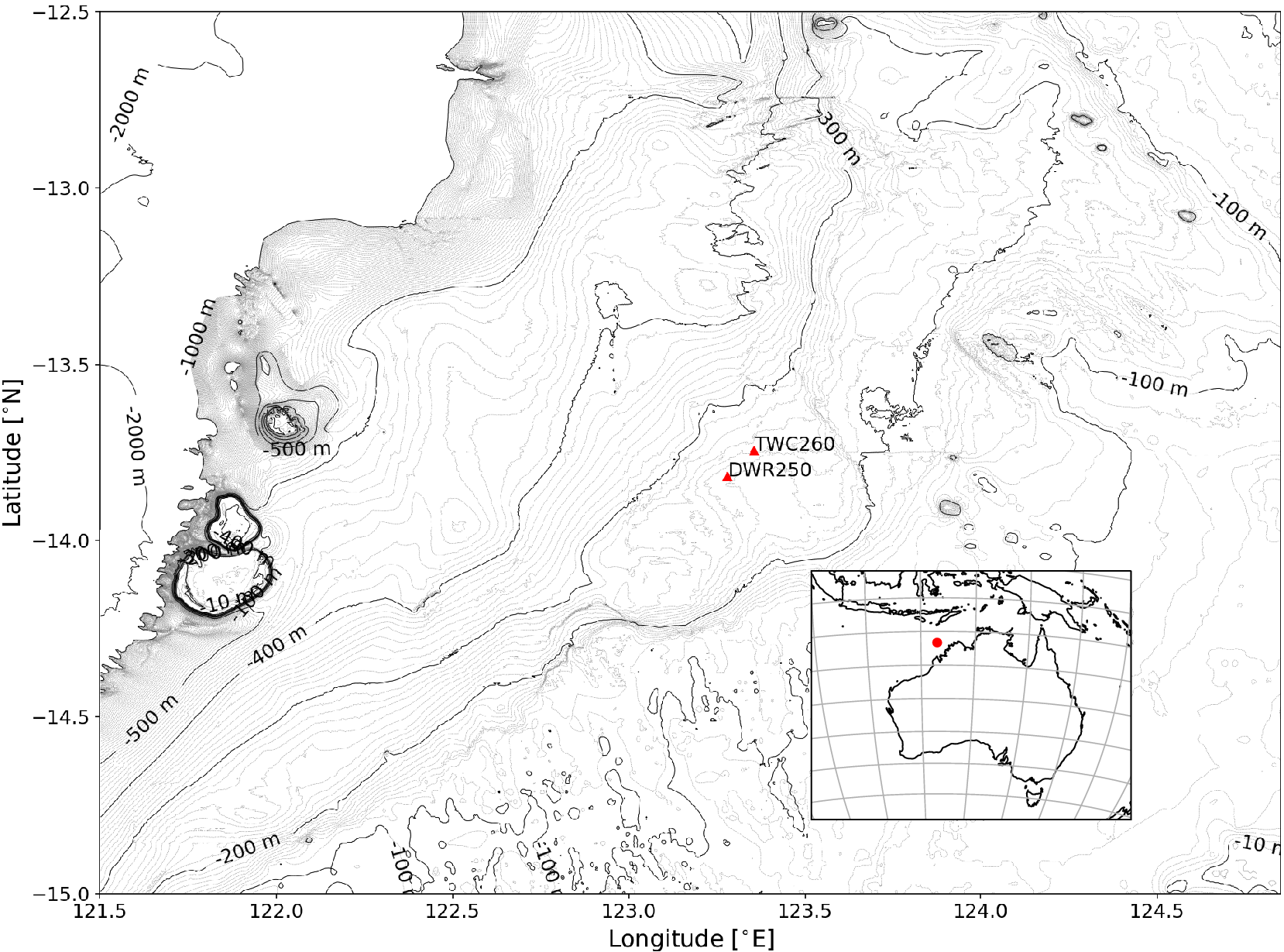
Quantifying uncertainty about surface wind forecasts has a rich history (see, for instance, Cripps et al., Reference Cripps, Nott, Dunsmuir and Wikle2005 and Gneiting et al., Reference Gneiting, Stanberry, Grimit, Held and Johnson2008). This research uses similar data to that in Anderson Loake et al. (Reference Anderson Loake, Astfalck and Cripps2022) and is the next stage in a series of research to quantify uncertainty for NWS operations. Figure 2 shows the location on the NWS that is considered. Data and forecasts are provided in magnitude and direction; however, we translate the polar coordinates into rectangular coordinates so as to ease statistical modeling (see Anderson Loake et al., Reference Anderson Loake, Astfalck and Cripps2022 for full justification of this decision). The scoring rules defined in Section 3 are defined over the wind eastings and northings and so score equivalently over the polar and rectangular coordinates (provided with equivalent statistical inference).
Browse Basin within Australia’s North–West Shelf. Measurements are taken from the site labeled TWC260.
4.1. Measurements
Data are observed hourly from a wind anemometer onboard Prelude FLNG and are typical of the type of measurement device installed at most facilities within the NWS. The dataset spans a 2-year recording period from July 17th, 2017 to July 19th, 2019. We use the period spanning July 17th, 2017 to July 17th, 2018 as training data and the period spanning July 17th, 2018 to July 19th, 2019 as validation data. We show a single week of data with the black line in Figure 3 and a 2D histogram of the entire dataset is in Figure 4. The prevailing seasonal wind pattern is the Indo–Australian monsoon which is predominantly from the South–West in summer months and East in winter months. The wind data exhibit temporal correlation as can be seen in the autocorrelation function (ACF) and partial ACF (pACF) plots in Figure 5. This is in accordance with other statistical research (e.g. Tol, Reference Tol1997; Cripps and Dunsmuir, Reference Cripps and Dunsmuir2003; Anderson Loake et al., Reference Anderson Loake, Astfalck and Cripps2022) where autocorrelation plays a strong role in surface wind modeling. The ACF and pACF plots suggest an approximately 24-hr auto-regressive (AR) order in both the easting and the northing components.
Wind northing and easting measurements from July 4th, 2018 to July 11th, 2018. The red dashed line denotes the time, $ t $
, at which the forecast is made, the thick blue line is the deterministic forecast from the physics-based model, the black solid line shows the observed measurements, and the shaded black line shows the as-of-yet unobserved measurements. This forecast corresponds to the NWP model used in evaluating the scoring rules in Figures 8 and 9.
$ t $
, at which the forecast is made, the thick blue line is the deterministic forecast from the physics-based model, the black solid line shows the observed measurements, and the shaded black line shows the as-of-yet unobserved measurements. This forecast corresponds to the NWP model used in evaluating the scoring rules in Figures 8 and 9.

2D histogram of surface wind easting and northing. The data are of hourly measurements spanning July 17th, 2018 to July 19th, 2019.

ACF and pACF plots of wind easting and northing components.

4.2. Deterministic physics-based forecasting model
We obtain a physics-based numerical model forecast of surface wind from a third-party forecasting contractor. Forecasts are supplied every 6 hr with a minimum prediction horizon of 0 hr (also called “nowcast” values) and maximum prediction horizon of 167 hr. Prediction horizons are supplied hourly from the nowcast value to the 23-hr prediction horizons and then 3 hourly thereafter. A single numerical model forecast is shown in Figure 3. The red dashed line denotes the time when the forecast is made and the blue line is the forecast, in easting and northing components, from the nowcast to the 120-hr prediction horizon (with our defined notation, the red line exists at time $ t $
, and the blue line spans the prediction domain, i.e., the values that
$ t $
, and the blue line spans the prediction domain, i.e., the values that $ h $
may take). The solid black line depicts the observed measurements and the shaded black line represents the as-of-yet unobserved true measurements that the forecasts aim to model. Operational decisions, such as offloading or manoeuvring, require a lead time of up to 48 hr and so we examine the performance of the numerical model (and subsequent probabilistic models that we build) by defining the prediction domain from the nowcast to 48-hr prediction horizons. Physics-based forecasts often have persistent scaling or rotation errors. These errors are seen when coarse numerical models that model atmospheric winds do not downscale wind behavior from the atmosphere to the surface accurately. Incorrect modeling of different wind profiles in different regions can induce scaling errors, and complex surface topographies can cause rotational errors.
$ h $
may take). The solid black line depicts the observed measurements and the shaded black line represents the as-of-yet unobserved true measurements that the forecasts aim to model. Operational decisions, such as offloading or manoeuvring, require a lead time of up to 48 hr and so we examine the performance of the numerical model (and subsequent probabilistic models that we build) by defining the prediction domain from the nowcast to 48-hr prediction horizons. Physics-based forecasts often have persistent scaling or rotation errors. These errors are seen when coarse numerical models that model atmospheric winds do not downscale wind behavior from the atmosphere to the surface accurately. Incorrect modeling of different wind profiles in different regions can induce scaling errors, and complex surface topographies can cause rotational errors.
4.3. Statistical forecasting models
Statistical models of wind prediction broadly fall into two categories: MOS models and time-series models. MOS models are hybrid physics/data models that explicitly utilize the physics-based forecasting model; they aim to correct systematic errors in physics-based forecasting models by regressing the physics-based forecasts onto the observed data (Ranaboldo et al., Reference Ranaboldo, Giebel and Codina2013). They are also used to collate ensembles of numerical forecasts into a single forecasting model (Schuhen et al., Reference Schuhen, Thorarinsdottir and Gneiting2012), and in downscaling coarse global circulation models to regional grid scales (Gonzalez-Aparicio et al., Reference Gonzalez-Aparicio, Monforti, Volker, Zucker, Careri, Huld and Badger2017). The incorporation of probability into MOS models is natural and straightforward; however, not all MOS models are probabilistic, many are fit with appeals to loss function minimization rather that probabilistic approaches (e.g., see Pinson and Hagedorn, Reference Pinson and Hagedorn2012). Herein, we model the bivariate components of the wind so that we account for persistent errors in the numerical models due to scaling and rotation. Time-series models are data-driven models that aim to capture the temporal structure present in the meteorological process. Herein we use a VAR model: a generalization of the AR model to multivariate data. The VAR model captures the relationships of the observed quantities (i.e., wind) as they change through time. Measurements are modeled by regressing the past observations onto the present observations.
The scoring methodology shown applies equally well for comparison of many models but for exposition we consider two models that forecast surface winds. Both models are general in the sense that they do not rely on complex assumptions bespoke to the application and may be straightforwardly implemented for any other asset and location. The first model builds a linear MOS model from the numerical forecasts, and the second builds a time-series model that only requires the observations and not the numerical forecasts. The models are Bayesian, with specification of prior beliefs over all parameters, and inferential procedures to fit each model are available at github.com/TIDE-ITRH/scoringrules. The specifics of the MOS and time-series model specifications are in the Appendix. Both of these models are defined to model the measurements directly (and so incorporate the measurement error in the forecast error). They could be easily extended in a hierarchical framework to incorporate more explicit modeling of measurement error. The forecasting models are purposely built so that one relies on and one is independent of the numerical forecasts so that their value to the operator may be clearly assessed.
4.4. Results
An example of probabilistic forecasts from the MOS model is shown in Figure 6 and from the VAR model in Figure 7—in both these plots the solid blue line denotes the mean forecast and the shaded region denotes the 80% prediction intervals. In Figure 6, for the MOS model, we show the probabilistic forecast out to a 120-hr prediction horizon to demonstrate the advantage that the hybrid physics/data model has in forecasting long lead times. The physics embedded in the model through the numerical forecasts are present in the MOS forecasts, best seen in the Eastings where the large winds between the 8th and 10th of July are accurately predicted. In Figure 7, for the VAR model, we show the probabilistic forecast out to a 48-hr prediction horizon. The VAR model, with its knowledge of the observed data, predicts the first few prediction horizons well and then tends to long-term average wind speed. After 48 hr, the VAR model essentially predicts the long-term wind-speed mean.
Example forecast up to a 120-hr prediction horizon from the fit MOS model. The red dashed line denotes the time at which the forecast has been made, the solid blue line is the mean forecast, the shaded region denotes the 80% prediction interval, the dashed blue line is the forecast from the numerical model, and the black line is the data that are to be observed at the time instance. This forecast corresponds to the MOS model used in evaluating the scoring rules in Figures 8 and 9.

Example forecast up to a 48-hr prediction horizon from from the fit VAR model. The red dashed line denotes the time at which the forecast has been made, the solid blue line is the mean forecast, the shaded region denotes the 80% prediction interval, the dashed blue line is the forecast from the numerical model, and the black line is the data that are to be observed at the time instance. This forecast corresponds to the VAR model used in evaluating the scoring rules in Figures 8 and 9.

For each time $ t $
and prediction horizon
$ t $
and prediction horizon $ h $
, we obtain posterior predictive distributions,
$ h $
, we obtain posterior predictive distributions, $ {F}_{t,h} $
, for both the MOS and VAR models and calculate scores
$ {F}_{t,h} $
, for both the MOS and VAR models and calculate scores $ \mathrm{SE}\left({F}_{t,h},{\mathbf{y}}_{t+h}\right) $
,
$ \mathrm{SE}\left({F}_{t,h},{\mathbf{y}}_{t+h}\right) $
, $ \mathrm{DSS}\left({F}_{t,h},{\mathbf{y}}_{t+h}\right) $
, and
$ \mathrm{DSS}\left({F}_{t,h},{\mathbf{y}}_{t+h}\right) $
, and $ \mathrm{ES}\left({F}_{t,h},{\mathbf{y}}_{t+h}\right) $
as detailed in Section 3. Model skill for the MOS and VAR models is evaluated by averaging the scores at every time instance for each prediction horizon and is shown in Figure 8. The x-axis in Figure 8 represents the model’s skill for each of the future prediction horizons
$ \mathrm{ES}\left({F}_{t,h},{\mathbf{y}}_{t+h}\right) $
as detailed in Section 3. Model skill for the MOS and VAR models is evaluated by averaging the scores at every time instance for each prediction horizon and is shown in Figure 8. The x-axis in Figure 8 represents the model’s skill for each of the future prediction horizons $ h\in \left[0,48\right] $
and so assesses model performance as a function of prediction horizon. We reiterate that it is customary to define scoring rules so that lower scores (and thus lower skill) indicate better performance. By examining all three scores, we can accurately assess the performance of the whole predictive distribution; SE assesses the mean forecast performance, DSS assesses the forecasts tail performance, and ES assesses the body of the forecast. In terms of SE performance, the MOS model is shown to be more accurate than the numerical forecast, indicating a persistent bias in the numerical model. The VAR model is more accurate than the MOS model for the first three prediction horizons and the numerical model for the first four prediction horizons. At the 48-hr prediction horizon, the data-only VAR model is on average approximately
$ h\in \left[0,48\right] $
and so assesses model performance as a function of prediction horizon. We reiterate that it is customary to define scoring rules so that lower scores (and thus lower skill) indicate better performance. By examining all three scores, we can accurately assess the performance of the whole predictive distribution; SE assesses the mean forecast performance, DSS assesses the forecasts tail performance, and ES assesses the body of the forecast. In terms of SE performance, the MOS model is shown to be more accurate than the numerical forecast, indicating a persistent bias in the numerical model. The VAR model is more accurate than the MOS model for the first three prediction horizons and the numerical model for the first four prediction horizons. At the 48-hr prediction horizon, the data-only VAR model is on average approximately $ 1 $
ms
$ 1 $
ms $ {}^{-1} $
worse than the numerical model, which in the order of magnitudes of expected wind behavior at the NWS is not large (see Figure 4). In terms of the ES, again the VAR model scores best for
$ {}^{-1} $
worse than the numerical model, which in the order of magnitudes of expected wind behavior at the NWS is not large (see Figure 4). In terms of the ES, again the VAR model scores best for $ h\le 3 $
, and the MOS model scores best for
$ h\le 3 $
, and the MOS model scores best for $ h>3 $
. For all
$ h>3 $
. For all $ h $
, the VAR model scores better than the numerical forecast model; the difference between this and the SE is that the ES is rewarding the VAR model for quantifying the uncertainty about its forecasts. Finally, the DSS shows similar performance between the MOS and VAR models. Note that the DSS cannot be computed for
$ h $
, the VAR model scores better than the numerical forecast model; the difference between this and the SE is that the ES is rewarding the VAR model for quantifying the uncertainty about its forecasts. Finally, the DSS shows similar performance between the MOS and VAR models. Note that the DSS cannot be computed for $ h=0 $
for the VAR model as the variance of
$ h=0 $
for the VAR model as the variance of $ {F}_{t,0} $
is zero and so the inverse is not defined. The general trend of the scores is similar, indicating that there is no systemic changes in the behavior of the predictive models. Interesting to note that for the ES, the VAR model predicts better than the NWP model over a longer prediction horizon than for the other two scores. This is due to the ES rewarding the uncertainty quantification of the VAR model. The decision to put more or less focus in which score is dependent on the application at hand. For example, critical applications where outliers must be rigorously quantified should focus on DSS, whereas more routine operations that do not need to be risk adverse may be better assessed by SE.
$ {F}_{t,0} $
is zero and so the inverse is not defined. The general trend of the scores is similar, indicating that there is no systemic changes in the behavior of the predictive models. Interesting to note that for the ES, the VAR model predicts better than the NWP model over a longer prediction horizon than for the other two scores. This is due to the ES rewarding the uncertainty quantification of the VAR model. The decision to put more or less focus in which score is dependent on the application at hand. For example, critical applications where outliers must be rigorously quantified should focus on DSS, whereas more routine operations that do not need to be risk adverse may be better assessed by SE.
Calculated scores from the numeric, MOS and VAR models over the 0- to 48-hr prediction horizons. All scores are defined so that lower scores indicate better model performance. For all scores, the VAR model performs best for the first three prediction horizons after which the MOS model performs best. The abbreviation NWP (numerical weather prediction) references the deterministic numeric forecast model.

We may calculate the probabilities of a particular forecasting model scoring best via Monte Carlo (Equation (6))—these probabilities are plotted as a function of prediction horizon in Figure 9. Calculating the probability of best performance is important as it informs the modeler as to the spread of the individual scores (here, the spread of the individual scores indexed by time). Skills are an averaged quantity and so while competing models may have different skill, for any given instance, the variance of the individual scores may dominate the averaged skill. Definitive results as to the performance of competing models require (1) a lower skill (i.e., better performance on average) and (2) a high probability of best performance (i.e., how often does a particular model perform best).
Probability of best score from the numeric, MOS and VAR models over the 0- to 48-hr prediction horizons. For all scores, the VAR model has the highest probability of scoring best for the first three prediction horizons after which the MOS model performs best. The abbreviation NWP (numerical weather prediction) references the deterministic numeric forecast model.

Reflecting what is seen in horizon scores in Figure 8, the VAR model performs best for the first three prediction horizons, and the MOS model performs best thereafter. The MOS model shows a much larger probability of scoring better than the numerical model for the DSS and ES and roughly equal probability for SE. This indicates that the improved mean SE score in Figure 8 is largely dwarfed by the predictive variability (as there is separation of the means, but not so clear separation of the predictive process), but for the other scores there is a clear advantage to quantifying the error process.
5. Discussion and Concluding Remarks
The results shown in the case study provide objective measures by which the operator may judge forecasting models. We define scoring rules that evaluate the entire forecast distribution and further provide a clear framework by which future forecasting products may be judged. We argue that forecasting model performance may be sufficiently captured by three scoring rules: SE, a measure of the mean discrepancy of the forecast; the DSS, a measure of a forecasts ability to model tail events; and the ES, a measure of a forecasts ability to model the center of the distribution. By defining the scores as, in the case study herein, a function of the prediction horizon, and more broadly as a function of some prediction domain, decisions as to what forecasting model to adopt depending on what operation it is informing can be made. By examining a suite of scoring rules, we provide confidence in a models ability to predict both the mean process (via SE) and the forecast uncertainty (via the DSS and ES). Further, assessing model performance as a function of prediction horizon allows us to judge what forecasting model is best for different purposes.
The case study used herein is a real dataset provided by an offshore operator. The examples of the statistical models developed herein are viewed by the authors as being the bare minimum comparison against which the value of a numerical forecast should be assessed. Modeling winds is vital to maritime activity, and the demand to understand wind behavior at different horizons is increasing with new and nascent offshore wind developments. Predictions that affect long-term decisions such as design, where nonreal-time data, such as site characterizations, are used; medium-term decisions such as vessel offloading; and short-term decisions such as those due to immediate energy demands need to be evaluated with these goals in mind. Evaluating competing predictive models and the value of measured data can help to justify the associated costs. For instance, are the costs of a state-of-the-art numerical forecasting service or monitoring system worthwhile, or would a cheaper solution be sufficient.
With the increasing development of probabilistic forecasting models for maritime operations, we hope so too comes the adoption of appropriate validation procedures. As this special edition of Data-Centric Engineering shows, there is an increasing appetite for statistical advances within maritime engineering. We present methodology by which statistical forecasting models may be judged transparently and with rigor.
Acknowledgments
We thank the reviewers who provided insightful comments and edits. Their contribution has made this a better and more approachable body of work.
Author contribution
All authors contributed to the conceptualization, research, and writing of this manuscript. L.A. curated the data and performed the analysis for the case study. E.C. supervised the project.
Competing interest
The authors declare none.
Data availability statement
Code is available at github.com/TIDE-ITRH/scoringrules. Anonymized data have been provided and should only be counted as representative data used to execute the code. Results presented herein are generated with the original data that are not made available publicly due to confidentiality.
Funding statement
All authors are supported by the ARC ITRH for Transforming energy Infrastructure through Digital Engineering (TIDE, http://TIDE.edu.au) which is led by The University of Western Australia, delivered with The University of Wollongong and several other Australian and International research partners, and funded by the Australian Research Council, INPEX Operations Australia, Shell Australia, Woodside Energy, Fugro Australia Marine, Wood Group Kenny Australia, RPS Group, Bureau Veritas and Lloyd’s Register Global Technology (Grant No. IH200100009). Michael Bertolacci was further supported by the Australian Research Council (ARC) Discovery Project (DP) DP190100180.
A. Model Specifications
A.1. Model 1: Model Output Statistics
Define $ {\mathbf{y}}_t $
as the observed vector of wind speed at time
$ {\mathbf{y}}_t $
as the observed vector of wind speed at time $ t $
and
$ t $
and $ {\mathbf{f}}_{t,h} $
as the deterministic numerical forecast made at time
$ {\mathbf{f}}_{t,h} $
as the deterministic numerical forecast made at time $ t $
for time
$ t $
for time $ t+h $
(and so
$ t+h $
(and so $ {\mathbf{f}}_{t,h} $
is the forecast of the
$ {\mathbf{f}}_{t,h} $
is the forecast of the $ h $
hour prediction horizon at time
$ h $
hour prediction horizon at time $ t $
). We model
$ t $
). We model
 $$ {\mathbf{y}}_{t+h}={\beta}_{0,h}+{\boldsymbol{\beta}}_{1,h}{\mathbf{f}}_{t,h}+{\boldsymbol{\beta}}_{2,h}{\mathbf{f}}_{t-6,h+6}+{\varepsilon}_{t,h} $$
for all $ h\in \Omega $
, where
$ h\in \Omega $
, where $ {\beta}_{0,h} $
is a
$ {\beta}_{0,h} $
is a $ 2\times 1 $
intercept term,
$ 2\times 1 $
intercept term, $ {\boldsymbol{\beta}}_{1,h} $
and
$ {\boldsymbol{\beta}}_{1,h} $
and $ {\boldsymbol{\beta}}_{2,h} $
are
$ {\boldsymbol{\beta}}_{2,h} $
are $ 2\times 2 $
scaling matrices, and
$ 2\times 2 $
scaling matrices, and $ {\varepsilon}_{t,h}\sim \mathcal{N}\left(0,{\Sigma}_h\right) $
is a
$ {\varepsilon}_{t,h}\sim \mathcal{N}\left(0,{\Sigma}_h\right) $
is a $ 2\times 1 $
dimensional residual with variance
$ 2\times 1 $
dimensional residual with variance $ {\Sigma}_h $
. Parameters
$ {\Sigma}_h $
. Parameters $ {\beta}_{0,h} $
,
$ {\beta}_{0,h} $
, $ {\boldsymbol{\beta}}_{1,h} $
,
$ {\boldsymbol{\beta}}_{1,h} $
, $ {\boldsymbol{\beta}}_{2,h} $
, and
$ {\boldsymbol{\beta}}_{2,h} $
, and $ {\Sigma}_h $
are all specific to a horizon
$ {\Sigma}_h $
are all specific to a horizon $ h $
. The term
$ h $
. The term $ {\mathbf{f}}_{t-6,h+6} $
is the previous forecast for time
$ {\mathbf{f}}_{t-6,h+6} $
is the previous forecast for time $ t+h $
, this term is sometimes found to be more accurate than
$ t+h $
, this term is sometimes found to be more accurate than $ {\mathbf{f}}_{t,h} $
due to model spin-up when the internal conditions of the model are not dynamically balanced (e.g., see Kleczek et al., Reference Kleczek, Steeneveld and Holtslag2014). Each forecast
$ {\mathbf{f}}_{t,h} $
due to model spin-up when the internal conditions of the model are not dynamically balanced (e.g., see Kleczek et al., Reference Kleczek, Steeneveld and Holtslag2014). Each forecast $ {\mathbf{f}}_{t,h} $
attempts to model the random variable
$ {\mathbf{f}}_{t,h} $
attempts to model the random variable $ {\mathbf{Y}}_{t,h} $
of which
$ {\mathbf{Y}}_{t,h} $
of which $ {\mathbf{y}}_{t+h} $
is the observed value. Random variables
$ {\mathbf{y}}_{t+h} $
is the observed value. Random variables $ {\mathbf{Y}}_{t-h,h} $
for
$ {\mathbf{Y}}_{t-h,h} $
for $ h\in \Omega $
model the same point in time
$ h\in \Omega $
model the same point in time $ t $
with observation
$ t $
with observation $ {\mathbf{y}}_t $
; the
$ {\mathbf{y}}_t $
; the $ {\mathbf{Y}}_{t-h,h} $
differ in that they are with respect to different information sets, that is, we have different information for different
$ {\mathbf{Y}}_{t-h,h} $
differ in that they are with respect to different information sets, that is, we have different information for different $ h $
. The model is Bayesian and prior distributions are specified as
$ h $
. The model is Bayesian and prior distributions are specified as $ {\beta}_{0,h}\sim \mathcal{N}\left(0,\mathbf{I}\right) $
,
$ {\beta}_{0,h}\sim \mathcal{N}\left(0,\mathbf{I}\right) $
, $ {\boldsymbol{\beta}}_{1,h}\sim \mathrm{\mathcal{M}}\mathcal{N}\left(\mathbf{I},\mathbf{I},\mathbf{I}\right) $
,
$ {\boldsymbol{\beta}}_{1,h}\sim \mathrm{\mathcal{M}}\mathcal{N}\left(\mathbf{I},\mathbf{I},\mathbf{I}\right) $
, $ {\boldsymbol{\beta}}_{2,h}\sim \mathrm{\mathcal{M}}\mathcal{N}\left(0,\mathbf{I},\mathbf{I}\right) $
, and
$ {\boldsymbol{\beta}}_{2,h}\sim \mathrm{\mathcal{M}}\mathcal{N}\left(0,\mathbf{I},\mathbf{I}\right) $
, and $ {\Sigma}_h\sim \mathrm{\mathcal{I}}\mathcal{W}\left(\mathrm{2,0.05}\ast \mathbf{I}\right) $
where
$ {\Sigma}_h\sim \mathrm{\mathcal{I}}\mathcal{W}\left(\mathrm{2,0.05}\ast \mathbf{I}\right) $
where $ \mathbf{I} $
is a
$ \mathbf{I} $
is a $ 2\times 2 $
identify matrix,
$ 2\times 2 $
identify matrix, $ \mathcal{N}\left(\cdot, \cdot \right) $
denotes the normal distribution,
$ \mathcal{N}\left(\cdot, \cdot \right) $
denotes the normal distribution, $ \mathrm{\mathcal{M}}\mathcal{N}\left(\cdot, \cdot, \cdot \right) $
the matrix-normal distribution, and
$ \mathrm{\mathcal{M}}\mathcal{N}\left(\cdot, \cdot, \cdot \right) $
the matrix-normal distribution, and $ \mathrm{\mathcal{I}}\mathcal{W}\left(\cdot, \cdot \right) $
the inverse-Wishart distribution.
$ \mathrm{\mathcal{I}}\mathcal{W}\left(\cdot, \cdot \right) $
the inverse-Wishart distribution.
A.2. Model 2: Vector Auto-Regressive Modeling
We build a VAR model based only on the observed wind measurements. VAR processes with long correlation lengths are prone to overfitting as the number of parameters grows quadratically with the dimension of the process and linearly with $ p $
(Jochmann et al., Reference Jochmann, Koop and Strachan2010). We use a stochastic selection representation of the VAR process, developed by Korobilis (Reference Korobilis2013), to promote model parsimony and prevent such issues. Each observation
$ p $
(Jochmann et al., Reference Jochmann, Koop and Strachan2010). We use a stochastic selection representation of the VAR process, developed by Korobilis (Reference Korobilis2013), to promote model parsimony and prevent such issues. Each observation $ {\mathbf{y}}_t $
is modeled as
$ {\mathbf{y}}_t $
is modeled as
 $$ {\mathbf{y}}_t=\mu +\sum \limits_{i=1}^p\left({\Gamma}_i\odot {\Phi}_i\right)\left({\mathbf{y}}_{t-i}-\mu \right)+{\varepsilon}_t $$
where $ \mu $
is a
$ \mu $
is a $ 2\times 1 $
mean constant over time,
$ 2\times 1 $
mean constant over time, $ p $
is the order of the VAR process,
$ p $
is the order of the VAR process, $ {\Phi}_i $
is the
$ {\Phi}_i $
is the $ i $
th
$ i $
th $ 2\times 2 $
lag matrix, the
$ 2\times 2 $
lag matrix, the $ {\Gamma}_i $
are
$ {\Gamma}_i $
are $ 2\times 2 $
stochastic selection matrices with elements either
$ 2\times 2 $
stochastic selection matrices with elements either $ 0 $
or
$ 0 $
or $ 1 $
, and
$ 1 $
, and $ {\varepsilon}_t $
is the
$ {\varepsilon}_t $
is the $ 2\times 1 $
residual distributed
$ 2\times 1 $
residual distributed $ {\varepsilon}_t\sim \mathcal{N}\left(0,\Sigma \right) $
. The operator
$ {\varepsilon}_t\sim \mathcal{N}\left(0,\Sigma \right) $
. The operator $ \odot $
denotes element-wise multiplication so that matrix
$ \odot $
denotes element-wise multiplication so that matrix $ {\Gamma}_i $
controls the number of nonzero elements in
$ {\Gamma}_i $
controls the number of nonzero elements in $ \left({\Gamma}_i\odot {\Phi}_i\right) $
. Forecasts from the VAR model are described via the forward propagation of the auto-regressive structure. We specify prior distributions
$ \left({\Gamma}_i\odot {\Phi}_i\right) $
. Forecasts from the VAR model are described via the forward propagation of the auto-regressive structure. We specify prior distributions $ \mu \sim \mathcal{N}\left(0,\mathbf{I}\right) $
,
$ \mu \sim \mathcal{N}\left(0,\mathbf{I}\right) $
, $ {\Phi}_1\sim \mathrm{\mathcal{M}}\mathcal{N}\left(0.9\mathbf{I},\mathbf{I},\mathbf{I}\right) $
,
$ {\Phi}_1\sim \mathrm{\mathcal{M}}\mathcal{N}\left(0.9\mathbf{I},\mathbf{I},\mathbf{I}\right) $
, $ {\Phi}_i\sim \mathrm{\mathcal{M}}\mathcal{N}\left(0,\mathbf{I},\mathbf{I}\right) $
for
$ {\Phi}_i\sim \mathrm{\mathcal{M}}\mathcal{N}\left(0,\mathbf{I},\mathbf{I}\right) $
for $ i\in \left\{2,\dots, p\right\} $
, and
$ i\in \left\{2,\dots, p\right\} $
, and $ \Sigma \sim \mathrm{\mathcal{I}}\mathcal{W}\left(\mathrm{2,0.05}\ast \mathbf{I}\right) $
. Each element of the
$ \Sigma \sim \mathrm{\mathcal{I}}\mathcal{W}\left(\mathrm{2,0.05}\ast \mathbf{I}\right) $
. Each element of the $ {\Gamma}_{i\left[a,b\right]} $
is modeled independently as a Bernoulli random variable
$ {\Gamma}_{i\left[a,b\right]} $
is modeled independently as a Bernoulli random variable $ {\left({\Gamma}_i\right)}_{\left[a,b\right]}\sim \mathrm{\mathcal{B}}(0.5) $
. We choose
$ {\left({\Gamma}_i\right)}_{\left[a,b\right]}\sim \mathrm{\mathcal{B}}(0.5) $
. We choose $ p=24 $
as the pACF plots in Figure 5 suggest 24 hr of temporal correlation—this too is seen in Anderson Loake et al. (Reference Anderson Loake, Astfalck and Cripps2022).
$ p=24 $
as the pACF plots in Figure 5 suggest 24 hr of temporal correlation—this too is seen in Anderson Loake et al. (Reference Anderson Loake, Astfalck and Cripps2022).


 Open access
Comments
No Comments have been published for this article.