


1. Introduction
The Murchison Widefield Array (MWA; Tingay et al. Reference Tingay2013) is a low frequency aperture array (LFAA) radio interferometer, and is a precursor to the Square Kilometre Array LFAA (SKA-Low). The MWA is comprised of 256 tile stations, 128 of which can operate at any one time. Each tile is a collection of 16 dual-polarised dipoles arranged in a  $4\times4$ North-South, East-West grid. These tiles are capable of observing in the frequency range of
  $70-320\,\textrm{MHz}$, with an instantaneous bandwidth of
 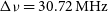 $\Delta\nu = 30.72\,\textrm{MHz}$. Each observing band is comprised of 24 coarse channels with 1.28 MHz bandwidth. The number and layout of the MWA tiles provides an excellent snapshot uv-coverage, in conjunction with the typical widefield of view for LFAAs, the MWA is well suited to quickly surveying the entire sky (Tingay et al. Reference Tingay2013; Ord et al. Reference Ord2015; Wayth et al. Reference Wayth2018). As part of the Galactic and extra-galactic all-sky MWA survey (GLEAM; Wayth et al. Reference Wayth2015), the MWA observed the entire radio sky south of declination (DEC)
  $+25^{\circ}$ in the frequency range
  $72-231\,\textrm{MHz}$. The MWA additionally observed the entire sky at 300 MHz during an extended observing run in the second year of the GLEAM survey.
Orthographic projection of the Stokes I MWA  $300\,\textrm{MHz}$ FEE beam model (Sokolowski et al. Reference Sokolowski2017), generated at
  $\phi=0^{\circ}$, and
  $\theta_\textrm{zen} = 0^{\circ},30^{\circ},45^{\circ}$. The centre of the main lobe is marked with a solid red circle, the approximate grating lobe centres are marked with sold red crosses, and the most prominent grating lobe centre is marked with a solid red triangle. The solid black contours show the beam response at levels of
  $10^{-3},10^{-2},10^{-1}$ and
  $0.9$ of the maximum and match the black lines in the colourbars. The dashed black lines are constant zenith lines. This series of subfigures shows how the MWA FEE beam model changes with pointing along one axis (the zenith axis). Due to the symmetry of the array this also describes the East-West as well as North-South primary beam configuration.
Unlike dish arrays the MWA electronically points by introducing a delay in the signal between each dipole in a tile. The tile then combines each dipole to form a beam response pattern on the sky (the primary beam) (Ord et al. Reference Ord2010). For most of the MWA frequency range the primary beam is dominated by the main lobe which is aligned with the pointing direction. However, at high frequencies when the dipole separation is comparable to the observing wavelength, highly sensitive sidelobes known as grating lobes appear in the primary beam pattern. These grating lobes are reflections of the main lobe and appear above the horizon at a frequency around  ${\sim}300$ MHz for the MWA (Sutinjo et al. Reference Sutinjo, O’Sullivan, Lenc, Wayth, Padhi, Hall and Tingay2015). For a zenith pointed observation the MWA primary beam at
  $300\,\textrm{MHz}$ is composed of the main lobe positioned at zenith, and four grating lobes located
  ${\sim}51^{\circ}$ North, South, East and West relative to the main lobe, this can be seen in Subfigure 1a where the main lobe and the grating lobes are identified by the red markers. At this projection these grating lobes are
  ${\sim}40\%$ as sensitive as the main lobe (see the contours in Subfigure 1a). With a pointing away from zenith, the primary beam projection changes, this affects the size and relative sensitivity of the grating lobes, but not the relative position of the grating lobes with respect to the main lobe. In Subfigure 1b and 1c we show two example primary beam patterns with a pointing centre zenith (
 $\theta_\textrm{zen}$) angle of
  $60^{\circ}$ in Figure 1b and a pointing angle of
  $\theta_\textrm{zen} = 45^{\circ}$ in Subfigure 1c, both with an azimuth (
 $\phi$) angle of
  $0^{\circ}$. These two subfigures show how the primary beam pattern evolves as the pointing direction approaches the horizon. As the main lobe moves northward, the northern grating lobe disappears effectively below the horizon and the southern grating lobe increases in prominence. The peak sensitivity of the southern grating lobe approaches that of the main lobe becoming the most prominent grating lobe. Correspondingly the primary beam pattern towards the southern horizon loses overall sensitivity. Due to the symmetry of the primary beam pattern from the regular grid dipole layout, this behaviour is replicated when the main lobe is oriented towards the South, East and West. Diagonal pointings have the same effect, where a North-East pointing will result in an increase in prominence of the South and West grating lobes.
In the high frequency MWA regime ( $\nu \gtrsim 280\,\textrm{MHz}$), the combined sensitivity of the grating lobes can detect more radio emission than the main lobe of the primary beam; contrary to the low frequency MWA primary beam. Bright sources present in these grating lobes introduce point spread function (PSF) sidelobe structures that affect the sensitivity of the main lobe. The higher frequency regime is also heavily affected by radio-frequency interference (RFI), where the coarse channels around
  $280\,$MHz, have high mean RFI occupancy rates of
  ${\sim}$20–80%. See Figure 3 of Sokolowski, Wayth, & Lewis (Reference Sokolowski, Wayth and Lewis2015) for further details. As a result of RFI, instrumental limitations, and the presence of grating lobes, observations are typically limited to the 70–230 MHz frequency range. These issues make calibrating and imaging 300 MHz MWA observations more complex than at lower frequencies, and until now the high frequency regime has largely been neglected.
There are however potential benefits to observing at 300 MHz with the MWA. At 300 MHz the Phase II MWA extended configuration (Wayth et al. Reference Wayth2018) has a resolution comparable to the  $45\,\textrm{arcsec}$ resolution of the 1.4 GHz NRAO VLA Sky Survey (NVSS; Condon et al. Reference Condon, Cotton, Greisen, Yin, Perley, Taylor and Broderick1998). This allows for a direct comparison between dish arrays and LFAAs, leading to a better understanding of the systematic differences between the different kinds of radio interferometers. Observations at 300 MHz will also further constrain the spectral energy densities (SEDs) of radio sources; along with the higher resolution at 300 MHz which will aid in the classification of radio sources. Sources with spectral peaks at
  $\nu \geq 300\,\textrm{MHz}$ may be too faint to be detected at lower frequencies. The MWA may be more sensitive to some of these peak spectrum sources at 300 MHz, due to relative positive spectral indices of sources within the MWA frequency rangeFootnote a. Due to the squared wavelength
  $(\lambda^2)$ dependence of Faraday rotation, polarised radio sources at higher MWA frequencies are significantly less depolarised than sources at lower MWA frequencies (Farnsworth et al. Reference Farnsworth, Rudnick and Brown2011). Grating lobes also pose a problem for polarisation studies, therefore a calibration method for 300 MHz observations could open the door to more sensitive MWA polarisation observations. Calibrated 300 MHz polarisation observations could add high value to existing low frequency polarisation work (Lenc et al. Reference Lenc2017; Riseley et al. Reference Riseley2018; Reference Riseley2020).
In this work we describe a 300 MHz sky-model catalogue which is constructed from cross-matched low and high frequency catalogues. In particular this work uses GLEAM and NVSS to interpolate the sky flux density at 300 MHz. We also use the fully embedded element (FEE; Sokolowski et al. Reference Sokolowski2017) MWA tile beam model. The FEE MWA tile beam models each coarse channel in the frequency range 72–315 MHz. Using the FEE beam model in conjunction with the 300 MHz sky-model, we can calibrate MWA observations using the sky-model calibration method. In particular we use the direction independent calibration software calibrate (Offringa et al. Reference Offringa2016). calibrate is based on the direction independent part of the Mitchcal algorithm (Mitchell et al. Reference Mitchell, Greenhill, Wayth, Sault, Lonsdale, Cappallo, Morales and Ord2008), which uses an apparent sky-model generated by the MWA tile beam and a sky catalogue to calibrate the gain amplitude and phases for each tile. In this work we use calibrate to process a calibrator 300 MHz MWA observation. The calibration solutions from this observation can then be transferred to another observation at the same pointing taken on the same observing night.
This paper is divided into the following sections: Section 2 discusses the low and high frequency catalogues that are interpolated to create the 300 MHz sky-model; Section 3 details the sky-model, and the SED fitting processes; Section 4 introduces the observations used to demonstrate the calibration and imaging strategy used in this work; Section 5 discusses the calibration strategy; Section 6 discusses the imaging strategy; Section 7 introduces the images produced from the test observations; Section 8 discusses the results and concludes the work.
2. Low & high frequency catalogues
In this section we describe the low and high frequency catalogues that cover the sky below  $\textrm{DEC} \leq +45^{\circ}$, in the frequency range 72 to
  $1.4\,\rm{GHz}$. The majority of the sky is covered by the GLEAM extra-galactic catalogue (GLEAM_exGal; Hurley-Walker et al. Reference Hurley-Walker2017). This catalogue forms the basis for the 300 MHz sky-model discussed further in (Section 3). GLEAM_exGal is missing several regions, particularly around the Galactic plane (GP), the large and small Magellanic clouds (LMC, SMC), around Centaurus A (CenA), and in two wedge shaped regions. GLEAM_exGal is also missing a set of exceptionally bright calibrator radio sources, as well regions above
  $\textrm{DEC} \geq +30^{\circ}$ (Hurley-Walker et al. Reference Hurley-Walker2017). These missing regions can be filled in with later releases of the GLEAM data (For et al. Reference For2018; Hurley-Walker et al. Reference Hurley-Walker2019b), as well as from other high and low frequency surveys at higher declinations such as NVSS and the TIFR Giant Metrewave Radio Telescope
  $150\,\rm{MHz}$ all-sky radio survey ADR1 (TGSS; Intema et al. Reference Intema, Jagannathan, Mooley and Frail2017). These surveys are discussed in Sections 2.2 and 2.3. Additionally we describe several bespoke source models which were created from existing GLEAM images, and supplemented with high accuracy SED models from Perley & Butler (Reference Perley and Butler2017). These source models are critical for calibration purposes and are discussed in Section 2.4.
2.1. PUMA catalogue
Properly cross-matching catalogues with different sensitivities and resolutions is complex, therefore we use the Positional Update and Matching Algorithm (Line et al. Reference Line, Webster, Pindor, Mitchell and Trott2017, PUMA). We use a PUMA-created catalogue which combines the GLEAM_exGal catalogue with higher frequency catalogues (J. Line, personal communications). We hereon refer to the PUMA catalogue as PUMAcat. PUMAcat was created by cross-matching the GLEAM_exGal catalogue with the following surveys: the 74 MHz Very Large Array Low Frequency Sky Survey redux (VLSSr; Lane et al. Reference Lane, Cotton, van Velzen, Clarke, Kassim, Helmboldt, Lazio and Cohen2014), TGSS (Intema et al. Reference Intema, Jagannathan, Mooley and Frail2017), the 843 MHz Sydney University Molonglo Sky Survey (SUMSS; Bock, Large, & Sadler (Reference Bock, Large and Sadler1999), NVSS (Condon et al. Reference Condon, Cotton, Greisen, Yin, Perley, Taylor and Broderick1998).
PUMAcat contains  $308\,584$ radio sources and covers a frequency range of
  $72\,\rm{MHz}$ to
  $1.4\,\rm{GHz}$, including (where possible) the full GLEAM bands from
  $72\,\rm{MHz}$ to
  $231\,\rm{MHz}$. Table 1 breaks down the different source types in PUMAcat. The sources classified isolated, multiple, and dominant in Table 1 are defined in Line et al. (Reference Line, Webster, Pindor, Mitchell and Trott2017). The
  $5\,203$ sources defined as N/A are GLEAM_exGal sources which did not have any corresponding matches in the other catalogues. The 783 Aegean sources are a bespoke extended source model developed by Line et al. (Reference Line, Webster, Pindor, Mitchell and Trott2017) for the EoR0Footnote b field.
Break down of the different match type sources in PUMAcat.
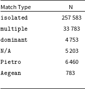
The last class of sources are the  $6\,460$ Pietro sources from Procopio et al. (Reference Procopio2017) which were derived from a deep 6 h MWA survey of the EoR1Footnote c field in the 182 MHz band. In PUMAcat these sources have their own spectral values for the frequencies 170 , 190 and 210 MHz. These values come from fitting across the 182 MHz band with a second order polylogarithmic function. In Procopio et al. (Reference Procopio2017) this was done to ensure smooth spectral behaviour when calibrating their observations. The flux density errors for the fitted bands were not recorded and as a result these sources do not have any quoted errors in PUMAcat. To estimate the error in the Pietro bands we calculated the median relative error for each of the GLEAM subbands in PUMAcat. We then fit the relative error in the subbands with a second order polynomial. Using the second order fit we estimated the relative error in each of the fitted Pietro bands and updated PUMAcat. We additionally filtered 20 sources from PUMAcat which either had one or no flux density measurements.
2.2. GLEAM supplementary sky-model
The aforementioned missing regions in GLEAM_exGal can be filled in using the GLEAM 200 MHz sky-model created to calibrate MWA Phase II data. This sky-model is constructed from processed publicly available GLEAM data (Wayth et al. Reference Wayth2015). Specifically it includes missing regions from recent publications (For et al. Reference For2018; Hurley-Walker et al. Reference Hurley-Walker2019b), and unpublished processed public GLEAM data around CenA (Hurley-Walker et al. Reference Hurley-Walker, Hancock, Anderson, Morgan, Duchesne and Galvin2019a). The main purpose of this GLEAM sky-model is to process the GLEAM extended survey (GLEAM-X) data (Hurley-Walker et al. in prep). This model is publicly available through the GLEAM-XFootnote d GitHub repository (Hurley-Walker et al. Reference Hurley-Walker, Hancock, Anderson, Morgan, Duchesne and Galvin2019a). The GLEAM sky-model additionally contains multi-component source models for Hydra A and Virgo A, these will be further discussed in Section 2.4.
For the purposes of this work we only require a subset of the GLEAM sky-model which covers the missing regions in PUMAcat. We cross-matched the GLEAM sky-model to PUMAcat at a separation of 2 arcminutes. The GLEAM sky-model sources that did not have matches with PUMAcat were formed into a subset catalogue. Excluding the two wedge regions, this subset catalogue contains  $48\,816$ sources which cover the missing GP, LMC, SMC and CenA regions in GLEAM_exGal. This subset catalogue is hereon referred to as the GLEAM supplementary catalogue (GLEAM_Sup).
2.3. TGSS/NVSS spectral index catalogue
The remaining missing regions from GLEAM_exGal which needFootnote e to be filled in are the two wedge regions, and declinations higher than  $+30^{\circ}$. For the observations considered in this work and Cook (Reference Cook2020) we only considered a modest declination increase up to
  $+45^{\circ}$. This was sufficient to test the calibration strategy for these observation, because strong sources such as Cygnus A, and Cassiopeia A (for example) were below the horizon. However, in future work it may be necessary to include these bright sources and others to the total sky-model, to be able to calibrate observations collected at any LST.
To cover these missing regions and higher declinations we use the TGSS/NVSS spectral index catalogue, where de Gasperin, Intema, & Frail (Reference de Gasperin, Intema and Frail2018) cross-matched the first TGSS (Intema et al. Reference Intema, Jagannathan, Mooley and Frail2017) data release with NVSS (Condon et al. Reference Condon, Cotton, Greisen, Yin, Perley, Taylor and Broderick1998). This catalogue covers the frequency range  $150\,\rm{MHz}$ to
  $1.4\,\rm{GHz}$, and the entire sky above declination
  $-40^{\circ}$. Importantly this work investigated the spectral index
  $\alpha^{150}_{1\,400}$ of these sources. This is useful because it allows for the interpolation of the 300 MHz flux density. Interpolation will be discussed further in Section 3.3.
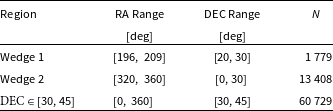
In this work we took only the single (S), multiple (M) and Complex (C) sources from the catalogue (for a definition of these sources see de Gasperin et al. (Reference de Gasperin, Intema and Frail2018)). Sources with only a single detection in either NVSS or TGSS were ignored since the sensitivity of both of these surveys is deeper than the GLEAM survey. Additionally sources identified as island (I) were internally cross-matched to removed double detections. These are hold overs from the cross-matching method used by de Gasperin et al. (Reference de Gasperin, Intema and Frail2018) to join the two catalogues. After the filtering process the total number of sources for each of the three subset regions is given in Table 2.
The final number of sources in the two wedge regions, and the declination strip from  $+30^{\circ} < \textrm{DEC} \leq +45^{\circ}$.
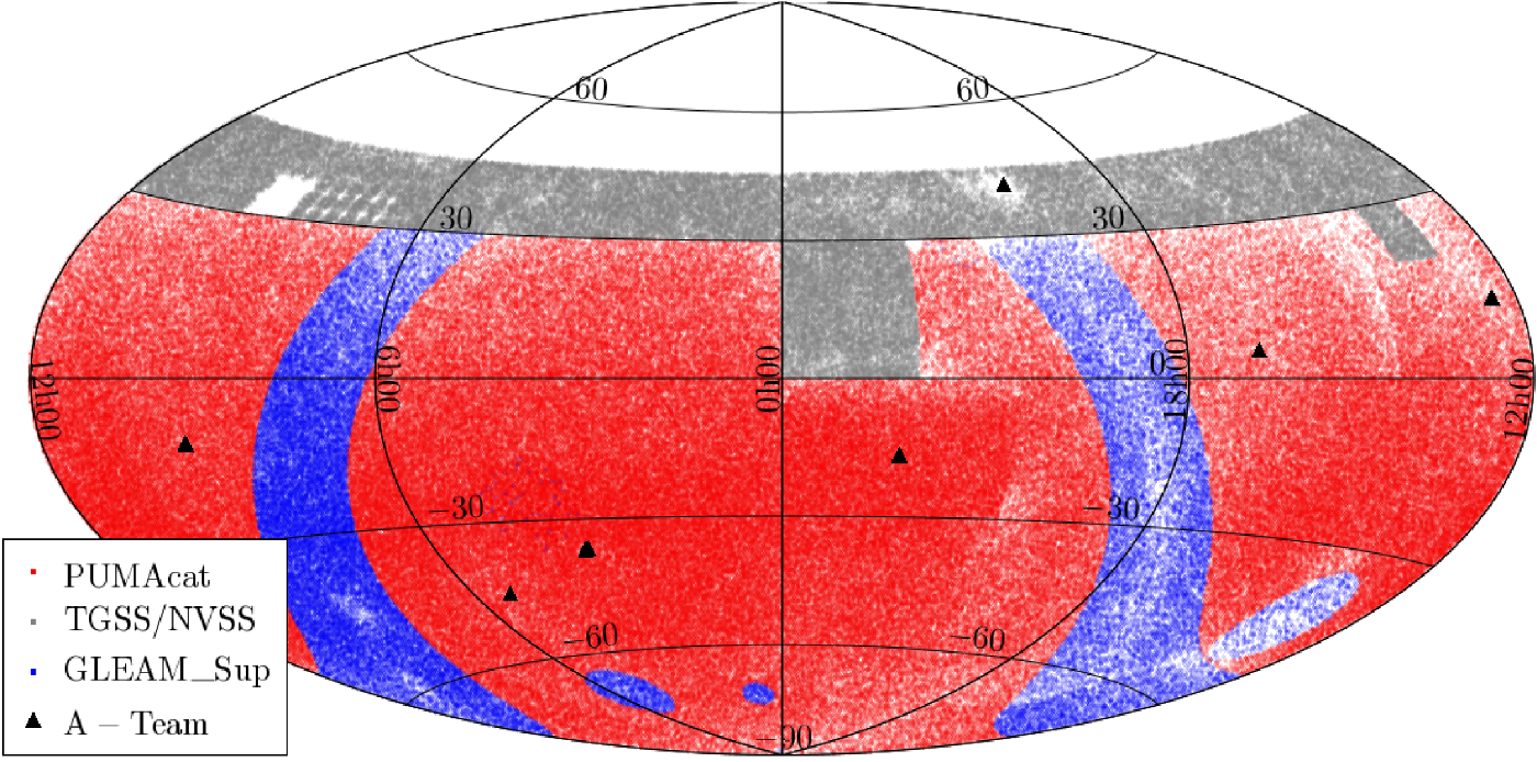
Aitoff projection showing the sky coverage of PUMAcat (red), TGSS/NVSS (light grey) subset and the GLEAM_Sup catalogue (blue). The black triangles indicate the position of A-team sources. Gaps are present in the TGSS/NVSS catalogue at  $97^{\circ}.5 \leq \textrm{RA} \leq 142^{\circ}.5$ and DEC range
  $25^{\circ}\leq \textrm{DEC} \leq 39^{\circ}$, these gaps are a result of missing data in the TGSS catalogue (Intema et al. Reference Intema, Jagannathan, Mooley and Frail2017). Additional gaps occur at the boundary between the TGSS/NVSS catalogue, and the other catalogues.
2.4. Bright calibrator sources
The calibrator sources are a set of exceptionally bright radio galaxies which are not present in GLEAM_exGal (Hurley-Walker et al. Reference Hurley-Walker2017). Some of these sources are arcminutes to degrees in size (Pictor A, Fornax A, and Centaurus A for example), others such as 3C444 are not fully resolved at lower MWA frequencies, but are potentially resolved at 300 MHz. Due to the magnitude of their brightness these sources are often used as calibrators for interferometric radio observations. As such accurate SEDs and spatial models for these sources are necessary for creating accurate calibration solutions for 300 MHz MWA observations.
Some multi-component Gaussian models exist in the GLEAM sky-model for Hydra A and Virgo A. For the remaining calibrator sources we created bespoke point source models for Pictor A, 3C444, Cygnus A, Hercules A and Fornax A using cutout GLEAM imagesFootnote f (Wayth et al. Reference Wayth2015). The highest resolution 227 MHz GLEAM band cutout images for these sources were used. For the unresolved sources only a single point source model was fit. For partially resolved sources we used NVSS cutout imagesFootnote g, and fit two point sources since these sources might be resolved at 300 MHz (Condon et al. Reference Condon, Cotton, Greisen, Yin, Perley, Taylor and Broderick1998). Spatially resolved complex sources such as Fornax A required more attention. We fit 18 point sources to Fornax A, one to the core, and 17 to the lobes. Point source regions were specifically placed at prominent bright features in the lobes of Fornax A. Due to its complex nature, Fornax A is not typically used as a calibrator source, as such a highly accurate model of Fornax A was not the focus of the science in this work. The SEDs for the calibrator sources will be discussed in Section 3.4
2.5. Low & high frequency catalogue sky coverage
The sky coverage of the aforementioned catalogues extends across the entire sky below  $\textrm{DEC} \leq +45^{\circ}$, and can be seen in Figure 2. There are notable gaps in the sky coverage, particularly in the right ascension (RA) range
  $97^{\circ}.5 \leq \textrm{RA} \leq 142^{\circ}.5$ and DEC range
  $25^{\circ}\leq \textrm{DEC} \leq 39^{\circ}$. This region is missing from the first data release of TGSS as a result of poor ionospheric conditions (Intema et al. Reference Intema, Jagannathan, Mooley and Frail2017). In addition to this, gaps between the GLEAM and TGSS/NVSS based catalogues are visible at their boundaries in Figure 2. These gaps along with fewer sources found in bright regions such as the GP and CenA, will affect the completeness of the total sky coverage in these regions, but are not detrimental to this work.
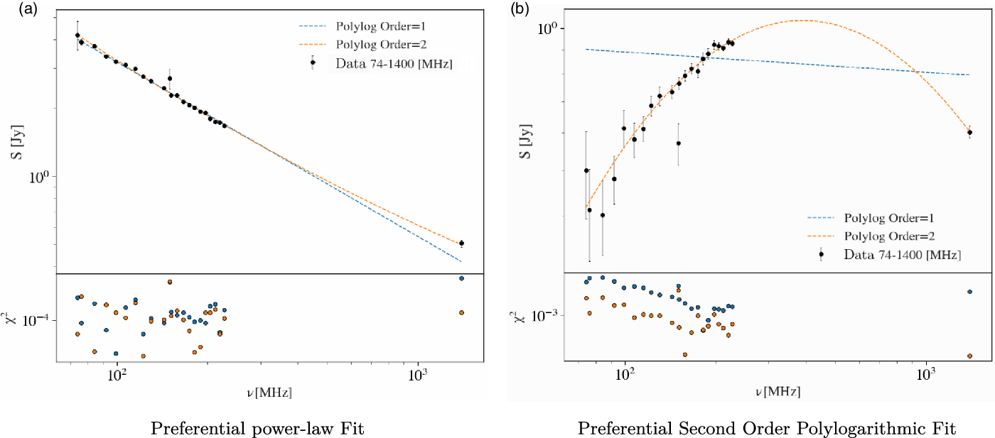
Log-log plot of the SED of representative sources taken from PUMAcat. In the top panel the black circles are the normalised flux densities as a function of frequency. The dashed blue line is the power-law fit to the SED (first order polylogarithmic fit), the dashed orange line is the second order polylogarithmic fit to the SED. The bottom panel shows the  $\chi^2$ normalised residuals for both fits as a function of frequency, where the colours correspond to the model in the top panel. Subfigure 3a shows a source with a preferred power-law fit, and Subfigure 3b shows a source with a preferred second order polylogarithmic fit.
3. 300 MHz sky-model
3.1. PUMAcat 300 MHz SED models
In this work we fit two models in log-space to the SEDs of radio sources in PUMAcat. These models allowed for the interpolation of the 300 MHz flux density. The first model we fit to each radio source was a power-law modelFootnote h:
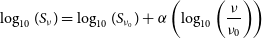 \begin{equation}\log_{10}(S_\nu) = \log_{10}(S_{\nu_0}) + \alpha \left( \log_{10}\left(\frac{\nu}{\nu_{0}}\right) \right)\end{equation}
where  $\nu_{0}$ is the reference frequency which we define at 300 MHz,
  $S_{\nu_0}$ is the flux density at the reference frequency, and
  $\alpha$ is the spectral index. Equation (1) in log-space is a straight line model, where the spectral index
  $\alpha$ is the gradient, and
  $\log_{10}(S_{\nu_0})$ is the y-intercept. For radio sources that only had two or three flux density measurements, we only fit the power-law model. The second model we fit is a second order polylogarithmic (polylog) function, this model is simply a parabola defined in log-space:
 \begin{equation} \log_{10}(S_\nu) = \log_{10}(S_{\nu_0}) + \alpha \left( \log_{10}\left(\frac{\nu}{\nu_{0}}\right) \right) + q \left( \log_{10}\left(\frac{\nu}{\nu_{0}}\right) \right)^2. \end{equation}
Equation (2) is the second order approximation of the radio source SEDs in log-space, where the parameter q is the curvature term of the parabola. This model is a natural choice, since many radio sources will display some curvature in their spectra across large enough frequency ranges (Callingham et al. Reference Callingham2017; Harvey et al. Reference Harvey, Franzen, Morgan and Seymour2018). The curvature term q provides a good approximation for sources intrinsic spectral curvature. Additionally q has also been linked to the magnetic field strength of active galactic nuclei (Bridle & Schwab Reference Bridle, Schwab, Taylor, Carilli and Perley1999). Radio sources with  $q<0$ indicate spectra with concaveFootnote i curvature, and radio sources with
  $q>0$ indicate spectra with convex curvature. The spectral index
  $\alpha$ in Equation (2) represents the steepness of the parabola at the reference frequency
  $\nu_{0}$. Other models such as broken power-law models do exist (Callingham et al. Reference Callingham2017), but Equation (2) is compatible with the calibration software used in this work, and adequately describes the SED in nearly all curved cases. The significance of this will be discussed further in Section 5.
The optimal fit parameters for Equations (1) and (2), are determined by minimising the  $\chi^2$ value for each fit. The
  $\chi^2$ is defined below:
 \begin{equation} \chi^2 = \sum^n_{i=0} \frac{\left(\log_{10}\left(S(\vec{\theta}|\nu_i)\right) - \log_{10}\left(S_{\textrm{data,i}}\right)\right)^2}{\sigma_i^2},\end{equation}
where  $S(\vec{\theta}|\nu_i)$ is the model at
  $\nu_i$ and
  $S_{\textrm{data},i}$ is the measured flux density at
  $\nu_i$. In Equation (3),
  $\vec{\theta}$ is a vector which contains the model fit parameters, and
  $\sigma_i$ is the uncertainty for
  $\log_{10}\left(S_{\textrm{data},i}\right)$. To perform the fit we use the numpy function polyfit in Python.
Model discernment between Equations (1) and (2) is performed by calculating the Bayesian information criterion (Schwarz Reference Schwarz1978, BIC):
 \begin{equation} \textrm{BIC} = \chi^2 + \ln{(n)}k.\end{equation}
The BIC takes into consideration the fit to the model  $\chi^2$, the number of data points n, and the number of model fit parameters k. The term
  $\ln{(n)}k$ penalises models with large numbers of parameters k. Models with too many parameters can overfit the data. For each radio source in PUMAcat, we calculate the
  $\textrm{BIC}$ for both models. We then compute the absolute difference
  $(\Delta\textrm{BIC})$ between the two models, this difference provides a relative comparison between the two fits. Values of
  $\Delta \textrm{BIC} \geq 6$ provide strong evidence that the model with the lower BIC, is the preferred fit to the data (Kass & Raftery Reference Kass and Raftery1995). When
  $\Delta \rm{BIC} < 6$ there is no significant evidence to select one model over the other. In this case the default preferred fit is Equation (1) since it has fewer fit parameters k.
Figure 3 illustrates two example SEDs. Subfigure 3a shows a source where Equation (1) is a preferred fit. Subfigure 3b shows a radio source with a concave SED, with Equation (2) being a clearly preferential fit. Once the sources were fit, and a preferential model was selected, we interpolated the 300 MHz flux density. The resulting sky-model at 300 MHz is hereon referred to as PUMA300.
3.2. GLEAM_Sup 300 MHz model
Radio sources in the GLEAM_Sup sky-model were fit using Equations 1 and 2, at a reference frequency of  $\nu_0 = 200\,\textrm{MHz}$ (Hurley-Walker et al., in prep). Since the GLEAM_Sup sky-model does not contain high frequency information, we extrapolated the flux density at 300 MHz using the model fit parameters. We did this by transforming the fit coefficients from a reference frequency of
  $\nu_0 = 200\,\textrm{MHz}$ to
  $\nu_0 = 300\,\textrm{MHz}$. The full fit coefficient transformation process can be found in Section B of the Appendix. For sources with second order polylogarithmic fits, the spectral index
  $\alpha_{200}$ is now defined at
  $\alpha_{300}$, where the subscript indicates the reference frequency in MHz.
3.3. TGSS/NVSS 300 MHz model
We interpolated the 300 MHz flux density for the TGSS/NVSS300 catalogue using a power-law:
 \begin{equation} S_{300} = S_{\rm{NVSS}}\left( \frac{300}{1\,400} \right)^{-\alpha}.\end{equation}
The spectral index in Equation (5) was determined by de Gasperin et al. (Reference de Gasperin, Intema and Frail2018) from the TGSS/NVSS catalogue. We use this spectral index along with the NVSS flux density  $S_{\textrm{NVSS}}$ from the TGSS/NVSS catalogue to interpolate the 300 MHz flux density.
We investigated systematic offsets in the interpolated TGSS/NVSS 300 MHz flux density, relative to the PUMA300 catalogue by performing a cross-match. In this case only single radio sources were considered because they are unresolved in both TGSS/NVSS and PUMA300. Using a cross-match separation of two arcminutes or less,  $176\,073$ matches were found. The ratio of the PUMA300 300 MHz flux density with the TGSS/NVSS estimate was computed, the flux ratio distribution can be seen in Figure 4. The median ratio of the distribution is
 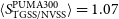 $\langle S^{\textrm{PUMA300}}_{\textrm{TGSS/NVSS}} \rangle = 1.07$ which is close to the expected value of 1.
The ratio of the PUMA300 and TGSS/NVSS 300 MHz flux densities is illustrated by the green histogram. The empty black dot dashed histogram, indicates the PUMA300 sources which were preferentially fit with a power-law  $(|q|=0)$. The empty solid red histogram shows the PUMA300 sources with a preferential second order polylogarithmic fit
  $(|q|>0)$. All histograms show a characteristic skew towards higher ratios, specifically for sources with
  $|q|>0$. The median flux ratio is shown as the dashed black line.
A ratio of  $\langle S^{\textrm{PUMA300}}_{\textrm{TGSS/NVSS}} \rangle>1$ indicates an underestimate in the 300 MHz flux density for the TGSS/NVSS catalogue. There are several potential contributing factors to the underestimate. The primary cause is likely due to the lack of curvature present in the TGSS/NVSS SEDs. In Figure 4 the distribution is broken into the power-law sources (
 $q=0$, black dashed line), and sources with curved SEDs (
 $|q|>0$, red line). The distribution with curved SEDs clearly has a larger tail at
  $\langle S^{\textrm{PUMA300}}_{\textrm{TGSS/NVSS}} \rangle>1$ when compared to the power-law source flux ratio distribution. The higher sensitivity of the GLEAM_Sup catalogue (and by extension PUMA300) to extended emission compared to TGSS and NVSS, would also contribute to the underestimate. Additionally there are systematic differences between the PUMA300 flux scale and the TGSS/NVSS flux scale that contribute to the underestimate. To correct for this average underestimate we use the median flux density ratio to scale the TGSS/NVSS300 flux densities.
3.4. Calibrator SED models
We consider calibrator source SED models separately due to their importance in calibrating MWA observations (Wayth et al. Reference Wayth2015; Hurley-Walker et al. Reference Hurley-Walker2017). The total estimated 300 MHz flux density for each calibrator source was interpolated using SED models fit by Perley & Butler (Reference Perley and Butler2017). These models were developed to investigate the flux scale of calibrator sources from  $50\,\rm{MHz}$ to
  $50\,\rm{GHz}$. The models were developed by fitting arbitrary order polylogarithmic functions at a reference frequency of
  $\nu_0 = 1\,\rm{GHz}$ to VLA data (Perley & Butler Reference Perley and Butler2017). Using the coefficient transformation method discussed in the Appendix Section B, we transformed the fit coefficients for the calibrator sources to a reference frequency of
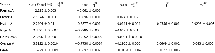
  $\nu_0 = 300\,\textrm{MHz}$. The transformed polylogarithmic fit coefficients for the total calibrator SEDs can be found in Table 3.
Each calibrator source contains multiple components, but to simplify the approach we assume that each component has the same SED as the total radio source. For simple resolved two point source galaxies such as Pictor A or unresolved calibrators sources such as 3C444, assuming the total SED was the same for each of the components was a reasonable assumption. This assumption allowed for the creation of first pass calibration solutions for 300 MHz observations in Cook (Reference Cook2020). We calculate the 300 MHz flux density for each component as a fraction of the total source flux density  $S_{\textrm{tot},300}$. This fraction is determined from the bespoke models described in Section 2.4, where the flux density of each component is summed at the frequency of the cutout image
  $S_{\textrm{tot},\nu}$. The fraction for each component is then determined, and multiplied by the total estimated 300 MHz flux density from the Perley & Butler (Reference Perley and Butler2017) SED models. More accurate component source models will be the focus of future work.
The polylogarithmic coefficients for each of the calibrator sources at a reference frequency of  $\nu_0 = 300\,\textrm{MHz}$. These were determined by transforming the polylogarithmic coefficients from Perley & Butler (Reference Perley and Butler2017) from
 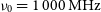 $\nu_0 = 1\,000\,\textrm{MHz}$ to
  $\nu_0 = 300\,\textrm{MHz}$. Column two is the estimated
  $\log_{10}$ flux density in Janksy’s for each calibrator source. Columns three and four show the spectral index
  $\alpha_{300}$ and curvature term
  $q_{300}$ for each source were applicable. Columns five and six are the higher order polylogarithmic coefficients. These last columns demonstrate the level of curvature present in radio SEDs.
3.5. Total 300 MHz catalogue
The columns for each component catalogue were standardised and concatenated together. The new combined 300 MHz sky-model catalogue contains  $433\,345$ table entries, and is hereon referred to as Total300. Table 4 provides the column format for the Total300 sky-model catalogue. Using the method outlined in the Appendix Section B, Total 300 can be transformed from a 300 MHz sky-model to one in the frequency range
  $72-1\,400\,\rm{MHz}$. The Total300 sky-model and the transformation script are publicly available through the GitHub repository associated with this work S300-pipelineFootnote j.
Table 5 breaks down the statistics for the component catalogues of Total300 (not including the calibrator models). The fraction of sources with  $|q_{300}| > 0$ for the combined PUMA300 and GLEAM_Sup models is
  ${\sim}0.163$. The GLEAM_Sup sources predominantly have positive curvature because they lack the high frequency information.
4. Observations
We use publicly available 2 min MWA Phase I snapshot observations, which can be downloaded from the MWA All-Sky Virtual Observatory (ASVO)Footnote k server using the MWA manta-rayFootnote l python client (Sokolowski et al. Reference Sokolowski2020). The raw observation files are downloaded and consolidated into a measurement set using the software cotter (Kemball & Wieringa Reference Kemball and Wieringa2000; Offringa et al. Reference Offringa, Wayth and Hurley-Walker2015). cotter averages MWA observation data in time and frequency, it additionally flags RFI using the aoflagger algorithm (Offringa, van de Gronde, & Roerdink, (Reference Offringa, van de Gronde and Roerdink2012)). aoflagger was found to be inadequate at flagging most of the RFI at 300 MHz. In particular there is a high RFI occupancy in the lower coarse channels, as found by Sokolowski et al. (Reference Sokolowski, Wayth and Lewis2015). As a result the first four coarse channels for every 300 MHz observation typically have to be flagged. We additionally expanded our flagging regime through the common astronomy software applications (CASA)Footnote m package (McMullin et al. Reference McMullin, Waters, Schiebel, Young and Golap2007). We use the CASA RFI flagging functions rflag and tfcrop (refer to McMullin et al. (Reference McMullin, Waters, Schiebel, Young and Golap2007) for a detailed description of these algorithms). Further flagging per baseline is also required, since some baselines have a high occupancy of RFI. To flag these baselines another flagging tool referred to here as steflagFootnote n is used (Duchesne Reference Duchesne2019). This tool flags baselines using their statistics to identify outliers, it then outputs a list of antenna pairs which can be passed to CASA for flagging.
Column format of the Total300 sky-model catalogue.
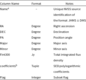
aThe naming convention takes exception to calibrator sources where the format of their names is laid out in subsection 2.4.
bThe coefficients are formatted in a tuple of size 6, where  $(a_0, a_1,\cdots,a_6)$, sources with only power-law or second order polylogarithmic fits have coefficients
  $a_3$ to
  $a_6$ set at 0.
Median values of the SED fits for the three main subsets of the Total300 sky-model. The calibrator sources are not included here except for the total number of table entries.
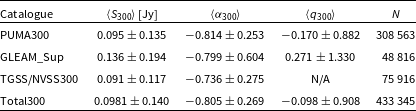
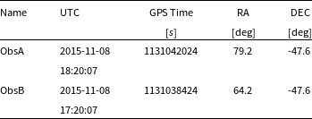
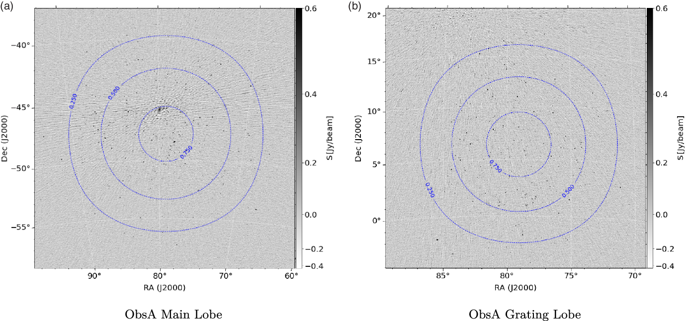
Table 6 lists the snapshot 300 MHz MWA observations used to demonstrate the imaging and calibration strategy outlined in this work. These observations were taken during an extended observing run, in the second year of GLEAM. ObsA is a calibrator observation of the calibrator radio galaxy Pictor A. ObsB was taken an hour before ObsA during the same observing night. Both observations have the same pointing. In this work we use ObsA as a calibrator observation to calibrate ObsB.
List of example observations used in this work. The UTC, GPS, RA and DEC of the observation phase centres are provided for both observations. These observations are publicly available.
4.1. ObsA & ObsB primary beam pattern
The primary beam for ObsA and ObsB has a phase centre of  $\phi = 180^{\circ}$, and
  $\theta_\textrm{zen} = 20^{\circ}.84$. The primary beam pattern as projected across the whole sky can be seen in left panel of Figure 5 where the phase centre (which is also the centre of the main lobe) is indicated by the solid red circle. Since the primary beam is pointed away from zenith, the projection of the grating lobes and their relative sensitivities is different from the zenith projection. For instance, there are only three apparent grating lobes, the southernmost grating lobe has disappeared, and the northernmost grating lobe has increased in prominence (this is similar to the phenomenon demonstrated in Figure 1). For this projection, the peak sensitivity of the prominent grating lobe across the bandwidth is approximately as sensitive as the main lobe, the centre of which is indicated by the solid red triangle in Figure 5.
The left panel is the orthographic MWA FEE primary beam model for ObsA, where the solid black contour lines are shown on the log-scale colour bar and are the same as those in Figure 1. The dashed black lines are constant zenith lines. The right panel is the difference between the primary beam at the top of the band compared to the bottom of the band. The main lobe is shown with the large red filled circle, the approximate centres of the grating lobes are shown with the red filled crosses, and the prominent grating lobe is shown with the red filled triangle. The min beam difference is  ${\sim}-0.5$, we restrict the beam difference colourbar scale to
  $[{-}0.2,0.2]$.
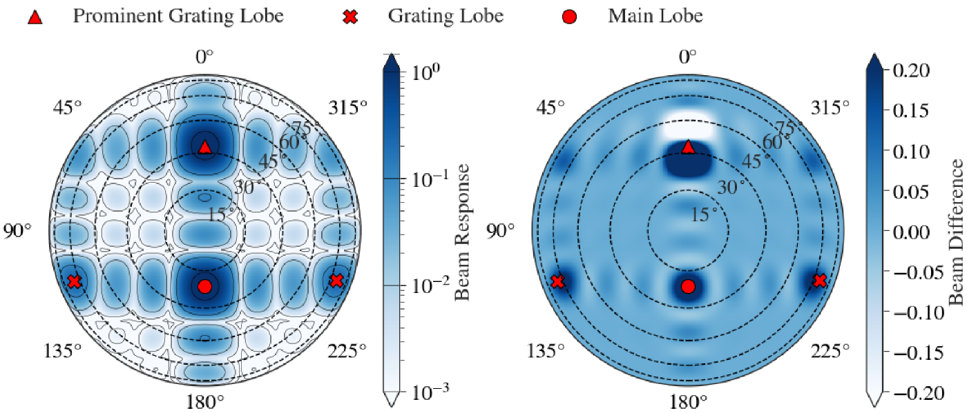
This observation demonstrates the challenges of imaging at 300 MHz with the MWA. The prominent grating lobe effectively means there are two main fields of view. This can also be a potential benefit because the prominent grating lobe in this case could be imaged. However, exploiting the grating lobes for science is beyond the scope of this initial work. Additional challenges arise with grating lobes as a result of how they change as a function of frequency across the bandwidth. This can be seen in the right panel of Figure 5 where we show the difference between the highest coarse channel and lowest coarse channel primary beam patterns. Clearly the prominent grating lobe undergoes a shift towards the main lobe as a function of increasing frequency. Inaccuracies in the beam model for sources in the grating lobes will result in incorrect flux measurements.
5. 300 MHz calibration strategy
300 MHz MWA calibrator observations are calibrated using the software package calibrate (Offringa et al. Reference Offringa2016). This software takes a model of the apparent sky as a function of frequency, and uses this model to predict the visibilities for that observation. calibrate then performs a minimisation with the measured visibilities to determine the instrumental gain and phase solutions (Mitchell et al. Reference Mitchell, Greenhill, Wayth, Sault, Lonsdale, Cappallo, Morales and Ord2008). Once derived, the solutions can then be applied to the interferometric data for that observation, or for other observations at the same pointing. The apparent sky-model required to determine the gain amplitude and phase solutions, can be constructed from the Total300 catalogue and the FEE MWA tile beam model (Sokolowski et al. Reference Sokolowski2017). Each observation will have a different ‘apparent sky-model’ due to differing LST, and RA/DEC of the phase centre.
5.1. Constructing the apparent sky-model
Each snapshot observation has a particular UTC time, this can be used in conjunction with the RA and DEC to determine the  $\theta_\textrm{zen}$ and
  $\phi$ angles for each source in the Total300 catalogue. Sources below the horizon
  $(\theta_\textrm{zen} > 90\,^{\circ})$ are removed. The integrated flux density for the remaining sources is then attenuated by the 300 MHz MWA FEE tile beam response. The brightest 1 500 sources are then selected, these sources constitute the base of the apparent sky-model. A model of the apparent flux density
  $S_\textrm{app}(\nu)$ as a function of frequency for the remaining 1 500 sources is required by calibrate in order to predict the observation visibilities, and is defined as:
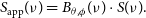 \begin{equation} S_{\textrm{app}}(\nu) = B_{\theta,\phi}(\nu) \cdot S(\nu).\end{equation}
Equation (7) incorporates the intrinsic source SED model  $S(\nu)$, and the spectral structure of the MWA tile primary beam response
  $B_{\theta,\phi}(\nu)$, which is determined at the source’s position
  $(\theta,\phi)$. Additionally for snapshot observations we assume that at a fixed
  $(\theta,\phi)$ that the sky is approximately constant, therefore
  $B_{\theta,\phi}(\nu)$ is also constant. One type of
  $S_\textrm{app}$ model calibrate accepts is arbitrary order polylogarithmic functions similar to the models used by Perley & Butler (Reference Perley and Butler2017). Equation (7) is the general model we use in this work:
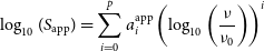 \begin{equation} \log_{10}(S_{\textrm{app}}) = \sum^p_{i=0} a^\textrm{app}_i \left( \log_{10} \left(\frac{\nu}{\nu_0} \right) \right)^i\end{equation}
p is the polynomial order, and  $\nu_0$ is the same reference frequency from Section 3.1. Equation (7) can also be expressed as a linear combination of two polylogarithmic functions
  $\log_{10}(S(\nu))$ and
  $\log_{10}(B_{\theta,\phi}(\nu))$ in log-space.
  $\log_{10}(B_{\theta,\phi}(\nu))$ is modelled as a polylogarithmic function to interpolate the MWA fine channel beam response for a particular source. This is done because the FEE tile beam model only models the coarse channels of the tile beam response (Sutinjo et al. Reference Sutinjo, O’Sullivan, Lenc, Wayth, Padhi, Hall and Tingay2015; Sokolowski et al. Reference Sokolowski2017). In many cases higher order polylogarithmic functions are required to accurately interpolate
  $\log_{10}(B_{\theta,\phi}(\nu))$ for a particular source. This is a result of some bright sources being located near MWA tile beam nulls where the beam response is changing quickly. An extreme example of a source near an MWA tile beam null is illustrated in Figure 6.
One of the more extreme examples of log-beam curvature across the 300 MHz bandwidth. The individual black points are the coarse channels in the bandwidth. The beam response shows multiple changes in the gradient as well as minima. Several log-space polynomials were fit to the log-beam coarse channels, in this figure we only show the odd ordered polynomials. These are represented by the coloured dashed lines.
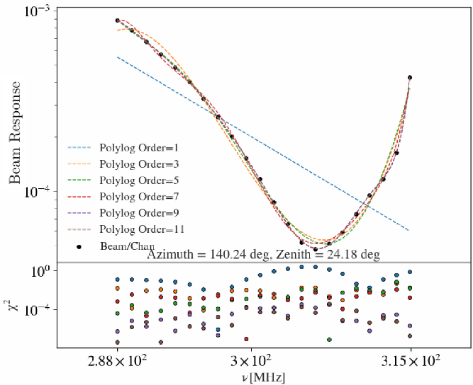
The choice of polynomial order fit to  $\log_{10}(B_{\theta,\phi}(\nu))$ depends on the location of the source in the beam response. In most cases the 11th order polynomial required to accurately model the beam response in Figure 6 is not necessary. Generally a simple first order to fifth order polynomial is appropriate to model
  $\log_{10}(B_{\theta,\phi}(\nu))$. To choose the appropriate order fit, we calculate the
  $\chi^2$ value from Equation (3), with a
  $\sigma = 1$; we additionally determine the degrees of freedom
  $(\textrm{dof} = N - (p + 1))$. We use the minimisation of the
  $\chi^2$ and the
  $\textrm{dof}$ to select an appropriate polynomial order fit to
  $\log_{10}(B_{\theta,\phi}(\nu))$. We limit the maximum order fit polynomial to
  $p \leq 11$, above this limit over-fitting starts to become an issue, and interpolation becomes increasingly inaccurate due to the Runge phenomenon (Epperson Reference Epperson1987).
Once the log-beam coarse channels have been fit for every source, we add the  $\log_{10}(B_{\theta,\phi}(\nu))$ fit coefficients to the
  $\log_{10}(S(\nu))$ coefficients to determine the apparent coefficients in Equation (7). The sources along with their fit coefficients are then written to a to a VOTable (Ochsenbein & Williams Reference Ochsenbein and Williams2009). An example apparent sky-model 300 MHz image generated from the output VOTable can be seen in Figure 7. Figure 7 shows the main lobe and the most prominent grating lobe from the apparent sky-model of the calibrator observation ObsA, the primary beam contours are overlaid in dashed blue lines.
Image of the apparent sky-model for ObsA, Subfigure 7a shows the main lobe of the observation, centred at  $\textrm{RA}=79^{\circ}.95$,
 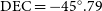 $\textrm{DEC}=-45^{\circ}.79$. Pictor A is visible in the enlarged box in the bottom left hand corner. Subfigure 7b shows the prominent grating lobe for ObsA centred at
  $\textrm{RA}=79^{\circ}.95$,
  $\textrm{DEC}=+5^{\circ}$.
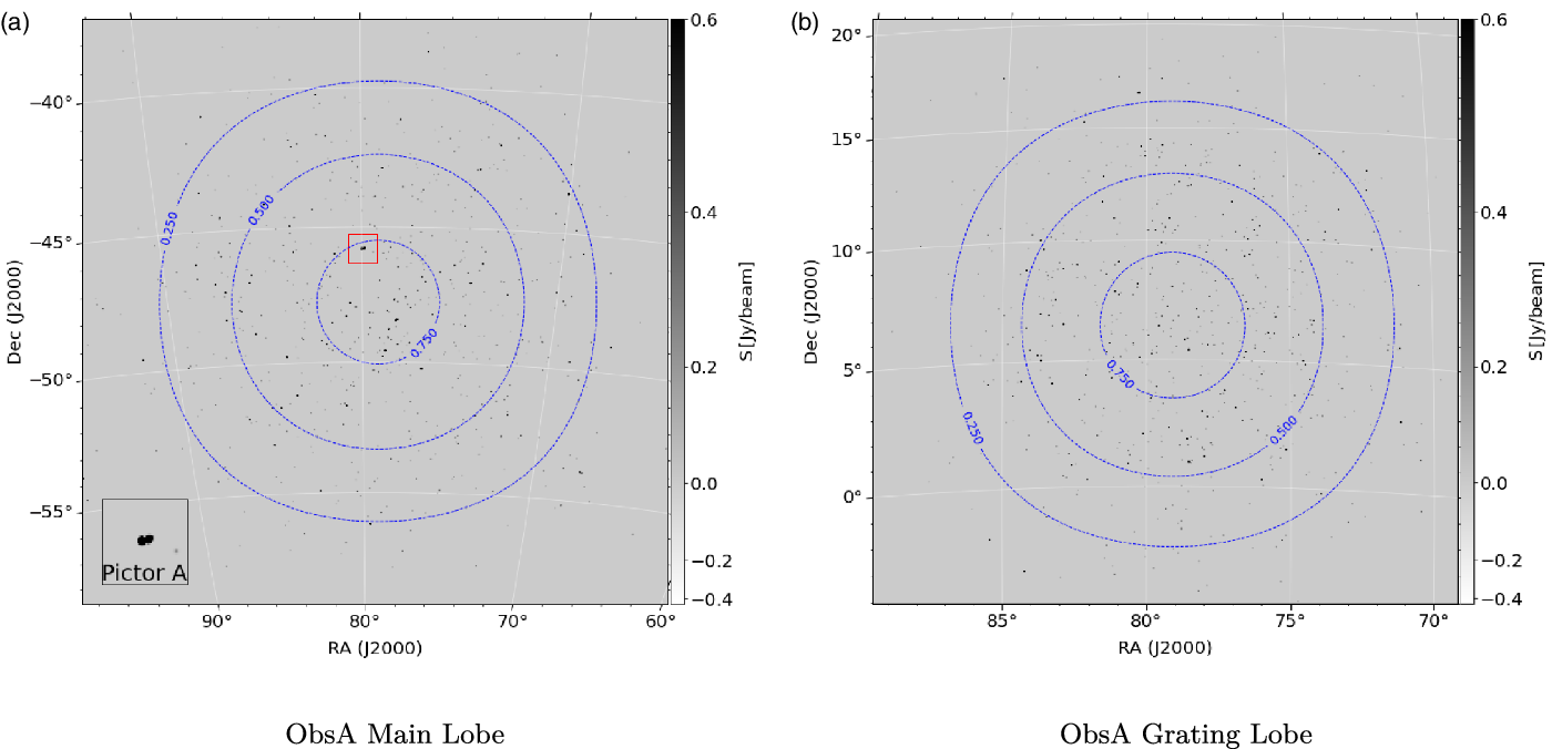
Apparent all-sky image of ObsA, presenting the main lobe, and the most prominent grating lobe. Subfigure 8a shows the main lobe centred at  $\textrm{RA}=79^{\circ}.95$,
  $\textrm{DEC}=-45^{\circ}.79$ with an rms of
  $86\,\textrm{mJy/beam}$. Subfigure 8b shows the most prominent grating lobe centred at
  $\textrm{RA}=79^{\circ}.95$,
  $\textrm{DEC}=+5^{\circ}$ with an rms of
  $68\,\textrm{mJy/beam}$. The restoring beam for both images has a major axis size of
  ${\sim}2.3\,\textrm{arcmin}$, and a minor axis of
  ${\sim}2.1\,\textrm{arcmin}$. There are additional grating lobes to the east and west of the main lobe which contain additional sources. Since the projection of this observation is significantly away from zenith, these grating lobes are significantly less prominent than the one shown in Subfigure 8b. As such they were not included.
5.2. Calibrating the apparent sky-model
The VOTable formatted apparent sky-model is converted into a text file, with a format specific to calibrate. This sky-model text document is a list from brightest to faintest of the 1 500 selected sources. Each source in the list contains information about its RA and DEC, and the sources integrated apparent flux density at  $300\,$MHz. If the source is a Gaussian it also provides the major and minor axes in arcseconds, as well as the position angle of the source clockwise relative to North in degrees. The apparent flux density coefficients for each source are additionally given.
This text file along with the observation measurement set are passed to calibrate, which is executed on uncalibrated visibilities and outputs the solutions to a binary file (Offringa et al. Reference Offringa2016). applysolutionsFootnote o is used to apply calibration solutions to the same or other observations (Offringa Reference Offringa2019). After the initial calibration, we perform another round of RFI flagging. This flags calibration outliers and any additional RFI that is more prominent after initial calibration.
5.3. All-sky imaging & self-calibration
The apparent sky-model for calibrator observations provides a good first pass calibration of the observation visibilities, these can then be used to create deconvolved all-sky images (Högbom Reference Högbom1974). In this work all-sky imaging is performed with the software package wsclean (Offringa et al. Reference Offringa2014). wsclean takes into account the w-terms for MWA observations due to the wide field of view, with a process called w-stacking (Humphreys & Cornwell Reference Humphreys and Cornwell2011). The resulting CLEAN components generated from the all-sky images may then be used to perform another round of self-calibration.
To perform the all-sky imaging the visibilities are first phase shifted to zenith using the wsclean software chgcentre (Offringa et al. Reference Offringa2014). The resulting zenith phase shifted visibilities reduce the w-terms, and are capable of producing an orthographic image of the entire sky. We then perform a shallow CLEAN using a uniform weighting with wsclean, with a threshold of  $0.3$, an auto mask of
  $3.0$ and an mgain of
  $0.85$. Due to the high computation costs of performing deconvolution on high resolution all-sky images, we limit wsclean to
  $300\,000$ minor iterations. The image size is additionally limited to
  $7\,000$ by
  $7\,000$ pixels due to memory constraints.
Since the all-sky image is an orthographic projection, the projected diameter for the celestial sphere of unit radius is  $114^{\circ}.58$ (this is equivalent to two radians in degrees). Dividing this by the number of pixels along one dimension determines a pixel resolution of
  $\Delta\theta = 59\,\textrm{arcsec}$. The expected PSF at
  $300\,\textrm{MHz}$ is
  ${\sim} 1.2\,\textrm{arcmin}$, which provides an effective pixel sampling of
  $1.2$ pixels per PSF. Due to the constraints on the image size and thus the resolution, we use wsclean to convolve the PSF with a Gaussian of size
  $140\,\textrm{arcsec}$. This provides an effective PSF sampling rate of
  ${\sim}2.4$ pixels per PSF, and a resolution which is comparable to the GLEAM wide-band resolution (Hurley-Walker et al. Reference Hurley-Walker2017). Loss in sensitivity due to down weighting longer baselines is negligible since most baselines
  $(\geq 90 \%)$ are shorter than
  ${\sim}1\,432\,\textrm{m}$. There may additionally be slight sensitivity gains to large angular scales as a result of up weighting shorter baselines.
Examples of the main lobe, and the grating lobe from the apparent all-sky image of ObsA can be seen in Figure 8. Subfigure 8a shows the main lobe which has an rms sensitivity of  $86\,\textrm{mJy/beam}$, the noise here is dominated by the sidelobes of Pictor A. Subfigure 8b is the most prominent grating lobe which contains numerous radio sources, some of which are very bright. The rms sensitivity at the centre of the grating lobe is
  $68\,\textrm{mJy/beam}$, which is lower than the main lobe due to the lack of high sidelobe noise. In the absence of sidelobe confusion noise, the rms sensitivity at the centre of both lobes is expected to be approximately the same.
During the CLEAN process wsclean generates a model where it stores the CLEAN component visibilities (Offringa et al. Reference Offringa2014). calibrate can use the CLEAN component model visibilities to calibrate the data. For calibrator observations which have high signal to noise, the resulting gain and phase solutions are often better constrained. These solutions can be applied to the calibrator observation, or to a non-calibrator observation at the same pointing. After they have been applied an additional round of RFI/outlier flagging is performed.
6. Main lobe imaging strategy
In radio interferometry, the main lobe of an observation (which determines the field of view), is typically the principal scientific region of interest. The presence of several highly sensitive grating lobes at 300 MHz for MWA observations, means there are effectively several fields of view for a given observation. The radio sources which are present in these grating lobes produce sidelobe confusion that lowers the dynamic range of the main lobe. To properly image the main lobe, the contribution to the visibilities from the remaining parts of the sky need to be subtracted. In this section we describe the sky-subtraction and imaging process for the main lobes of 300 MHz observations. In principle this process can be generalised for any lobe, but for this work we only focus on the main lobe.
Beam corrected Briggs  $0.0$ weighted main lobe images for ObsA and ObsB in Subfigure (a) and (b) respectively. In Subfigure (a) the enlarged region shows Pictor A which at the resolution of this image is unresolved. Faint sidelobe artefact can be seen in both images, where the rms for Subfigure (a) is
  $56\,\textrm{mJy/beam}$ and
  $31\,\textrm{mJy/beam}$ for Subfigure (b). The restoring beam size is
  ${\sim}2.3\,\textrm{arcmin}$, by
  ${\sim}2.1\,\textrm{arcmin}$. The deeper rms for Subfigure (b) is a result of the absence of Pictor A in the main lobe.
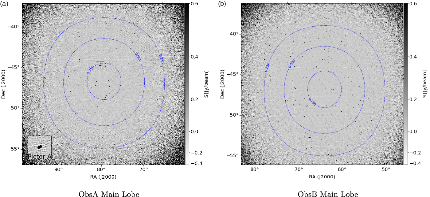
6.1. Sky-subtraction algorithm
To image the main lobe we developed a method which uses wsclean to remove the sky contribution from the visibilities. In the process of imaging the entire sky (described in Section 5.3), wsclean outputs the CLEAN model components to an image with the same dimensions as the output all-sky image (Offringa et al. Reference Offringa2014). Using the wsclean predict function the visibilities of this image can be estimated, and written to the model column of the observation measurement set. To separate the main lobe contribution to the visibilities from the rest of the sky, we mask the main lobe in the model image by setting all pixel values to zero. We then run predict function on the masked image. Using the wsclean taqlFootnote p command the model visibilities are subtracted from the calibrated visibilities. We then perform another round of all-sky imaging, this will CLEAN the sources that were missed in the original run (at the cost of extra computation). This process can be iteratively repeated, but the default number of iterations is one. After each imaging stage we flag any additional RFI and calibration outliers.
6.2. Main lobe image parameters
After the sky-subtraction process is performed the main lobe of the observation is imaged using wsclean. Main lobe images are by default generated with a Briggs weighting of  $0.0$, using the wslean multi-scale CLEAN option (Offringa & Smirnov Reference Offringa and Smirnov2017). The additional default imaging options are an auto threshold of 1, with an auto mask of 3, and an mgain of
  $0.5$ for
  $500\,000$ minor iterations. Output images have dimensions of
  $5\,000$ by
  $5\,000$ pixels, with a pixel scale of
  $\Delta\theta {\sim} 18\,\textrm{arcsec}$. At this pixel scale, an untapered PSF of
  ${\sim}1.3\,\textrm{arcmin}$, corresponds to a pixel sampling of four pixels per PSF. For comparison with the main lobe cutout image from the all-sky image in Figure 9a we also taper the main lobe image PSF to a resolution of
  ${\sim}2.4\,\textrm{arcmin}$.
7. Results
In this section we present the output main lobes images for the calibrator observation ObsA, and a non-calibrator observation ObsB, which we calibrated using solutions derived from ObsA. We apply the process outlined in Sections 5 and 6 to these two example observations to illustrate the calibration and imaging strategy, the main lobe images of ObsA and ObsB are shown in Figure 9a and 9b respectively.
Difference in the RA and DEC between the model and the measured sources for ObsA (Subfigure 10a) and ObsB (Subfigure 10b). The dashed black lines for both figures show how far the sources deviate from an offset of zero. The colour bar shows the estimate probability density for both figures.
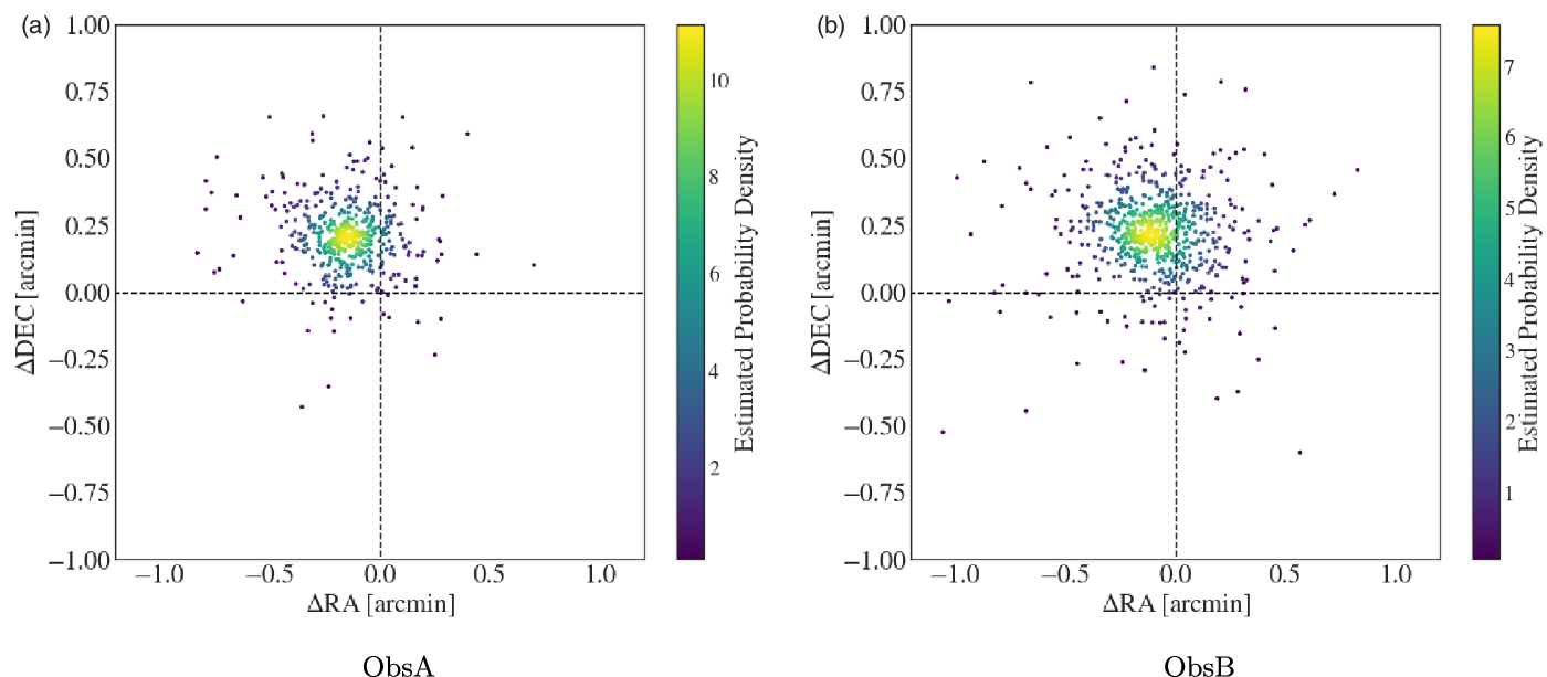
7.1. ObsA & ObsB main lobe images
Comparing the sensitivity of the ObsA main lobe image from Figures 9a–8a, the former clearly has many more visible point sources. The rms in Figure 9a is  $56\,\textrm{mJy/beam}$ compared to
  $86\,\textrm{mJy/beam}$ in Figure 8a. The majority of the improvement in sensitivity comes from eliminating sidelobe confusion, through the application of the sky-subtraction method, and by performing a deeper CLEAN on Pictor A. Additional gains in sensitivity come from using a Brigg’s weighting of
  $0.0$, which balances resolution for an increase in sensitivity. Further gains in sensitivity come from removing RFI after applying the all-sky imaging and subtraction phase.
For ObsA and ObsB the total flagged visibilities percentage is  ${\sim}46\%$. Referring to Equations (8) and (11) of Section A in the appendix, for a naturally weighted observation with
  ${\sim}46\%$ flagged data, the best sensitivity for a snapshot 300 MHz observation is
  ${\sim}26\,\textrm{mJy/beam}$. In Subfigure 9a there are still sidelobes present for Pictor A, which will be contributing to the noise through sidelobe confusion. For ObsB since Pictor A is not present in the main lobe, the main lobe sensitivity is
  $31\,\textrm{mJy/beam}$. When accounting for the different weighting schemes and potential flux scale calibration errors, the sensitivity limit for ObsB is close to the theoretical prediction.
7.2. ObsA & ObsB astrometry
With the deep main lobe images for ObsA and ObsB we investigate the accuracy of the source positions relative to the Total300 catalogue. Using the source finder aegean we create source lists for ObsA and ObsB (Hancock et al. Reference Hancock, Murphy, Gaensler, Hopkins and Curran2012; Hancock, Trott, & Hurley-Walker, Reference Hancock, Trott and Hurley-Walker2018). The total number of sources found by aegean were 457 for ObsA and 656 for ObsB respectively. These source lists are then cross-matched with the Total300 catalogue at an angular separation of two arcminutes. The cross-matching is performed by the astronomy software topcatFootnote q (Taylor Reference Taylor, Britton, Britton and Ebert2005). The resulting cross-matched catalogues for ObsA and ObsB constitute a completeness of  ${\sim}99\%$. Due to the low sensitivity threshold for the ObsA and ObsB main lobe images, we should expect to see 100% cross-match with Total300 and the aegean source catalogues. Sources that do not have a match are potentially artefacts, or have peaks in their spectrum at higher frequencies. High frequency peaked sources, would be fainter at lower frequencies.
Using the cross-matched catalogue we determine the angular offsets for the sources in RA  $(\Delta\textrm{RA})$ and DEC
  $(\Delta\textrm{DEC})$. The resulting astrometry plots for ObsA and ObsB are given in Figure 10. There is a clear median bulk offset of
  ${\sim} 15\,\textrm{arcsec}$ for both ObsA and ObsB in Figure 10. The standard deviation for
  $\Delta\textrm{RA}$ for ObsA and ObsB is
  $7.8\,\textrm{arcsec}$ and
  $10.2\,\textrm{arcsec}$ respectively. The standard deviation for
  $\Delta\textrm{DEC}$ for ObsA and ObsB is
  $5.4\,\textrm{arcsec}$ and
  $7.2\,\textrm{arcsec}$ respectively. There does not appear to be any correlation between the RA and DEC offsets.
A potential cause for these offsets comes from the bespoke calibrator source models. These were created from the cutout  $227\,\textrm{MHz}$ GLEAM images which have pixel sizes of
  ${\sim}24\,\textrm{arcsec}$. Depending on where the pixel centre is defined this would affect the bespoke model positions, and a systematic offset of
  $\pm {\sim}12\,\textrm{arcsec}$ could be introduced. Similar offsets were observed for a
  $300\,\textrm{MHz}$ MWA calibrator observation of 3C444 in Cook (Reference Cook2020). The model for 3C444 in this observation was created using the same bespoke point source method used for Pictor A. Ionospheric shifts may also be responsible for some of the bulk offset, at
  $300\,\textrm{MHz}$ the worst case scenario shifts would be
  ${\sim}9\,\textrm{arcsec}$ (Smith Reference Smith1952; Thompson Reference Thompson2017; Jordan et al. Reference Jordan2017). Both bespoke calibrator model position errors and ionospheric effects are contributors to the bulk offset such as that seen in Figures 10a and 10b. However this systematic shift in positions is inconsequential to the strategy outlined in this paper, and is easily corrected for. In future work the input sky-model will be updated upon the release of higher resolution MWA extended baseline Phase II sky surveys such as GLEAM-X (Hurley-Walker et al., in prep) and the Long Baseline EoR Survey (LoBES; Lynch et al., submitted).
Scatter plot of the flux density ratio for cross-matched ObsA and ObsB source in blue against RA (Subfigures 11a and 11c) and DEC (Subfigures 11b and 11d). The dashed black line indicates the median flux density ratio for both ObsA and ObsB. There is no apparent trend with either RA or DEC. Notable outliers are present in the bottom left-hand corner of Subfigure 11c. These sources are close to the edge of the main lobe, they also appear in the bottom of Subfigure 11d
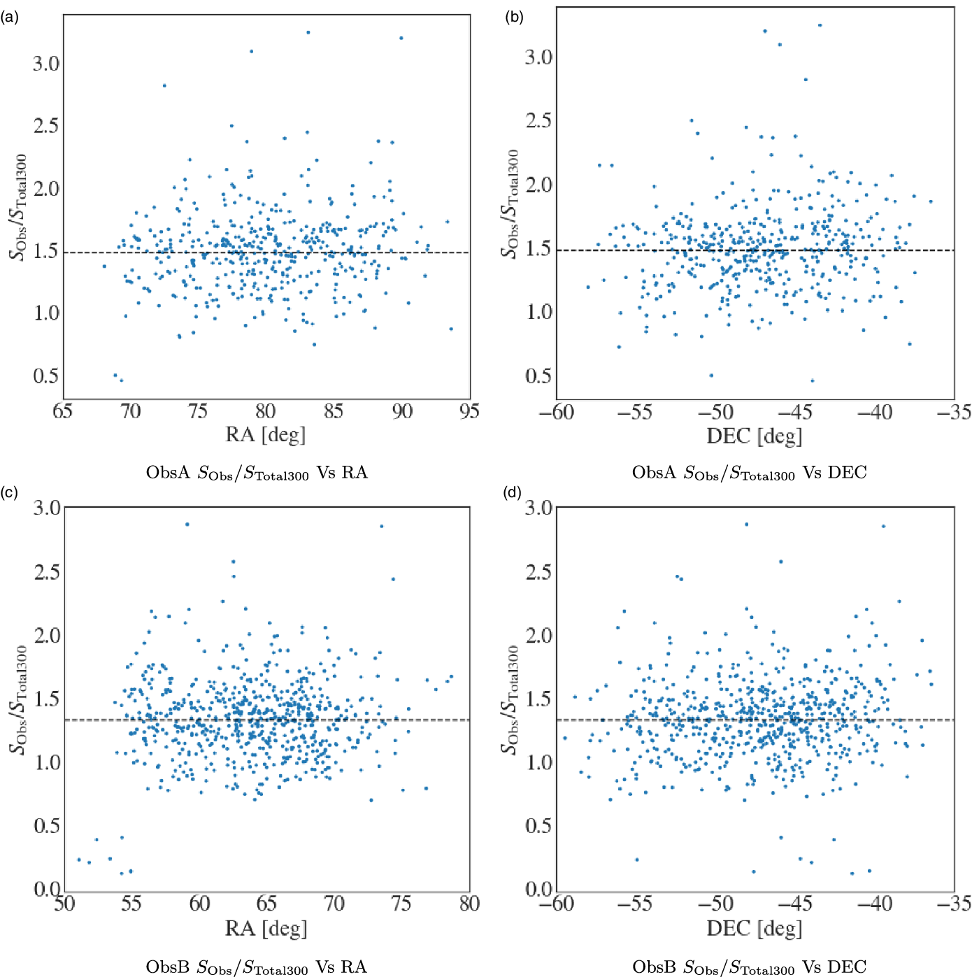
7.3. ObsA & ObsB flux scale
Using the cross-matched catalogues, the flux scale for ObsA and ObsB was determined by taking the ratio of the measured integrated flux density  $(S_\textrm{Obs})$ determined by aegean, to the Total300 model integrated flux density
  $(S_\textrm{Total300})$. The median flux density ratio for ObsA is
  $1.48\pm0.26$, and
  $1.33\pm0.25$ for ObsB respectively. The deviation from a unitary flux density ratio indicates there is an error in the flux scale calibration. This could potentially result from underestimating the total flux density in the calibrator observation ObsA. The scatter plots in Figure 11 show the flux density ratio plotted against RA and DEC for both ObsA and ObsB. There does not appear to be any systematic bias in the flux density in relation to either RA or DEC for either observation. In Figure 11c and 11d there appears to be a cluster of outlier sources with flux density ratios less than
  $0.5$. These sources are close to the edge of the main lobe, which could be indicative of an incorrect primary beam correction.
Flux scale issues associated with the primary calibrator sources might explain the offset, however the flux scale ratio for Pictor A in ObsA is  ${\sim}1.4$ close to the median offset. In Cook (Reference Cook2020) we investigated the flux scale ratios for several 300 MHz MWA calibrator and non-calibrator observations. The median flux scale ratios for these observations ranged from
  ${\sim}1.0$ to
  ${\sim}1.5$, for the calibrator sources 3C444, and Pictor A. The best median flux scale was
  ${\sim}1.0$ seen for the 3C444 calibrator observation. Cook (Reference Cook2020) also applied the calibration strategy to an observation of the GAMA 23 field which has no bright calibrator source, and found a median flux scale ratio of
  ${\sim}1.4$. These preliminary results seem to indicate that flux scale offsets affect both calibrator and non-calibrator observations. Since only a single snapshot observation was tested for each observation in Cook (Reference Cook2020) it is impossible to tell if these offsets would have the same effect for other snapshot calibrator observations. These flux scale offsets however are a common feature for MWA snapshot observations at other frequencies, and often image based corrections are applied to observations to correct for these flux scale issues (Wayth et al. Reference Wayth2015; Hurley-Walker et al. Reference Hurley-Walker2017). These issues arise from a myriad of systematic sources, in particular sky-model errors, and inaccuracies of the MWA FEE primary beam model which can introduce errors on the order of %10 (Sokolowski et al. Reference Sokolowski2017). Beam errors in particular are worse at higher frequencies due to the increased mutual coupling between individual MWA tile dipoles (Sutinjo et al. Reference Sutinjo, O’Sullivan, Lenc, Wayth, Padhi, Hall and Tingay2015). Other flux scale offsets can occur during the self-calibration process performed by wsclean and calibrate; self-calibration is often omitted from the current MWA observation processing paradigm. Future all-sky survey data releases for both the MWA and higher frequency arrays will offer better resolution and higher frequency data required to make more accurate sky-models, and calibrator source models.
8. Discussion and conclusion
The purpose of this paper was to demonstrate that MWA observations at 300MHz could be calibrated using a sky-model approach, and to offer a strategy for processing 300MHz observations. In this work we demonstrate a calibration and imaging strategy for 300 MHz MWA observations, and the processing pipeline used in this work is publicly available in the GitHub repository S300-pipelineFootnote r. To date this pipeline has successfully processed over 15 300 MHz observations (Cook Reference Cook2020), and is flexible enough to also process MWA observations at lower frequencies. The strategy outlined in this paper works best when calibrating a bright calibrator source, and then transferring the solutions to another observation at the same pointing. Some observations of relatively low brightness fields can be calibrated without a calibrator observation, but in practice with the current sky-model and beam model this is can be difficult.
There are many difficulties associated with processing 300 MHz MWA data. In particular RFI was a larger issue than anticipated. Each processing step required additional flagging to remove the RFI contribution to the visibilities. In particular we found that the coarse channels around  $280\,\textrm{MHz}$ had high levels of RFI occupancy and were entirely flagged, this is in agreement with the published RFI environment results of
  ${\sim}80\%$ RFI occupancy at these frequencies by (Sokolowski et al. Reference Sokolowski, Wayth and Lewis2015). Additionally some observations show evidence of intervening satellites which either reflect or transmit at the lower frequency coarse channels in the 300 MHz band; Cook (Reference Cook2020) presents these satellites in further detail.
The biggest limitations in the strategy presented in this work is the accuracy of the sky-model and the FEE MWA tile beam model. The FEE beam model is the idealised beam model for an MWA tile beam (Sokolowski et al. Reference Sokolowski2017). In reality perturbations are introduced to this model due to malfunctioning/imperfect dipoles, cross-talk between dipoles and from environmental effects that introduce higher order errors on the scale of  ${\sim}1-10\%$ (Line et al. Reference Line2018; Chokshi et al. Reference Chokshi, Line, Barry, Ung, Kenney, McPhail, Williams and Webster2021). As such, individual tiles can have different primary beam patterns which when unaccounted for lead to polarisation leakage and flux scale errors (Sutinjo et al. Reference Sutinjo, O’Sullivan, Lenc, Wayth, Padhi, Hall and Tingay2015). These are difficult issues to overcome, but in practice flux scale issues can be corrected in post processing. The biggest improvements that can be made to the calibration and imaging strategy are to improve the accuracy of the sky-model. With the later release of GLEAM data, we can use PUMA to cross match the GP, SMC, and LMC to obtain higher frequency information for these regions. This will allow for interpolation of the 300 MHz flux density, extrapolation can be unreliable for source flux density estimation as can be seen from some sources in GLEAM_Sup. Further improvements will come from data releases of high frequency surveys such as the Rapid ASKAP Continuum Survey (RACS; McConnell et al. Reference McConnell2020) which overlaps the same area of the sky as GLEAM. This survey will help to fill in the currently under constrained higher frequency end of source SEDs in the sky-model (McConnell et al. Reference McConnell2020). The RACS first data release is for band one which is centred at a frequency of
  $887.5\,$MHz with a bandwidth of
  $288\,$MHz. With a more comprehensive sampling of the
  $72-1\,400\,$MHz frequency range we can refit the SED models for the Total300 catalogue and better estimate the 300 MHz flux density. Additional improvements to the low-frequency end will come with the release of the GLEAM-X (Hurley-Walker et al., in prep) and LoBES (LoBES; Lynch et al., submitted) surveys, which will offer better resolutions and sensitivities. Future work will also focus on creating more accurate calibrator source models. This will help to improve some systematic errors in the astrometry and flux scale seen in this work.
Acknowledgements
I would like to thank C. M. Trott who both gave me advice in relation to the work in this paper.
This work was supported by resources provided by the Pawsey Supercomputing Centre with funding from the Australian Government and the Government of Western Australia. This scientific work makes use of the Murchison Radio-astronomy Observatory, operated by CSIRO. We acknowledge the Wajarri Yamatji people as the traditional owners of the Observatory site. Support for the operation of the MWA is provided by the Australian Government (NCRIS), under a contract to Curtin University administered by Astronomy Australia Limited. We acknowledge the Pawsey Supercomputing Centre which is supported by the Western Australian and Australian Governments. The International Centre for Radio Astronomy Research (ICRAR) is a Joint Venture of Curtin University and The University of Western Australia, funded by the Western Australian State government.
A. Theoretical 300 MHz sensitivity limit
The radiometer equation can be used to estimate the sensitivity limit for an MWA snapshot observations at  $300\,\rm{MHz}$:
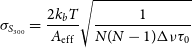 \begin{align} \sigma_{S_{300}} = \frac{2k_bT}{A_{\rm{eff}}}\sqrt{\frac{1}{N(N-1) \Delta\nu \tau_0}}\end{align}
Where  $\tau_0=120$ is the snapshot observation time in seconds,
  $T_{\textrm{sys}} = T_{\textrm{sky}} + T_{Rc}$ the sky temperature at
  $300\,\textrm{MHz}$ summed with the receiver temperature,
  $A_{\textrm{eff}}=4.75\,\textrm{m}^2$ is the effective tile area (Ung Reference Ung2019),
  $N=128$ is the number of tiles,
  $k_b$ is Boltzmann’s constant, and
  $\Delta\nu = 30.72\,\textrm{MHz}$ is the bandwidth. The sky temperature is given by
  $T_{\textrm{sky}} = 60\lambda^{2.25}\,\textrm{K}$ (Tingay et al. Reference Tingay2013), hence at
  $300\,\textrm{MHz}$,
  $T_{\textrm{sky}} = 60\,\textrm{K}$. Finally
  $T_{Rc} = 180\,\textrm{K}$, therefore
  $T_{\textrm{sys}} = 240\,\textrm{K}$. Using these values the sensitivity is estimated to be
  $\sigma_{S_{300}} \approx 19\,\textrm{mJy}$. This is the best case scenario assuming that no fine channels are flagged.
Equation (8) is the estimated RMS for a naturally weighted set of visibilities. In reality there are many kinds of weighting schemes that can be applied to the data, these affect the sensitivity. An in depth derivation of interferometric sensitivity and how weighting schemes can affect the RMS can be found in Section 6.2.3 of (Thompson Reference Thompson2017).
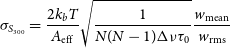 \begin{equation} \sigma_{S_{300}} = \frac{2k_bT}{A_{\textrm{eff}}} \sqrt{\frac{1}{N(N-1)\Delta\nu \tau_0}} \frac{w_{\textrm{mean}}}{w_\textrm{rms}}\end{equation}
Equation (9) represents the general form which accounts for the weighting of the data. The general from is Equation (8) scaled by the ratio of the mean weighting to the RMS of the weightings.
A.1 Sensitivity of flagged data
Following a similar argument we can likewise express  $\sigma^\prime_{S_{300}}$ as:
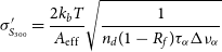 \begin{equation} \sigma^\prime_{S_{300}} = \frac{2k_bT}{A_{\rm{eff}}}\sqrt{\frac{1}{n_d(1-R_f) \tau_\alpha \Delta\nu_\alpha}}\end{equation}
We then have the relationship:
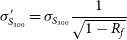 \begin{equation} \sigma^\prime_{S_{300}} = \sigma_{S_{300}}\frac{1}{\sqrt{1-R_f}}\end{equation}
Using Equation (11) if we know the percentage of data flagged we can estimate the expected theoretical sensitivity of the observation. This does not take into consideration the different weighting schemes that are applied to the independent visibility data points.
B. Polylogarithmic coordinate transformation proof
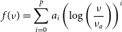 \begin{align} f(\nu) &= \sum^p_{i=0} a_i \left( \log\left( \frac{\nu}{\nu_a}\right)\right)^i \end{align}
 \begin{align} g(\nu) &= \sum^p_{i=0} b_i \left( \log\left( \frac{\nu}{\nu_b}\right)\right)^i\end{align}
In the above equations  $\nu_a$ and
  $\nu_b$ are the normalisation constants for their respective polylogarithmic functions. Now consider the scenario where
  $f(\nu)=g(\nu)\: \forall \: \nu \: \in \: \mathbb{R}$, but
  $\nu_a \neq \nu_b$ and
  $a_i \neq b_i \: \forall \: i$.
Proposition: There should exist a general transform of the coefficients  $a_i$ from the space
  $\nu/\nu_a$ to the space
  $\nu/\nu_b$
There should exist an expression for each coefficient  $b_i$ as a linear combination of the product of the coefficients
  $a_i$,
  $\log(\nu_b/\nu_a)$, and the binomial coefficients:
 \begin{equation} b_l = \sum^p_{i=l} a_i \bigg(\begin{array}{c}
i \\[-3pt]
{i-l}\end{array}\bigg) \left(\log\left( \frac{\nu_b}{\nu_a} \right)\right)^{i-l}\end{equation}
\begin{equation} b_l = \sum^p_{i=l} a_i \bigg(\begin{array}{c}
i \\[-3pt]
{i-l}\end{array}\bigg) \left(\log\left( \frac{\nu_b}{\nu_a} \right)\right)^{i-l}\end{equation}
Proof: Here we will show through induction how to express equation (7) as a linear combination of the terms  $\log(\nu/\nu_b)$ and hence derive an expression for each of the coefficients
  $b_i$. First we let
  $\log(\nu/\nu_a) = \log(\nu/\nu_b) + \log(\nu_b/\nu_a) = x + y$, we can then rewrite equation (7):
 \begin{multline} f(x(\nu)) = \sum^p_{i=0}a_i\left(x + y \right)^i = a_0 + a_1\left(x + y \right) + \cdots +\\ a_{p-1}\left(x+y\right)^{p-1} + a_p \left(x+y\right)^p \end{multline}
We can expand each term in the sum  $\left(x + y\right)^i$ through a binomial expansion, and hence rewrite each
  $\left(x + y \right)^i$ term as a sum:
 \begin{equation}\begin{split}f(x(\nu)) &= \sum^p_{i=0} a_i \left[\bigg(\begin{array}{c}
i \\[-3pt]
0\end{array}\bigg) x^i + {\bigg(\begin{array}{c}
i \\[-3pt]
1\end{array}\bigg)} x^{i-1} y + \cdots \right. \\ &\left.+ {\bigg(\begin{array}{c}
i \\[-3pt]
{i-l}\end{array}\bigg)}xy^{i-1} + {\bigg(\begin{array}{c}
i \\[-3pt]
{i}\end{array}\bigg)} y^i \right] \\ &= \sum^p_{i=0} a_i \sum^i_{j=0} {\bigg(\begin{array}{c}
i \\[-3pt]
j\end{array}\bigg)} x^{i-j}y^j\end{split}\end{equation}
\begin{equation}\begin{split}f(x(\nu)) &= \sum^p_{i=0} a_i \left[\bigg(\begin{array}{c}
i \\[-3pt]
0\end{array}\bigg) x^i + {\bigg(\begin{array}{c}
i \\[-3pt]
1\end{array}\bigg)} x^{i-1} y + \cdots \right. \\ &\left.+ {\bigg(\begin{array}{c}
i \\[-3pt]
{i-l}\end{array}\bigg)}xy^{i-1} + {\bigg(\begin{array}{c}
i \\[-3pt]
{i}\end{array}\bigg)} y^i \right] \\ &= \sum^p_{i=0} a_i \sum^i_{j=0} {\bigg(\begin{array}{c}
i \\[-3pt]
j\end{array}\bigg)} x^{i-j}y^j\end{split}\end{equation}
By factoring out the zeroth x terms we can rewrite the expression in equation (12):
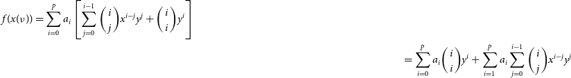 \begin{multline} f(x(\nu)) = \sum^p_{i=0} a_i \left[\sum^{i-1}_{j=0} {\bigg(\begin{array}{c}
i \\[-3pt]
j\end{array}\bigg)} x^{i-j}y^j + {\bigg(\begin{array}{c}
i \\[-3pt]
{i}\end{array}\bigg)} y^i \right]\\ =\sum^p_{i=0} a_i {\bigg(\begin{array}{c}
i \\[-3pt]
{i}\end{array}\bigg)} y^i + \sum^p_{i=1} a_i \sum^{i-1}_{j=0} {\bigg(\begin{array}{c}
i \\[-3pt]
j\end{array}\bigg)} x^{i-j}y^j\end{multline}
\begin{multline} f(x(\nu)) = \sum^p_{i=0} a_i \left[\sum^{i-1}_{j=0} {\bigg(\begin{array}{c}
i \\[-3pt]
j\end{array}\bigg)} x^{i-j}y^j + {\bigg(\begin{array}{c}
i \\[-3pt]
{i}\end{array}\bigg)} y^i \right]\\ =\sum^p_{i=0} a_i {\bigg(\begin{array}{c}
i \\[-3pt]
{i}\end{array}\bigg)} y^i + \sum^p_{i=1} a_i \sum^{i-1}_{j=0} {\bigg(\begin{array}{c}
i \\[-3pt]
j\end{array}\bigg)} x^{i-j}y^j\end{multline}
Since all the zeroth order x terms have been factored out, the new inner sum reduces by 1, and the outer sum subsequently increments by 1 since the inner sum cannot start at  $-1$. This factorisation process can be extended to each successive lowest order x term, to generally prove this, consider the arbitrary step k which is defined below:
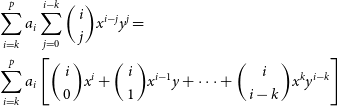 \begin{equation}\begin{split} &\sum^p_{i=k} a_i \sum^{i-k}_{j=0} {\bigg(\begin{array}{c}
i \\[-3pt]
j\end{array}\bigg)} x^{i-j}y^j =\\ &\sum^p_{i=k} a_i \left[ {\bigg(\begin{array}{c}
i \\[-3pt]
0\end{array}\bigg)} x^i + {\bigg(\begin{array}{c}
i \\[-3pt]
1\end{array}\bigg)} x^{i-1} y + \cdots + {\bigg(\begin{array}{c}
i \\[-3pt]
{i-k}\end{array}\bigg)} x^ky^{i-k} \right]\end{split}\end{equation}
\begin{equation}\begin{split} &\sum^p_{i=k} a_i \sum^{i-k}_{j=0} {\bigg(\begin{array}{c}
i \\[-3pt]
j\end{array}\bigg)} x^{i-j}y^j =\\ &\sum^p_{i=k} a_i \left[ {\bigg(\begin{array}{c}
i \\[-3pt]
0\end{array}\bigg)} x^i + {\bigg(\begin{array}{c}
i \\[-3pt]
1\end{array}\bigg)} x^{i-1} y + \cdots + {\bigg(\begin{array}{c}
i \\[-3pt]
{i-k}\end{array}\bigg)} x^ky^{i-k} \right]\end{split}\end{equation}
We see in equation (15) that similar to the form written in equation (11), that if we let  $k=0$ we reduce to the entire sum. Now we factor out the kth order x term from equation (15):
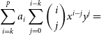 \begin{align} &\sum^p_{i=k} a_i \sum^{i-k}_{j=0} {\bigg(\begin{array}{c}
i \\[-3pt]
j\end{array}\bigg)} x^{i-j}y^j = \end{align}
\begin{align} &\sum^p_{i=k} a_i \sum^{i-k}_{j=0} {\bigg(\begin{array}{c}
i \\[-3pt]
j\end{array}\bigg)} x^{i-j}y^j = \end{align}
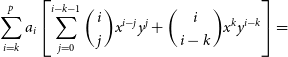 \begin{align} &\sum^p_{i=k} a_i \left[\sum^{i-k-1}_{j=0} {\bigg(\begin{array}{c}
i \\[-3pt]
j\end{array}\bigg)} x^{i-j}y^j + {\bigg(\begin{array}{c}
i \\[-3pt]
{i-k}\end{array}\bigg)} x^ky^{i-k} \right] =\end{align}
\begin{align} &\sum^p_{i=k} a_i \left[\sum^{i-k-1}_{j=0} {\bigg(\begin{array}{c}
i \\[-3pt]
j\end{array}\bigg)} x^{i-j}y^j + {\bigg(\begin{array}{c}
i \\[-3pt]
{i-k}\end{array}\bigg)} x^ky^{i-k} \right] =\end{align}
 \begin{align} &\left( \sum^p_{i=k} a_i {\bigg(\begin{array}{c}
i \\[-3pt]
{i-k}\end{array}\bigg)} y^{i-k} \right)x^k + \sum^p_{i=k+1} a_i \sum^{i-k-1}_{j=0} {\bigg(\begin{array}{c}
i \\[-3pt]
j\end{array}\bigg)} x^{i-j}y^j\end{align}
\begin{align} &\left( \sum^p_{i=k} a_i {\bigg(\begin{array}{c}
i \\[-3pt]
{i-k}\end{array}\bigg)} y^{i-k} \right)x^k + \sum^p_{i=k+1} a_i \sum^{i-k-1}_{j=0} {\bigg(\begin{array}{c}
i \\[-3pt]
j\end{array}\bigg)} x^{i-j}y^j\end{align}
Again we see that this factorisation reflects that of the zeroth order term. If we let  $p=k+1$, hence
  $k=p-1$, then we retrieve the last two terms of the factorisation, for the highest and second highest orders of x:
 \begin{multline} \sum^p_{i=k} a_i \sum^{i-k}_{j=0} {\bigg(\begin{array}{c}
i \\[-3pt]
j\end{array}\bigg)} x^{i-j}y^j =\\ \left( \sum^p_{i=p-1} a_i {
\bigg(\begin{array}{c}
i \\[-3pt]
i-(p-1)\end{array}\bigg)} y^{i-(p-1)} \right)x^{p-1} + a_p \bigg(\begin{array}{c}
p \\[-3pt]
0\end{array}\bigg) x^p \end{multline}
\begin{multline} \sum^p_{i=k} a_i \sum^{i-k}_{j=0} {\bigg(\begin{array}{c}
i \\[-3pt]
j\end{array}\bigg)} x^{i-j}y^j =\\ \left( \sum^p_{i=p-1} a_i {
\bigg(\begin{array}{c}
i \\[-3pt]
i-(p-1)\end{array}\bigg)} y^{i-(p-1)} \right)x^{p-1} + a_p \bigg(\begin{array}{c}
p \\[-3pt]
0\end{array}\bigg) x^p \end{multline}
We are now in a position to express equation (10) as a linear combination of x:
 \begin{align} &f(x(\nu)) = \sum^p_{i=0} a_i {\bigg(\begin{array}{c}
i \\[-3pt]
i\end{array}\bigg)} y^i + \cdots \end{align}
\begin{align} &f(x(\nu)) = \sum^p_{i=0} a_i {\bigg(\begin{array}{c}
i \\[-3pt]
i\end{array}\bigg)} y^i + \cdots \end{align}
 \begin{align} &+ \left( \sum^p_{i=l} a_i {\bigg(\begin{array}{c}
i \\[-3pt]
i-l\end{array}\bigg)} y^{i-l} \right) x^l + \cdots + a_p {\bigg(\begin{array}{c}
p \\[-3pt]
0\end{array}\bigg)} x^p \end{align}
\begin{align} &+ \left( \sum^p_{i=l} a_i {\bigg(\begin{array}{c}
i \\[-3pt]
i-l\end{array}\bigg)} y^{i-l} \right) x^l + \cdots + a_p {\bigg(\begin{array}{c}
p \\[-3pt]
0\end{array}\bigg)} x^p \end{align}
 \begin{align} &= b_0 + \cdots + b_l x^l + \cdots + b_p x^p = g(x(\nu))\end{align}
It is clear to see how the coefficients of  $f(x(\nu))$ map to the coefficients of
  $g(x(\nu))$, specifically the total sum can be expressed as:
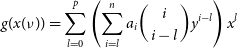 \begin{align} g(x(\nu)) &= \sum^p_{l=0}\left(\sum^n_{i=l} a_i {\bigg(\begin{array}{c}
i \\[-3pt]
i-l\end{array}\bigg)} y^{i-l} \right) x^l \end{align}
\begin{align} g(x(\nu)) &= \sum^p_{l=0}\left(\sum^n_{i=l} a_i {\bigg(\begin{array}{c}
i \\[-3pt]
i-l\end{array}\bigg)} y^{i-l} \right) x^l \end{align}
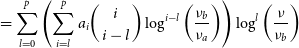 \begin{align} &= \sum^p_{l=0}\left(\sum^p_{i=l} a_i {\bigg(\begin{array}{c}
i \\[-3pt]
i-l\end{array}\bigg)} \log^{i-l}\left(\frac{\nu_b}{\nu_a}\right) \right) \log^l\left(\frac{\nu}{\nu_b}\right)\end{align}
\begin{align} &= \sum^p_{l=0}\left(\sum^p_{i=l} a_i {\bigg(\begin{array}{c}
i \\[-3pt]
i-l\end{array}\bigg)} \log^{i-l}\left(\frac{\nu_b}{\nu_a}\right) \right) \log^l\left(\frac{\nu}{\nu_b}\right)\end{align}
And hence for an arbitrary coefficient  $b_l$ we can express the transformation as:
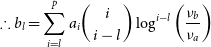 \begin{equation} \therefore b_l = \sum^p_{i=l} a_i {\bigg(\begin{array}{c}
i \\[-3pt]
i-l\end{array}\bigg)} \log^{i-l}\left(\frac{\nu_b}{\nu_a}\right)\end{equation}
\begin{equation} \therefore b_l = \sum^p_{i=l} a_i {\bigg(\begin{array}{c}
i \\[-3pt]
i-l\end{array}\bigg)} \log^{i-l}\left(\frac{\nu_b}{\nu_a}\right)\end{equation}
B.1 Matrix representation of the polylogarithmic coefficient transformation function
We can see the emergent pattern where the sum of binomial coefficients in equation (23) is the linear combination of the right diagonals on pascals triangle, where l is the order.
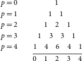 \begin{align*}
p&=0\qquad\qquad\quad\! 1\\
p&=1\qquad\qquad 1\quad 1\\
p&=2\qquad\qquad\!\!\! 1\quad 2\quad 1\\
p&=3\qquad\quad\!\! 1\quad 3\quad 3\quad 1\\
p&=4\qquad 1\quad 4\quad 6\quad 4\quad 1\\[-5pt]
&\qquad\quad\ \ \frac{}{0\quad 1\quad 2\quad 3\quad 4}
\end{align*}
\begin{align*}
p&=0\qquad\qquad\quad\! 1\\
p&=1\qquad\qquad 1\quad 1\\
p&=2\qquad\qquad\!\!\! 1\quad 2\quad 1\\
p&=3\qquad\quad\!\! 1\quad 3\quad 3\quad 1\\
p&=4\qquad 1\quad 4\quad 6\quad 4\quad 1\\[-5pt]
&\qquad\quad\ \ \frac{}{0\quad 1\quad 2\quad 3\quad 4}
\end{align*}
We can use this pattern to define a transformation matrix that will operate on the vector of coefficients:
 \begin{equation*}\textbf{a} =\left(\begin{matrix}a_0 & \quad a_1 & \quad \cdots & \quad a_p\end{matrix}\right)\end{equation*}
Thus transforming vector  $\textbf{a}$ into vector
  $\textbf{b}$:
 \begin{equation*}\textbf{b} =\left(\begin{matrix}b_0 & \quad b_1 & \quad \cdots & \quad b_p\end{matrix}\right)\end{equation*}
Consider the upper triangular matrix  $\textbf{P}_{n,n}$ where the dimensions of the triangular matrix n are defined as the order
  $p+1$, this is equal to the number of coefficients in an arbitrary polynomial.
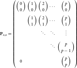 \begin{equation*}\textbf{P}_{n,n} =\left(\begin{matrix}\bigg(\begin{array}{c}
0 \\[-3pt]
0\end{array}\bigg) & \bigg(\begin{array}{c}
1 \\[-3pt]
0\end{array}\bigg) & \bigg(\begin{array}{c}
2 \\[-3pt]
0\end{array}\bigg) & \cdots & \bigg(\begin{array}{c}
p \\[-3pt]
0\end{array}\bigg) \\[5pt] & \bigg(\begin{array}{c}
1 \\[-3pt]
1\end{array}\bigg) & \bigg(\begin{array}{c}
2 \\[-3pt]
1\end{array}\bigg) & \cdots & \bigg(\begin{array}{c}
p \\[-3pt]
1\end{array}\bigg) \\[5pt] & & \ddots & \ddots & \vdots \\[5pt] & & & \ddots & \bigg(\begin{array}{c}
p \\[-3pt]
p-1\end{array}\bigg) \\[5pt]
0 & & & & \bigg(\begin{array}{c}
p \\[-3pt]
p\end{array}\bigg)\end{matrix}\right)\end{equation*}
\begin{equation*}\textbf{P}_{n,n} =\left(\begin{matrix}\bigg(\begin{array}{c}
0 \\[-3pt]
0\end{array}\bigg) & \bigg(\begin{array}{c}
1 \\[-3pt]
0\end{array}\bigg) & \bigg(\begin{array}{c}
2 \\[-3pt]
0\end{array}\bigg) & \cdots & \bigg(\begin{array}{c}
p \\[-3pt]
0\end{array}\bigg) \\[5pt] & \bigg(\begin{array}{c}
1 \\[-3pt]
1\end{array}\bigg) & \bigg(\begin{array}{c}
2 \\[-3pt]
1\end{array}\bigg) & \cdots & \bigg(\begin{array}{c}
p \\[-3pt]
1\end{array}\bigg) \\[5pt] & & \ddots & \ddots & \vdots \\[5pt] & & & \ddots & \bigg(\begin{array}{c}
p \\[-3pt]
p-1\end{array}\bigg) \\[5pt]
0 & & & & \bigg(\begin{array}{c}
p \\[-3pt]
p\end{array}\bigg)\end{matrix}\right)\end{equation*}
Each row in the matrix  $\textbf{P}_{n,n}$ is comprised of the diagonal entries of Pascal’s triangle with order p. The null entries are represented by zeros, and comprise the lower left corner of the upper triangular matrix
  $\textbf{P}_{n,n}$. The next important matrix is the polynomial matrix, which is also an upper triangular matrix, this is represented below:
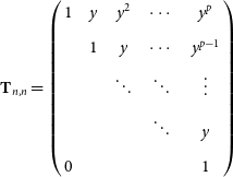 \begin{equation*}\textbf{T}_{n,n} =\left(\begin{array}{c@{\quad}c@{\quad}c@{\quad}c@{\quad}c}1 & y & y^2 & \cdots & y^p \\[3pt]
& 1 & y & \cdots & y^{p-1} \\[3pt]
& & \ddots & \ddots & \vdots \\[3pt]
& & & \ddots & y \\[3pt]
0 & & & & 1\end{array}\right)\end{equation*}
\begin{equation*}\textbf{T}_{n,n} =\left(\begin{array}{c@{\quad}c@{\quad}c@{\quad}c@{\quad}c}1 & y & y^2 & \cdots & y^p \\[3pt]
& 1 & y & \cdots & y^{p-1} \\[3pt]
& & \ddots & \ddots & \vdots \\[3pt]
& & & \ddots & y \\[3pt]
0 & & & & 1\end{array}\right)\end{equation*}
In the matrix  $\textbf{T}_{n,n}$, the variable y takes on the same value as it did in the previous section. The Hadmarad product (element by element product) of the matrices
  $\textbf{P}$ and
  $\textbf{T}$, produces the polylogarithmic coefficient transformation matrix:
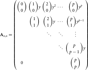 \begin{equation*}\textbf{A}_{n,n} =\left(\begin{matrix}\bigg(\begin{array}{c}
0 \\[-3pt]
0\end{array}\bigg) & \bigg(\begin{array}{c}
1 \\[-3pt]
0\end{array}\bigg)y & \bigg(\begin{array}{c}
2 \\[-3pt]
0\end{array}\bigg)y^2 & \cdots & \bigg(\begin{array}{c}
p \\[-3pt]
0\end{array}\bigg)y^p \\[4pt] & \bigg(\begin{array}{c}
1 \\[-3pt]
1\end{array}\bigg) & \bigg(\begin{array}{c}
2 \\[-3pt]
1\end{array}\bigg)y & \cdots & \bigg(\begin{array}{c}
p \\[-3pt]
1\end{array}\bigg)y^{p-1} \\[4pt] & & \ddots & \ddots & \vdots \\[4pt] & & & \ddots & \bigg(\begin{array}{c}
p \\[-3pt]
p-1\end{array}\bigg)y \\[4pt]
0 & & & & \bigg(\begin{array}{c}
p \\[-3pt]
p\end{array}\bigg)\end{matrix}\right)\end{equation*}
\begin{equation*}\textbf{A}_{n,n} =\left(\begin{matrix}\bigg(\begin{array}{c}
0 \\[-3pt]
0\end{array}\bigg) & \bigg(\begin{array}{c}
1 \\[-3pt]
0\end{array}\bigg)y & \bigg(\begin{array}{c}
2 \\[-3pt]
0\end{array}\bigg)y^2 & \cdots & \bigg(\begin{array}{c}
p \\[-3pt]
0\end{array}\bigg)y^p \\[4pt] & \bigg(\begin{array}{c}
1 \\[-3pt]
1\end{array}\bigg) & \bigg(\begin{array}{c}
2 \\[-3pt]
1\end{array}\bigg)y & \cdots & \bigg(\begin{array}{c}
p \\[-3pt]
1\end{array}\bigg)y^{p-1} \\[4pt] & & \ddots & \ddots & \vdots \\[4pt] & & & \ddots & \bigg(\begin{array}{c}
p \\[-3pt]
p-1\end{array}\bigg)y \\[4pt]
0 & & & & \bigg(\begin{array}{c}
p \\[-3pt]
p\end{array}\bigg)\end{matrix}\right)\end{equation*}
Thus the transformation can be represented by:
 \begin{align} \left(\textbf{P} \circ \textbf{T}\right)\textbf{a}^\top &= \textbf{b}^\top \end{align}
 \begin{align} \therefore \textbf{A}\textbf{a}^\top &= \textbf{b}^\top\end{align}
Example (Second order Polylogarithmic Functions):
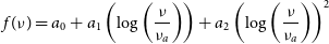 \begin{align} f(\nu) &= a_0 + a_1 \left( \log\left( \frac{\nu}{\nu_a}\right) \right) + a_2 \left( \log\left( \frac{\nu}{\nu_a}\right) \right)^2\end{align}
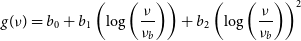 \begin{align} g(\nu) &= b_0 + b_1 \left( \log\left( \frac{\nu}{\nu_b}\right) \right) + b_2 \left( \log\left( \frac{\nu}{\nu_b}\right) \right)^2\end{align}
Hence:
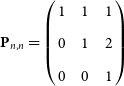 \begin{equation*}\textbf{P}_{n,n} =\left(\begin{array}{c@{\quad}c@{\quad}c} 1 & 1 & 1\\[3pt]
0 & 1 & 2\\[3pt]
0 & 0 & 1\end{array}\right)\end{equation*}
\begin{equation*}\textbf{P}_{n,n} =\left(\begin{array}{c@{\quad}c@{\quad}c} 1 & 1 & 1\\[3pt]
0 & 1 & 2\\[3pt]
0 & 0 & 1\end{array}\right)\end{equation*}
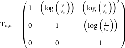 \begin{equation*}\textbf{T}_{n,n} =\left(\begin{array}{c@{\quad}c@{\quad}c} 1 & \left( \log\left( \frac{\nu}{\nu_a}\right) \right) & \left( \log\left( \frac{\nu}{\nu_a}\right) \right)^2\\[5pt]
0 & 1 & \left( \log\left( \frac{\nu}{\nu_a}\right) \right)\\[5pt]
0 & 0 & 1\end{array}\right)\end{equation*}
\begin{equation*}\textbf{T}_{n,n} =\left(\begin{array}{c@{\quad}c@{\quad}c} 1 & \left( \log\left( \frac{\nu}{\nu_a}\right) \right) & \left( \log\left( \frac{\nu}{\nu_a}\right) \right)^2\\[5pt]
0 & 1 & \left( \log\left( \frac{\nu}{\nu_a}\right) \right)\\[5pt]
0 & 0 & 1\end{array}\right)\end{equation*}
Thus the polylogarithmic coefficient transformation matrix is:
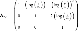 \begin{equation*}\textbf{A}_{n,n} =\left(\begin{array}{c@{\quad}c@{\quad}c} 1 & \left( \log\left( \frac{\nu}{\nu_a}\right) \right) & \left( \log\left( \frac{\nu}{\nu_a}\right) \right)^2\\[6pt]
0 & 1 & 2\left( \log\left( \frac{\nu}{\nu_a}\right) \right)\\[6pt]
0 & 0 & 1\end{array}\right)\end{equation*}
\begin{equation*}\textbf{A}_{n,n} =\left(\begin{array}{c@{\quad}c@{\quad}c} 1 & \left( \log\left( \frac{\nu}{\nu_a}\right) \right) & \left( \log\left( \frac{\nu}{\nu_a}\right) \right)^2\\[6pt]
0 & 1 & 2\left( \log\left( \frac{\nu}{\nu_a}\right) \right)\\[6pt]
0 & 0 & 1\end{array}\right)\end{equation*}
Substituting in the values:
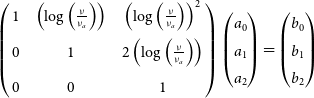 \begin{equation*}\left(\begin{array}{c@{\quad}c@{\quad}c} 1 & \left( \log\left( \frac{\nu}{\nu_a}\right) \right) & \left( \log\left( \frac{\nu}{\nu_a}\right) \right)^2\\[5pt]
0 & 1 & 2\left( \log\left( \frac{\nu}{\nu_a}\right) \right)\\[5pt]
0 & 0 & 1\end{array}\right)\left(\begin{matrix} a_0 \\ a_1 \\ a_2 \\\end{matrix}\right)= \left(\begin{matrix} b_0 \\ b_1 \\ b_2 \\\end{matrix}\right)\end{equation*}
\begin{equation*}\left(\begin{array}{c@{\quad}c@{\quad}c} 1 & \left( \log\left( \frac{\nu}{\nu_a}\right) \right) & \left( \log\left( \frac{\nu}{\nu_a}\right) \right)^2\\[5pt]
0 & 1 & 2\left( \log\left( \frac{\nu}{\nu_a}\right) \right)\\[5pt]
0 & 0 & 1\end{array}\right)\left(\begin{matrix} a_0 \\ a_1 \\ a_2 \\\end{matrix}\right)= \left(\begin{matrix} b_0 \\ b_1 \\ b_2 \\\end{matrix}\right)\end{equation*}
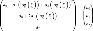 \begin{equation*} \left(\begin{matrix} a_0 + a_1 \left( \log\left( \frac{\nu}{\nu_a}\right) \right) + a_2 \left( \log\left( \frac{\nu}{\nu_a}\right) \right)^2 \\[6pt]
a_0 + 2a_1\left( \log\left( \frac{\nu}{\nu_a}\right) \right) \\[6pt]
a_2 \\\end{matrix}\right)= \left(\begin{matrix} b_0 \\ b_1 \\ b_2 \\\end{matrix}\right)\end{equation*}
\begin{equation*} \left(\begin{matrix} a_0 + a_1 \left( \log\left( \frac{\nu}{\nu_a}\right) \right) + a_2 \left( \log\left( \frac{\nu}{\nu_a}\right) \right)^2 \\[6pt]
a_0 + 2a_1\left( \log\left( \frac{\nu}{\nu_a}\right) \right) \\[6pt]
a_2 \\\end{matrix}\right)= \left(\begin{matrix} b_0 \\ b_1 \\ b_2 \\\end{matrix}\right)\end{equation*}


