


Appendices
Chapter 1 Appendix
CAD code classification for calls for service.
Predatory violent calls: Abduction – other; Aggravated assault; Bank hold up; Carjacking; Common assault; Cutting; Rape (force); Robbery armed; Robbery unarmed; Shooting; Sniper.
Drug calls: Narcotics; Narcotics on-view; Narcotics outside.
Other calls: Abduction by parent; Accident – hit and run; Accident – hit and run pedestrian; Animal cruelty; Animal disturbance; Armed person; Assist officer; Auto theft; Barricade; Bicycle larceny; Bomb scare; Burglary; Cab robbery; Child abuse-physical; Child abuse-sexual; Child neglect; Destruction of Property; Disorderly person; Discharging firearm; Driving while intoxicated; Drug free zone; Family disturbance; False pretense; Gambling; Illegal dumping; Intoxicated person; Investigate auto; Involuntary detention; Juvenile disturbance; Larceny; Larceny from auto; Loud noise; Looting; Mental case; Missing person; Other sex offense; Prostitution complaint; Prowler; Purse snatch; Search & seizure; Special curfew; Stop & frisk; Street disturbance; Street obstruction; Suicide attempt; Suspicious person; Unauthorized use; Vehicle disturbance; Wanted on warrant.
Included types of crime incidents.
Predatory violent crimes: Abduction – other; Aggravated assault; Assault by threat; Bank hold up; Carjacking; Common assault; Cutting, gun, hands or other; Manslaughter; Murder; Rape (attempted); Rape (force); Robbery bank (firearm, knife, other; weapon or unarmed); Robbery carjack – unarmed; Robbery community (firearm, knife, other; weapon or unarmed); Robbery convenience store (firearm, knife, other; weapon or unarmed); Robbery gas station (firearm, knife, other; weapon or unarmed); Robbery highway (firearm, knife, other; weapon or unarmed); Robbery miscellaneous (firearm, knife, other; weapon or unarmed); Robbery residence (firearm, knife, other; weapon or unarmed); Sniper.
Drug crimes: Narcotics; Narcotics civil; Narcotics on-view; Narcotics outside.
Other crimes: Abduction by other; Abduction by parent; Accident – hit and run; Accident – hit and run pedestrian; Animal cruelty; Animal disturbance; Armed person; Assisting prostitution; Barricade; Bomb scare; Burglary; Burglary – other (attempted, no force or with force); Burglary – residential (attempted, no force or with force); Cab robbery; Child abuse-physical; Child abuse-sexual; Child neglect; Destruction of property; Disorderly person; Discharging firearm; Driving while intoxicated; Ex parte; False pretense; Family disturbance; Gambling; Illegal dumping; Intoxicated person; Involuntary detention; Investigate auto; Juvenile disturbance; Larceny – bicycle; Larceny – building; Larceny – from auto; Larceny – from locker; Larceny – machine; Larceny – park meter; Larceny – pickpocket; Larceny – purse snatch; Larceny – shoplifting; Larceny other; Looting; Loud noise; Missing person; Prostitution; Purchasing prostitution; Prowler; Search & seizure; Special curfew; Stolen auto; Stolen bus; Stolen other vehicle; Street disturbance; Suspicious person; Unauthorized use; Vehicle disturbance; Wanted on warrant.
Chapter 2 Appendix
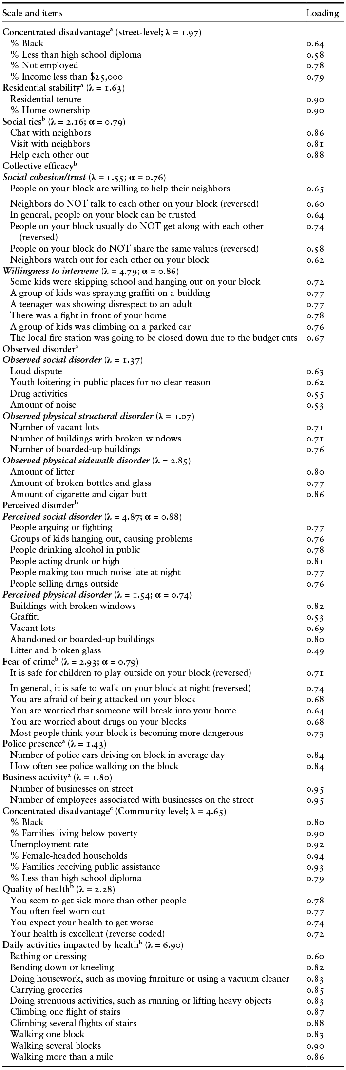
Note:
a = PCA conducted at the street level; b = PCA conducted at the individual level; c = PCA conducted at the community (community statistical area) level.
Chapter 4 Appendix
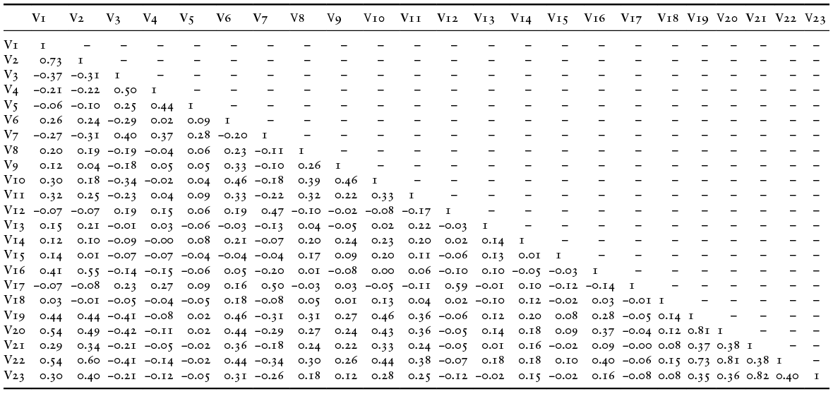
Note: V1 = Citizen crime CFS for 2017; V2 = Crime incident for 2017; V3 = Collective efficacy; V4 = Social ties; V5 = Social network; V6 = Concentrated disadvantage; V7 = Residential stability; V8 = Observed social disorder; V9 = Observed structural physical disorder; V10 = Observed sidewalk physical disorder; V11 = Police presence level; V12 = % Retired; V13 = Business activity; V14 = Bus stops (within ¼ mile); V15 = Bar or liquor store; V16 = Residential street population; V17 = Mean age; V18 = % Female; V19 = Street segment type; V20 = Logged crime CFS for 2012; V21 = Spatial lag for crime CFS for 2017; V22 = Logged crime incident for 2012; V23 = Spatial lag for crime incident for 2017.
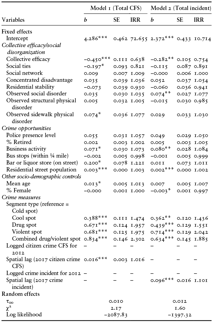
Note: N = 447; SE = standard error; Incidence Rate Ratio (IRR) = exp(b);
* p < 0.05, **p < 0.01, ***p < 0.001.
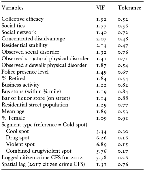
Note: N = 447; VIF = variance inflation factor.
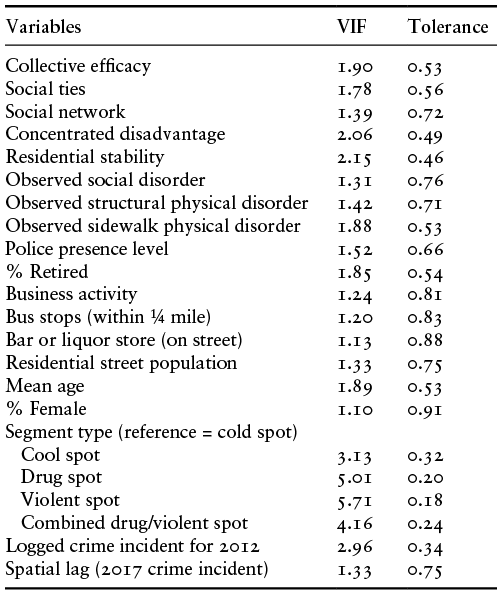
Note: N = 447; VIF = variance inflation factor.
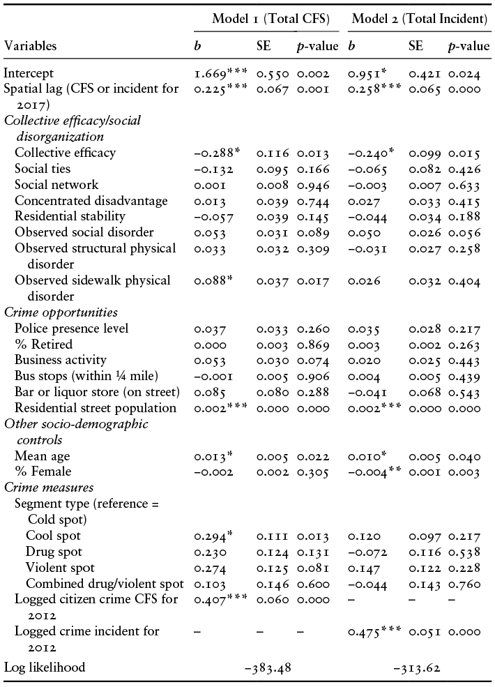
Note: N = 447; SE = standard error;
* p < 0.05, **p < 0.01, ***p < 0.001.
Chapter 5 Appendix
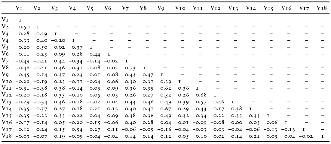
Note: V1 = Collective efficacy at wave 3; V2 = Collective efficacy at wave 1; V3 = Concentrated disadvantage; V4 = Residential stability; V5 = Social ties; V6 = Social network; V7 = Logged crime incident; V8 = Street segment type; V9 = Perceived social disorder; V10 = Observed social disorder; V11 = Perceived physical disorder; V12 = Observed structural physical disorder; V13 = Observed sidewalk physical disorder; V14 = Fear of crime; V15 = Police presence level; V16 = Residential street population; V17 = Mean age; V18 = % Female.
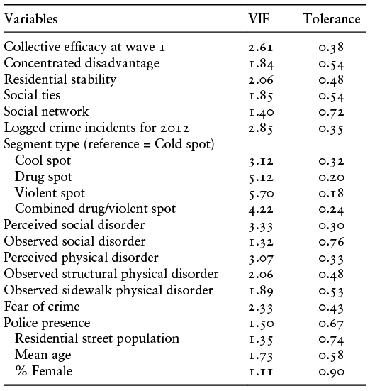
Note: N = 447 VIF = variance inflation factor.
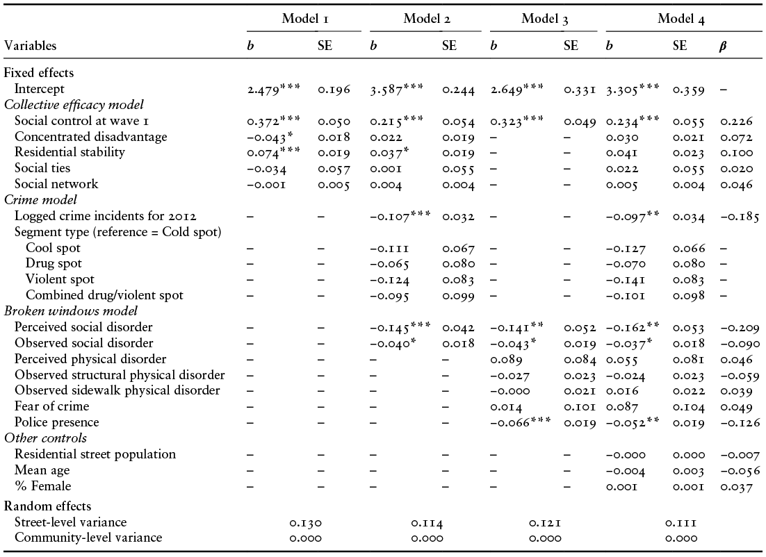
Note: N = 447; SE = standard error;
* p < 0.05, **p < 0.01, ***p < 0.001.
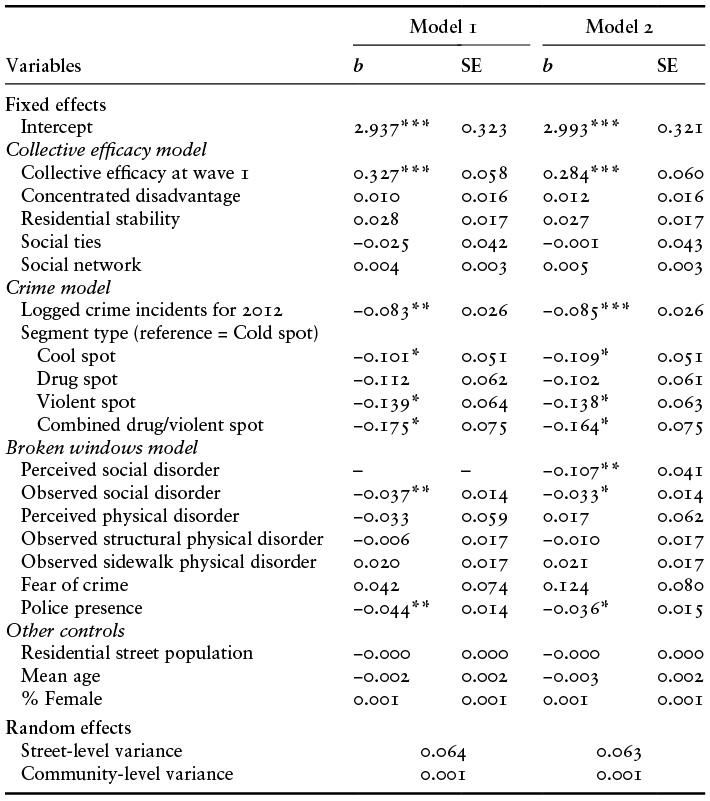
Note: N = 447; SE = standard error;
* p < 0.05, **p < 0.01, ***p < 0.001.
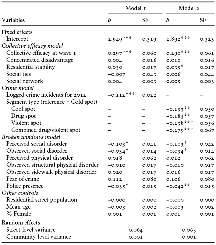
Note: N = 447; SE = standard error;
* p < 0.05, **p < 0.01, ***p < 0.001.
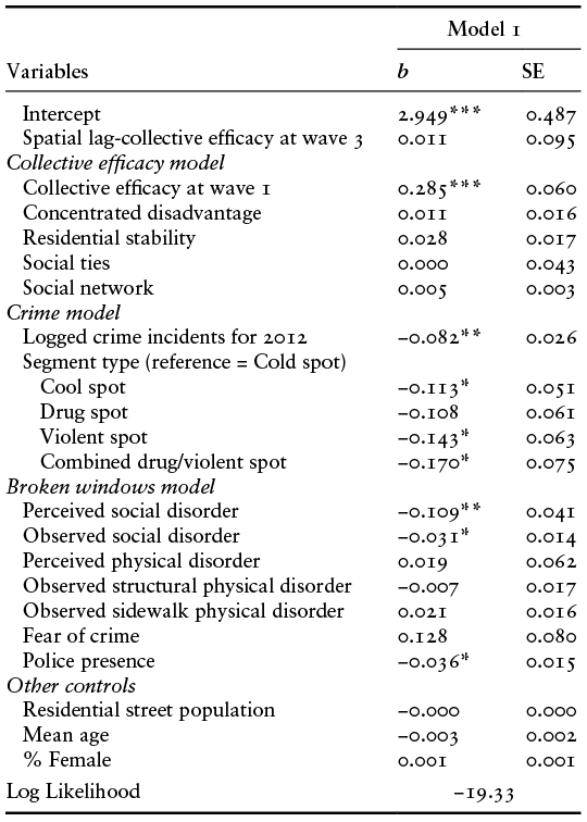
Note: N = 447; SE = standard error;
* p < 0.05, **p < 0.01, ***p < 0.001; Spatial lag is at a distance of 4825.63.
Chapter 6 Appendix

Note: N = 10,438;
*** p < 0.001.
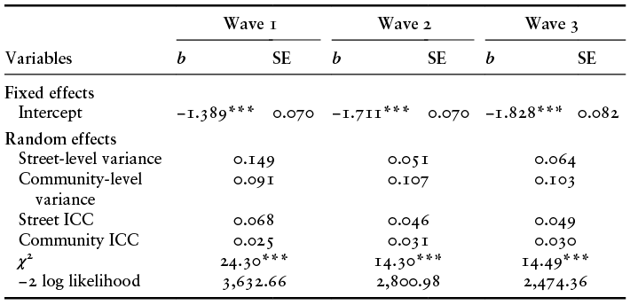
Note:
* p < 0.05, **p < 0.01, ***p < 0.001; Ns are at the individual level and vary between 2,961 and 3,509.
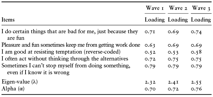
Note: Ns are at the individual level and vary between 2,961 and 3,509.
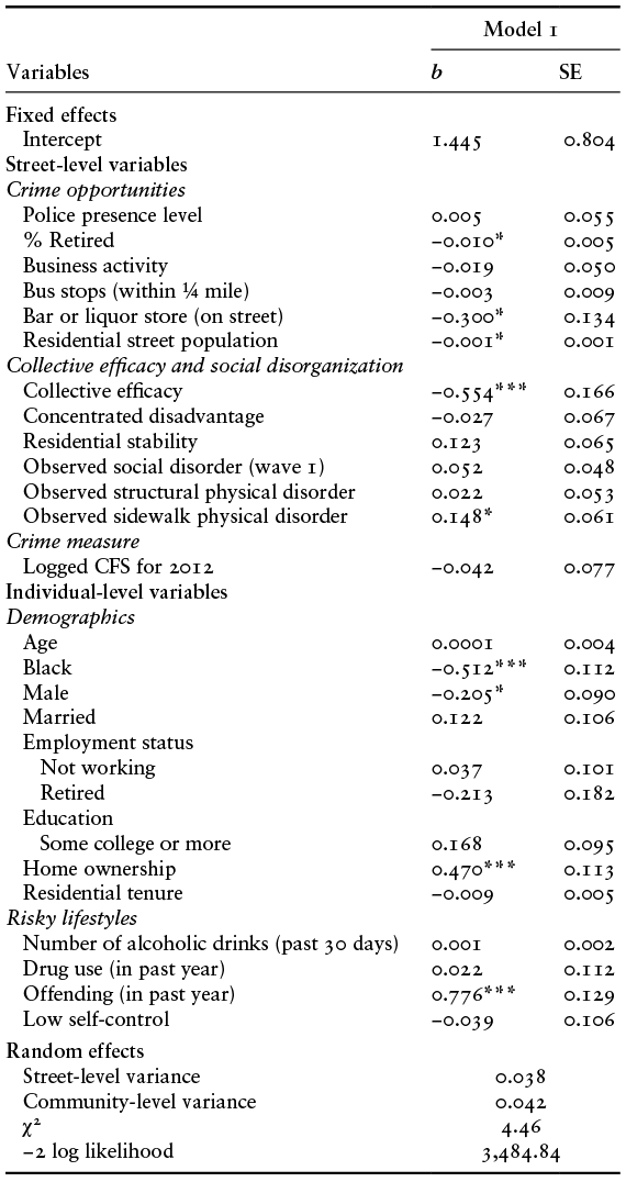
Note: N = 3,509;
* p < 0.05, **p < 0.01, ***p < 0.001; SE = standard error.
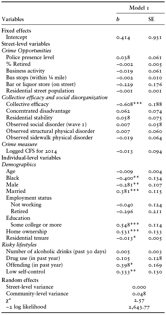
Note: N = 3,204;
* p < 0.05, **p < 0.01, ***p < 0.001; SE = standard error.
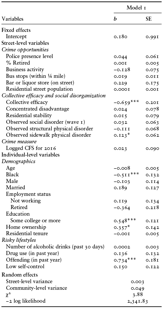
Note: N = 2,961;
* p < 0.05, **p < 0.01, ***p < 0.001; SE = standard error.
Chapter 7 Appendix
Covariates in Propensity Score Analysis
List of the covariates: Being male; Family income less than $10,000; Family income between $10,001 and $25,000; Family income between $25,001 and $40,000; Family income between $40,001 and $60,000; Family income between $60,001 and $80,000; Family income between $80,001 and $100,000; Family income more than $100,000; Currently have a gun in the household; Number of people under 18 live at the address; Being African American; Age of respondents; Working full-time; Working part-time; Not working; Being married; Some middle school or high school education; High school diploma; Some college education; Associate’s degree; Bachelor’s degree; Master’s graduate or professional degree; Low self-control; Self-reported offending behavior; Number of days drink alcohol in average month; Ever used illicit drugs; Number of times arrested in past year; Prosocial values; Reason for moving to block: closer to a job or school; Reason for moving to block: to get away from crime; Reason for moving to block: to have better stores or public services; Reason for moving to block: to get away from drugs; Reason for moving to block: to have better schools for children; Reason for moving to block: for better rent or housing; Reason for moving to block: to move children away from other kids who are a bad influence; Reason for moving to block: to live in a safer neighborhood; Reason for moving to block: to be somewhere with less racial tension; Rent or own home; Length lived on block (months).
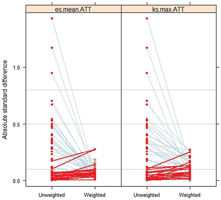
Graphical assessment of balance (wave 1 crime hot spots vs. cold spots)
Note: The effect size plot illustrates the impact of weighting on the magnitude of differences between groups on each pretreatment covariate. The plot shows substantial reductions in effect sizes for most variables after weighting. Closed circles represent statistically significant differences, with many observed before weighting and barely any after weighting.
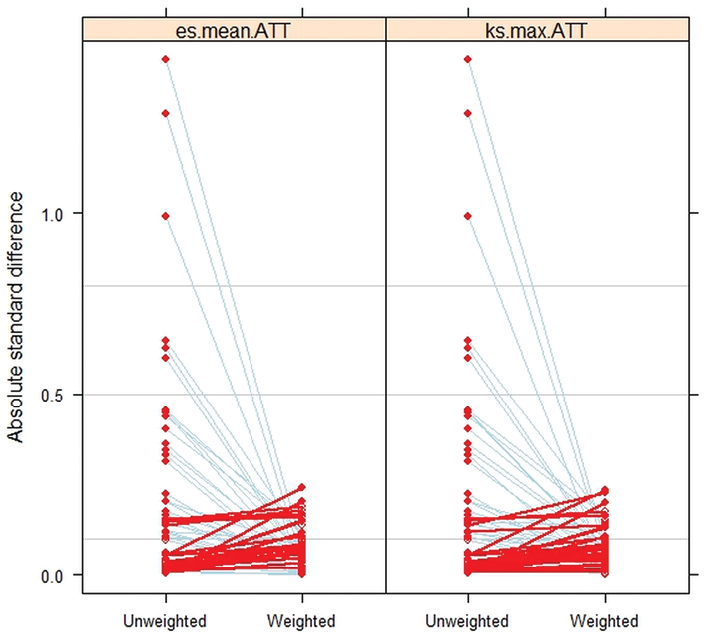
Graphical assessment of balance (wave 2 crime hot spots vs. cold spots)
Note: The effect size plot illustrates the impact of weighting on the magnitude of differences between groups on each pretreatment covariate. The plot shows substantial reductions in effect sizes for most variables after weighting. Closed circles represent statistically significant differences, with many observed before weighting and barely any after weighting.
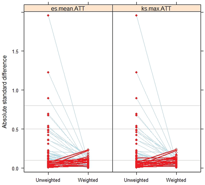
Graphical assessment of balance (wave 3 crime hot spots vs. cold spots)
Note: The effect size plot illustrates the impact of weighting on the magnitude of differences between groups on each pretreatment covariate. The plot shows substantial reductions in effect sizes for most variables after weighting. Closed circles represent statistically significant differences, with many observed before weighting and barely any after weighting.

 Open access