1 INTRODUCTION
Numerical simulations are the ‘third pillar’ of astrophysics, standing alongside observations and analytic theory. Since it is difficult to perform laboratory experiments in the relevant physical regimes and over the correct range of length and timescales involved in most astrophysical problems, we turn instead to ‘numerical experiments’ in the computer for understanding and insight. As algorithms and simulation codes become ever more sophisticated, the public availability of simulation codes has become crucial to ensure that these experiments can be both verified and reproduced.
Phantom is a smoothed particle hydrodynamics (SPH) code developed over the last decade. It has been used widely for studies of turbulence (e.g. Kitsionas et al. Reference Kitsionas2009; Price & Federrath Reference Price and Federrath2010; Price, Federrath, & Brunt Reference Price, Federrath and Brunt2011), accretion (e.g. Lodato & Price Reference Lodato and Price2010; Nixon, King, & Price Reference Nixon, King and Price2012a; Rosotti, Lodato, & Price Reference Rosotti, Lodato and Price2012), star formation including non-ideal magnetohydrodynamics (MHD) (e.g. Wurster et al. Reference Wurster, Price and Bate2016, Wurster, Price, & Bate Reference Wurster, Price and Bate2017), star cluster formation (Liptai et al. Reference Liptai, Price, Wurster and Bate2017), and for studies of the Galaxy (Pettitt et al. Reference Pettitt, Dobbs, Acreman and Price2014; Dobbs et al. Reference Dobbs, Price, Pettitt, Bate and Tricco2016), as well as for simulating dust–gas mixtures (e.g. Dipierro et al. Reference Dipierro, Price, Laibe, Hirsh and Cerioli2015; Ragusa et al. Reference Ragusa, Dipierro, Lodato, Laibe and Price2017; Tricco, Price, & Laibe Reference Tricco, Price and Laibe2017). Although the initial applications and some details of the basic algorithm were described in Price & Federrath (Reference Price and Federrath2010), Lodato & Price (Reference Lodato and Price2010), and Price (Reference Price2012a), the code itself has never been described in detail and, until now, has remained closed source.
One of the initial design goals of Phantom was to have a low memory footprint. A secondary motivation was the need for a public SPH code that is not primarily focused on cosmology, as in the highly successful Gadget code (Springel, Yoshida, & White Reference Springel, Yoshida and White2001; Springel Reference Springel2005). The needs of different communities produce rather different outcomes in the code. For cosmology, the main focus is on simulating the gravitational collapse of dark matter in large volumes of the universe, with gas having only a secondary effect. This is reflected in the ability of the public Gadget-2 code to scale to exceedingly large numbers of dark matter particles, yet neglecting elements of the core SPH algorithm that are essential for stellar and planetary problems, such as the Morris & Monaghan (Reference Morris and Monaghan1997) artificial viscosity switch [c.f. the debate between Bauer & Springel (Reference Bauer and Springel2012) and Price (Reference Price2012b)], the ability to use a spatially variable gravitational force softening (Bate & Burkert Reference Bate and Burkert1997; Price & Monaghan Reference Price and Monaghan2007) or any kind of artificial conductivity, necessary for the correct treatment of contact discontinuities (Chow & Monaghan Reference Chow and Monaghan1997; Price & Monaghan Reference Price and Monaghan2005; Rosswog & Price Reference Rosswog and Price2007; Price Reference Price2008). Almost all of these have since been implemented in development versions of Gadget-3 (e.g. Iannuzzi & Dolag Reference Iannuzzi and Dolag2011; Beck et al. Reference Beck2016; see recent comparison project by Sembolini et al. Reference Sembolini2016) but remain unavailable or unused in the public version. Likewise, the implementation of dust, non-ideal MHD, and other physics relevant to star and planet formation is unlikely to be high priority in a code designed for studying cosmology or galaxy formation.
Similarly, the sphng code (Benz et al. Reference Benz, Cameron, Press and Bowers1990; Bate Reference Bate1995) has been a workhorse for our group for simulations of star formation (e.g. Price & Bate Reference Price and Bate2007, Reference Price and Bate2009; Price, Tricco, & Bate Reference Price, Tricco and Bate2012; Lewis, Bate, & Price Reference Lewis, Bate and Price2015) and accretion discs (e.g. Lodato & Rice Reference Lodato and Rice2004; Cossins, Lodato, & Clarke Reference Cossins, Lodato and Clarke2009), contains a rich array of physics necessary for star and planet formation including all of the above algorithms, but the legacy nature of the code makes it difficult to modify or debug and there are no plans to make it public.
Gasoline (Wadsley, Stadel, & Quinn Reference Wadsley, Stadel and Quinn2004) is another code that has been widely and successfully used for galaxy formation simulations, with its successor, Gasoline 2 (Wadsley et al. Reference Wadsley, Keller and Quinn2017), recently publicly released. Hubber et al. (Reference Hubber, Batty, McLeod and Whitworth2011) have developed Seren with similar goals to Phantom, focused on star cluster simulations. Seren thus presents more advanced N-body algorithms compared to what is in Phantom but does not yet include magnetic fields, dust, or H2 chemistry.
A third motivation was the need to distinguish between the ‘high performance’ code used for 3D simulations from simpler codes used to develop and test algorithms, such as our already-public ndspmhd code (Price Reference Price2012a). Phantom is designed to ‘take what works and make it fast’, rather than containing options for every possible variation on the SPH algorithm. Obsolete options are actively deleted.
The initial release of Phantom has been developed with a focus on stellar, planetary, and Galactic astrophysics, as well as accretion discs. In this first paper, coinciding with the first stable public release, we describe and validate the core algorithms as well as some example applications. Various novel aspects and optimisation strategies are also presented. This paper is an attempt to document in detail what is currently available in the code, which include modules for MHD, dust–gas mixtures, self-gravity, and a range of other physics. The paper is also designed to serve as guide to the correct use of the various algorithms. Stable releases of Phantom are posted on the webFootnote 1, while the development version and wiki documentation are available on the Bitbucket platformFootnote 2.
The paper is organised as follows: We describe the numerical methods in Section 2 with corresponding numerical tests in Section 5. We cover SPH basics (Section 2.1), our implementation of hydrodynamics (Sections 2.2 and 5.1), the timestepping algorithm (Section 2.3), external forces (Sections 2.4 and 5.2), turbulent forcing (Sections 2.5 and 6.1), accretion disc viscosity (Sections 2.6 and 5.3), Navier–Stokes viscosity (Sections 2.7 and 5.4), sink particles (Sections 2.8 and 5.5), stellar physics (Section 2.9), MHD (Sections 2.10 and 5.6), non-ideal MHD (Sections 2.11 and 5.7), self-gravity (Sections 2.12 and 5.8), dust–gas mixtures (Sections 2.13 and 5.9), ISM chemistry and cooling (Sections 2.14 and 5.10), and particle injection (Section 2.15). We present the algorithms for generating initial conditions in Section 3. Our approach to software engineering is described in Section 4. We give five examples of recent applications highlighting different aspects of Phantom in Section 6. We summarise in Section 7.
2 NUMERICAL METHOD
Phantom is based on the SPH technique, invented by Lucy (Reference Lucy1977) and Gingold & Monaghan (Reference Gingold and Monaghan1977) and the subject of numerous reviews (Benz Reference Benz and Buchler1990; Monaghan Reference Monaghan1992, Reference Monaghan2005, Reference Monaghan2012; Rosswog Reference Rosswog2009; Springel Reference Springel2010; Price Reference Price2012a).
In the following, we adopt the convention that a, b, and c refer to particle indices; i, j, and k refer to vector or tensor indices; and n and m refer to indexing of nodes in the treecode.
2.1. Fundamentals
2.1.1. Lagrangian hydrodynamics
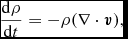
SPH solves the equations of hydrodynamics in Lagrangian form. The fluid is discretised onto a set of ‘particles’ of mass m that are moved with the local fluid velocity  ${\bm v}$. Hence, the two basic equations common to all physics in Phantom are
 \begin{align}
\frac{{\rm d}{\bm r}}{{\rm d}t} = {\bm v},
\end{align}
\begin{align}
\frac{{\rm d}{\bm r}}{{\rm d}t} = {\bm v},
\end{align}
 \begin{align}
\frac{{\rm d}\rho }{{\rm d}t} = -\rho (\nabla \cdot {\bm v}),
\end{align}
\begin{align}
\frac{{\rm d}\rho }{{\rm d}t} = -\rho (\nabla \cdot {\bm v}),
\end{align}
where  ${\bm r}$ is the particle position and ρ is the density. These equations use the Lagrangian time derivative, ${\rm d}/{\rm d}t \equiv \partial / \partial t + {\bm v} \cdot \nabla$, and are the Lagrangian update of the particle position and the continuity equation (expressing the conservation of mass), respectively.
2.1.2. Conservation of mass in SPH
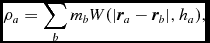
The density is computed in Phantom using the usual SPH density sum
 $$\begin{equation}
\rho _{a} = \sum _{b} m_{b} W(\vert {\bm r}_{a} - {\bm r}_{b}\vert , h_{a}),
\end{equation}$$
$$\begin{equation}
\rho _{a} = \sum _{b} m_{b} W(\vert {\bm r}_{a} - {\bm r}_{b}\vert , h_{a}),
\end{equation}$$
where a and b are particle labels, m is the mass of the particle, W is the smoothing kernel, h is the smoothing length, and the sum is over neighbouring particles (i.e. those within R kernh, where R kern is the dimensionless cut-off radius of the smoothing kernel). Taking the Lagrangian time derivative of (3), one obtains the discrete form of (2) in SPH
 $$\begin{equation}
\frac{{\rm d}\rho _{a}}{{\rm d}t} = \frac{1}{\Omega _{a}} \sum _{b} m_{b} ({\bm v}_{a} - {\bm v}_{b}) \cdot \nabla _{a} W_{ab} (h_{a}),
\end{equation}$$
$$\begin{equation}
\frac{{\rm d}\rho _{a}}{{\rm d}t} = \frac{1}{\Omega _{a}} \sum _{b} m_{b} ({\bm v}_{a} - {\bm v}_{b}) \cdot \nabla _{a} W_{ab} (h_{a}),
\end{equation}$$
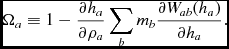
where  $W_{ab}(h_{a})\equiv W(\vert {\bm r}_{a} - {\bm r}_{b}\vert , h_{a})$ and Ωa is a term related to the gradient of the smoothing length (Springel & Hernquist Reference Springel and Hernquist2002; Monaghan Reference Monaghan2002) given by
 $$\begin{equation}
\Omega _{a} \equiv 1 - \frac{\partial h_{a}}{\partial \rho _{a}}\sum _{b} m_{b} \frac{\partial W_{ab} (h_{a})}{\partial h_{a}}.
\end{equation}$$
$$\begin{equation}
\Omega _{a} \equiv 1 - \frac{\partial h_{a}}{\partial \rho _{a}}\sum _{b} m_{b} \frac{\partial W_{ab} (h_{a})}{\partial h_{a}}.
\end{equation}$$
Equation (4) is not used directly to compute the density in Phantom, since evaluating (3) provides a time-independent solution to (2) (see e.g. Monaghan Reference Monaghan1992; Price Reference Price2012a for details). The time-dependent version (4) is equivalent to (3) up to a boundary term (see Price Reference Price2008) but is only used in Phantom to predict the smoothing length at the next timestep in order to reduce the number of iterations required to evaluate the density (see below).
Since (3)–(5) all depend on the kernel evaluated on neighbours within R kern times h a, all three of these summations may be computed simultaneously using a single loop over the same set of neighbours. Details of the neighbour finding procedure are given in Section 2.1.7.
2.1.3. Setting the smoothing length
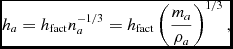
The smoothing length itself is specified as a function of the particle number density, n, via
 $$\begin{equation}
h_{a} = h_{\rm fact} n_{a}^{-1/3} = h_{\rm fact} \left( \frac{m_{a}}{\rho _{a}} \right)^{1/3},
\end{equation}$$
$$\begin{equation}
h_{a} = h_{\rm fact} n_{a}^{-1/3} = h_{\rm fact} \left( \frac{m_{a}}{\rho _{a}} \right)^{1/3},
\end{equation}$$
where h fact is the proportionality factor specifying the smoothing length in terms of the mean local particle spacing and the second equality holds only for equal mass particles, which are enforced in Phantom. The restriction to equal mass particles means that the resolution strictly follows mass, which may be restrictive for problems involving large density contrasts (e.g. Hutchison et al. Reference Hutchison, Price, Laibe and Maddison2016). However, our view is that the potential pitfalls of unequal mass particles (see e.g. Monaghan & Price Reference Monaghan and Price2006) are currently too great to allow for a robust implementation in a public code.
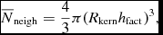
As described in Price (Reference Price2012a), the proportionality constant h fact can be related to the mean neighbour number according to
 $$\begin{equation}
\overline{N}_{\rm neigh} = \frac{4}{3} \pi (R_{\rm kern} h_{\rm fact})^{3},
\end{equation}$$
$$\begin{equation}
\overline{N}_{\rm neigh} = \frac{4}{3} \pi (R_{\rm kern} h_{\rm fact})^{3},
\end{equation}$$
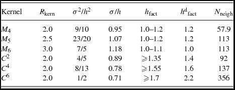
however, this is only equal to the actual neighbour number for particles in a uniform density distribution (more specifically, for a density distribution with no second derivative), meaning that the actual neighbour number varies. The default setting for h fact is 1.2, corresponding to an average of 57.9 neighbours for a kernel truncated at 2h (i.e. for R kern = 2) in three dimensions. Table 1 lists the settings recommended for different choices of kernel. The derivative required in (5) is given by
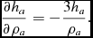 $$\begin{equation}
\frac{\partial h_{a}}{\partial \rho _{a}} = -\frac{3 h_{a}}{\rho _{a}}.
\end{equation}$$
$$\begin{equation}
\frac{\partial h_{a}}{\partial \rho _{a}} = -\frac{3 h_{a}}{\rho _{a}}.
\end{equation}$$
Compact support radii, variance, standard deviation, recommended ranges of h fact, and recommended default h fact settings (hd fact) for the kernel functions available in Phantom.
2.1.4. Iterations for h and ρ
The mutual dependence of ρ and h means that a rootfinding procedure is necessary to solve both (3) and (6) simultaneously. The procedure implemented in Phantom follows Price & Monaghan (Reference Price and Monaghan2004b, Reference Price and Monaghan2007), solving, for each particle, the equation
 $$\begin{equation}
f(h_{a}) = \rho _{\rm sum} (h_{a}) - \rho (h_{a}) = 0,
\end{equation}$$
$$\begin{equation}
f(h_{a}) = \rho _{\rm sum} (h_{a}) - \rho (h_{a}) = 0,
\end{equation}$$
where ρsum is the density computed from (3) and
 $$\begin{equation}
\rho (h_{a}) = m_{a} (h_{\rm fact}/h_{a})^{3},
\end{equation}$$
$$\begin{equation}
\rho (h_{a}) = m_{a} (h_{\rm fact}/h_{a})^{3},
\end{equation}$$
from (6). Equation (9) is solved with Newton–Raphson iterations:
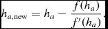 $$\begin{equation}
h_{a, {\rm new}} = h_{a} - \frac{f(h_{a})}{f^{\prime }(h_{a})},
\end{equation}$$
$$\begin{equation}
h_{a, {\rm new}} = h_{a} - \frac{f(h_{a})}{f^{\prime }(h_{a})},
\end{equation}$$
where the derivative is given by
 \begin{align}
f^{\prime }(h_{a}) = \sum _{b} m_{b} \frac{\partial W_{ab} (h_{a})}{\partial h_{a}} - \frac{\partial \rho _{a}}{\partial h_{a}} = -\frac{3\rho _{a}}{h_{a}} \Omega _{a}.
\end{align}
\begin{align}
f^{\prime }(h_{a}) = \sum _{b} m_{b} \frac{\partial W_{ab} (h_{a})}{\partial h_{a}} - \frac{\partial \rho _{a}}{\partial h_{a}} = -\frac{3\rho _{a}}{h_{a}} \Omega _{a}.
\end{align}
The iterations proceed until |h a, new − h a|/h a, 0 < εh, where h a, 0 is the smoothing length of particle a at the start of the iteration procedure and εh is the tolerance. The convergence with Newton–Raphson is fast, with a quadratic reduction in the error at each iteration, meaning that no more than 2–3 iterations are required even with a rapidly changing density field. We avoid further iterations by predicting the smoothing length from the previous timestep according to
 $$\begin{equation}
h^{0}_{a} = h_{a} + \Delta t \frac{{\rm d}h_{a}}{{\rm d}t} = h_{a} + \Delta t \frac{\partial h_{a}}{\partial \rho _{a}} \frac{{\rm d}\rho _{a}}{{\rm d} t},
\end{equation}$$
$$\begin{equation}
h^{0}_{a} = h_{a} + \Delta t \frac{{\rm d}h_{a}}{{\rm d}t} = h_{a} + \Delta t \frac{\partial h_{a}}{\partial \rho _{a}} \frac{{\rm d}\rho _{a}}{{\rm d} t},
\end{equation}$$
where dρa/dt is evaluated from (4).
Since h and ρ are mutually dependent, we store only the smoothing length, from which the density can be obtained at any time via a function call evaluating ρ(h). The default value of εh is 10−4 so that h and ρ can be used interchangeably. Setting a small tolerance does not significantly change the computational cost, as the iterations quickly fall below a tolerance of ‘one neighbour’ according to (7), so any iterations beyond this refer to loops over the same set of neighbours which can be efficiently cached. However, it is important that the tolerance may be enforced to arbitrary precision rather than being an integer as implemented in the public version of Gadget, since (9) expresses a mathematical relationship between h and ρ that is assumed throughout the derivation of the SPH algorithm (see discussion in Price Reference Price2012a). The precision to which this is enforced places a lower limit on the total energy conservation. Fortunately, floating point neighbour numbers are now default in most Gadget-3 variants also.
2.1.5. Kernel functions
We write the kernel function in the form
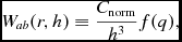 $$\begin{equation}
W_{ab}(r,h) \equiv \frac{C_{\rm norm}}{h^{3}} f(q),
\end{equation}$$
$$\begin{equation}
W_{ab}(r,h) \equiv \frac{C_{\rm norm}}{h^{3}} f(q),
\end{equation}$$
where C norm is a normalisation constant, the factor of h 3 gives the dimensions of inverse volume, and f(q) is a dimensionless function of  $q \equiv \vert {\bm r}_{a} - {\bm r}_{b} \vert / h$. Various relations for kernels in this form are given in Morris (Reference Morris1996a) and in Appendix B of Price (Reference Price2010). Those used in Phantom are the kernel gradient
 $$\begin{equation}
\nabla _{a} W_{ab} = \hat{\bm r}_{ab} F_{ab},\textrm { where } F_{ab} \equiv \frac{C_{\rm norm}}{h^{4}} f^{\prime }(q),
\end{equation}$$
$$\begin{equation}
\nabla _{a} W_{ab} = \hat{\bm r}_{ab} F_{ab},\textrm { where } F_{ab} \equiv \frac{C_{\rm norm}}{h^{4}} f^{\prime }(q),
\end{equation}$$
and the derivative of the kernel with respect to h,
 $$\begin{equation}
\frac{\partial W_{ab}(r,h)}{\partial h} = - \frac{C_{\rm norm}}{h^{4}} \left[ 3 f(q) + qf^{\prime }(q) \right].
\end{equation}$$
$$\begin{equation}
\frac{\partial W_{ab}(r,h)}{\partial h} = - \frac{C_{\rm norm}}{h^{4}} \left[ 3 f(q) + qf^{\prime }(q) \right].
\end{equation}$$
Notice that the ∂W/∂h term in particular can be evaluated simply from the functions needed to compute the density and kernel gradient and hence does not need to be derived separately if a different kernel is used.
2.1.6. Choice of smoothing kernel
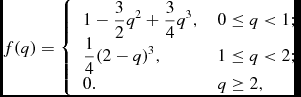
The default kernel function in SPH for the last 30 yr (since Monaghan & Lattanzio Reference Monaghan and Lattanzio1985) has been the M 4 cubic spline from the Schoenberg (Reference Schoenberg1946) B-spline family, given by
 $$\begin{equation}
f(q) = \left\lbrace \arraycolsep5pt\begin{array}{ll}1 - \displaystyle\frac{3}{2} q^{2} + \displaystyle\frac{3}{4} q^{3}, & 0 \le q < 1; \\[3pt]
\displaystyle\frac{1}{4}(2-q)^3, & 1 \le q < 2; \\[3pt]
0. & q \ge 2, \end{array} \right.
\end{equation}$$
$$\begin{equation}
f(q) = \left\lbrace \arraycolsep5pt\begin{array}{ll}1 - \displaystyle\frac{3}{2} q^{2} + \displaystyle\frac{3}{4} q^{3}, & 0 \le q < 1; \\[3pt]
\displaystyle\frac{1}{4}(2-q)^3, & 1 \le q < 2; \\[3pt]
0. & q \ge 2, \end{array} \right.
\end{equation}$$
where the normalisation constant C norm = 1/π in 3D and the compact support of the function implies that R kern = 2. While the cubic spline kernel is satisfactory for many applications, it is not always the best choice. Most SPH kernels are based on approximating the Gaussian, but with compact support to avoid the  $\mathcal {O}(N^{2})$ computational cost. Convergence in SPH is guaranteed to be second order (∝h 2) to the degree that the finite summations over neighbouring particles approximate integrals (e.g. Monaghan Reference Monaghan1992, Reference Monaghan2005; Price Reference Price2012a). Hence, the choice of kernel and the effect that a given kernel has on the particle distribution are important considerations.
In general, more accurate results will be obtained with a kernel with a larger compact support radius, since it will better approximate the Gaussian which has excellent convergence and stability properties (Morris Reference Morris1996a; Price Reference Price2012a; Dehnen & Aly Reference Dehnen and Aly2012). However, care is required. One should not simply increase h fact for the cubic spline kernel because even though this implies more neighbours [via (7)], it increases the resolution length. For the B-splines, it also leads to the onset of the ‘pairing instability’ where the particle distribution becomes unstable to transverse modes, leading to particles forming close pairs (Thomas & Couchman Reference Thomas and Couchman1992; Morris Reference Morris1996a, Reference Morris1996b; Børve, Omang, & Trulsen Reference Børve, Omang and Trulsen2004; Price Reference Price2012a; Dehnen & Aly Reference Dehnen and Aly2012). This is the motivation of our default choice of h fact = 1.2 for the cubic spline kernel, since it is just short of the maximum neighbour number that can be used while remaining stable to the pairing instability.
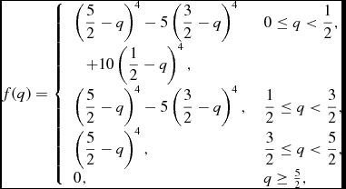
A better approach to reducing kernel bias is to keep the same resolution lengthFootnote 3 but to use a kernel that has a larger compact support radius. The traditional approach (e.g. Morris Reference Morris1996a, Reference Morris1996b; Børve et al. Reference Børve, Omang and Trulsen2004; Price Reference Price2012a) has been to use the higher kernels in the B-spline series, i.e. the M 5 quartic which extends to 2.5h
 $$\begin{equation}
f(q) = \left\lbrace \arraycolsep5pt\begin{array}{ll}
\left(\displaystyle\frac{5}{2} -q\right)^4 - 5\left(\displaystyle\frac{3}{2} -q\right)^4 & 0 \le q < \displaystyle\frac{1}{2}, \\[6pt]
\quad + 10\left(\displaystyle\frac{1}{2}-q\right)^4,\\[6pt]
\left(\displaystyle\frac{5}{2} -q\right)^4 - 5\left(\displaystyle\frac{3}{2} -q\right)^4, & \displaystyle\frac{1}{2} \le q < \displaystyle\frac{3}{2}, \\[6pt]
\left(\displaystyle\frac{5}{2} -q\right)^4, & \displaystyle\frac{3}{2} \le q < \displaystyle\frac{5}{2}, \\[3pt]
0, & q \ge \frac{5}{2}, \end{array} \right.
\end{equation}$$
$$\begin{equation}
f(q) = \left\lbrace \arraycolsep5pt\begin{array}{ll}
\left(\displaystyle\frac{5}{2} -q\right)^4 - 5\left(\displaystyle\frac{3}{2} -q\right)^4 & 0 \le q < \displaystyle\frac{1}{2}, \\[6pt]
\quad + 10\left(\displaystyle\frac{1}{2}-q\right)^4,\\[6pt]
\left(\displaystyle\frac{5}{2} -q\right)^4 - 5\left(\displaystyle\frac{3}{2} -q\right)^4, & \displaystyle\frac{1}{2} \le q < \displaystyle\frac{3}{2}, \\[6pt]
\left(\displaystyle\frac{5}{2} -q\right)^4, & \displaystyle\frac{3}{2} \le q < \displaystyle\frac{5}{2}, \\[3pt]
0, & q \ge \frac{5}{2}, \end{array} \right.
\end{equation}$$
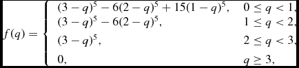
where C norm = 1/(20π), and the M 6 quintic extending to 3h,
 $$\begin{equation}
f(q) = \left\lbrace \arraycolsep5pt\begin{array}{ll}(3-q)^5 - 6(2-q)^5 + 15(1-q)^5, & 0 \le q < 1, \\
(3-q)^5 - 6(2-q)^5, & 1 \le q < 2, \\[3pt]
(3-q)^5, & 2 \le q < 3, \\[3pt]
0, & q \ge 3, \end{array} \right.
\end{equation}$$
$$\begin{equation}
f(q) = \left\lbrace \arraycolsep5pt\begin{array}{ll}(3-q)^5 - 6(2-q)^5 + 15(1-q)^5, & 0 \le q < 1, \\
(3-q)^5 - 6(2-q)^5, & 1 \le q < 2, \\[3pt]
(3-q)^5, & 2 \le q < 3, \\[3pt]
0, & q \ge 3, \end{array} \right.
\end{equation}$$
where C norm = 1/(120π) in 3D. The quintic in particular gives results virtually indistinguishable from the Gaussian for most problems.
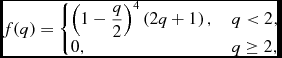
Recently, there has been tremendous interest in the use of the Wendland (Reference Wendland1995) kernels, particularly since Dehnen & Aly (Reference Dehnen and Aly2012) showed that they are stable to the pairing instability at all neighbour numbers despite having a Gaussian-like shape and compact support. These functions are constructed as the unique polynomial functions with compact support but with a positive Fourier transform, which turns out to be a necessary condition for stability against the pairing instability (Dehnen & Aly Reference Dehnen and Aly2012). The 3D Wendland kernels scaled to a radius of 2h are given by C 2:
 $$\begin{equation}
f(q) = \left\lbrace \arraycolsep5pt\begin{array}{@{}ll@{}}\left(1 - \displaystyle\frac{q}{2} \right)^{4} \left(2 q + 1\right), & q < 2, \\[3pt]
0, & q \ge 2, \end{array}\right.
\end{equation}$$
$$\begin{equation}
f(q) = \left\lbrace \arraycolsep5pt\begin{array}{@{}ll@{}}\left(1 - \displaystyle\frac{q}{2} \right)^{4} \left(2 q + 1\right), & q < 2, \\[3pt]
0, & q \ge 2, \end{array}\right.
\end{equation}$$
where C norm = 21/(16π), the C 4 kernel
 $$\begin{equation}
f(q) = \left\lbrace \arraycolsep5pt\begin{array}{@{}ll@{}}\left(1 - \displaystyle\frac{q}{2}\right)^{6} \left(\displaystyle\frac{35 q^{2}}{12} + 3 q + 1\right), & q < 2, \\[3pt]
0, & q\ge 2, \end{array}\right.
\end{equation}$$
$$\begin{equation}
f(q) = \left\lbrace \arraycolsep5pt\begin{array}{@{}ll@{}}\left(1 - \displaystyle\frac{q}{2}\right)^{6} \left(\displaystyle\frac{35 q^{2}}{12} + 3 q + 1\right), & q < 2, \\[3pt]
0, & q\ge 2, \end{array}\right.
\end{equation}$$
where C norm = 495/(256π), and the C 6 kernel
 $$\begin{equation}
f(q) = \left\lbrace \arraycolsep5pt\begin{array}{@{}ll@{}}\left(1 - \displaystyle\frac{q}{2}\right)^{8} \left(4 q^{3} + \displaystyle\frac{25 q^{2}}{4} + 4 q + 1\right), & q < 2, \\[3pt]
0, & q \ge 2, \end{array}\right.
\end{equation}$$
$$\begin{equation}
f(q) = \left\lbrace \arraycolsep5pt\begin{array}{@{}ll@{}}\left(1 - \displaystyle\frac{q}{2}\right)^{8} \left(4 q^{3} + \displaystyle\frac{25 q^{2}}{4} + 4 q + 1\right), & q < 2, \\[3pt]
0, & q \ge 2, \end{array}\right.
\end{equation}$$
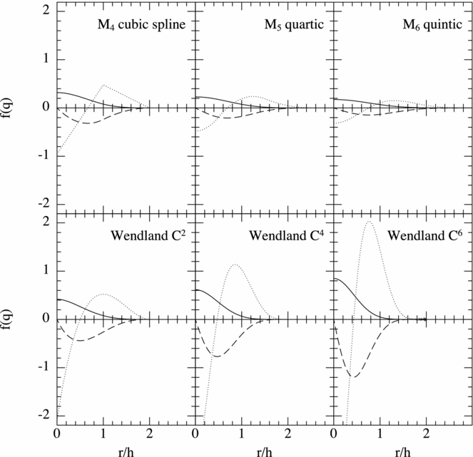
where C norm = 1365/(512π). Figure 1 graphs f(q) and its first and second derivative for each of the kernels available in Phantom.
Smoothing kernels available in Phantom (solid lines) together with their first (dashed lines) and second (dotted lines) derivatives. Wendland kernels in Phantom (bottom row) are given compact support radii of 2, whereas the B-spline kernels (top row) adopt the traditional practice where the support radius increases by 0.5. Thus, use of alternative kernels requires adjustment of h fact, the ratio of smoothing length to particle spacing (see Table 1).
Several authors have argued for use of the Wendland kernels by default. For example, Rosswog (Reference Rosswog2015) found best results on simple test problems using the C 6 Wendland kernel. However, ‘best’ in that case implied using an average of 356 neighbours in 3D (i.e. h fact = 2.2 with R kern = 2.0) which is a factor of 6 more expensive than the standard approach. Similarly, Hu et al. (Reference Hu, Naab, Walch, Moster and Oser2014) recommend the C 4 kernel with 200 neighbours which is 3.5 times more expensive. The large number of neighbours are needed because the Wendland kernels are always worse than the B-splines for a given number of neighbours due to the positive Fourier transform, meaning that the kernel bias (related to the Fourier transform) is always positive where the B-spline errors oscillate around zero (Dehnen & Aly Reference Dehnen and Aly2012). Hence, whether or not this additional cost is worthwhile depends on the application. A more comprehensive analysis would be valuable here, as the ‘best’ choice of kernel remains an open question (see also the kernels proposed by Cabezón, García-Senz, & Relaño Reference Cabezón, García-Senz and Relaño2008; García-Senz et al. Reference García-Senz, Cabezón, Escartín and Ebinger2014). An even broader question regards the kernel used for dissipation terms, for gravitational force softening and for drag in two-fluid applications (discussed further in Section 2.13). For example, Laibe & Price (Reference Laibe and Price2012a) found that double-hump-shaped kernels led to more than an order of magnitude improvement in accuracy when used for drag terms.
A simple and practical approach to checking that kernel bias does not affect the solution that we have used and advocate when using Phantom is to first attempt a simulation with the cubic spline, but then to check the results with a low resolution calculation using the quintic kernel. If the results are identical, then it indicates that the kernel bias is not important, but if not, then use of smoother but costlier kernels such as M 6 or C 6 may be warranted. Wendland kernels are mainly useful for preventing the pairing instability and are necessary if one desires to employ a large number of neighbours.
2.1.7. Neighbour finding
Finding neighbours is the main computational expense to any SPH code. Earlier versions of Phantom contained three different options for neighbour-finding: a Cartesian grid, a cylindrical grid, and a kd-tree. This was because we wrote the code originally with non-self-gravitating problems in mind, for which the overhead associated with a treecode is unnecessary. Since the implementation of self-gravity in Phantom the kd-tree has become the default, and is now sufficiently well optimised that the fixed-grid modules are more efficient only for simulations that do not employ either self-gravity or individual particle timesteps, which are rare in astrophysics.
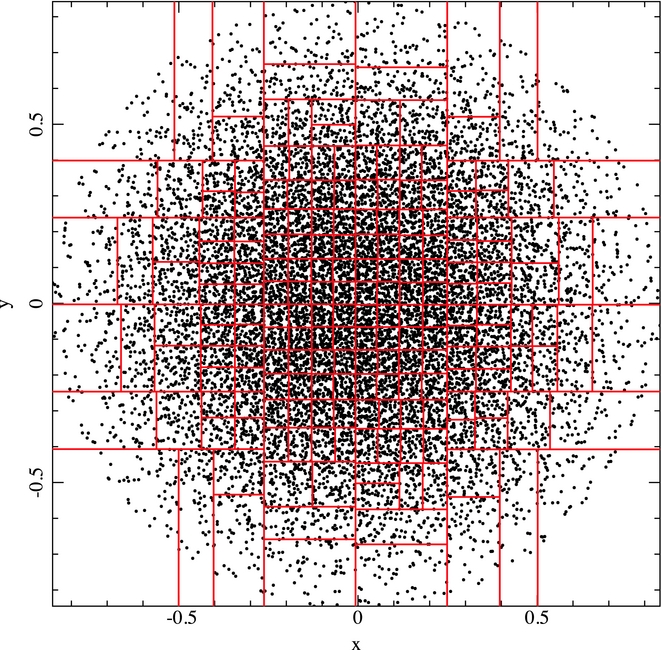
A key optimisation strategy employed in Phantom is to perform the neighbour search for groups of particles. The results of this search (i.e. positions of all trial neighbours) are then cached and used to check for neighbours for individual particles in the group. Our kd-tree algorithm closely follows Gafton & Rosswog (Reference Gafton and Rosswog2011), splitting the particles recursively based on the centre of mass and bisecting the longest axis at each level (Figure 2). The tree build is refined until a cell contains less than N min particles, which is then referred to as a ‘leaf node’. By default, N min = 10. The neighbour search is then performed once for each leaf node. Further details are given in Appendix A.3.1.
Example of the kd-tree build. For illustrative purposes only, we have constructed a 2D version of the tree on the projected particle distribution in the x–y plane of the particle distribution from a polytrope test with 13 115 particles. Each level of the tree recursively splits the particle distribution in half, bisecting the longest axis at the centre of mass until the number of particles in a given cell is <N min. For clarity, we have used N min = 100 in the above example, while N min = 10 by default.
2.2. Hydrodynamics
2.2.1. Compressible hydrodynamics
The equations of compressible hydrodynamics are solved in the form
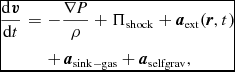 $$\begin{eqnarray}
\frac{{\rm d}{\bm v}}{{\rm d}t} &=& -\frac{\nabla P}{\rho } + \Pi _{\rm shock} + {\bm a}_{\rm ext}({\bm r}, t) \nonumber \\
&& +\, {\bm a}_{\rm sink-gas} + {\bm a}_{\rm selfgrav},
\end{eqnarray}$$
$$\begin{eqnarray}
\frac{{\rm d}{\bm v}}{{\rm d}t} &=& -\frac{\nabla P}{\rho } + \Pi _{\rm shock} + {\bm a}_{\rm ext}({\bm r}, t) \nonumber \\
&& +\, {\bm a}_{\rm sink-gas} + {\bm a}_{\rm selfgrav},
\end{eqnarray}$$
 \begin{align}
\frac{{\rm d}u}{{\rm d}t} = -\frac{P}{\rho } \left(\nabla \cdot {\bm v}\right) + \Lambda _{\rm shock} - \frac{\Lambda _{\rm cool}}{\rho },
\end{align}
\begin{align}
\frac{{\rm d}u}{{\rm d}t} = -\frac{P}{\rho } \left(\nabla \cdot {\bm v}\right) + \Lambda _{\rm shock} - \frac{\Lambda _{\rm cool}}{\rho },
\end{align}
where P is the pressure, u is the specific internal energy,  ${\bm a}_{\rm ext}$, ${\bm a}_{\rm sink-gas}$ and ${\bm a}_{\rm selfgrav}$ refer to (optional) accelerations from ‘external’ or ‘body’ forces (Section 2.4), sink particles (Section 2.8), and self-gravity (Section 2.12), respectively. Πshock and Λshock are dissipation terms required to give the correct entropy increase at a shock front, and Λcool is a cooling term.
2.2.2. Equation of state
The equation set is closed by an equation of state (EOS) relating the pressure to the density and/or internal energy. For an ideal gas, this is given by
 $$\begin{equation}
P = (\gamma - 1)\rho u,
\end{equation}$$
$$\begin{equation}
P = (\gamma - 1)\rho u,
\end{equation}$$
where γ is the adiabatic index and the sound speed c s is given by
 $$\begin{equation}
c_{\rm s} = \sqrt{\frac{\gamma P}{\rho }}.
\end{equation}$$
$$\begin{equation}
c_{\rm s} = \sqrt{\frac{\gamma P}{\rho }}.
\end{equation}$$
The internal energy, u, can be related to the gas temperature, T, using
 $$\begin{equation}
P = \frac{\rho k_{\rm B} T}{\mu m_{\rm H}},
\end{equation}$$
$$\begin{equation}
P = \frac{\rho k_{\rm B} T}{\mu m_{\rm H}},
\end{equation}$$
giving
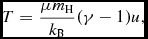 $$\begin{equation}
T = \frac{\mu m_{\rm H}}{k_{\rm B}} (\gamma -1) u,
\end{equation}$$
$$\begin{equation}
T = \frac{\mu m_{\rm H}}{k_{\rm B}} (\gamma -1) u,
\end{equation}$$
where k B is Boltzmann’s constant, μ is the mean molecular weight, and m H is the mass of a hydrogen atom. Thus, to infer the temperature, one needs to specify a composition, but only the internal energy affects the gas dynamics. Equation (25) with γ = 5/3 is the default EOS in Phantom.
In the case where shocks are assumed to radiate away all of the heat generated at the shock front (i.e. Λshock = 0) and there is no cooling (Λcool = 0), (24) becomes simply, using (2)
 $$\begin{equation}
\frac{{\rm d} u}{{\rm d} t} = \frac{P}{\rho ^{2}} \frac{{\rm d}\rho }{{\rm d}t},
\end{equation}$$
$$\begin{equation}
\frac{{\rm d} u}{{\rm d} t} = \frac{P}{\rho ^{2}} \frac{{\rm d}\rho }{{\rm d}t},
\end{equation}$$
which, using (25) can be integrated to give
 $$\begin{equation}
P = K \rho ^{\gamma },
\end{equation}$$
$$\begin{equation}
P = K \rho ^{\gamma },
\end{equation}$$
where K is the polytropic constant. Even more simply, in the case where the temperature is assumed constant, or prescribed as a function of position, the EOS is simply
 $$\begin{equation}
P = c_{\rm s}^{2} \rho .
\end{equation}$$
$$\begin{equation}
P = c_{\rm s}^{2} \rho .
\end{equation}$$
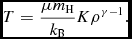
In both of these cases, (30) and (31), the internal energy does not need to be stored. In this case, the temperature is effectively set by the value of K (and the density if γ ≠ 1). Specifically,
 $$\begin{equation}
T = \frac{\mu m_{\rm H}}{k_{\rm B}} K \rho ^{\gamma - 1}.
\end{equation}$$
$$\begin{equation}
T = \frac{\mu m_{\rm H}}{k_{\rm B}} K \rho ^{\gamma - 1}.
\end{equation}$$
2.2.3. Code units
For pure hydrodynamics, physical units are irrelevant to the numerical results since (1)–(2) and (23)–(24) are scale free to all but the Mach number. Hence, setting physical units is only useful when comparing simulations with Nature, when physical heating or cooling rates are applied via (24), or when one wishes to interpret the results in terms of temperature using (28) or (32).
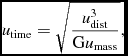
In the case where gravitational forces are applied, either using an external force (Section 2.4) or using self-gravity (Section 2.12), we adopt the standard procedure of transforming units such that G = 1 in code units, i.e.
 $$\begin{equation}
u_{\rm time} = \sqrt{\frac{u_{\rm dist}^{3}}{{\rm G}u_{\rm mass}}},
\end{equation}$$
$$\begin{equation}
u_{\rm time} = \sqrt{\frac{u_{\rm dist}^{3}}{{\rm G}u_{\rm mass}}},
\end{equation}$$
where u time, u dist, and u mass are the units of time, length, and mass, respectively. Additional constraints apply when using relativistic terms (Section 2.4.5) or magnetic fields (Section 2.10.3).
2.2.4. Equation of motion in SPH
We follow the variable smoothing length formulation described by Price (Reference Price2012a), Price & Federrath (Reference Price and Federrath2010), and Lodato & Price (Reference Lodato and Price2010). We discretise (23) using
 $$\begin{eqnarray}
\frac{{\rm d}{\bm v}_{a}}{{\rm d}t} &= & - \sum _{b} m_{b} \left[ \frac{P_{a} + q^{a}_{ab}}{\rho _{a}^{2}\Omega _{a}}\nabla _a W_{ab}(h_{a}) + \frac{P_{b}+q^{b}_{ab}}{\rho _{b}^{2}\Omega _{b}}\nabla _a W_{ab}(h_{b}) \right] \nonumber \\
&& +\, {\bm a}_{\rm ext} ({\bm r}_{a}, t) + {\bm a}^{a}_{\rm sink-gas} + {\bm a}^{a}_{\rm selfgrav},
\end{eqnarray}$$
$$\begin{eqnarray}
\frac{{\rm d}{\bm v}_{a}}{{\rm d}t} &= & - \sum _{b} m_{b} \left[ \frac{P_{a} + q^{a}_{ab}}{\rho _{a}^{2}\Omega _{a}}\nabla _a W_{ab}(h_{a}) + \frac{P_{b}+q^{b}_{ab}}{\rho _{b}^{2}\Omega _{b}}\nabla _a W_{ab}(h_{b}) \right] \nonumber \\
&& +\, {\bm a}_{\rm ext} ({\bm r}_{a}, t) + {\bm a}^{a}_{\rm sink-gas} + {\bm a}^{a}_{\rm selfgrav},
\end{eqnarray}$$
where the qaab and qbab terms represent the artificial viscosity (discussed in Section 2.2.7).
2.2.5. Internal energy equation
The internal energy equation (24) is discretised using the time derivative of the density sum (c.f. 29), which from (4) gives
 $$\begin{equation}
\frac{{\rm d} u_{a}}{{\rm d} t} = \frac{P_{a}}{\rho _{a}^{2}\Omega _{a}} \sum _{b} m_{b} {\bm v}_{ab} \cdot \nabla _{a} W_{ab} (h_{a}) + \Lambda _{\rm shock} - \frac{\Lambda _{\rm cool}}{\rho },
\end{equation}$$
$$\begin{equation}
\frac{{\rm d} u_{a}}{{\rm d} t} = \frac{P_{a}}{\rho _{a}^{2}\Omega _{a}} \sum _{b} m_{b} {\bm v}_{ab} \cdot \nabla _{a} W_{ab} (h_{a}) + \Lambda _{\rm shock} - \frac{\Lambda _{\rm cool}}{\rho },
\end{equation}$$
where  ${\bm v}_{ab} \equiv {\bm v}_a - {\bm v}_b$. In the variational formulation of SPH (e.g. Price Reference Price2012a), this expression is used as a constraint to derive (34), which guarantees both the conservation of energy and entropy (the latter in the absence of dissipation terms). The shock capturing terms in the internal energy equation are discussed below.
By default, we assume an adiabatic gas, meaning that PdV work and shock heating terms contribute to the thermal energy of the gas, no energy is radiated to the environment, and total energy is conserved. To approximate a radiative gas, one may set one or both of these terms to zero. Neglecting the shock heating term, Λshock, gives an approximation equivalent to a polytropic EOS (30), as described in Section 2.2.2. Setting both shock and work contributions to zero implies that du/dt = 0, meaning that each particle will simply retain its initial temperature.
2.2.6. Conservation of energy in SPH
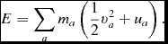
Does evolving the internal energy equation imply that total energy is not conserved? Wrong! Total energy in SPH, for the case of hydrodynamics, is given by
 $$\begin{equation}
E = \sum _a m_a \left(\frac{1}{2} v_a^2 + u_a\right).
\end{equation}$$
$$\begin{equation}
E = \sum _a m_a \left(\frac{1}{2} v_a^2 + u_a\right).
\end{equation}$$
Taking the (Lagrangian) time derivative, we find that conservation of energy corresponds to
 $$\begin{equation}
\frac{{\rm d}E}{{\rm d}t} = \sum _{a} m_{a} \left( {\bm v}_{a} \cdot \frac{{\rm d} {\bm v}_{a}}{{\rm d} t} + \frac{{\rm d} u_{a}}{{\rm d} t} \right) = 0.
\end{equation}$$
$$\begin{equation}
\frac{{\rm d}E}{{\rm d}t} = \sum _{a} m_{a} \left( {\bm v}_{a} \cdot \frac{{\rm d} {\bm v}_{a}}{{\rm d} t} + \frac{{\rm d} u_{a}}{{\rm d} t} \right) = 0.
\end{equation}$$
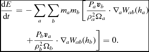
Inserting our expressions (34) and (35), and neglecting for the moment dissipative terms and external forces, we find
 $$\begin{eqnarray}
\frac{{\rm d}E}{{\rm d}t} &=& -\sum _{a} \sum _{b} m_{a} m_{b} \left[ \frac{P_{a}\bm {v}_b}{\rho _{a}^{2}\Omega _{a}}\cdot \nabla _a W_{ab}(h_{a}) \right. \nonumber \\
&& \left. + \frac{P_{b}\bm {v}_a}{\rho _{b}^{2}\Omega _{b}}\cdot \nabla _a W_{ab}(h_{b}) \right] = 0.
\end{eqnarray}$$
$$\begin{eqnarray}
\frac{{\rm d}E}{{\rm d}t} &=& -\sum _{a} \sum _{b} m_{a} m_{b} \left[ \frac{P_{a}\bm {v}_b}{\rho _{a}^{2}\Omega _{a}}\cdot \nabla _a W_{ab}(h_{a}) \right. \nonumber \\
&& \left. + \frac{P_{b}\bm {v}_a}{\rho _{b}^{2}\Omega _{b}}\cdot \nabla _a W_{ab}(h_{b}) \right] = 0.
\end{eqnarray}$$
The double summation on the right-hand side equals zero because the kernel gradient, and hence the overall sum, is antisymmetric. That is, ∇aW ab = −∇bW ba. This means one can relabel the summation indices arbitrarily in one half of the sum, and add it to one half of the original sum to give zero. One may straightforwardly verify that this remains true when one includes the dissipative terms (see below).
This means that even though we employ the internal energy equation, total energy remains conserved to machine precision in the spatial discretisation. That is, energy is conserved irrespective of the number of particles, the number of neighbours or the choice of smoothing kernel. The only non-conservation of energy arises from the ordinary differential equation solver one employs to solve the left-hand side of the equations. We thus employ a symplectic time integration scheme in order to preserve the conservation properties as accurately as possible (Section 2.3.1).
2.2.7. Shock capturing: momentum equation
The shock capturing dissipation terms are implemented following Monaghan (Reference Monaghan1997), derived by analogy with Riemann solvers from the special relativistic dissipation terms proposed by Chow & Monaghan (Reference Chow and Monaghan1997). These were extended by Price & Monaghan (Reference Price and Monaghan2004b, Reference Price and Monaghan2005) to MHD and recently to dust–gas mixtures by Laibe & Price (Reference Laibe and Price2014b). In a recent paper, Puri & Ramachandran (Reference Puri and Ramachandran2014) found this approach, along with the Morris & Monaghan (Reference Morris and Monaghan1997) switch (which they referred to as the ‘Monaghan–Price–Morris’ formulation) to be the most accurate and robust method for shock capturing in SPH when compared to several other approaches, including Godunov SPH (e.g. Inutsuka Reference Inutsuka2002; Cha & Whitworth Reference Cha and Whitworth2003).
The formulation in Phantom differs from that given in Price (Reference Price2012a) only by the way that the density and signal speed in the q terms are averaged, as described in Price & Federrath (Reference Price and Federrath2010) and Lodato & Price (Reference Lodato and Price2010). That is, we use
 $$\begin{equation}
\Pi _{\rm shock}^{a} \equiv -\sum _{b} m_{b} \left[ \frac{q^{a}_{ab}}{\rho _{a}^{2}\Omega _{a}}\nabla _a W_{ab}(h_{a}) + \frac{q^{b}_{ab}}{\rho _{b}^{2}\Omega _{b}}\nabla _a W_{ab}(h_{b}) \right],
\end{equation}$$
$$\begin{equation}
\Pi _{\rm shock}^{a} \equiv -\sum _{b} m_{b} \left[ \frac{q^{a}_{ab}}{\rho _{a}^{2}\Omega _{a}}\nabla _a W_{ab}(h_{a}) + \frac{q^{b}_{ab}}{\rho _{b}^{2}\Omega _{b}}\nabla _a W_{ab}(h_{b}) \right],
\end{equation}$$
where
 $$\begin{equation}
q^{a}_{ab} = \left\lbrace \arraycolsep5pt\begin{array}{@{}ll@{}}-\displaystyle\frac{1}{2} \rho _{a} v_{{\rm sig}, a} {\bm v}_{ab} \cdot \hat{\bm r}_{ab}, & {\bm v}_{ab} \cdot \hat{\bm r}_{ab} < 0 \\[6pt]
0 & \text{otherwise,} \end{array}\right.
\end{equation}$$
$$\begin{equation}
q^{a}_{ab} = \left\lbrace \arraycolsep5pt\begin{array}{@{}ll@{}}-\displaystyle\frac{1}{2} \rho _{a} v_{{\rm sig}, a} {\bm v}_{ab} \cdot \hat{\bm r}_{ab}, & {\bm v}_{ab} \cdot \hat{\bm r}_{ab} < 0 \\[6pt]
0 & \text{otherwise,} \end{array}\right.
\end{equation}$$
where  ${\bm v}_{ab} \equiv {\bm v}_{a} - {\bm v}_{b}$, $\hat{\bm r}_{ab} \equiv ({\bm r}_{a} - {\bm r}_{b})/\vert {\bm r}_{a} - {\bm r}_{b} \vert$ is the unit vector along the line of sight between the particles, and v sig is the maximum signal speed, which depends on the physics implemented. For hydrodynamics, this is given by
 $$\begin{equation}
v_{{\rm sig},a} = \alpha ^{\rm AV}_{a} c_{{\rm s},a} + \beta ^{\rm AV} \vert {\bm v}_{ab} \cdot \hat{\bm r}_{ab} \vert ,
\end{equation}$$
$$\begin{equation}
v_{{\rm sig},a} = \alpha ^{\rm AV}_{a} c_{{\rm s},a} + \beta ^{\rm AV} \vert {\bm v}_{ab} \cdot \hat{\bm r}_{ab} \vert ,
\end{equation}$$
where in general αAVa ∈ [0, 1] is controlled by a switch (see Section 2.2.9), while βAV = 2 by default.
Importantly, α does not multiply the βAV term. The βAV term provides a second-order Von Neumann & Richtmyer-like term that prevents particle interpenetration (e.g. Lattanzio et al. Reference Lattanzio, Monaghan, Pongracic and Schwarz1986; Monaghan Reference Monaghan1989), and thus βAV ⩾ 2 is needed wherever particle penetration may occur. This is important in accretion disc simulations where use of a low α may be acceptable in the absence of strong shocks, but a low β will lead to particle penetration of the disc midplane, which is the cause of a number of convergence issues (Meru & Bate Reference Meru and Bate2011, Reference Meru and Bate2012). Price & Federrath (Reference Price and Federrath2010) found that βAV = 4 was necessary at high Mach number (M ≳ 5) to maintain a sharp shock structure, which despite nominally increasing the viscosity was found to give less dissipation overall because particle penetration no longer occurred at shock fronts.
2.2.8. Shock capturing: internal energy equation
The key insight from Chow & Monaghan (Reference Chow and Monaghan1997) was that shock capturing not only involves a viscosity term but involves dissipating the jump in each component of the energy, implying a conductivity term in hydrodynamics and resistive dissipation in MHD (see Section 2.10.5). The resulting contribution to the internal energy equation is given by (e.g. Price Reference Price2012a)
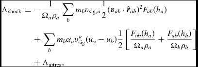 $$\begin{eqnarray}
\Lambda _{\rm shock} & \equiv& - \frac{1}{\Omega _{a}\rho _a} \sum _{b} m_{b} v_{{\rm sig}, a} \frac{1}{2} ({\bm v}_{ab} \cdot \hat{\bm r}_{ab})^{2} F_{ab}(h_{a}) \nonumber \\
&& +\, \sum _{b} m_{b} \alpha _{u} v^{u}_{\rm sig} (u_{a} - u_{b}) \frac{1}{2} \left[ \frac{F_{ab} (h_{a})}{\Omega _{a} \rho _{a}} + \frac{F_{ab} (h_{b})}{\Omega _{b} \rho _{b}} \right] \nonumber \\
&& +\, \Lambda _{\rm artres},
\end{eqnarray}$$
$$\begin{eqnarray}
\Lambda _{\rm shock} & \equiv& - \frac{1}{\Omega _{a}\rho _a} \sum _{b} m_{b} v_{{\rm sig}, a} \frac{1}{2} ({\bm v}_{ab} \cdot \hat{\bm r}_{ab})^{2} F_{ab}(h_{a}) \nonumber \\
&& +\, \sum _{b} m_{b} \alpha _{u} v^{u}_{\rm sig} (u_{a} - u_{b}) \frac{1}{2} \left[ \frac{F_{ab} (h_{a})}{\Omega _{a} \rho _{a}} + \frac{F_{ab} (h_{b})}{\Omega _{b} \rho _{b}} \right] \nonumber \\
&& +\, \Lambda _{\rm artres},
\end{eqnarray}$$
where the first term provides the viscous shock heating, the second term provides an artificial thermal conductivity, F ab is defined as in (15), and Λartres is the heating due to artificial resistivity [Equation (182)]. The signal speed we use for conductivity term differs from the one used for viscosity, as discussed by Price (Reference Price2008, Reference Price2012a). In Phantom, we use
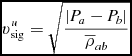 $$\begin{equation}
v^{u}_{\rm sig} = \sqrt{\frac{\vert P_{a} - P_{b} \vert }{\overline{\rho }_{ab}}}
\end{equation}$$
$$\begin{equation}
v^{u}_{\rm sig} = \sqrt{\frac{\vert P_{a} - P_{b} \vert }{\overline{\rho }_{ab}}}
\end{equation}$$
for simulations that do not involve self-gravity or external body forces (Price Reference Price2008), and
 $$\begin{equation}
v^{u}_{\rm sig} = \vert {\bm v}_{ab} \cdot \hat{\bm r}_{ab} \vert
\end{equation}$$
$$\begin{equation}
v^{u}_{\rm sig} = \vert {\bm v}_{ab} \cdot \hat{\bm r}_{ab} \vert
\end{equation}$$
for simulations that do (Wadsley, Veeravalli, & Couchman Reference Wadsley, Veeravalli and Couchman2008). The importance of the conductivity term for treating contact discontinuities was highlighted by Price (Reference Price2008), explaining the poor results found by Agertz et al. (Reference Agertz2007) in SPH simulations of Kelvin–Helmholtz instabilities run across contact discontinuities (discussed further in Section 5.1.4). With (44), we have found there is no need for further switches to reduce conductivity (e.g. Price Reference Price2004; Price & Monaghan Reference Price and Monaghan2005; Valdarnini Reference Valdarnini2016), since the effective thermal conductivity κ is second order in the smoothing length (∝h 2). Phantom therefore uses αu = 1 by default in (42) and we have not yet found a situation where this leads to excess smoothing.
It may be readily shown that the total energy remains conserved in the presence of dissipation by combining (42) with the corresponding dissipative terms in (34). The contribution to the entropy from both viscosity and conductivity is also positive definite (see the appendix in Price & Monaghan Reference Price and Monaghan2004b for the mathematical proof in the case of conductivity).
2.2.9. Shock detection
The standard approach to reducing dissipation in SPH away from shocks for the last 15 yr has been the switch proposed by Morris & Monaghan (Reference Morris and Monaghan1997), where the dimensionless viscosity parameter α is evolved for each particle a according to
 $$\begin{equation}
\frac{{\rm d}\alpha _{a}}{{\rm d}t} = \max (-\nabla \cdot {\bm v}_{a}, 0) - \frac{(\alpha _{a} - \alpha _{\rm min})}{\tau _{a}},
\end{equation}$$
$$\begin{equation}
\frac{{\rm d}\alpha _{a}}{{\rm d}t} = \max (-\nabla \cdot {\bm v}_{a}, 0) - \frac{(\alpha _{a} - \alpha _{\rm min})}{\tau _{a}},
\end{equation}$$
where τ ≡ h/(σdecayv sig) and σdecay = 0.1 by default. We set v sig in the decay time equal to the sound speed to avoid the need to store dα/dt, since  $\nabla \cdot {\bm v}$ is already stored in order to compute (4). This is the switch used for numerous turbulence applications with Phantom (e.g. Price & Federrath Reference Price and Federrath2010; Price et al. Reference Price, Federrath and Brunt2011; Tricco et al. Reference Tricco, Price and Federrath2016b) where it is important to minimise numerical dissipation in order to maximise the Reynolds number (e.g. Valdarnini Reference Valdarnini2011; Price Reference Price2012b).
More recently, Cullen & Dehnen (Reference Cullen and Dehnen2010) proposed a more advanced switch using the time derivative of the velocity divergence. A modified version based on the gradient of the velocity divergence was also proposed by Read & Hayfield (Reference Read and Hayfield2012). We implement a variation on the Cullen & Dehnen (Reference Cullen and Dehnen2010) switch, using a shock indicator of the form
 $$\begin{equation}
A_{a} = \xi _{a} \max \left[-\frac{{\rm d}}{{\rm d}t}(\nabla \cdot {\bm v}_{a}), 0 \right] ,
\end{equation}$$
$$\begin{equation}
A_{a} = \xi _{a} \max \left[-\frac{{\rm d}}{{\rm d}t}(\nabla \cdot {\bm v}_{a}), 0 \right] ,
\end{equation}$$
where
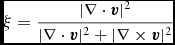 $$\begin{equation}
\xi = \frac{\vert \nabla \cdot {\bm v} \vert ^{2}}{\vert \nabla \cdot {\bm v} \vert ^{2} + \vert \nabla \times {\bm v} \vert ^{2}}
\end{equation}$$
$$\begin{equation}
\xi = \frac{\vert \nabla \cdot {\bm v} \vert ^{2}}{\vert \nabla \cdot {\bm v} \vert ^{2} + \vert \nabla \times {\bm v} \vert ^{2}}
\end{equation}$$
is a modification of the Balsara (Reference Balsara1995) viscosity limiter for shear flows. We use this to set α according to
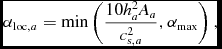 $$\begin{equation}
\alpha _{{\rm loc}, a} =\min \left( \frac{10 h_{a}^{2} A_{a}}{c_{{\rm s}, a}^{2}}, \alpha _{\rm max} \right),
\end{equation}$$
$$\begin{equation}
\alpha _{{\rm loc}, a} =\min \left( \frac{10 h_{a}^{2} A_{a}}{c_{{\rm s}, a}^{2}}, \alpha _{\rm max} \right),
\end{equation}$$
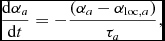
where c s is the sound speed and αmax = 1. We use c s in the expression for αloc also for MHD (Section 2.10) since we found using the magnetosonic speed led to a poor treatment of MHD shocks. If αloc, a > αa, we set αa = αloc, a, otherwise we evolve αa according to
 $$\begin{equation}
\frac{{\rm d}\alpha _{a}}{{\rm d}t} = - \frac{(\alpha _{a} - \alpha _{{\rm loc}, a})}{\tau _{a}},
\end{equation}$$
$$\begin{equation}
\frac{{\rm d}\alpha _{a}}{{\rm d}t} = - \frac{(\alpha _{a} - \alpha _{{\rm loc}, a})}{\tau _{a}},
\end{equation}$$
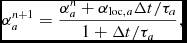
where τ is defined as in the Morris & Monaghan (Reference Morris and Monaghan1997) version, above. We evolve α in the predictor part of the integrator only, i.e. with a first-order time integration, to avoid complications in the corrector step. However, we perform the predictor step implicitly using a backward Euler method, i.e.
 $$\begin{equation}
\alpha ^{n+1}_{a} = \frac{\alpha _{a}^{n} + \alpha _{{\rm loc}, a} \Delta t / \tau _{a}}{1 + \Delta t / \tau _{a}},
\end{equation}$$
$$\begin{equation}
\alpha ^{n+1}_{a} = \frac{\alpha _{a}^{n} + \alpha _{{\rm loc}, a} \Delta t / \tau _{a}}{1 + \Delta t / \tau _{a}},
\end{equation}$$
which ensures that the decay is stable regardless of the timestep (we do this for the Morris & Monaghan method also).
We use the method outlined in Appendix B3 of Cullen & Dehnen (Reference Cullen and Dehnen2010) to compute 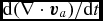 ${\rm d}(\nabla \cdot {\bm v}_{a})/{{\rm d}t}$. That is, we first compute the gradient tensors of the velocity, ${\bm v}$, and acceleration, ${\bm a}$ (used from the previous timestep), during the density loop using an SPH derivative operator that is exact to linear order, that is, with the matrix correction outlined in Price (Reference Price2004, Reference Price2012a), namely
 $$\begin{equation}
R^{ij}_{a} \frac{\partial v^{k}_{a}}{\partial x^{j}_{a}} = \sum _{b} m_{b} \left(v^{k}_{b} - v^{k}_{a}\right) \frac{\partial W_{ab}(h_{a})}{\partial x^{i}} ,
\end{equation}$$
$$\begin{equation}
R^{ij}_{a} \frac{\partial v^{k}_{a}}{\partial x^{j}_{a}} = \sum _{b} m_{b} \left(v^{k}_{b} - v^{k}_{a}\right) \frac{\partial W_{ab}(h_{a})}{\partial x^{i}} ,
\end{equation}$$
where
 $$\begin{equation}
R^{ij}_{a} = \sum _{b} m_{b} \left(x^{i}_{b} - x^{i}_{a}\right) \frac{\partial W_{ab}(h_{a})}{\partial x^{j}} \approx \delta ^{ij},
\end{equation}$$
$$\begin{equation}
R^{ij}_{a} = \sum _{b} m_{b} \left(x^{i}_{b} - x^{i}_{a}\right) \frac{\partial W_{ab}(h_{a})}{\partial x^{j}} \approx \delta ^{ij},
\end{equation}$$
and repeated tensor indices imply summation. Finally, we construct the time derivative of the velocity divergence according to
 $$\begin{equation}
\frac{{\rm d}}{{\rm d}t}\left(\frac{\partial v_{a}^{i}}{\partial x_{a}^{i}}\right) = \frac{\partial a_{a}^{i}}{\partial x_{a}^{i}} - \frac{\partial v_{a}^{i}}{\partial x_{a}^{j}} \frac{\partial v_{a}^{j}}{\partial x_{a}^{i}},
\end{equation}$$
$$\begin{equation}
\frac{{\rm d}}{{\rm d}t}\left(\frac{\partial v_{a}^{i}}{\partial x_{a}^{i}}\right) = \frac{\partial a_{a}^{i}}{\partial x_{a}^{i}} - \frac{\partial v_{a}^{i}}{\partial x_{a}^{j}} \frac{\partial v_{a}^{j}}{\partial x_{a}^{i}},
\end{equation}$$
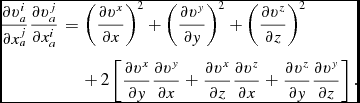
where, as previously, repeated i and j indices imply summation. In Cartesian coordinates, the last term in (53) can be written out explicitly using
 $$\begin{eqnarray}
\frac{\partial v_{a}^{i}}{\partial x_{a}^{j}} \frac{\partial v_{a}^{j}}{\partial x_{a}^{i}} & =& \left(\frac{\partial v^{x}}{\partial x} \right)^{2} + \left(\frac{\partial v^{y}}{\partial y} \right)^{2} + \left(\frac{\partial v^{z}}{\partial z} \right)^{2} \nonumber \\
& &+\, 2 \left[\frac{\partial v^{x}}{\partial y} \frac{\partial v^{y}}{\partial x} + \frac{\partial v^{x}}{\partial z} \frac{\partial v^{z}}{\partial x} + \frac{\partial v^{z}}{\partial y} \frac{\partial v^{y}}{\partial z}\right].
\end{eqnarray}$$
$$\begin{eqnarray}
\frac{\partial v_{a}^{i}}{\partial x_{a}^{j}} \frac{\partial v_{a}^{j}}{\partial x_{a}^{i}} & =& \left(\frac{\partial v^{x}}{\partial x} \right)^{2} + \left(\frac{\partial v^{y}}{\partial y} \right)^{2} + \left(\frac{\partial v^{z}}{\partial z} \right)^{2} \nonumber \\
& &+\, 2 \left[\frac{\partial v^{x}}{\partial y} \frac{\partial v^{y}}{\partial x} + \frac{\partial v^{x}}{\partial z} \frac{\partial v^{z}}{\partial x} + \frac{\partial v^{z}}{\partial y} \frac{\partial v^{y}}{\partial z}\right].
\end{eqnarray}$$
2.2.10. Cooling
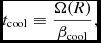
The cooling term Λcool can be set either from detailed chemical calculations (Section 2.14.1) or, for discs, by the simple ‘β-cooling’ prescription of Gammie (Reference Gammie2001), namely
 $$\begin{equation}
\Lambda _{\rm cool} = \frac{\rho u}{t_{\rm cool}},
\end{equation}$$
$$\begin{equation}
\Lambda _{\rm cool} = \frac{\rho u}{t_{\rm cool}},
\end{equation}$$
where
 $$\begin{equation}
t_{\rm cool} \equiv \frac{\Omega (R)}{\beta _{\rm cool}},
\end{equation}$$
$$\begin{equation}
t_{\rm cool} \equiv \frac{\Omega (R)}{\beta _{\rm cool}},
\end{equation}$$
with βcool an input parameter to the code specifying the cooling timescale in terms of the local orbital time. We compute Ω in (56) using Ω ≡ 1/(x 2 + y 2 + z 2)3/2, i.e. assuming Keplerian rotation around a central object with mass equal to unity, with G = 1 in code units.
2.2.11. Conservation of linear and angular momentum
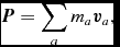
The total linear momentum is given by
 $$\begin{equation}
\bm {P} = \sum _{a} m_{a} {\bm v}_{a},
\end{equation}$$
$$\begin{equation}
\bm {P} = \sum _{a} m_{a} {\bm v}_{a},
\end{equation}$$
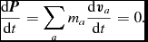
such that conservation of momentum corresponds to
 $$\begin{equation}
\frac{{\rm d}\bm {P}}{{\rm d}t} = \sum _{a} m_{a} \frac{{\rm d}{\bm v}_{a}}{{\rm d}t} = 0.
\end{equation}$$
$$\begin{equation}
\frac{{\rm d}\bm {P}}{{\rm d}t} = \sum _{a} m_{a} \frac{{\rm d}{\bm v}_{a}}{{\rm d}t} = 0.
\end{equation}$$
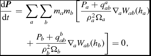
Inserting our discrete equation (34), we find
 $$\begin{eqnarray}
\frac{{\rm d}\bm {P}}{{\rm d}t} &=& \sum _{a} \sum _{b} m_a m_{b} \left[ \frac{P_{a} + q^{a}_{ab}}{\rho _{a}^{2}\Omega _{a}}\nabla _a W_{ab}(h_{a}) \right. \nonumber \\
&& \left. +\, \frac{P_{b}+q^{b}_{ab}}{\rho _{b}^{2}\Omega _{b}}\nabla _a W_{ab}(h_{b}) \right] = 0,
\end{eqnarray}$$
$$\begin{eqnarray}
\frac{{\rm d}\bm {P}}{{\rm d}t} &=& \sum _{a} \sum _{b} m_a m_{b} \left[ \frac{P_{a} + q^{a}_{ab}}{\rho _{a}^{2}\Omega _{a}}\nabla _a W_{ab}(h_{a}) \right. \nonumber \\
&& \left. +\, \frac{P_{b}+q^{b}_{ab}}{\rho _{b}^{2}\Omega _{b}}\nabla _a W_{ab}(h_{b}) \right] = 0,
\end{eqnarray}$$
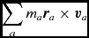
where, as for the total energy (Section 2.2.6), the double summation is zero because of the antisymmetry of the kernel gradient. The same argument applies to the conservation of angular momentum,
 $$\begin{equation}
\sum _{a} m_{a} {\bm r}_{a} \times {\bm v}_{a}
\end{equation}$$
$$\begin{equation}
\sum _{a} m_{a} {\bm r}_{a} \times {\bm v}_{a}
\end{equation}$$
(see e.g. Price Reference Price2012a for a detailed proof). As with total energy, this means linear and angular momentum are exactly conserved by our SPH scheme to the accuracy with which they are conserved by the timestepping scheme.
In Phantom, linear and angular momentum are both conserved to round-off error (typically ~10−16 in double precision) with global timestepping, but exact conservation is violated when using individual particle timesteps or when using the kd-tree to compute gravitational forces. The magnitude of these quantities, as well as the total energy and the individual components of energy (kinetic, internal, potential, and magnetic), should thus be monitored by the user at runtime. Typically with individual timesteps, one should expect energy conservation to ΔE/E ~ 10−3 and linear and angular momentum conservation to ~10−6 with default code settings. The code execution is aborted if conservation errors exceed 10%.
2.3. Time integration
2.3.1. Timestepping algorithm
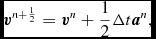
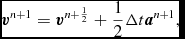
We integrate the equations of motion using a generalisation of the Leapfrog integrator which is reversible in the case of both velocity dependent forces and derivatives which depend on the velocity field. The basic integrator is the Leapfrog method in ‘Kick–Drift–Kick’ or ‘Velocity Verlet’ form (Verlet Reference Verlet1967), where the positions and velocities of particles are updated from time t n to t n + 1 according to
 $$\begin{eqnarray}
{\bm v}^{n+\frac{1}{2}} = {\bm v}^{n} + \frac{1}{2} \Delta t {\bm a}^{n},
\end{eqnarray}$$
$$\begin{eqnarray}
{\bm v}^{n+\frac{1}{2}} = {\bm v}^{n} + \frac{1}{2} \Delta t {\bm a}^{n},
\end{eqnarray}$$
 $$\begin{eqnarray}
{\bm r}^{n+1} = {\bm r}^{n} + \Delta t {\bm v}^{n+\frac{1}{2}},
\end{eqnarray}$$
$$\begin{eqnarray}
{\bm r}^{n+1} = {\bm r}^{n} + \Delta t {\bm v}^{n+\frac{1}{2}},
\end{eqnarray}$$
 $$\begin{eqnarray}
{\bm a}^{n + 1} = {\bm a}({\bm r}^{n+1}),
\end{eqnarray}$$
$$\begin{eqnarray}
{\bm a}^{n + 1} = {\bm a}({\bm r}^{n+1}),
\end{eqnarray}$$
 $$\begin{eqnarray}
{\bm v}^{n + 1} = {\bm v}^{n+\frac{1}{2}} + \frac{1}{2} \Delta t {\bm a}^{n+1},
\end{eqnarray}$$
$$\begin{eqnarray}
{\bm v}^{n + 1} = {\bm v}^{n+\frac{1}{2}} + \frac{1}{2} \Delta t {\bm a}^{n+1},
\end{eqnarray}$$
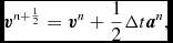
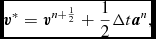
where Δt ≡ t n + 1 − t n. This is identical to the formulation of Leapfrog used in other astrophysical SPH codes (e.g. Springel Reference Springel2005; Wadsley et al. Reference Wadsley, Stadel and Quinn2004). The Verlet scheme, being both reversible and symplectic (e.g. Hairer, Lubich, & Wanner Reference Hairer, Lubich and Wanner2003), preserves the Hamiltonian nature of the SPH algorithm (e.g. Gingold & Monaghan Reference Gingold and Monaghan1982b; Monaghan & Price Reference Monaghan and Price2001). In particular, both linear and angular momentum are exactly conserved, there is no long-term energy drift, and phase space volume is conserved (e.g. for orbital dynamics). In SPH, this is complicated by velocity-dependent terms in the acceleration from the shock-capturing dissipation terms. In this case, the corrector step, (64), becomes implicit. The approach we take is to notice that these terms are not usually dominant over the position-dependent terms. Hence, we use a first-order prediction of the velocity, as follows:
 $$\begin{eqnarray}
{\bm v}^{n+\frac{1}{2}} = {\bm v}^{n} + \frac{1}{2} \Delta t {\bm a}^{n},
\end{eqnarray}$$
$$\begin{eqnarray}
{\bm v}^{n+\frac{1}{2}} = {\bm v}^{n} + \frac{1}{2} \Delta t {\bm a}^{n},
\end{eqnarray}$$
 $$\begin{eqnarray}
{\bm r}^{n+1} = {\bm r}^{n} + \Delta t {\bm v}^{n+\frac{1}{2}},
\end{eqnarray}$$
$$\begin{eqnarray}
{\bm r}^{n+1} = {\bm r}^{n} + \Delta t {\bm v}^{n+\frac{1}{2}},
\end{eqnarray}$$
 $$\begin{eqnarray}
{\bm v}^{*} = {\bm v}^{n+\frac{1}{2}} + \frac{1}{2} \Delta t {\bm a}^{n},
\end{eqnarray}$$
$$\begin{eqnarray}
{\bm v}^{*} = {\bm v}^{n+\frac{1}{2}} + \frac{1}{2} \Delta t {\bm a}^{n},
\end{eqnarray}$$
 $$\begin{eqnarray}
{\bm a}^{n + 1} = {\bm a}({\bm r}^{n+1}, {\bm v}^{*}),
\end{eqnarray}$$
$$\begin{eqnarray}
{\bm a}^{n + 1} = {\bm a}({\bm r}^{n+1}, {\bm v}^{*}),
\end{eqnarray}$$
 $$\begin{eqnarray}
{\bm v}^{n + 1} = {\bm v}^{*} + \frac{1}{2} \Delta t \left[ {\bm a}^{n+1} - {\bm a}^{n} \right].
\end{eqnarray}$$
$$\begin{eqnarray}
{\bm v}^{n + 1} = {\bm v}^{*} + \frac{1}{2} \Delta t \left[ {\bm a}^{n+1} - {\bm a}^{n} \right].
\end{eqnarray}$$
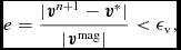
At the end of the step, we then check if the error in the first-order prediction is less than some tolerance ε according to
 $$\begin{equation}
e = \frac{ \vert {\bm v}^{n+1} - {\bm v}^{*} \vert }{ \vert {\bm v}^{\rm mag} \vert } < \epsilon _{\rm v},
\end{equation}$$
$$\begin{equation}
e = \frac{ \vert {\bm v}^{n+1} - {\bm v}^{*} \vert }{ \vert {\bm v}^{\rm mag} \vert } < \epsilon _{\rm v},
\end{equation}$$
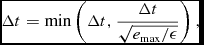
where  ${\bm v}^{\rm mag}$ is the mean velocity on all SPH particles (we set the error to zero if $\vert {\bm v}^{\rm mag}\vert = 0$) and by default εv = 10−2. If this criterion is violated, then we recompute the accelerations by replacing ${\bm v}^{*}$ with ${\bm v}^{n+1}$ and iterating (68) and (69) until the criterion in (70) is satisfied. In practice, this happens rarely, but occurs for example in the first few steps of the Sedov problem where the initial conditions are discontinuous (Section 5.1.3). As each iteration is as expensive as halving the timestep, we also constrain the subsequent timestep such that iterations should not occur, i.e.
 $$\begin{equation}
\Delta t = \min \left( \Delta t, \frac{\Delta t}{\sqrt{e_{\rm max} / \epsilon }} \right),
\end{equation}$$
$$\begin{equation}
\Delta t = \min \left( \Delta t, \frac{\Delta t}{\sqrt{e_{\rm max} / \epsilon }} \right),
\end{equation}$$
where e max = max(e) over all particles. A caveat to the above is that velocity iterations are not currently implemented when using individual particle timesteps.
Additional variables such as the internal energy, u, and the magnetic field,  ${\bm B}$, are timestepped with a predictor and trapezoidal corrector step in the same manner as the velocity, following (65), (67) and (69).
Velocity-dependent external forces are treated separately, as described in Section 2.4.
2.3.2. Timestep constraints
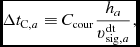
The timestep itself is determined at the end of each step, and is constrained to be less than the maximum stable timestep. For a given particle, a, this is given by (e.g. Lattanzio et al. Reference Lattanzio, Monaghan, Pongracic and Schwarz1986; Monaghan Reference Monaghan1997)
 $$\begin{equation}
\Delta t_{{\rm C},a} \equiv C_{\rm cour} \frac{h_a}{v^{\rm dt}_{{\rm sig},a}},
\end{equation}$$
$$\begin{equation}
\Delta t_{{\rm C},a} \equiv C_{\rm cour} \frac{h_a}{v^{\rm dt}_{{\rm sig},a}},
\end{equation}$$
where C cour = 0.3 by default (Lattanzio et al. Reference Lattanzio, Monaghan, Pongracic and Schwarz1986) and v dtsig is taken as the maximum of (41) over the particle’s neighbours assuming αAV = max(αAV, 1). The criterion above differs from the usual Courant–Friedrichs–Lewy condition used in Eulerian codes (Courant, Friedrichs, & Lewy Reference Courant, Friedrichs and Lewy1928) because it depends only on the difference in velocity between neighbouring particles, not the absolute value.
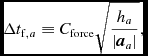
An additional constraint is applied from the accelerations (the ‘force condition’), where
 $$\begin{equation}
\Delta t_{{\rm f}, a} \equiv C_{\rm force} \sqrt{\frac{h_{a}}{\vert {\bm a}_{a} \vert }},
\end{equation}$$
$$\begin{equation}
\Delta t_{{\rm f}, a} \equiv C_{\rm force} \sqrt{\frac{h_{a}}{\vert {\bm a}_{a} \vert }},
\end{equation}$$
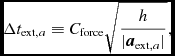
where C force = 0.25 by default. A separate timestep constraint is applied for external forces
 $$\begin{equation}
\Delta t_{{\rm ext},a} \equiv C_{\rm force} \sqrt{\frac{h}{\vert {\bm a}_{{\rm ext},a} \vert }},
\end{equation}$$
$$\begin{equation}
\Delta t_{{\rm ext},a} \equiv C_{\rm force} \sqrt{\frac{h}{\vert {\bm a}_{{\rm ext},a} \vert }},
\end{equation}$$
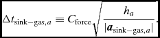
and for accelerations to SPH particles to/from sink particles (Section 2.8)
 $$\begin{equation}
\Delta t_{{\rm sink-gas},a} \equiv C_{\rm force} \sqrt{\frac{h_{a}}{\vert {\bm a}_{{\rm sink-gas},a} \vert }}.
\end{equation}$$
$$\begin{equation}
\Delta t_{{\rm sink-gas},a} \equiv C_{\rm force} \sqrt{\frac{h_{a}}{\vert {\bm a}_{{\rm sink-gas},a} \vert }}.
\end{equation}$$
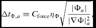
For external forces with potentials defined such that Φ → 0 as r → ∞, an additional constraint is applied using (Dehnen & Read Reference Dehnen and Read2011)
 $$\begin{equation}
\Delta t_{{\Phi },a} \equiv C_{\rm force} \eta _\Phi \sqrt{\frac{\vert \Phi _{a}\vert }{\vert \nabla \Phi \vert _{a}^{2}}},
\end{equation}$$
$$\begin{equation}
\Delta t_{{\Phi },a} \equiv C_{\rm force} \eta _\Phi \sqrt{\frac{\vert \Phi _{a}\vert }{\vert \nabla \Phi \vert _{a}^{2}}},
\end{equation}$$
where  $\eta _\Phi = 0.05$ (see Section 2.8.5).
The timestep for particle a is then taken to be the minimum of all of the above constraints, i.e.
 $$\begin{eqnarray}
\Delta t_{a} = \min & \left(\Delta t_{\rm C}, \Delta t_{\rm f}, \Delta t_{\rm ext}, \Delta t_{\rm sink-gas}, \Delta t_{\Phi } \right)_a,
\end{eqnarray}$$
$$\begin{eqnarray}
\Delta t_{a} = \min & \left(\Delta t_{\rm C}, \Delta t_{\rm f}, \Delta t_{\rm ext}, \Delta t_{\rm sink-gas}, \Delta t_{\Phi } \right)_a,
\end{eqnarray}$$
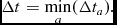
with possible other constraints arising from additional physics as described in their respective sections. With global timestepping, the resulting timestep is the minimum over all particles
 $$\begin{equation}
\Delta t = \min _{a} ( \Delta t_a).
\end{equation}$$
$$\begin{equation}
\Delta t = \min _{a} ( \Delta t_a).
\end{equation}$$
2.3.3. Substepping of external forces
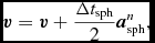
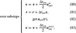
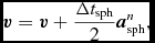
In the case where the timestep is dominated by any of the external force timesteps, i.e. (74)–(76), we implement an operator splitting approach implemented according to the reversible reference system propagator algorithm (RESPA) derived by Tuckerman, Berne, & Martyna (Reference Tuckerman, Berne and Martyna1992) for molecular dynamics. RESPA splits the acceleration into ‘long-range’ and ‘short-range’ contributions, which in Phantom are defined to be the SPH and external/point-mass accelerations, respectively.
Our implementation follows Tuckerman et al. (Reference Tuckerman, Berne and Martyna1992) (see their Appendix B), where the velocity is first predicted to the half step using the ‘long-range’ forces, followed by an inner loop where the positions are updated with the current velocity and the velocities are updated with the ‘short-range’ accelerations. Thus, the timestepping proceeds according to
 $$\begin{equation}
{\bm v} = {\bm v} + \frac{\Delta t_{\rm sph}}{2} {\bm a}_{\rm sph}^{n},\vspace*{-6pt}
\end{equation}$$
$$\begin{equation}
{\bm v} = {\bm v} + \frac{\Delta t_{\rm sph}}{2} {\bm a}_{\rm sph}^{n},\vspace*{-6pt}
\end{equation}$$
 \begin{eqnarray*}
{\rm over\ substeps}\left\{\begin{array}{rcl}
\bm v &=& {\bm v} + \displaystyle\frac{\Delta t_{\rm ext}}{2} {\bm a}_{\rm ext}^{m}, \\
{\bm r} &=& {\bm r} + \Delta t_{\rm ext} {\bm v}, \\
&&\qquad\textrm {get } {\bm a}_{\rm ext}({\bm r}),\\
{\bm v} &=& {\bm v} + \frac{\Delta t_{\rm ext}}{2} {\bm a}_{\rm ext}^{m+1},
\end{array}\right.
\end{eqnarray*}
\begin{eqnarray*}
{\rm over\ substeps}\left\{\begin{array}{rcl}
\bm v &=& {\bm v} + \displaystyle\frac{\Delta t_{\rm ext}}{2} {\bm a}_{\rm ext}^{m}, \\
{\bm r} &=& {\bm r} + \Delta t_{\rm ext} {\bm v}, \\
&&\qquad\textrm {get } {\bm a}_{\rm ext}({\bm r}),\\
{\bm v} &=& {\bm v} + \frac{\Delta t_{\rm ext}}{2} {\bm a}_{\rm ext}^{m+1},
\end{array}\right.
\end{eqnarray*}
 $$\begin{equation}
\hspace*{-15.53pt}\textrm {get } {\bm a}_{\rm sph}({\bm r}),\hspace*{15.53pt} \vspace*{-6pt}
\end{equation}$$
$$\begin{equation}
\hspace*{-15.53pt}\textrm {get } {\bm a}_{\rm sph}({\bm r}),\hspace*{15.53pt} \vspace*{-6pt}
\end{equation}$$
 $$\begin{equation}
{\bm v} = {\bm v} + \frac{\Delta t_{\rm sph}}{2} {\bm a}_{\rm sph}^{n},
\end{equation}$$
$$\begin{equation}
{\bm v} = {\bm v} + \frac{\Delta t_{\rm sph}}{2} {\bm a}_{\rm sph}^{n},
\end{equation}$$
where  ${\bm a}_{\rm sph}$ indicates the SPH acceleration evaluated from (34) and ${\bm a}_{\rm ext}$ indicates the external forces. The SPH and external accelerations are stored separately to enable this. Δt ext is the minimum of all timesteps relating to sink–gas and external forces [equations (74)–(76)], while Δt sph is the timestep relating to the SPH forces [equations (72), (73), and (288)]. Δt ext is allowed to vary on each substep, so we take as many steps as required such that ∑m − 1jΔt ext, j + Δt ext, f = Δt sph, where Δt ext, f < Δt ext, j is chosen so that the sum will identically equal Δt sph. The number of substeps is m ≈ int(Δt ext, min/Δt sph, min) + 1, where the minimum is taken over all particles.
2.3.4. Individual particle timesteps
For simulations of stiff problems with a large range in timestep over the domain, it is more efficient to allow each particle to evolve on its own timestep independently (Bate Reference Bate1995; Springel Reference Springel2005; Saitoh & Makino Reference Saitoh and Makino2010). This violates all of the conservation properties of the Leapfrog integrator [see Makino et al. (Reference Makino, Hut, Kaplan and Saygın2006) for an attempt to solve this], but can speed up the calculation by an order of magnitude or more. We implement this in the usual blockstepped manner by assigning timesteps in factor-of-two decrements from some maximum timestep Δt max, which for convenience is set equal to the time between output files.
We implement a timestep limiter where the timestep for an active particle is constrained to be within a factor of 2 of its neighbours, similar to condition employed by Saitoh & Makino (Reference Saitoh and Makino2009). Additionally, inactive particles will be woken up as required to ensure that their timestep is within a factor of 2 of its neighbours.
The practical side of individual timestepping is described in Appendix A.6.
2.4. External forces
2.4.1. Point-mass potential
The simplest external force describes a point mass, M, at the origin, which yields gravitational potential and acceleration:
 $$\begin{equation}
\Phi _{a} = -\frac{GM}{r_{a}}, \hspace{28.45274pt} {\bm a}_{{\rm ext},a} = -\nabla \Phi _{a} = -\frac{GM}{\vert {\bm r}_{a} \vert ^{3}} {\bm r}_{a},
\end{equation}$$
$$\begin{equation}
\Phi _{a} = -\frac{GM}{r_{a}}, \hspace{28.45274pt} {\bm a}_{{\rm ext},a} = -\nabla \Phi _{a} = -\frac{GM}{\vert {\bm r}_{a} \vert ^{3}} {\bm r}_{a},
\end{equation}$$
where  $r_{a} \equiv \vert {\bm r}_{a} \vert \equiv \sqrt{{\bm r}_{a}\cdot {\bm r}_{a}}$. When this potential is used, we allow for particles within a certain radius, R acc, from the origin to be accreted. This allows for a simple treatment of accretion discs where the mass of the disc is assumed to be negligible compared to the mass of the central object. The accreted mass in this case is recorded but not added to the central mass. For more massive discs, or when the accreted mass is significant with respect to the central mass, it is better to model the central star using a sink particle (Section 2.8) where there are mutual gravitational forces between the star and the disc, and any mass accreted is added to the point mass (Section 2.8.2).
2.4.2. Binary potential
We provide the option to model motion in binary systems where the mass of the disc is negligible. In this case, the binary motion is prescribed using
 $$\begin{eqnarray}
{\bm r}_{1} = [(1 - M) \cos (t),(1- M) \sin (t), 0],
\end{eqnarray}$$
$$\begin{eqnarray}
{\bm r}_{1} = [(1 - M) \cos (t),(1- M) \sin (t), 0],
\end{eqnarray}$$
 $$\begin{eqnarray}
{\bm r}_{2} = [- M \cos (t), - M \sin (t), 0],
\end{eqnarray}$$
$$\begin{eqnarray}
{\bm r}_{2} = [- M \cos (t), - M \sin (t), 0],
\end{eqnarray}$$
where M is the mass ratio in units of the total mass (which is therefore unity). For this potential, G and Ω are set to unity in computational units, where Ω is the angular velocity of the binary. Thus, only M needs to be specified to fix both m 1 and m 2. Hence, the binary remains fixed on a circular orbit at r = 1. The binary potential is therefore
 $$\begin{equation}
\Phi _{a} = -\frac{M}{\vert {\bm r}_{a} - {\bm r}_{1} \vert } - \frac{(1- M) }{\vert {\bm r}_{a} - {\bm r}_{2} \vert },
\end{equation}$$
$$\begin{equation}
\Phi _{a} = -\frac{M}{\vert {\bm r}_{a} - {\bm r}_{1} \vert } - \frac{(1- M) }{\vert {\bm r}_{a} - {\bm r}_{2} \vert },
\end{equation}$$
such that the external acceleration is given by
 $$\begin{equation}
{\bm a}_{{\rm ext},a} = -\nabla \Phi _{a} = - M \frac{({\bm r}_{a} - {\bm r}_{1})}{\vert {\bm r}_{a} - {\bm r}_{1} \vert ^3} - (1- M) \frac{({\bm r}_{a} - {\bm r}_{2})}{\vert {\bm r}_{a} - {\bm r}_{2} \vert ^3}.
\end{equation}$$
$$\begin{equation}
{\bm a}_{{\rm ext},a} = -\nabla \Phi _{a} = - M \frac{({\bm r}_{a} - {\bm r}_{1})}{\vert {\bm r}_{a} - {\bm r}_{1} \vert ^3} - (1- M) \frac{({\bm r}_{a} - {\bm r}_{2})}{\vert {\bm r}_{a} - {\bm r}_{2} \vert ^3}.
\end{equation}$$
Again, there is an option to accrete particles that fall within a certain radius from either star (R acc, 1 or R acc, 2, respectively). For most binary accretion disc simulations (e.g. planet migration), it is better to use ‘live’ sink particles to represent the binary so that there is feedback between the binary and the disc (we have used a live binary in all of our simulations to date, e.g. Nixon, King, & Price Reference Nixon, King and Price2013; Facchini, Lodato, & Price Reference Facchini, Lodato and Price2013; Martin et al. Reference Martin, Nixon, Armitage, Lubow and Price2014a, Reference Martin, Nixon, Lubow, Armitage, Price, Doğan and King2014b; Doğan et al. Reference Doğan, Nixon, King and Price2015; Ragusa, Lodato, & Price Reference Ragusa, Lodato and Price2016; Ragusa et al. Reference Ragusa, Dipierro, Lodato, Laibe and Price2017), but the binary potential remains useful under limited circumstances—in particular, when one wishes to turn off the feedback between the disc and the binary.
Given that the binary potential is time-dependent, for efficiency, we compute the position of the binary only once at the start of each timestep, and use these stored positions to compute the accelerations of the SPH particles via (90).
2.4.3. Binary potential with gravitational wave decay
An alternative binary potential including the effects of gravitational wave decay was used by Cerioli, Lodato, & Price (Reference Cerioli, Lodato and Price2016) to study the squeezing of discs during the merger of supermassive black holes. Here the motion of the binary is prescribed according to
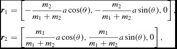 $$\begin{eqnarray}
{\bm r}_{1} & =& \left[-\frac{m_{2}}{m_{1} + m_{2}} a \cos (\theta ), -\frac{m_{2}}{m_{1} + m_{2}} a \sin (\theta ), 0 \right], \nonumber \\
{\bm r}_{2} & =& \left[\frac{m_{1}}{m_{1} + m_{2}} a \cos (\theta ), \frac{m_{1}}{m_{1} + m_{2}} a \sin (\theta ), 0 \right],
\end{eqnarray}$$
$$\begin{eqnarray}
{\bm r}_{1} & =& \left[-\frac{m_{2}}{m_{1} + m_{2}} a \cos (\theta ), -\frac{m_{2}}{m_{1} + m_{2}} a \sin (\theta ), 0 \right], \nonumber \\
{\bm r}_{2} & =& \left[\frac{m_{1}}{m_{1} + m_{2}} a \cos (\theta ), \frac{m_{1}}{m_{1} + m_{2}} a \sin (\theta ), 0 \right],
\end{eqnarray}$$
where the semi-major axis, a, decays according to
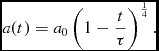 $$\begin{equation}
a(t) = a_{0} \left(1 - \frac{t}{\tau } \right)^{\frac{1}{4}} .
\end{equation}$$
$$\begin{equation}
a(t) = a_{0} \left(1 - \frac{t}{\tau } \right)^{\frac{1}{4}} .
\end{equation}$$
The initial separation is a 0, with τ defined as the time to merger, given by the usual expression (e.g. Lodato et al. Reference Lodato, Nayakshin, King and Pringle2009)
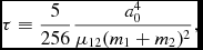 $$\begin{equation}
\tau \equiv \frac{5}{256} \frac{a_{0}^{4}}{\mu _{12} (m_{1} + m_{2})^{2}},
\end{equation}$$
$$\begin{equation}
\tau \equiv \frac{5}{256} \frac{a_{0}^{4}}{\mu _{12} (m_{1} + m_{2})^{2}},
\end{equation}$$
where
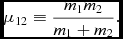 $$\begin{equation}
\mu _{12} \equiv \frac{m_1 m_2}{m_1 + m_2}.
\end{equation}$$
$$\begin{equation}
\mu _{12} \equiv \frac{m_1 m_2}{m_1 + m_2}.
\end{equation}$$
The angle θ is defined using
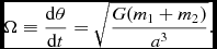 $$\begin{equation}
\Omega \equiv \frac{{\rm d}\theta }{{\rm d}t} = \sqrt{\frac{G(m_{1} + m_{2})}{a^{3}}}.
\end{equation}$$
$$\begin{equation}
\Omega \equiv \frac{{\rm d}\theta }{{\rm d}t} = \sqrt{\frac{G(m_{1} + m_{2})}{a^{3}}}.
\end{equation}$$
Inserting the expression for a and integrating gives (Cerioli et al. Reference Cerioli, Lodato and Price2016)
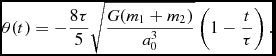 $$\begin{equation}
\theta (t) = -\frac{8\tau }{5} \sqrt{\frac{G(m_{1} + m_{2})}{a_{0}^{3}}} \left( 1 - \frac{t}{\tau } \right).
\end{equation}$$
$$\begin{equation}
\theta (t) = -\frac{8\tau }{5} \sqrt{\frac{G(m_{1} + m_{2})}{a_{0}^{3}}} \left( 1 - \frac{t}{\tau } \right).
\end{equation}$$
The positions of the binary,  ${\bm r}_1$ and ${\bm r}_2$, can be inserted into (89) to obtain the binary potential, with the acceleration as given in (90). The above can be used as a simple example of a time-dependent external potential.
2.4.4. Galactic potentials
We implement a range of external forces representing various galactic potentials, as used in Pettitt et al. (Reference Pettitt, Dobbs, Acreman and Price2014). These include arm, bar, halo, disc, and spheroidal components. We refer the reader to the paper above for the actual forms of the potentials.
For the non-axisymmetric potentials, a few important parameters that determine the morphology can be changed at run time rather than compile time. These include the pattern speed, arm number, arm pitch angle, and bar axis lengths (where applicable). In the case of non-axisymmetric components, the user should be aware that some will add mass to the system, whereas others simply perturb the galactic disc. These potentials can be used for any galactic system, but the various default scale lengths and masses are chosen to match the Milky Way’s rotation curve (Sofue Reference Sofue2012).
The most basic potential in Phantom is a simple logarithmic potential from Binney & Tremaine (Reference Binney and Tremaine1987), which allows for the reproduction of a purely flat rotation curve with steep decrease at the galactic centre, and approximates the halo, bulge, and disc contributions. Also included is the standard flattened disc potential of Miyamoto–Nagai (Miyamoto & Nagai Reference Miyamoto and Nagai1975) and an exponential profile disc, specifically the form from Khoperskov et al. (Reference Khoperskov, Vasiliev, Sobolev and Khoperskov2013). Several spheroidal components are available, including the potentials of Plummer (Reference Plummer1911), Hernquist (Reference Hernquist1990), and Hubble (Reference Hubble1930). These can be used generally for bulges and halos if given suitable mass and scale lengths. We also include a few halo-specific profiles; the NFW (Navarro, Frenk, & White Reference Navarro, Frenk and White1996), Begeman, Broeils, & Sanders (Reference Begeman, Broeils and Sanders1991), Caldwell & Ostriker (Reference Caldwell and Ostriker1981), and the Allen & Santillan (Reference Allen and Santillan1991) potentials.
The arm potentials include some of the more complicated profiles. The first is the potential of Cox & Gómez (Reference Cox and Gómez2002), which is a relatively straightforward superposition of three sinusoidal-based spiral components to damp the potential ‘troughs’ in the inter-arm minima. The other spiral potential is from Pichardo et al. (Reference Pichardo, Martos, Moreno and Espresate2003), and is more complicated. Here, the arms are constructed from a superposition of oblate spheroids whose loci are placed along a standard logarithmic spiral. As the force from this potential is computationally expensive it is prudent to pre-compute a grid of potential/force and read it at run time. The python code to generate the appropriate grid files is distributed with the code.
Finally, the bar components: We include the bar potentials of Dehnen (Reference Dehnen2000a), Wada & Koda (Reference Wada and Koda2001), the ‘S’ shaped bar of Vogt & Letelier (Reference Vogt and Letelier2011), both biaxial and triaxial versions provided in Long & Murali (Reference Long and Murali1992), and the boxy-bulge bar of Wang et al. (Reference Wang, Zhao, Mao and Rich2012). This final bar contains both a small inner non-axisymmetric bulge and longer bar component, with the forces calculated by use of Hernquist–Ostriker expansion coefficients of the bar density field. Phantom contains the coefficients for several different forms of this bar potential.
2.4.5. Lense–Thirring precession
Lense–Thirring precession (Lense & Thirring Reference Lense and Thirring1918) from a spinning black hole is implemented in a post-Newtonian approximation following Nelson & Papaloizou (Reference Nelson and Papaloizou2000), which has been used in Nixon et al. (Reference Nixon, King, Price and Frank2012b), Nealon, Price, & Nixon (Reference Nealon, Price and Nixon2015), and Nealon et al. (Reference Nealon, Nixon, Price and King2016). In this case, the external acceleration consists of a point-mass potential (Section 2.4.1) and the Lense–Thirring term:
 $$\begin{equation}
{\bm a}_{{\rm ext},a} = -\nabla \Phi _a + {\bm v}_a \times {\bm \Omega }_{p,a},
\end{equation}$$
$$\begin{equation}
{\bm a}_{{\rm ext},a} = -\nabla \Phi _a + {\bm v}_a \times {\bm \Omega }_{p,a},
\end{equation}$$
where Φa is given by (86) and  ${\bm v}_a \times {\bm \Omega }_{p,a}$ is the gravitomagnetic acceleration. A dipole approximation is used, yielding
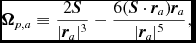 $$\begin{equation}
{\bm \Omega }_{p,a} \equiv \frac{2{\bm S}}{\vert {\bm r}_a \vert ^{3}} - \frac{6({\bm S}\cdot {\bm r}_a) {\bm r}_a}{\vert {\bm r}_a \vert ^{5}},
\end{equation}$$
$$\begin{equation}
{\bm \Omega }_{p,a} \equiv \frac{2{\bm S}}{\vert {\bm r}_a \vert ^{3}} - \frac{6({\bm S}\cdot {\bm r}_a) {\bm r}_a}{\vert {\bm r}_a \vert ^{5}},
\end{equation}$$
with  ${\bm S} = a_{\rm spin} (GM)^{2} {\bm k}/c^{3}$, where ${\bm k}$ is a unit vector in the direction of the black hole spin. When using the Lense–Thirring force, geometric units are assumed such that G = M = c = 1, as described in Section 2.2.3, but with the additional constraints on the unit system from M and c.
Since in this case the external force depends on velocity, it cannot be implemented directly into Leapfrog. The method we employ to achieve this is simpler than those proposed elsewhere [c.f. attempts by Quinn et al. (Reference Quinn, Perrine, Richardson and Barnes2010) and Rein & Tremaine (Reference Rein and Tremaine2011) to adapt the Leapfrog integrator to Hill’s equations]. Our approach is to split the acceleration into position and velocity-dependent parts, i.e.
 $$\begin{equation}
{\bm a}_{\rm ext} = {\bm a}_{\rm ext,x}({\bm r}) + {\bm a}_{\rm ext,v}({\bm r}, {\bm v}).
\end{equation}$$
$$\begin{equation}
{\bm a}_{\rm ext} = {\bm a}_{\rm ext,x}({\bm r}) + {\bm a}_{\rm ext,v}({\bm r}, {\bm v}).
\end{equation}$$
The position-dependent part [i.e.  $-\nabla \Phi ({\bm r})$] is integrated as normal. The velocity-dependent Lense–Thirring term is added to the predictor step, (66)–(67), as usual, but the corrector step, (69), is written in the form
 $$\begin{equation}
{\bm v}^{n + 1} = {\bm v}^{n + \frac{1}{2}} + \frac{1}{2} \Delta t \left[ {\bm a}_{\rm sph}^{n+1} + {\bm a}_{\rm ext,x}^{n+1} + {\bm a}_{\rm ext,v}({\bm r}^{n+1}, {\bm v}^{n+1})\right],
\end{equation}$$
$$\begin{equation}
{\bm v}^{n + 1} = {\bm v}^{n + \frac{1}{2}} + \frac{1}{2} \Delta t \left[ {\bm a}_{\rm sph}^{n+1} + {\bm a}_{\rm ext,x}^{n+1} + {\bm a}_{\rm ext,v}({\bm r}^{n+1}, {\bm v}^{n+1})\right],
\end{equation}$$
where  ${\bm v}^{n + \frac{1}{2}} \equiv {\bm v}^{n} + \frac{1}{2} \Delta t {\bm a}^{n}$ as in (65). This equation is implicit but the trick is to notice that it can be solved analytically for simple forcesFootnote 4. In the case of Lense–Thirring precession, we have
 $$\begin{equation}
{\bm v}^{n + 1} = \tilde{\bm v} + \frac{1}{2} \Delta t \left[{\bm v}^{n+1} \times {\bm \Omega }_{p}({\bm r}^{n+1}) \right],
\end{equation}$$
$$\begin{equation}
{\bm v}^{n + 1} = \tilde{\bm v} + \frac{1}{2} \Delta t \left[{\bm v}^{n+1} \times {\bm \Omega }_{p}({\bm r}^{n+1}) \right],
\end{equation}$$
where  $\tilde{\bm v} \equiv {\bm v}^{n + \frac{1}{2}} + \frac{1}{2} \Delta t ({\bm a}_{\rm sph}^{n+1} + {\bm a}_{\rm ext,x}^{n+1})$. We therefore have a matrix equation in the form
 $$\begin{equation}
{\bm R} {\bm v}^{n+1} = \tilde{\bm v},
\end{equation}$$
$$\begin{equation}
{\bm R} {\bm v}^{n+1} = \tilde{\bm v},
\end{equation}$$
where  ${\bm R}$ is the 3 × 3 matrix given by
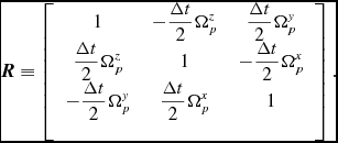 $$\begin{equation}
{\bm R} \equiv \left[ \arraycolsep5pt\begin{array}{ccc}1 & - \displaystyle\frac{\Delta t}{2} \Omega ^{z}_{p} & \displaystyle\frac{\Delta t}{2} \Omega ^{y}_{p} \\[3pt]
\displaystyle\frac{\Delta t}{2} \Omega ^{z}_{p} & 1 & -\displaystyle\frac{\Delta t}{2} \Omega ^{x}_{p} \\[3pt]
-\displaystyle\frac{\Delta t}{2} \Omega ^{y}_{p} & \displaystyle\frac{\Delta t}{2} \Omega ^{x}_{p} & 1 \\
\end{array} \right].
\end{equation}$$
$$\begin{equation}
{\bm R} \equiv \left[ \arraycolsep5pt\begin{array}{ccc}1 & - \displaystyle\frac{\Delta t}{2} \Omega ^{z}_{p} & \displaystyle\frac{\Delta t}{2} \Omega ^{y}_{p} \\[3pt]
\displaystyle\frac{\Delta t}{2} \Omega ^{z}_{p} & 1 & -\displaystyle\frac{\Delta t}{2} \Omega ^{x}_{p} \\[3pt]
-\displaystyle\frac{\Delta t}{2} \Omega ^{y}_{p} & \displaystyle\frac{\Delta t}{2} \Omega ^{x}_{p} & 1 \\
\end{array} \right].
\end{equation}$$
Rearranging (102),  ${\bm v}^{n+1}$ is obtained by using
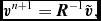 $$\begin{equation}
{\bm v}^{n+1} = {\bm R}^{-1}\tilde{\bm v},
\end{equation}$$
$$\begin{equation}
{\bm v}^{n+1} = {\bm R}^{-1}\tilde{\bm v},
\end{equation}$$
where  ${\bm R}^{-1}$ is the inverse of ${\bm R}$, which we invert using the analytic solution.
2.4.6. Generalised Newtonian potential
The generalised Newtonian potential described by Tejeda & Rosswog (Reference Tejeda and Rosswog2013) is implemented, where the acceleration terms are given by
 $$\begin{equation}
{\bm a}_{{\rm ext},a} = -\frac{GM{\bm r}_a}{\vert {\bm r}_a \vert ^{3}}f^{2} + \frac{2R_{\rm g} {\bm v}_a ({\bm v}_a \cdot {\bm r}_a)}{\vert {\bm r}_a \vert ^{3} f} - \frac{3 R_{\rm g} {\bm r}_a ({\bm v}_a \times {\bm r}_a)^{2}}{\vert {\bm r}_a \vert ^{5}},
\end{equation}$$
$$\begin{equation}
{\bm a}_{{\rm ext},a} = -\frac{GM{\bm r}_a}{\vert {\bm r}_a \vert ^{3}}f^{2} + \frac{2R_{\rm g} {\bm v}_a ({\bm v}_a \cdot {\bm r}_a)}{\vert {\bm r}_a \vert ^{3} f} - \frac{3 R_{\rm g} {\bm r}_a ({\bm v}_a \times {\bm r}_a)^{2}}{\vert {\bm r}_a \vert ^{5}},
\end{equation}$$
with R g ≡ GM/c 3 and  $f \equiv \left(1 - 2R_{\rm g}/\vert {\bm r}_a \vert \right)$. See Bonnerot et al. (Reference Bonnerot, Rossi, Lodato and Price2016) for a recent application. This potential reproduces several features of the Schwarzschild (Reference Schwarzschild1916) spacetime, in particular, reproducing the orbital and epicyclic frequencies to better than 7% (Tejeda & Rosswog Reference Tejeda and Rosswog2013). As the acceleration involves velocity-dependent terms, it requires a semi-implicit solution like Lense–Thirring precession. Since the matrix equation is rather involved for this case, the corrector step is iterated using fixed point iterations until the velocity of each particle is converged to a tolerance of 1%.
2.4.7. Poynting–Robertson drag
The radiation drag from a central point-like, gravitating, radiating, and non-rotating object may be applied as an external force. The implementation is intended to be as general as possible. The acceleration of a particle subject to these external forces is
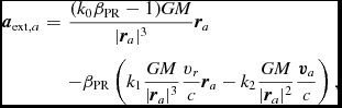 $$\begin{eqnarray}
{\bm a}_{{\rm ext},a} &=& \frac{(k_0\beta _{\rm PR}-1)GM}{\vert {\bm r}_a \vert ^3} \bm r_a \nonumber \\
&& -\beta _{\rm PR} \left(k_1\frac{GM}{\vert {\bm r}_a \vert ^3}\frac{v_r}{c}\bm r_a -k_2\frac{GM}{\vert {\bm r}_a \vert ^2}\frac{\bm v_a}{c}\right),
\end{eqnarray}$$
$$\begin{eqnarray}
{\bm a}_{{\rm ext},a} &=& \frac{(k_0\beta _{\rm PR}-1)GM}{\vert {\bm r}_a \vert ^3} \bm r_a \nonumber \\
&& -\beta _{\rm PR} \left(k_1\frac{GM}{\vert {\bm r}_a \vert ^3}\frac{v_r}{c}\bm r_a -k_2\frac{GM}{\vert {\bm r}_a \vert ^2}\frac{\bm v_a}{c}\right),
\end{eqnarray}$$
where v r is the component of the velocity in the radial direction. The parameter βPR is the ratio of radiation to gravitational forces, supplied by a separate user-written module. Relativistic effects are neglected because these are thought to be less important than radiation forces for low (βPR < 0.01) luminosities, even in accreting neutron star systems where a strong gravitational field is present (e.g., Miller & Lamb Reference Miller and Lamb1993).
The three terms on the right side of (106) correspond, respectively, to gravity (reduced by outward radiation pressure), redshift-related modification to radiation pressure caused by radial motion, and Poynting–Robertson drag against the direction of motion. These three terms can be scaled independently by changing the three parameters k 0, k 1, and k 2, whose default values are unity. Rotation of the central object can be crudely emulated by changing k 2.
As for Lense–Thirring precession, the  ${\bm a}^{n+1}$ term of the Leapfrog integration scheme can be expanded into velocity-dependent and non-velocity-dependent component. We obtain, after some algebra,
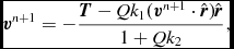 $$\begin{equation}
\bm v^{n+1} =-\frac{\bm T-Qk_1(\bm v^{n+1}\cdot \hat{\bm r})\hat{\bm r}}{1+Qk_2},
\end{equation}$$
$$\begin{equation}
\bm v^{n+1} =-\frac{\bm T-Qk_1(\bm v^{n+1}\cdot \hat{\bm r})\hat{\bm r}}{1+Qk_2},
\end{equation}$$
where
 $$\begin{equation}
\bm T=\bm v^n+\frac{1}{2}\Delta t\bm a^n-\frac{(1-k_0\beta _{\rm PR})GM\Delta t}{2r^3}\bm r
\end{equation}$$
$$\begin{equation}
\bm T=\bm v^n+\frac{1}{2}\Delta t\bm a^n-\frac{(1-k_0\beta _{\rm PR})GM\Delta t}{2r^3}\bm r
\end{equation}$$
and
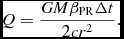 $$\begin{equation}
Q=\frac{GM\beta _{\rm PR}\Delta t}{2cr^2}.
\end{equation}$$
$$\begin{equation}
Q=\frac{GM\beta _{\rm PR}\Delta t}{2cr^2}.
\end{equation}$$
Equation (107) yields a set of simultaneous equations for the three vector components that can be solved analytically. A detailed derivation is given in Worpel (Reference Worpel2015).
2.4.8. Coriolis and centrifugal forces
Under certain circumstances, it is useful to perform calculations in a co-rotating reference frame (e.g. for damping binary stars into equilibrium with each other). The resulting acceleration terms are given by
 $$\begin{equation}
{\bm a}_{{\rm ext},a} = -{\bm \Omega } \times ({\bm \Omega } \times {\bm r}_a) - 2 ({\bm \Omega } \times {\bm v}_a),
\end{equation}$$
$$\begin{equation}
{\bm a}_{{\rm ext},a} = -{\bm \Omega } \times ({\bm \Omega } \times {\bm r}_a) - 2 ({\bm \Omega } \times {\bm v}_a),
\end{equation}$$
which are the centrifugal and Coriolis terms, respectively, with  ${\bm \Omega }$ the angular rotation vector. The timestepping algorithm is as described above for Lense–Thirring precession, with the velocity-dependent term handled by solving the 3 × 3 matrix in the Leapfrog corrector step.
2.5. Driven turbulence
Phantom implements turbulence driving in periodic domains via an Ornstein–Uhlenbeck stochastic driving of the acceleration field, as first suggested by Eswaran & Pope (Reference Eswaran and Pope1988). This is an SPH adaptation of the module used in the grid-based simulations by Schmidt, Hillebrandt, & Niemeyer (Reference Schmidt, Hillebrandt and Niemeyer2006) and Federrath, Klessen, & Schmidt (Reference Federrath, Klessen and Schmidt2008) and many subsequent works. This module was first used in Phantom by Price & Federrath (Reference Price and Federrath2010) to compare the statistics of isothermal, supersonic turbulence between SPH, and grid methods. Subsequent applications have been to the density variance–Mach number relation (Price et al. Reference Price, Federrath and Brunt2011), subsonic turbulence (Price Reference Price2012b), supersonic MHD turbulence (Tricco et al. Reference Tricco, Price and Federrath2016b), and supersonic turbulence in a dust–gas mixture (Tricco et al. Reference Tricco, Price and Laibe2017). Adaptations of this module have also been incorporated into other SPH codes (Bauer & Springel Reference Bauer and Springel2012; Valdarnini Reference Valdarnini2016).
The amplitude and phase of each Fourier mode is initialised by creating a set of six random numbers, z n, drawn from a random Gaussian distribution with unit variance. These are generated by the usual Box–Muller transformation (e.g. Press et al. Reference Press, Teukolsky, Vetterling and Flannery1992) by selecting two uniform random deviates u 1, u 2 ∈ [0, 1] and constructing the amplitude according to
 $$\begin{equation}
z = \sqrt{2 \log (1 /u_{1})} \cos (2 \pi u_{2}).
\end{equation}$$
$$\begin{equation}
z = \sqrt{2 \log (1 /u_{1})} \cos (2 \pi u_{2}).
\end{equation}$$
The six Gaussian random numbers are set up according to
 $$\begin{equation}
{\bm x}_{n} = \sigma {\bm z}_{n},
\end{equation}$$
$$\begin{equation}
{\bm x}_{n} = \sigma {\bm z}_{n},
\end{equation}$$
where the standard deviation, σ, is set to the square root of the energy per mode divided by the correlation time,  $\sigma = \sqrt{E_{\rm m}/t_{\rm decay}}$, where both E m and t decay are user-specified parameters.
The ‘red noise’ sequence (Uhlenbeck & Ornstein Reference Uhlenbeck and Ornstein1930) is generated for each mode at each timestep according to (Bartosch Reference Bartosch2001)
 $$\begin{equation}
{\bm x}_{n+1}= f {\bm x}_{n} + \sigma \sqrt{(1 - f^{2})} {\bm z}_n,
\end{equation}$$
$$\begin{equation}
{\bm x}_{n+1}= f {\bm x}_{n} + \sigma \sqrt{(1 - f^{2})} {\bm z}_n,
\end{equation}$$
where f = exp(− Δt/t decay) is the damping factor. The resulting sequence has zero mean with root-mean-square equal to the variance. The power spectrum in the time domain can vary from white noise [P(f) constant] to ‘brown noise’ [P(f) = 1/f 2].
The amplitudes and phases of each mode are constructed by splitting  ${\bm x}_{n}$ into two vectors, ${\bm \Phi }_{a}$ and ${\bm \Phi }_{b}$ of length 3, employed to construct divergence- and curl-free fields according to
 $$\begin{eqnarray}
{\bm A}_{m} = w [{\bm \Phi }_{a} - ( {\bm \Phi }_{a} \cdot \hat{\bm k} )\hat{\bm k}] + (1 - w)[({\bm \Phi }_{b} \cdot \hat{\bm k} )\hat{\bm k}] ,
\end{eqnarray}$$\vspace*{-15pt}
$$\begin{eqnarray}
{\bm A}_{m} = w [{\bm \Phi }_{a} - ( {\bm \Phi }_{a} \cdot \hat{\bm k} )\hat{\bm k}] + (1 - w)[({\bm \Phi }_{b} \cdot \hat{\bm k} )\hat{\bm k}] ,
\end{eqnarray}$$\vspace*{-15pt}
 $$\begin{eqnarray}
{\bm B}_{m} = w [{\bm \Phi }_{b} - ( {\bm \Phi }_{b} \cdot \hat{\bm k} )\hat{\bm k}] + (1 - w)[({\bm \Phi }_{a} \cdot \hat{\bm k} )\hat{\bm k}] ,
\end{eqnarray}$$
$$\begin{eqnarray}
{\bm B}_{m} = w [{\bm \Phi }_{b} - ( {\bm \Phi }_{b} \cdot \hat{\bm k} )\hat{\bm k}] + (1 - w)[({\bm \Phi }_{a} \cdot \hat{\bm k} )\hat{\bm k}] ,
\end{eqnarray}$$
where  ${\bm k} = [k_{x}, k_{y}, k_{z}]$ is the mode frequency. The parameter w ∈ [0, 1] is the ‘solenoidal weight’, specifying whether the driving should be purely solenoidal (w = 1) or purely compressive (w = 0) (see Federrath et al. Reference Federrath, Klessen and Schmidt2008, Reference Federrath, Roman-Duval, Klessen, Schmidt and Mac Low2010a).
The spectral form of the driving is defined in Fourier space, with options for three possible spectral forms
 $$\begin{equation}
C_{m} = \left\lbrace \arraycolsep5pt\begin{array}{@{}ll@{}}1 & \textrm {uniform} \\[6pt]
4 (a_{\rm min} - 1) \displaystyle\frac{(k - k_{c})^{2}}{(k_{\max } - k_{\min })^{2}} + 1 & \textrm {parabolic} \\[3pt]
k/k_{\min }^{-5/3} & \textrm {Kolmogorov,} \end{array}\right.
\end{equation}$$
$$\begin{equation}
C_{m} = \left\lbrace \arraycolsep5pt\begin{array}{@{}ll@{}}1 & \textrm {uniform} \\[6pt]
4 (a_{\rm min} - 1) \displaystyle\frac{(k - k_{c})^{2}}{(k_{\max } - k_{\min })^{2}} + 1 & \textrm {parabolic} \\[3pt]
k/k_{\min }^{-5/3} & \textrm {Kolmogorov,} \end{array}\right.
\end{equation}$$
where 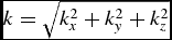 $k = \sqrt{k_{x}^{2} + k_{y}^{2} + k_{z}^{2}}$ is the wavenumber, with non-zero amplitudes defined only for wavenumbers where k min ⩽ k ⩽ k max, and a min is the amplitude of the modes at k min and k max in the parabolic case (we use a min = 0 in the code). The frequency grid is defined using frequencies from k x = n x2π/L x in the x direction, where n x ∈ [0, 20] is an integer and L x is the box size in the x-direction, while k y = n y2π/L y and k z = n z2π/L z with n y ∈ [0, 8] and n z ∈ [0, 8]. We then set up four modes for each combination of n x, n y, and n z, corresponding to [k x, k y, k z], [k x, −k y, k z], [k x, k y, −k z], and [k x, −k y, −k z]. That is, we effectively sum from [− (N − 1)/2, (N − 1)/2] in the k y and k z directions in the discrete Fourier transform, where N = max(n x) is the number of frequencies. The default values for k min and k max are 2π and 6π, respectively, corresponding to large-scale driving of only the first few Fourier modes, so with default settings there are 112 non-zero Fourier modes. The maximum number of modes, defining the array sizes needed to store the stirring information, is currently set to 1,000.
We apply the forcing to the particles by computing the discrete Fourier transform over the stirring modes directly, i.e.
 $$\begin{equation}
{\bm a}_{{\rm forcing}, a} = f_{\rm sol} \sum _{m=1}^{n_{\rm modes}} C_{m} \left[ {\bm A}_{m} \cos ({\bm k}\cdot {\bm r}_{a}) - {\bm B}_{m}\sin ({\bm k}\cdot {\bm r}_{a}) \right],
\end{equation}$$
$$\begin{equation}
{\bm a}_{{\rm forcing}, a} = f_{\rm sol} \sum _{m=1}^{n_{\rm modes}} C_{m} \left[ {\bm A}_{m} \cos ({\bm k}\cdot {\bm r}_{a}) - {\bm B}_{m}\sin ({\bm k}\cdot {\bm r}_{a}) \right],
\end{equation}$$
where the factor f sol is defined from the solenoidal weight, w, according to
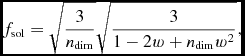 $$\begin{equation}
f_{\rm sol} = \sqrt{\frac{3}{n_{\rm dim}}} \sqrt{ \frac{3}{1 - 2w + n_{\rm dim} w^{2}}},
\end{equation}$$
$$\begin{equation}
f_{\rm sol} = \sqrt{\frac{3}{n_{\rm dim}}} \sqrt{ \frac{3}{1 - 2w + n_{\rm dim} w^{2}}},
\end{equation}$$
such that the rms acceleration is the same irrespective of the value of w. We default to purely solenoidal forcing (w = 1), with the factor f sol thus equal to  $\sqrt{3/2}$ by default. For individual timesteps, we update the driving force only when a particle is active.
To aid reproducibility, it is often desirable to pre-generate the entire driving sequence prior to performing a calculation, which can then be written to a file and read back at runtime. This was the procedure used in Price & Federrath (Reference Price and Federrath2010), Tricco et al. (Reference Tricco, Price and Federrath2016b), and Tricco et al. (Reference Tricco, Price and Laibe2017).
2.6. Accretion disc viscosity
Accretion disc viscosity is implemented in Phantom via two different approaches, as described by Lodato & Price (Reference Lodato and Price2010).
2.6.1. Disc viscosity using the shock viscosity term
The default approach is to adapt the shock viscosity term to represent a Shakura & Sunyaev (Reference Shakura and Sunyaev1973) α-viscosity, as originally proposed by Artymowicz & Lubow (Reference Artymowicz and Lubow1994) and Murray (Reference Murray1996). The key is to note that (39) and (40) represent a Navier–Stokes viscosity term with a fixed ratio between the bulk and shear viscosity terms (e.g. Murray Reference Murray1996; Jubelgas, Springel, & Dolag Reference Jubelgas, Springel and Dolag2004; Lodato & Price Reference Lodato and Price2010; Price Reference Price2012b; Meru & Bate Reference Meru and Bate2012). In particular, it can be shown (e.g. Español & Revenga Reference Español and Revenga2003) that
 $$\begin{equation}
\sum _{b} \frac{m_{b}}{\overline{\rho }_{ab}} ({\bm v}_{ab}\cdot \hat{\bm r}_{ab} )\frac{\nabla _{a} W_{ab}}{\vert r_{ab}\vert } \approx \frac{1}{5} \nabla \left( \nabla \cdot {\bm v}\right) + \frac{1}{10}\nabla ^{2} {\bm v},
\end{equation}$$
$$\begin{equation}
\sum _{b} \frac{m_{b}}{\overline{\rho }_{ab}} ({\bm v}_{ab}\cdot \hat{\bm r}_{ab} )\frac{\nabla _{a} W_{ab}}{\vert r_{ab}\vert } \approx \frac{1}{5} \nabla \left( \nabla \cdot {\bm v}\right) + \frac{1}{10}\nabla ^{2} {\bm v},
\end{equation}$$
where  $\overline{\rho }_{ab}$ is some appropriate average of the density. This enables the artificial viscosity term, (39), to be translated into the equivalent Navier–Stokes terms. In order for the artificial viscosity to represent a disc viscosity, we make the following modifications (Lodato & Price Reference Lodato and Price2010):
1. The viscosity term is applied for both approaching and receding particles.
2. The speed v sig is set equal to c s.
3. A constant αAV is adopted, turning off shock detection switches (Section 2.2.9).
4. The viscosity term is multiplied by a factor h/|r ab|.
The net result is that (40) becomes
 $$\begin{equation}
q^{a}_{ab} = \left\lbrace \arraycolsep5pt\begin{array}{@{}ll@{}}-
\displaystyle\frac{\rho _{a} h_{a}}{2 \vert r_{ab}\vert } \left(\alpha ^{\rm AV} c_{{\rm s}, a} + \beta _{\rm AV} \vert {\bm v}_{ab} \cdot \hat{\bm r}_{ab}\vert \right) {\bm v}_{ab} \cdot \hat{\bm r}_{ab}, & {\bm v}_{ab} \cdot \hat{\bm r}_{ab} < 0 \\[3pt]
- \frac{\rho _{a} h_{a}}{2 \vert r_{ab}\vert } \alpha ^{\rm AV} c_{{\rm s}, a} {\bm v}_{ab} \cdot \hat{\bm r}_{ab}. & \text{otherwise.} \end{array}\right.
\end{equation}$$
$$\begin{equation}
q^{a}_{ab} = \left\lbrace \arraycolsep5pt\begin{array}{@{}ll@{}}-
\displaystyle\frac{\rho _{a} h_{a}}{2 \vert r_{ab}\vert } \left(\alpha ^{\rm AV} c_{{\rm s}, a} + \beta _{\rm AV} \vert {\bm v}_{ab} \cdot \hat{\bm r}_{ab}\vert \right) {\bm v}_{ab} \cdot \hat{\bm r}_{ab}, & {\bm v}_{ab} \cdot \hat{\bm r}_{ab} < 0 \\[3pt]
- \frac{\rho _{a} h_{a}}{2 \vert r_{ab}\vert } \alpha ^{\rm AV} c_{{\rm s}, a} {\bm v}_{ab} \cdot \hat{\bm r}_{ab}. & \text{otherwise.} \end{array}\right.
\end{equation}$$
With the above modifications, the shear and bulk coefficients can be translated using (119) to give (e.g. Monaghan Reference Monaghan2005; Lodato & Price Reference Lodato and Price2010; Meru & Bate Reference Meru and Bate2012)
 $$\begin{eqnarray}
\nu _{\rm AV} \approx \frac{1}{10} \alpha ^{\rm AV} c_{\rm s} h,
\end{eqnarray}$$
$$\begin{eqnarray}
\nu _{\rm AV} \approx \frac{1}{10} \alpha ^{\rm AV} c_{\rm s} h,
\end{eqnarray}$$
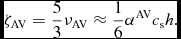 $$\begin{eqnarray}
\zeta _{\rm AV} = \frac{5}{3} \nu _{\rm AV} \approx \frac{1}{6} \alpha ^{\rm AV} c_{\rm s} h.
\end{eqnarray}$$
$$\begin{eqnarray}
\zeta _{\rm AV} = \frac{5}{3} \nu _{\rm AV} \approx \frac{1}{6} \alpha ^{\rm AV} c_{\rm s} h.
\end{eqnarray}$$
The Shakura–Sunyaev prescription is
 $$\begin{equation}
\nu = \alpha _{\rm SS} c_{\rm s} H,
\end{equation}$$
$$\begin{equation}
\nu = \alpha _{\rm SS} c_{\rm s} H,
\end{equation}$$
where H is the scale height. This implies that αSS may be determined from αAV using
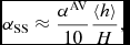 $$\begin{equation}
\alpha _{\rm SS} \approx \frac{\alpha ^{\rm AV}}{10} \frac{\langle h \rangle }{H},
\end{equation}$$
$$\begin{equation}
\alpha _{\rm SS} \approx \frac{\alpha ^{\rm AV}}{10} \frac{\langle h \rangle }{H},
\end{equation}$$
where 〈h〉 is the mean smoothing length on particles in a cylindrical ring at a given radius.
In practice, this means that one must uniformly resolve the scale height in order to obtain a constant αSS in the disc. We have achieved this in simulations to date by choosing the initial surface density profile and the power-law index of the temperature profile (when using a locally isothermal EOS) to ensure that this is the case (Lodato & Pringle Reference Lodato and Pringle2007). Confirmation that the scaling provided by (124) is correct is shown in Figure 4 of Lodato & Price (Reference Lodato and Price2010) and is checked automatically in the Phantom test suite.
In the original implementation (Lodato & Price Reference Lodato and Price2010), we also set the βAV to zero, but this is dangerous if the disc dynamics are complex as there is nothing to prevent particle penetration (see Section 2.2.7). Hence, in the current version of the code, βAV = 2 by default even if disc viscosity is set, but is only applied to approaching particles (c.f. 120). Applying any component of viscosity to only approaching particles can affect the sign of the precession induced in warped discs (Lodato & Pringle Reference Lodato and Pringle2007), but in general retaining the βAV term is safer with no noticeable effect on the overall dissipation due to the second-order dependence of this term on resolution.
Using αAV to set the disc viscosity has two useful consequences. First, it forces one to consider whether or not the scale height, H, is resolved. Second, knowing the value of αAV is helpful, as αAV ≈ 0.1 represents the lower bound below which a physical viscosity is not resolved in SPH (that is, viscosities smaller than this produce disc spreading independent of the value of αAV, see Bate Reference Bate1995; Meru & Bate Reference Meru and Bate2012), while αAV > 1 constrains the timestep (Section 2.3.2).
2.6.2. Disc viscosity using the Navier–Stokes viscosity terms
An alternative approach is to compute viscous terms directly from the Navier–Stokes equation. Details of how the Navier–Stokes terms are represented are given below (Section 2.7), but for disc viscosity a method for determining the kinematic viscosity is needed, which in turn requires specifying the scale height as a function of radius. We use
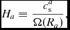 $$\begin{equation}
H_{a} \equiv \frac{c^{a}_{\rm s}}{\Omega (R_{a})},
\end{equation}$$
$$\begin{equation}
H_{a} \equiv \frac{c^{a}_{\rm s}}{\Omega (R_{a})},
\end{equation}$$
where we assume Keplerian rotation 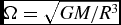 $\Omega = \sqrt{GM/R^{3}}$ and c s is obtained for a given particle from the EOS (which for consistency must be either isothermal or locally isothermal). It is important to note that this restricts the application of this approach only to discs where R can be meaningfully defined, excluding, for example, discs around binary stars.
The shear viscosity is then set using
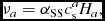 $$\begin{equation}
\nu _{a} = \alpha _{\rm SS} c_{\rm s}^{a} H_{a},
\end{equation}$$
$$\begin{equation}
\nu _{a} = \alpha _{\rm SS} c_{\rm s}^{a} H_{a},
\end{equation}$$
where αSS is a pre-defined/input parameter. The timestep is constrained using C visch 2/ν as described in Section 2.7. The advantage to this approach is that the shear viscosity is set directly and does not depend on the smoothing length. However, as found by Lodato & Price (Reference Lodato and Price2010), it remains necessary to apply some bulk viscosity to capture shocks and prevent particle penetration of the disc midplane, so one should apply the shock viscosity as usual. Using a shock-detection switch (Section 2.2.9) means that this is usually not problematic. This formulation of viscosity was used in Facchini et al. (Reference Facchini, Lodato and Price2013).
2.7. Navier–Stokes viscosity
Physical viscosity is implemented as described in Lodato & Price (Reference Lodato and Price2010). Here, (23) and (24) are replaced by the compressible Navier–Stokes equations, i.e.
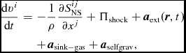 $$\begin{eqnarray}
\frac{{\rm d}v^{i}}{{\rm d}t} &=& -\frac{1}{\rho }\frac{\partial S_{\rm NS}^{ij}}{\partial x^{j}} + \Pi _{\rm shock} + {\bm a}_{\rm ext}({\bm r}, t) \nonumber \\
&& +\, {\bm a}_{\rm sink-gas} + {\bm a}_{\rm selfgrav},
\end{eqnarray}$$
$$\begin{eqnarray}
\frac{{\rm d}v^{i}}{{\rm d}t} &=& -\frac{1}{\rho }\frac{\partial S_{\rm NS}^{ij}}{\partial x^{j}} + \Pi _{\rm shock} + {\bm a}_{\rm ext}({\bm r}, t) \nonumber \\
&& +\, {\bm a}_{\rm sink-gas} + {\bm a}_{\rm selfgrav},
\end{eqnarray}$$
 $$\begin{eqnarray}
\frac{{\rm d}u}{{\rm d}t} = -\frac{P}{\rho } \left(\nabla \cdot {\bm v}\right) + \Lambda _{\rm visc} + \Lambda _{\rm shock} - \frac{\Lambda _{\rm cool}}{\rho },
\end{eqnarray}$$
$$\begin{eqnarray}
\frac{{\rm d}u}{{\rm d}t} = -\frac{P}{\rho } \left(\nabla \cdot {\bm v}\right) + \Lambda _{\rm visc} + \Lambda _{\rm shock} - \frac{\Lambda _{\rm cool}}{\rho },
\end{eqnarray}$$
with the stress tensor given by
 $$\begin{equation}
S_{\rm NS}^{ij} = \left[ P - \left(\zeta - \frac{2}{3}\eta \right) \frac{\partial v^{k}}{\partial x^{k}} \right] \delta ^{ij} - \eta \left( \frac{\partial v^{i}}{\partial x^{j}} + \frac{\partial v^{j}}{\partial x^{i}}\right),
\end{equation}$$
$$\begin{equation}
S_{\rm NS}^{ij} = \left[ P - \left(\zeta - \frac{2}{3}\eta \right) \frac{\partial v^{k}}{\partial x^{k}} \right] \delta ^{ij} - \eta \left( \frac{\partial v^{i}}{\partial x^{j}} + \frac{\partial v^{j}}{\partial x^{i}}\right),
\end{equation}$$
where δij is the Kronecker delta, and ζ and η are the bulk and shear viscosity coefficients, related to the volume and kinematic shear viscosity coefficients by ζv ≡ ζ/ρ and ν ≡ η/ρ.
2.7.1. Physical viscosity using two first derivatives
As there is no clear consensus on the best way to implement physical viscosity in SPH, Phantom currently contains two implementations. The simplest is to use two first derivatives, which is essentially that proposed by Flebbe et al. (Reference Flebbe, Muenzel, Herold, Riffert and Ruder1994), Watkins et al. (Reference Watkins, Bhattal, Francis, Turner and Whitworth1996), and Sijacki & Springel (Reference Sijacki and Springel2006). In this case, (127) is discretised in the standard manner using
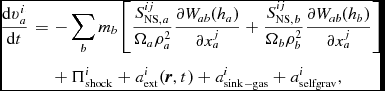 $$\begin{eqnarray}
\frac{{\rm d}v^{i}_{a}}{{\rm d}t} &=& -\sum _{b} m_{b}\left[ \frac{S^{ij}_{{\rm NS}, a}}{\Omega _{a}\rho _{a}^{2}} \frac{\partial W_{ab}(h_{a})}{\partial x^{j}_{a}} + \frac{S^{ij}_{{\rm NS}, b}}{\Omega _{b}\rho _{b}^{2}} \frac{\partial W_{ab}(h_{b})}{\partial x^{j}_{a}}\right] \nonumber \\
&& +\, \Pi ^{i}_{\rm shock} + a^{i}_{\rm ext}({\bm r}, t) + a^{i}_{\rm sink-gas} + a^{i}_{\rm selfgrav},
\end{eqnarray}$$
$$\begin{eqnarray}
\frac{{\rm d}v^{i}_{a}}{{\rm d}t} &=& -\sum _{b} m_{b}\left[ \frac{S^{ij}_{{\rm NS}, a}}{\Omega _{a}\rho _{a}^{2}} \frac{\partial W_{ab}(h_{a})}{\partial x^{j}_{a}} + \frac{S^{ij}_{{\rm NS}, b}}{\Omega _{b}\rho _{b}^{2}} \frac{\partial W_{ab}(h_{b})}{\partial x^{j}_{a}}\right] \nonumber \\
&& +\, \Pi ^{i}_{\rm shock} + a^{i}_{\rm ext}({\bm r}, t) + a^{i}_{\rm sink-gas} + a^{i}_{\rm selfgrav},
\end{eqnarray}$$
where the velocity gradients are computed during the density loop using
 $$\begin{equation}
\frac{\partial v_{a}^{i}}{\partial x_{a}^{j}} = -\frac{1}{\Omega _{a}\rho _{a}} \sum _{b} m_{b} v_{ab}^{i} \nabla _a^{j} W_{ab} (h_{a}).
\end{equation}$$
$$\begin{equation}
\frac{\partial v_{a}^{i}}{\partial x_{a}^{j}} = -\frac{1}{\Omega _{a}\rho _{a}} \sum _{b} m_{b} v_{ab}^{i} \nabla _a^{j} W_{ab} (h_{a}).
\end{equation}$$
Importantly, the differenced SPH operator is used in (131), whereas (130) uses the symmetric gradient operator. The use of conjugate operatorsFootnote 5 is a common requirement in SPH in order to guarantee energy conservation and a positive definite entropy increase from dissipative terms (e.g. Price Reference Price2010; Tricco & Price Reference Tricco and Price2012). Total energy conservation means that
 $$\begin{equation}
\frac{{\rm d}E}{{\rm d}t} = \sum _{a} m_{a} \left( \frac{{\rm d}u_{a}}{{\rm d}t} + v^{i}_{a} \frac{{\rm d}v^{i}_{a}}{{\rm d}t} \right) = 0.
\end{equation}$$
$$\begin{equation}
\frac{{\rm d}E}{{\rm d}t} = \sum _{a} m_{a} \left( \frac{{\rm d}u_{a}}{{\rm d}t} + v^{i}_{a} \frac{{\rm d}v^{i}_{a}}{{\rm d}t} \right) = 0.
\end{equation}$$
This implies a contribution to the thermal energy equation given by
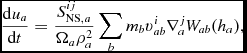 $$\begin{equation}
\frac{{\rm d}u_{a}}{{\rm d}t} = \frac{S_{{\rm NS}, a}^{ij}}{\Omega _{a} \rho _{a}^{2}} \sum _{b} m_{b} v_{ab}^{i} \nabla _a^{j} W_{ab} (h_{a}),
\end{equation}$$
$$\begin{equation}
\frac{{\rm d}u_{a}}{{\rm d}t} = \frac{S_{{\rm NS}, a}^{ij}}{\Omega _{a} \rho _{a}^{2}} \sum _{b} m_{b} v_{ab}^{i} \nabla _a^{j} W_{ab} (h_{a}),
\end{equation}$$
which can be seen to reduce to (24) in the inviscid case (Sij NS = Pδij), but in general is an SPH expression for
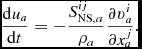 $$\begin{equation}
\frac{{\rm d}u_{a}}{{\rm d}t} = -\frac{S_{{\rm NS}, a}^{ij}}{\rho _{a}} \frac{\partial v_{a}^{i}}{\partial x_{a}^{j}}.
\end{equation}$$
$$\begin{equation}
\frac{{\rm d}u_{a}}{{\rm d}t} = -\frac{S_{{\rm NS}, a}^{ij}}{\rho _{a}} \frac{\partial v_{a}^{i}}{\partial x_{a}^{j}}.
\end{equation}$$
Using Sij NS = S NSji, we have
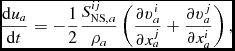 $$\begin{equation}
\frac{{\rm d}u_{a}}{{\rm d}t} = -\frac{1}{2} \frac{S_{{\rm NS}, a}^{ij}}{\rho _{a}} \left( \frac{\partial v_{a}^{i}}{\partial x_{a}^{j}} + \frac{\partial v_{a}^{j}}{\partial x_{a}^{i}} \right),
\end{equation}$$
$$\begin{equation}
\frac{{\rm d}u_{a}}{{\rm d}t} = -\frac{1}{2} \frac{S_{{\rm NS}, a}^{ij}}{\rho _{a}} \left( \frac{\partial v_{a}^{i}}{\partial x_{a}^{j}} + \frac{\partial v_{a}^{j}}{\partial x_{a}^{i}} \right),
\end{equation}$$
which, using (129), gives
 $$\begin{eqnarray}
\Lambda _{\rm visc} = \left(\zeta _{v, a} - \frac{2}{3} \nu _{a} \right) (\nabla \cdot {\bm v})_{a}^{2} + \frac{\nu _{a}}{2} \left( \frac{\partial v_{a}^{i}}{\partial x_{a}^{j}} + \frac{\partial v_{a}^{j}}{\partial x_{a}^{i}} \right)^{2}.
\end{eqnarray}$$
$$\begin{eqnarray}
\Lambda _{\rm visc} = \left(\zeta _{v, a} - \frac{2}{3} \nu _{a} \right) (\nabla \cdot {\bm v})_{a}^{2} + \frac{\nu _{a}}{2} \left( \frac{\partial v_{a}^{i}}{\partial x_{a}^{j}} + \frac{\partial v_{a}^{j}}{\partial x_{a}^{i}} \right)^{2}.
\end{eqnarray}$$
By the square in the last term, we mean the tensor summation ∑j∑iT ijT ij, where Tij ≡ ∂via/∂xja + ∂va j/∂xia. The heating term is therefore positive definite provided that the velocity gradients and divergence are computed using the difference operator (131), both in (136) and when computing the stress tensor (129).
The main disadvantage of the first derivatives approach is that it requires storing the strain tensor for each particle, i.e. six additional quantities when taking account of symmetries.
2.7.2. Physical viscosity with direct second derivatives
The second approach is to use SPH second derivative operators directly. Here we use modified versions of the identities given by Español & Revenga (Reference Español and Revenga2003) (see also Monaghan Reference Monaghan2005; Price Reference Price2012a), namely
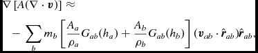 $$\begin{eqnarray}
\hspace*{-38pt}&&\nabla \left[A (\nabla \cdot {\bm v})\right] \approx \nonumber \\
\hspace*{-38pt}&&\quad-\,\sum _{b} m_{b} \left[\frac{A_{a}}{\rho _{a}} G_{ab}(h_{a})+ \frac{A_{b}}{\rho _{b}} G_{ab}(h_{b})\right] ({\bm v}_{ab}\cdot \hat{\bm r}_{ab}) \hat{\bm r}_{ab} ,
\end{eqnarray}$$
$$\begin{eqnarray}
\hspace*{-38pt}&&\nabla \left[A (\nabla \cdot {\bm v})\right] \approx \nonumber \\
\hspace*{-38pt}&&\quad-\,\sum _{b} m_{b} \left[\frac{A_{a}}{\rho _{a}} G_{ab}(h_{a})+ \frac{A_{b}}{\rho _{b}} G_{ab}(h_{b})\right] ({\bm v}_{ab}\cdot \hat{\bm r}_{ab}) \hat{\bm r}_{ab} ,
\end{eqnarray}$$
 $$\begin{eqnarray}
\hspace*{-20pt}\nabla \cdot (C \nabla {\bm v}) \approx -\,\sum _{b} m_{b} \left[\frac{C_{a}}{\rho _{a}} G_{ab}(h_{a}) + \frac{C_{b}}{\rho _{b}} G_{ab}(h_{b})\right]{\bm v}_{ab},
\end{eqnarray}$$
$$\begin{eqnarray}
\hspace*{-20pt}\nabla \cdot (C \nabla {\bm v}) \approx -\,\sum _{b} m_{b} \left[\frac{C_{a}}{\rho _{a}} G_{ab}(h_{a}) + \frac{C_{b}}{\rho _{b}} G_{ab}(h_{b})\right]{\bm v}_{ab},
\end{eqnarray}$$
where G ab ≡ −2F ab/|r ab|, i.e. the scalar part of the kernel gradient divided by the particle separation, which can be thought of as equivalent to defining a new ‘second derivative kernel’ (Brookshaw Reference Brookshaw1985, Reference Brookshaw1994; Price Reference Price2012a; Price & Laibe Reference Price and Laibe2015a).
From the compressible Navier–Stokes equations, (127) with (129), the coefficients in these two terms are
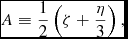 $$\begin{eqnarray}
A \equiv \frac{1}{2} \left(\zeta + \frac{\eta }{3}\right),
\end{eqnarray}$$
$$\begin{eqnarray}
A \equiv \frac{1}{2} \left(\zeta + \frac{\eta }{3}\right),
\end{eqnarray}$$
 $$\begin{eqnarray}
C \equiv \frac{1}{2} \eta ,
\end{eqnarray}$$
$$\begin{eqnarray}
C \equiv \frac{1}{2} \eta ,
\end{eqnarray}$$
so that we can simply use
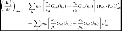 $$\begin{eqnarray}
\left(\frac{{\rm d}v^{i}_{a}}{{\rm d}t}\right)_{\rm visc} &=& \sum_b m_b \left[ \frac{\tau_a}{\rho_a} G_{ab}(h_a) + \frac{\tau_b}{\rho_b} G_{ab}(h_b) \right] ({\bm v}_{ab}\cdot \hat{\bm r}_{ab})\hat{r}^i_{ab} \nonumber\\
&&+\, \sum_b m_b \left[ \frac{\kappa_a}{\rho_a} G_{ab}(h_a) + \frac{\kappa_b}{\rho_b} G_{ab}(h_b)\right] v_{ab}^i
\end{eqnarray}$$
$$\begin{eqnarray}
\left(\frac{{\rm d}v^{i}_{a}}{{\rm d}t}\right)_{\rm visc} &=& \sum_b m_b \left[ \frac{\tau_a}{\rho_a} G_{ab}(h_a) + \frac{\tau_b}{\rho_b} G_{ab}(h_b) \right] ({\bm v}_{ab}\cdot \hat{\bm r}_{ab})\hat{r}^i_{ab} \nonumber\\
&&+\, \sum_b m_b \left[ \frac{\kappa_a}{\rho_a} G_{ab}(h_a) + \frac{\kappa_b}{\rho_b} G_{ab}(h_b)\right] v_{ab}^i
\end{eqnarray}$$
where
 $$\begin{eqnarray}
\tau = \frac{5}{2} A,
\end{eqnarray}$$
$$\begin{eqnarray}
\tau = \frac{5}{2} A,
\end{eqnarray}$$
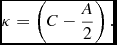 $$\begin{eqnarray}
\kappa = \left(C - \frac{A}{2}\right).
\end{eqnarray}$$
$$\begin{eqnarray}
\kappa = \left(C - \frac{A}{2}\right).
\end{eqnarray}$$
The corresponding heating terms in the thermal energy equation are given by
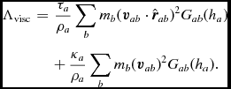 $$\begin{eqnarray}
\Lambda _{\rm visc} &=& \frac{\tau _{a}}{\rho _{a}} \sum _{b} m_{b} ({\bm v}_{ab}\cdot \hat{\bm r}_{ab})^{2} G_{ab}(h_{a}) \nonumber \\
&& +\, \frac{\kappa _{a}}{\rho _{a}} \sum _{b} m_{b} ({\bm v}_{ab})^{2} G_{ab}(h_{a}).
\end{eqnarray}$$
$$\begin{eqnarray}
\Lambda _{\rm visc} &=& \frac{\tau _{a}}{\rho _{a}} \sum _{b} m_{b} ({\bm v}_{ab}\cdot \hat{\bm r}_{ab})^{2} G_{ab}(h_{a}) \nonumber \\
&& +\, \frac{\kappa _{a}}{\rho _{a}} \sum _{b} m_{b} ({\bm v}_{ab})^{2} G_{ab}(h_{a}).
\end{eqnarray}$$
This is the default formulation of Navier–Stokes viscosity in the code since it does not require additional storage. In practice, we have found little difference between the two formulations of physical viscosity, but this would benefit from a detailed study. In general one might expect the two first derivatives formulation to offer a less noisy estimate at the cost of additional storage. However, direct second derivatives are the method used in ‘Smoothed Dissipative Particle Dynamics’ (Español & Revenga Reference Español and Revenga2003).
2.7.3. Timestep constraint
Both approaches to physical viscosity use explicit timestepping, and therefore imply a constraint on the timestep given by
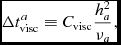 $$\begin{equation}
\Delta t^{a}_{\rm visc} \equiv C_{\rm visc} \frac{h_{a}^{2}}{\nu _{a}},
\end{equation}$$
$$\begin{equation}
\Delta t^{a}_{\rm visc} \equiv C_{\rm visc} \frac{h_{a}^{2}}{\nu _{a}},
\end{equation}$$
where C visc = 0.25 by default (Brookshaw Reference Brookshaw1994). When physical viscosity is turned on, this constraint is included with other timestep constraints according to (77).
2.7.4. Physical viscosity and the tensile instability
Caution is required in the use of physical viscosity at high Mach number, since negative stress can lead to the tensile instability (Morris Reference Morris1996b; Monaghan Reference Monaghan2000; Gray, Monaghan, & Swift Reference Gray, Monaghan and Swift2001). For subsonic applications, this is usually not a problem since the strain tensor and velocity divergence are small compared to the pressure. In the current code, we simply emit a warning if physical viscosity leads to negative stresses during the calculation, but this would benefit from a detailed study.
2.7.5. Physical viscosity and angular momentum conservation
Neither method for physical viscosity exactly conserves angular momentum because the force is no longer directed along the line of sight joining the particles. However, the error is usually small (see discussion in Bonet & Lok Reference Bonet and Lok1999, Section 5 of Price & Monaghan Reference Price and Monaghan2004b or Hu & Adams Reference Hu and Adams2006). Recently, Müller, Fedosov, & Gompper (Reference Müller, Fedosov and Gompper2015) have proposed an algorithm for physical viscosity in SPH that explicitly conserves angular momentum by tracking particle spin, which may be worth investigating.
2.8. Sink particles
Sink particles were introduced into SPH by Bate, Bonnell, & Price (Reference Bate, Bonnell and Price1995) in order to follow star formation simulations beyond the point of fragmentation. In Phantom, these are treated separately to the SPH particles, and interact with other particles, including other sink particles, only via gravity. The differences with other point-mass particles implemented in the code (e.g. dust, stars, and dark matter) are that (i) the gravitational interaction is computed using a direct N 2 summation which is not softened by default (i.e., the N-body algorithm is collisional); (ii) they are allowed to accrete gas; and (iii) they store the accreted angular momentum and other extended properties, such as the accreted mass. Sink particles are evolved in time using the RESPA algorithm (Section 2.3.3), which is second-order accurate, symplectic, and allows sink particles to evolve on shorter timesteps compared to SPH particles.
2.8.1. Sink particle accelerations
The equations of motion for a given sink particle, i, are
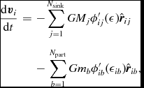 $$\begin{eqnarray}
\frac{{\rm d}{\bm v}_{i}}{{\rm d}t} &= & -\sum ^{N_{\rm sink}}_{j=1} G M_{j} \phi ^{\prime }_{ij} (\epsilon ) \hat{\bm r}_{ij} \nonumber \\
&& -\, \sum ^{N_{\rm part}}_{b=1} G m_{b} \phi ^{\prime }_{ib} (\epsilon _{ib}) \hat{\bm r}_{ib},
\end{eqnarray}$$
$$\begin{eqnarray}
\frac{{\rm d}{\bm v}_{i}}{{\rm d}t} &= & -\sum ^{N_{\rm sink}}_{j=1} G M_{j} \phi ^{\prime }_{ij} (\epsilon ) \hat{\bm r}_{ij} \nonumber \\
&& -\, \sum ^{N_{\rm part}}_{b=1} G m_{b} \phi ^{\prime }_{ib} (\epsilon _{ib}) \hat{\bm r}_{ib},
\end{eqnarray}$$
where ϕ′ab is the softening kernel (Section 2.12.2), N part is the total number of gas particles, and N sink is the total number of sink particles. The sink–gas softening length, εib, is defined as the maximum of the (fixed) softening length defined for the sink particles, ε, and the softening length of the gas particle, εb. That is, εib ≡ max(ε, εb). SPH particles receive a corresponding acceleration
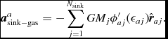 $$\begin{equation}
{\bm a}^{a}_{\rm sink-gas} = -\sum ^{N_{\rm sink}}_{j=1} G M_{j} \phi ^{\prime }_{aj} (\epsilon _{aj}) \hat{\bm r}_{aj}.
\end{equation}$$
$$\begin{equation}
{\bm a}^{a}_{\rm sink-gas} = -\sum ^{N_{\rm sink}}_{j=1} G M_{j} \phi ^{\prime }_{aj} (\epsilon _{aj}) \hat{\bm r}_{aj}.
\end{equation}$$
Softening of sink–gas interactions is not applied if the softening length for sink particles is set to zero, in which case the sink–gas accelerations reduce simply to
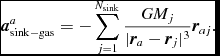 $$\begin{equation}
{\bm a}^{a}_{\rm sink-gas} = -\sum ^{N_{\rm sink}}_{j=1} \frac{G M_{j}}{\vert {\bm r}_{a} - {\bm r}_{j}\vert ^{3}} {\bm r}_{aj}.
\end{equation}$$
$$\begin{equation}
{\bm a}^{a}_{\rm sink-gas} = -\sum ^{N_{\rm sink}}_{j=1} \frac{G M_{j}}{\vert {\bm r}_{a} - {\bm r}_{j}\vert ^{3}} {\bm r}_{aj}.
\end{equation}$$
This is the default behaviour when sink particles are used in the code. Softening of sink–gas interactions is useful to model a point-mass particle that does not accrete gas (e.g. by setting the accretion radius to zero). For example, we used a softened sink particle to simulate the core of the red giant in Iaconi et al. (Reference Iaconi, Reichardt, Staff, De Marco, Passy, Price, Wurster and Herwig2017). The sink–sink interaction is unsoftened by default (ε = 0), giving the usual
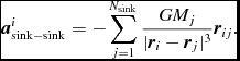 $$\begin{equation}
{\bm a}^{i}_{\rm sink-sink} = -\sum ^{N_{\rm sink}}_{j=1} \frac{G M_{j}}{ \vert {\bm r}_{i} - {\bm r}_{j}\vert ^{3}} {\bm r}_{ij}.
\end{equation}$$
$$\begin{equation}
{\bm a}^{i}_{\rm sink-sink} = -\sum ^{N_{\rm sink}}_{j=1} \frac{G M_{j}}{ \vert {\bm r}_{i} - {\bm r}_{j}\vert ^{3}} {\bm r}_{ij}.
\end{equation}$$
Caution is required when integrating tight binary or multiple systems when ε = 0 to ensure that the timestep conditions (Section 2.3.2) are strict enough.
2.8.2. Accretion onto sink particles
Accretion of gas particles onto a sink particle occurs when a gas particle passes a series of accretion checks within the accretion radius r acc of a sink particle (set in the initial conditions or when the sink particle is created, see Section 2.8.4). First, a gas particle is indiscriminately accreted without undergoing any additional checks if it falls within f accr acc, where 0 ⩽ f acc ⩽ 1 (default f acc = 0.8). In the boundary region f accr acc < r < r acc, a gas particle undergoes accretion if
1. $\vert {\bm L}_{ai} \vert < \vert {\bm L}_{\rm acc} \vert$, that is, its specific angular momentum is less than that of a Keplerian orbit at r acc,
2.
$e = \frac{v_{ai}^2}{2} - \frac{GM_i}{r_{ai}} < 0$, i.e., it is gravitationally bound to the sink particle, and3. e for this gas–sink pair is smaller than e with any other sink particle, that is, out of all sink particles, the gas particle is most bound to this one.

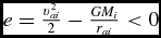
In the above conditions,  ${\bm L}_{ai}$ is the relative specific angular momentum of the gas–sink pair, a − i, defined by
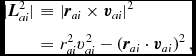 $$\begin{eqnarray}
\vert {\bm L}_{ai}^2\vert & \equiv& \vert {\bm r}_{ai} \times {\bm v}_{ai}\vert ^2 \nonumber \\
& = &r_{ai}^2v_{ai}^2 - \left({\bm r}_{ai}\cdot {\bm v}_{ai}\right)^2,
\end{eqnarray}$$
$$\begin{eqnarray}
\vert {\bm L}_{ai}^2\vert & \equiv& \vert {\bm r}_{ai} \times {\bm v}_{ai}\vert ^2 \nonumber \\
& = &r_{ai}^2v_{ai}^2 - \left({\bm r}_{ai}\cdot {\bm v}_{ai}\right)^2,
\end{eqnarray}$$
while  $\vert {\bm L}_{\rm acc} \vert = r_{\rm acc}^2 \Omega _{\rm acc}$ is the angular momentum at r acc, where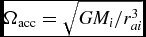 $\Omega _{\rm acc} = \sqrt{GM_i / r_{ai}^{3}}$ is the Keplerian angular speed at r acc, v ai, and r ai are the relative velocity and position, respectively, and M i is the mass of the sink particle.
When a particle, a, passes the accretion checks, then the mass, position, velocity, acceleration, and spin angular momentum of the sink particle are updated according to
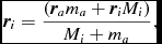 $$\begin{eqnarray}
{\bm r}_{i} = \frac{({\bm r}_{a} m_{a} + {\bm r}_{i} M_{i})}{M_{i} + m_{a}},
\end{eqnarray}$$
$$\begin{eqnarray}
{\bm r}_{i} = \frac{({\bm r}_{a} m_{a} + {\bm r}_{i} M_{i})}{M_{i} + m_{a}},
\end{eqnarray}$$
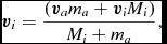 $$\begin{eqnarray}
{\bm v}_{i} = \frac{({\bm v}_{a} m_{a} + {\bm v}_{i} M_{i})}{M_{i} + m_{a}},
\end{eqnarray}$$
$$\begin{eqnarray}
{\bm v}_{i} = \frac{({\bm v}_{a} m_{a} + {\bm v}_{i} M_{i})}{M_{i} + m_{a}},
\end{eqnarray}$$
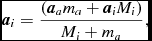 $$\begin{eqnarray}
{\bm a}_{i} = \frac{({\bm a}_{a} m_{a} + {\bm a}_{i} M_{i})}{M_{i} + m_{a}},
\end{eqnarray}$$
$$\begin{eqnarray}
{\bm a}_{i} = \frac{({\bm a}_{a} m_{a} + {\bm a}_{i} M_{i})}{M_{i} + m_{a}},
\end{eqnarray}$$
 $$\begin{eqnarray}
{\bm S}_{i} = {\bm S}_{i} +\frac{m_{a} M_{i}}{M_{i} + m_{a}} \left[ \left({\bm r}_{a} - {\bm r}_{i}\right) \times \left({\bm v}_{a} - {\bm v}_{i}\right)\right],
\end{eqnarray}$$
$$\begin{eqnarray}
{\bm S}_{i} = {\bm S}_{i} +\frac{m_{a} M_{i}}{M_{i} + m_{a}} \left[ \left({\bm r}_{a} - {\bm r}_{i}\right) \times \left({\bm v}_{a} - {\bm v}_{i}\right)\right],
\end{eqnarray}$$
 $$\begin{eqnarray}
M_{i} = M_{i} + m_{a}.
\end{eqnarray}$$
$$\begin{eqnarray}
M_{i} = M_{i} + m_{a}.
\end{eqnarray}$$
This ensures that mass, linear momentum, and angular momentum (but not energy) are conserved by the accretion process. The accreted mass as well as the total mass for each sink particle is stored to avoid problems with round-off error in the case where the particle masses are much smaller than the sink mass. Accreted particles are tagged by setting their smoothing lengths negative. Those particles with h ⩽ 0 are subsequently excluded when the kd-tree is built.
2.8.3. Sink particle boundary conditions
No special sink particle boundary conditions are implemented in Phantom at present. More advanced boundary conditions to regularise the density, pressure, and angular momentum near a sink have been proposed by Bate et al. (Reference Bate, Bonnell and Price1995) and used in Bate & Bonnell (Reference Bate and Bonnell1997), and proposed again more recently by Hubber, Walch, & Whitworth (Reference Hubber, Walch and Whitworth2013b). While these conditions help to regularise the flow near the sink particle, they can also cause problems—particularly the angular momentum boundary condition if the disc near the sink particle has complicated structure such as spiral density waves (Bate 2014, private communication). Often it is more cost effective to simply reduce the accretion radius of the sink. This may change in future code versions.
2.8.4. Dynamic sink particle creation
As described in Bate et al. (Reference Bate, Bonnell and Price1995), it is also possible to create sink particles on-the-fly provided certain physical conditions are met and self-gravity is turned on (Section 2.12). The primary conditions required for sink particle formation are that the density of a given particle exceeds some threshold physical density somewhere in the domain, and that this density peak occurs more than a critical distance r crit from an existing sink. Once these conditions are met on a particular particle, a, the creation of a new sink particle occurs by passing the following conditions (Bate et al. Reference Bate, Bonnell and Price1995):
1. The particle is a gas particle.
2.
$\nabla \cdot {\bm v}_{a} \le 0$, that is, gas surrounding the particle is at rest or collapsing.3. h a < r acc/2, i.e., the smoothing length of the particle is less than half of the accretion radius.
4. All neighbours within r acc are currently active.
5. The ratio of thermal to gravitational energy of particles within r acc, αJ, satisfies αJ ⩽ 1/2.
6. αJ + βrot ⩽ 1, where βrot = |e rot|/|e grav| is the ratio of rotational energy to the magnitude of the gravitational energy for particles within r acc.
7. e tot < 0, that is, the total energy of particles within r acc is negative (i.e. the clump is gravitationally bound).
8. The particle is at a local potential minimum, i.e. Φ is less than Φ computed on all other particles within r acc (Federrath et al. Reference Federrath, Banerjee, Clark and Klessen2010b).

A new sink particle is created at the position of particle a if these checks are passed, and immediately the particles within r acc are accreted by calling the routine described in Section 2.8.2. The checks above are the same as those in Bate et al. (Reference Bate, Bonnell and Price1995), with the additional check from Federrath et al. (Reference Federrath, Banerjee, Clark and Klessen2010b) to ensure that sink particles are only created in a local minimum of the gravitational potential.
The various energies used to evaluate the criteria above are computed according to
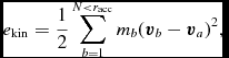 $$\begin{eqnarray}
\hspace*{-26.2pt}e_{\rm kin} = \frac{1}{2} \sum ^{N<r_{\rm acc}}_{b=1} m_{b} ({\bm v}_{b} - {\bm v}_{a})^{2},\hspace*{26.2pt}
\end{eqnarray}$$
$$\begin{eqnarray}
\hspace*{-26.2pt}e_{\rm kin} = \frac{1}{2} \sum ^{N<r_{\rm acc}}_{b=1} m_{b} ({\bm v}_{b} - {\bm v}_{a})^{2},\hspace*{26.2pt}
\end{eqnarray}$$
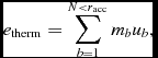 $$\begin{eqnarray}
\hspace*{-49.14pt}e_{\rm therm} = \sum ^{N<r_{\rm acc}}_{b=1} m_{b} u_{b},\hspace*{49.14pt}
\end{eqnarray}$$
$$\begin{eqnarray}
\hspace*{-49.14pt}e_{\rm therm} = \sum ^{N<r_{\rm acc}}_{b=1} m_{b} u_{b},\hspace*{49.14pt}
\end{eqnarray}$$
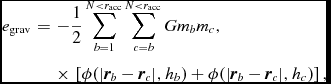 $$\begin{eqnarray}
e_{\rm grav} = -\frac{1}{2}\sum ^{N<r_{\rm acc}}_{b=1}\sum ^{N<r_{\rm acc}}_{c=b} G m_{b} m_{c} , \nonumber \\
&& \times\, \left[\phi (\vert {\bm r}_{b} - {\bm r}_{c}\vert , h_b) + \phi (\vert {\bm r}_{b} - {\bm r}_{c}\vert , h_c)\right],
\end{eqnarray}$$
$$\begin{eqnarray}
e_{\rm grav} = -\frac{1}{2}\sum ^{N<r_{\rm acc}}_{b=1}\sum ^{N<r_{\rm acc}}_{c=b} G m_{b} m_{c} , \nonumber \\
&& \times\, \left[\phi (\vert {\bm r}_{b} - {\bm r}_{c}\vert , h_b) + \phi (\vert {\bm r}_{b} - {\bm r}_{c}\vert , h_c)\right],
\end{eqnarray}$$
 $$\begin{eqnarray}
e_{\rm tot} = e_{\rm kin} + e_{\rm therm} + e_{\rm grav},
\end{eqnarray}$$
$$\begin{eqnarray}
e_{\rm tot} = e_{\rm kin} + e_{\rm therm} + e_{\rm grav},
\end{eqnarray}$$
 $$\begin{eqnarray}
e_{\rm rot} \equiv \sqrt{e^{2}_{{\rm rot}, x} + e^{2}_{{\rm rot}, y} + e^{2}_{{\rm rot}, z}},
\end{eqnarray}$$
$$\begin{eqnarray}
e_{\rm rot} \equiv \sqrt{e^{2}_{{\rm rot}, x} + e^{2}_{{\rm rot}, y} + e^{2}_{{\rm rot}, z}},
\end{eqnarray}$$
 $$\begin{eqnarray}
e_{{\rm rot}, x} \equiv \frac{1}{2} \sum ^{N<r_{\rm acc}}_{b=1} m_{b} \frac{L^{2}_{{ab},x}}{\sqrt{(y_{a} - y_{b})^{2} + (z_{a} - z_{b})^{2}}},
\end{eqnarray}$$
$$\begin{eqnarray}
e_{{\rm rot}, x} \equiv \frac{1}{2} \sum ^{N<r_{\rm acc}}_{b=1} m_{b} \frac{L^{2}_{{ab},x}}{\sqrt{(y_{a} - y_{b})^{2} + (z_{a} - z_{b})^{2}}},
\end{eqnarray}$$
 $$\begin{eqnarray}
e_{{\rm rot}, y} \equiv \frac{1}{2} \sum ^{N<r_{\rm acc}}_{b=1} m_{b} \frac{L^{2}_{{ab},y}}{\sqrt{(x_{a} - x_{b})^{2} + (z_{a} - z_{b})^{2}}},
\end{eqnarray}$$
$$\begin{eqnarray}
e_{{\rm rot}, y} \equiv \frac{1}{2} \sum ^{N<r_{\rm acc}}_{b=1} m_{b} \frac{L^{2}_{{ab},y}}{\sqrt{(x_{a} - x_{b})^{2} + (z_{a} - z_{b})^{2}}},
\end{eqnarray}$$
 $$\begin{eqnarray}
e_{{\rm rot}, z} \equiv \frac{1}{2} \sum ^{N<r_{\rm acc}}_{b=1} m_{b} \frac{L^{2}_{{ab},z}}{\sqrt{(x_{a} - x_{b})^{2} + (y_{a} - y_{b})^{2}}},
\end{eqnarray}$$
$$\begin{eqnarray}
e_{{\rm rot}, z} \equiv \frac{1}{2} \sum ^{N<r_{\rm acc}}_{b=1} m_{b} \frac{L^{2}_{{ab},z}}{\sqrt{(x_{a} - x_{b})^{2} + (y_{a} - y_{b})^{2}}},
\end{eqnarray}$$
where  ${\bm L}_{ab} \equiv ({\bm r}_{a} - {\bm r}_{b}) \times ({\bm v}_{a} - {\bm v}_{b})$ is the specific angular momentum between a pair of particles, and ϕ is the gravitational softening kernel (defined in Section 2.12), which has units of inverse length. Adding the contribution from all pairs, b − c, within the clump is required to obtain the total potential of the clump.
2.8.5. Sink particle timesteps
Sink particles are integrated together with a global, but adaptive, timestep, following the inner loop of the RESPA algorithm given in (80)–(83) corresponding to a second-order Leapfrog integration. The timestep is controlled by the minimum of the sink–gas timestep, (75), and a sink–sink timestep (Dehnen & Read Reference Dehnen and Read2011)
 $$\begin{equation}
\Delta t_{\rm sink-sink} \equiv \min _{i} \left( C_{\rm force} \eta _\Phi \sqrt{\frac{\vert \Phi ^{\rm sink-sink}_{i}\vert }{\vert \nabla \Phi ^{\rm sink-sink}_i \vert ^{2}}} \right),
\end{equation}$$
$$\begin{equation}
\Delta t_{\rm sink-sink} \equiv \min _{i} \left( C_{\rm force} \eta _\Phi \sqrt{\frac{\vert \Phi ^{\rm sink-sink}_{i}\vert }{\vert \nabla \Phi ^{\rm sink-sink}_i \vert ^{2}}} \right),
\end{equation}$$
where the potential and gradient include other sink particles, plus any external potentials applied to sink particles except the sink–gas potential. We set  $\eta _\Phi = 0.05$ by default, resulting in ~300–500 steps per orbit for a binary orbit with the default C force = 0.25 (see Section 5.5.1).
More accurate integrators such as the fourth-order Hermite scheme (Makino & Aarseth Reference Makino and Aarseth1992) or the fourth-order symplectic schemes proposed by Omelyan, Mryglod, & Folk (Reference Omelyan, Mryglod and Folk2002) or Chin & Chen (Reference Chin and Chen2005) are not yet implemented in Phantom, but it would be a worthwhile effort to incorporate one of these in a future code version. See Hubber et al. (Reference Hubber, Allison, Smith and Goodwin2013a) for a recent implementation of a fourth-order Hermite scheme for sink particles in SPH.
2.9. Stellar physics
A tabulated EOS can be used to take account of the departure from an ideal gas, for example, due to changes in ionisation or molecular dissociation and recombination. This tabulated EOS in Phantom is adapted from the logP gas − T EOS tables provided with the open source package Modules for Experiments in Stellar Astrophysics mesa (Paxton et al. Reference Paxton, Bildsten, Dotter, Herwig, Lesaffre and Timmes2011). Details of the data, originally compiled from blends of equations of state from Saumon, Chabrier, & van Horn (Reference Saumon, Chabrier and van Horn1995) (SCVH), Timmes & Swesty (Reference Timmes and Swesty2000), Rogers & Nayfonov (Reference Rogers and Nayfonov2002, also the 2005 update), Potekhin & Chabrier (Reference Potekhin and Chabrier2010) and for an ideal gas, are outlined by Paxton et al. (Reference Paxton, Bildsten, Dotter, Herwig, Lesaffre and Timmes2011).
In our implementation (adapted from original routines for the Music code; Goffrey et al. Reference Goffrey2017), we compute the pressure and other required EOS variables for a particular composition by interpolation between sets of tables for different hydrogen abundance X = 0.0, 0.2, 0.4, 0.6, 0.8 and metallicity Z = 0.0, 0.02, 0.04. Pressure is calculated with bicubic interpolation, and Γ1 ≡ ∂lnP/∂lnρ|s with bilinear interpolation, in logu and logV ≡ logρ − 0.7logu + 20. The tables are currently valid in the ranges 10.5 ⩽ logu ⩽ 17.5 and 0.0 ⩽ logV ⩽ 14.0. Values requested outside the tables are currently computed by linear extrapolation. This triggers a warning to the user.
We have not tested the thermodynamic consistency of our interpolation scheme from the tables (Timmes & Arnett Reference Timmes and Arnett1999).
2.10. Magnetohydrodynamics
Phantom implements the smoothed particle magnetohydrodynamics (SPMHD) algorithm described in Price (Reference Price2012a) and Tricco & Price (Reference Tricco and Price2012, Reference Tricco and Price2013), based on the original work by Phillips & Monaghan (Reference Phillips and Monaghan1985) and Price & Monaghan (Reference Price and Monaghan2004a, Reference Price and Monaghan2004b, Reference Price and Monaghan2005). Phantom was previously used to test a vector potential formulation (Price Reference Price2010), but this algorithm has been subsequently removed from the code due to its poor performance (see Price Reference Price2010).
The important difference between Phantom and the gadget implementation of SPMHD (Dolag & Stasyszyn Reference Dolag and Stasyszyn2009; Bürzle et al. Reference Bürzle, Clark, Stasyszyn, Greif, Dolag, Klessen and Nielaba2011a, Reference Bürzle, Clark, Stasyszyn, Dolag and Klessen2011b), which also implements the core algorithms from Price & Monaghan (Reference Price and Monaghan2004a, Reference Price and Monaghan2004b, Reference Price and Monaghan2005), is our use of the divergence-cleaning algorithm from Tricco & Price (Reference Tricco and Price2012, Reference Tricco and Price2013) and Tricco, Price, & Bate (Reference Tricco, Price and Bate2016a). This is vital for preserving the divergence-free (no monopoles) condition on the magnetic field.
For recent applications of Phantom to MHD problems, see e.g. Tricco et al. (Reference Tricco, Price and Federrath2016b), Dobbs et al. (Reference Dobbs, Price, Pettitt, Bate and Tricco2016), Bonnerot et al. (Reference Bonnerot, Price, Lodato and Rossi2017), Forgan, Price, & Bonnell (Reference Forgan, Price and Bonnell2017), and Wurster et al. (Reference Wurster, Price and Bate2016, Reference Wurster, Price and Bate2017).
2.10.1. Equations of magnetohydrodynamics
Phantom solves the equations of MHD in the form
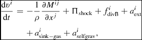 $$\begin{eqnarray}
\frac{{\rm d}v^{i}}{{\rm d}t} &=& -\frac{1}{\rho }\frac{\partial M^{ij}}{\partial x^{j}} + \Pi _{\rm shock} + f^{i}_{\rm divB} + a^{i}_{\rm ext} \nonumber \\
&& +\, a^{i}_{\rm sink-gas} + a^{i}_{\rm selfgrav},
\end{eqnarray}$$
$$\begin{eqnarray}
\frac{{\rm d}v^{i}}{{\rm d}t} &=& -\frac{1}{\rho }\frac{\partial M^{ij}}{\partial x^{j}} + \Pi _{\rm shock} + f^{i}_{\rm divB} + a^{i}_{\rm ext} \nonumber \\
&& +\, a^{i}_{\rm sink-gas} + a^{i}_{\rm selfgrav},
\end{eqnarray}$$
 $$\begin{eqnarray}
\frac{{\rm d}u}{{\rm d}t} = -\frac{P}{\rho } \left(\nabla \cdot {\bm v}\right) + \Lambda _{\rm shock} - \frac{\Lambda _{\rm cool}}{\rho },
\end{eqnarray}$$
$$\begin{eqnarray}
\frac{{\rm d}u}{{\rm d}t} = -\frac{P}{\rho } \left(\nabla \cdot {\bm v}\right) + \Lambda _{\rm shock} - \frac{\Lambda _{\rm cool}}{\rho },
\end{eqnarray}$$
 $$\begin{eqnarray}
\frac{{\rm d}}{{\rm d}t} \left(\frac{\bm B}{\rho } \right) = \frac{1}{\rho } \left[ \left({\bm B}\cdot \nabla \right){\bm v} - \nabla \psi + \mathcal {\bm D}_{\rm diss} \right],
\end{eqnarray}$$
$$\begin{eqnarray}
\frac{{\rm d}}{{\rm d}t} \left(\frac{\bm B}{\rho } \right) = \frac{1}{\rho } \left[ \left({\bm B}\cdot \nabla \right){\bm v} - \nabla \psi + \mathcal {\bm D}_{\rm diss} \right],
\end{eqnarray}$$
 $$\begin{eqnarray}
\frac{{\rm d}}{{\rm d}t} \left( \frac{\psi }{c_{\rm h}} \right) = -c_{\rm h} \left(\nabla \cdot {\bm B}\right) - \frac{1}{2} \frac{\psi }{c_{\rm h}} \left(\nabla \cdot {\bm v}\right) - \frac{\psi }{c_{\rm h}\tau _{\rm c}},
\end{eqnarray}$$
$$\begin{eqnarray}
\frac{{\rm d}}{{\rm d}t} \left( \frac{\psi }{c_{\rm h}} \right) = -c_{\rm h} \left(\nabla \cdot {\bm B}\right) - \frac{1}{2} \frac{\psi }{c_{\rm h}} \left(\nabla \cdot {\bm v}\right) - \frac{\psi }{c_{\rm h}\tau _{\rm c}},
\end{eqnarray}$$
where  ${\bm B}$ is the magnetic field, ψ is a scalar used to control the divergence error in the magnetic field (see Section 2.10.8), and $\mathcal {D}_{\rm diss}$ represents magnetic dissipation terms (Sections 2.10.5 and 2.11). The Maxwell stress tensor, M ij, is given by
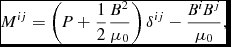 $$\begin{equation}
M^{ij} = \left( P + \frac{1}{2} \frac{B^{2}}{\mu _{0}} \right) \delta ^{ij} - \frac{B^{i} B^{j}}{\mu _{0}},
\end{equation}$$
$$\begin{equation}
M^{ij} = \left( P + \frac{1}{2} \frac{B^{2}}{\mu _{0}} \right) \delta ^{ij} - \frac{B^{i} B^{j}}{\mu _{0}},
\end{equation}$$
where δij is the Kronecker delta and μ0 is the permeability of free space. A source term related to the numerically induced divergence of the magnetic field, given by
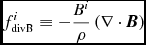 $$\begin{equation}
f^{i}_{\rm divB} \equiv - \frac{B^{i}}{\rho }\left(\nabla \cdot {\bm B}\right)
\end{equation}$$
$$\begin{equation}
f^{i}_{\rm divB} \equiv - \frac{B^{i}}{\rho }\left(\nabla \cdot {\bm B}\right)
\end{equation}$$
is necessary to prevent the tensile instability in SPMHD (Phillips & Monaghan Reference Phillips and Monaghan1985; Monaghan Reference Monaghan2000; Børve, Omang, & Trulsen Reference Børve, Omang and Trulsen2001; Price Reference Price2012a). With this source term, the equation set for ideal MHD in the absence of the divergence cleaning field, ψ, is formally the same as in the Powell et al. (Reference Powell, Roe, Linde, Gombosi and de Zeeuw1999) eight-wave scheme (Price Reference Price2012a), meaning that the divergence errors in the magnetic field are advected by the flow, but not dissipated, unless cleaning is used.
2.10.2. Discrete equations
The discrete version of (165) follows the same procedure as for physical viscosity (Section 2.7), i.e.
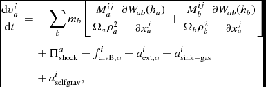 $$\begin{eqnarray}
\frac{{\rm d}v^{i}_{a}}{{\rm d}t} &=& -\sum _{b} m_{b}\left[ \frac{M^{ij}_{a}}{\Omega _{a}\rho _{a}^{2}} \frac{\partial W_{ab}(h_{a})}{\partial x^{j}_{a}} + \frac{M^{ij}_{b}}{\Omega _{b}\rho _{b}^{2}} \frac{\partial W_{ab}(h_{b})}{\partial x^{j}_{a}}\right] \nonumber \\
&& + \,\Pi _{\rm shock}^{a} + f^{i}_{{\rm divB}, a} + a^{i}_{{\rm ext}, a} + a^i_{\rm sink-gas} \nonumber \\
&& +\, a^i_{\rm selfgrav},
\end{eqnarray}$$
$$\begin{eqnarray}
\frac{{\rm d}v^{i}_{a}}{{\rm d}t} &=& -\sum _{b} m_{b}\left[ \frac{M^{ij}_{a}}{\Omega _{a}\rho _{a}^{2}} \frac{\partial W_{ab}(h_{a})}{\partial x^{j}_{a}} + \frac{M^{ij}_{b}}{\Omega _{b}\rho _{b}^{2}} \frac{\partial W_{ab}(h_{b})}{\partial x^{j}_{a}}\right] \nonumber \\
&& + \,\Pi _{\rm shock}^{a} + f^{i}_{{\rm divB}, a} + a^{i}_{{\rm ext}, a} + a^i_{\rm sink-gas} \nonumber \\
&& +\, a^i_{\rm selfgrav},
\end{eqnarray}$$
where Mija is defined according to (169), f divB is a correction term for stability (discussed below), and accelerations due to external forces are as described in Section 2.4.
Equations (167) and (168) are discretised according to (Price & Monaghan Reference Price and Monaghan2005; Tricco & Price Reference Tricco and Price2012; Tricco et al. Reference Tricco, Price and Bate2016a)
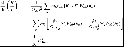 $$\begin{eqnarray}
\frac{{\rm d}}{{\rm d}t} \left( \frac{{\bm B}}{\rho } \right)_a &=& -\frac{1}{\Omega _{a} \rho _{a}^2} \sum _{b} m_{b} {\bm v}_{ab} \left[ {\bm B}_{a} \cdot \nabla _a W_{ab}(h_{a})\right] \nonumber \\
&& -\, \sum _{b} m_{b} \left[ \frac{\psi _{a}}{\Omega _{a}\rho _{a}^{2}} \nabla _a W_{ab}(h_{a})+ \frac{\psi _{b}}{\Omega _{b}\rho _{b}^{2}} \nabla _a W_{ab}(h_{b})\right] \nonumber \\
&& +\, \frac{1}{\rho _a} \mathcal {D}^{a}_{\rm diss},
\end{eqnarray}$$
$$\begin{eqnarray}
\frac{{\rm d}}{{\rm d}t} \left( \frac{{\bm B}}{\rho } \right)_a &=& -\frac{1}{\Omega _{a} \rho _{a}^2} \sum _{b} m_{b} {\bm v}_{ab} \left[ {\bm B}_{a} \cdot \nabla _a W_{ab}(h_{a})\right] \nonumber \\
&& -\, \sum _{b} m_{b} \left[ \frac{\psi _{a}}{\Omega _{a}\rho _{a}^{2}} \nabla _a W_{ab}(h_{a})+ \frac{\psi _{b}}{\Omega _{b}\rho _{b}^{2}} \nabla _a W_{ab}(h_{b})\right] \nonumber \\
&& +\, \frac{1}{\rho _a} \mathcal {D}^{a}_{\rm diss},
\end{eqnarray}$$
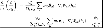 $$\begin{eqnarray}
\frac{{\rm d}}{{\rm d}t} \left(\frac{\psi }{c_{\rm h}} \right)_a &=& \frac{c_{\rm h}^a}{\Omega _{a}\rho _{a}} \sum _{b} m_{b} {\bm B}_{ab} \cdot \nabla _a W_{ab}(h_{a}) \nonumber \\
&& +\, \frac{\psi _{a}}{2c_{\rm h}^a\Omega _{a}\rho _{a}} \sum _{b} m_{b} {\bm v}_{ab} \cdot \nabla _a W_{ab}(h_{a}) - \frac{\psi _{a}}{c_{\rm h}^a\tau ^{a}_{\rm c}}.\qquad
\end{eqnarray}$$
$$\begin{eqnarray}
\frac{{\rm d}}{{\rm d}t} \left(\frac{\psi }{c_{\rm h}} \right)_a &=& \frac{c_{\rm h}^a}{\Omega _{a}\rho _{a}} \sum _{b} m_{b} {\bm B}_{ab} \cdot \nabla _a W_{ab}(h_{a}) \nonumber \\
&& +\, \frac{\psi _{a}}{2c_{\rm h}^a\Omega _{a}\rho _{a}} \sum _{b} m_{b} {\bm v}_{ab} \cdot \nabla _a W_{ab}(h_{a}) - \frac{\psi _{a}}{c_{\rm h}^a\tau ^{a}_{\rm c}}.\qquad
\end{eqnarray}$$
The first term in (173) uses the divergence of the magnetic field discretised according to
 $$\begin{equation}
(\nabla \cdot {\bm B})_{a} = - \frac{1}{\Omega _{a}\rho _{a}} \sum _{b} m_{b} \left({\bm B}_{a} - {\bm B}_{b} \right) \cdot \nabla _a W_{ab}(h_{a}),
\end{equation}$$
$$\begin{equation}
(\nabla \cdot {\bm B})_{a} = - \frac{1}{\Omega _{a}\rho _{a}} \sum _{b} m_{b} \left({\bm B}_{a} - {\bm B}_{b} \right) \cdot \nabla _a W_{ab}(h_{a}),
\end{equation}$$
which is therefore the operator we use when measuring the divergence error (c.f. Tricco & Price Reference Tricco and Price2012).
2.10.3. Code units
An additional unit is required when magnetic fields are included to describe the unit of magnetic field. We adopt code units such that μ0 = 1, as is common practice. The unit scalings for the magnetic field can be determined from the definition of the Alfvén speed,
 $$\begin{equation}
v_{\rm A} \equiv \sqrt{\frac{B^{2}}{\mu _{0} \rho }}.
\end{equation}$$
$$\begin{equation}
v_{\rm A} \equiv \sqrt{\frac{B^{2}}{\mu _{0} \rho }}.
\end{equation}$$
Since the Alfvén speed has dimensions of length per unit time, this implies a unit for the magnetic field, u mag, given by
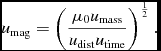 $$\begin{equation}
u_{\rm mag} = \left(\frac{\mu _{0} u_{\rm mass}}{u_{\rm dist} u_{\rm time}} \right)^{\frac{1}{2}}.
\end{equation}$$
$$\begin{equation}
u_{\rm mag} = \left(\frac{\mu _{0} u_{\rm mass}}{u_{\rm dist} u_{\rm time}} \right)^{\frac{1}{2}}.
\end{equation}$$
Converting the magnetic field in the code to physical units therefore only requires specifying μ0 in the relevant unit system. In particular, it avoids the differences between SI and cgs units in how the charge unit is defined, since μ0 is dimensionless and equal to 4π in cgs units but has dimensions that involve charge in SI units.
2.10.4. Tensile instability correction
The correction term f divB is necessary to avoid the tensile instability—a numerical instability where particles attract each other along field lines—in the regime where the magnetic pressure exceeds the gas pressure, that is, when plasma 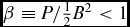 $\beta \equiv P / \frac{1}{2} B^2 < 1$ (Phillips & Monaghan Reference Phillips and Monaghan1985). The correction term is computed using the symmetric divergence operator (Børve et al. Reference Børve, Omang and Trulsen2001; Price Reference Price2012a; Tricco & Price Reference Tricco and Price2012)
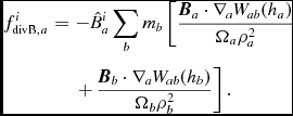 $$\begin{eqnarray}
f^{i}_{{\rm divB}, a} &=& -\hat{B}_{a}^{i} \sum _{b} m_{b} \left[ \frac{{\bm B}_{a} \cdot \nabla _{a} W_{ab} (h_{a})}{\Omega _{a} \rho _{a}^{2}} \right. \nonumber \\
&& \left. + \,\frac{{\bm B}_{b} \cdot \nabla _{a} W_{ab} (h_{b})}{\Omega _{b} \rho _{b}^{2}} \right].
\end{eqnarray}$$
$$\begin{eqnarray}
f^{i}_{{\rm divB}, a} &=& -\hat{B}_{a}^{i} \sum _{b} m_{b} \left[ \frac{{\bm B}_{a} \cdot \nabla _{a} W_{ab} (h_{a})}{\Omega _{a} \rho _{a}^{2}} \right. \nonumber \\
&& \left. + \,\frac{{\bm B}_{b} \cdot \nabla _{a} W_{ab} (h_{b})}{\Omega _{b} \rho _{b}^{2}} \right].
\end{eqnarray}$$
Since this term violates momentum conservation to the extent that the  $\nabla \cdot {\bm B}$ term is non-zero, several authors have proposed ways to minimise its effect. Børve et al. (Reference Børve, Omang and Trulsen2004) showed that stability could be achieved with $\hat{B}^i = \frac{1}{2} B^i$ and also proposed a scheme for scaling this term to zero for β > 1. Barnes, Kawata, & Wu (Reference Barnes, Kawata and Wu2012) similarly advocated using a factor of $\frac{1}{2}$ in this term. However, Tricco & Price (Reference Tricco and Price2012) showed that this could lead to problematic effects (their Figure 12). In Phantom, we use
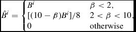 $$\begin{equation}
\hat{B}^i = \left\lbrace \arraycolsep5pt\begin{array}{@{}ll@{}}B^i & \beta < 2, \\
{[}(10 - \beta ) B^i]/8 & 2 < \beta < 10, \\
0 & \textrm {otherwise} \end{array}\right.
\end{equation}$$
$$\begin{equation}
\hat{B}^i = \left\lbrace \arraycolsep5pt\begin{array}{@{}ll@{}}B^i & \beta < 2, \\
{[}(10 - \beta ) B^i]/8 & 2 < \beta < 10, \\
0 & \textrm {otherwise} \end{array}\right.
\end{equation}$$
to provide numerical stability in the strong field regime while maintaining conservation of momentum when β > 10. This also helps to reduce errors in the MHD wave speed caused by the correction term (Iwasaki Reference Iwasaki2015).
2.10.5. Shock capturing
The shock capturing term in the momentum equation for MHD is identical to (39) and (40) except that the signal speed becomes (Price & Monaghan Reference Price and Monaghan2004a, Reference Price and Monaghan2005; Price Reference Price2012a)
 $$\begin{equation}
v_{{\rm sig}, a} = \alpha ^{\rm AV}_{a} v_{a} + \beta ^{\rm AV} \vert {\bm v}_{ab}\cdot \hat{\bm r}_{ab} \vert ,
\end{equation}$$
$$\begin{equation}
v_{{\rm sig}, a} = \alpha ^{\rm AV}_{a} v_{a} + \beta ^{\rm AV} \vert {\bm v}_{ab}\cdot \hat{\bm r}_{ab} \vert ,
\end{equation}$$
where
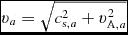 $$\begin{equation}
v_{a} = \sqrt{c^{2}_{{\rm s}, a} + v_{{\rm A}, a}^{2}}
\end{equation}$$
$$\begin{equation}
v_{a} = \sqrt{c^{2}_{{\rm s}, a} + v_{{\rm A}, a}^{2}}
\end{equation}$$
is the fast magnetosonic speed. Apart from this, the major difference to the hydrodynamic case is the addition of an artificial resistivity term to capture shocks and discontinuities in the magnetic field (i.e. current sheets). This is given by
 $$\begin{equation}
\mathcal {D}^{a}_{{\rm diss}} = \frac{\rho _{a}}{2} \sum _{b} m_{b} \left[ \frac{v^{B}_{{\rm sig}, a}}{\rho _{a}^{2}} \frac{F_{ab}(h_{a})}{\Omega _{a}} + \frac{v^{B}_{{\rm sig}, b}}{\rho _{b}^{2}} \frac{F_{ab}(h_{b})}{\Omega _{b}} \right]{\bm B}_{ab},
\end{equation}$$
$$\begin{equation}
\mathcal {D}^{a}_{{\rm diss}} = \frac{\rho _{a}}{2} \sum _{b} m_{b} \left[ \frac{v^{B}_{{\rm sig}, a}}{\rho _{a}^{2}} \frac{F_{ab}(h_{a})}{\Omega _{a}} + \frac{v^{B}_{{\rm sig}, b}}{\rho _{b}^{2}} \frac{F_{ab}(h_{b})}{\Omega _{b}} \right]{\bm B}_{ab},
\end{equation}$$
where vB sig, a is an appropriate signal speed (see below) multiplied by a dimensionless coefficient, αB. The corresponding contribution to the thermal energy from the resistivity term in (42) is given by
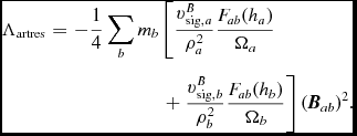 $$\begin{eqnarray}
\Lambda _{\rm artres} &= & - \frac{1}{4} \sum _{b} m_{b} \left[ \frac{v^{B}_{{\rm sig}, a}}{\rho _{a}^{2}} \frac{F_{ab}(h_{a})}{\Omega _{a}} \right. \nonumber \\
&& \left. \phantom{-\frac{1}{2}\sum _{b} m_{b}}+ \frac{v^{B}_{{\rm sig}, b}}{\rho _{b}^{2}} \frac{F_{ab}(h_{b})}{\Omega _{b}} \right] ({\bm B}_{ab})^{2}.
\end{eqnarray}$$
$$\begin{eqnarray}
\Lambda _{\rm artres} &= & - \frac{1}{4} \sum _{b} m_{b} \left[ \frac{v^{B}_{{\rm sig}, a}}{\rho _{a}^{2}} \frac{F_{ab}(h_{a})}{\Omega _{a}} \right. \nonumber \\
&& \left. \phantom{-\frac{1}{2}\sum _{b} m_{b}}+ \frac{v^{B}_{{\rm sig}, b}}{\rho _{b}^{2}} \frac{F_{ab}(h_{b})}{\Omega _{b}} \right] ({\bm B}_{ab})^{2}.
\end{eqnarray}$$
As with the artificial viscosity, (181) and (182) are the SPH representation of a physical resistivity term,  $\eta \nabla ^2 {\bm B}$, but with a coefficient that is proportional to resolution (Price & Monaghan Reference Price and Monaghan2004a). The resistive dissipation rate from the shock capturing term is given by
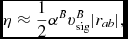 $$\begin{equation}
\eta \approx \frac{1}{2} \alpha ^{B} v_{\rm sig}^{B} \vert r_{ab} \vert ,
\end{equation}$$
$$\begin{equation}
\eta \approx \frac{1}{2} \alpha ^{B} v_{\rm sig}^{B} \vert r_{ab} \vert ,
\end{equation}$$
where |r ab|∝h.
2.10.6. Switch to reduce resistivity
Phantom previously used the method proposed by Tricco & Price (Reference Tricco and Price2013) to reduce the dissipation in the magnetic field away from shocks and discontinuities. The signal velocity, vB sig, was set equal to the magnetosonic speed [Equation (180)] multiplied by the dimensionless coefficient αB, which was set according to
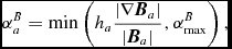 $$\begin{equation}
\alpha ^{B}_{a} = \min \left( h_{a} \frac{\vert \nabla {\bm B}_{a} \vert }{\vert {\bm B}_{a}\vert }, \alpha ^{B}_{\max }\right),
\end{equation}$$
$$\begin{equation}
\alpha ^{B}_{a} = \min \left( h_{a} \frac{\vert \nabla {\bm B}_{a} \vert }{\vert {\bm B}_{a}\vert }, \alpha ^{B}_{\max }\right),
\end{equation}$$
where αBmax = 1.0 by default and  $\vert \nabla {\bm B}_{a} \vert$ is the two-norm of the gradient tensor, i.e. the root mean square of all nine components of this tensor. Unlike the viscous dissipation, this is set based on the instantaneous values of h and ${\bm B}$ and there is no source/decay equation involved, as Tricco & Price (Reference Tricco and Price2013) found it to be unnecessary. Since αB is proportional to resolution, from (183), we see that this results in dissipation that is effectively second order (∝h 2). When individual particle timesteps were used, inactive particles retained their value of αB from the last timestep they were active.
More recently, we have found that a better approach, similar to that used for artificial conductivity, is to simply set αB = 1 for all particles and set the signal speed for artificial resistivity according to
 $$\begin{equation}
v_{\rm sig}^{B} = \vert {\bm v}_{ab} \times \hat{\bm r}_{ab} \vert .
\end{equation}$$
$$\begin{equation}
v_{\rm sig}^{B} = \vert {\bm v}_{ab} \times \hat{\bm r}_{ab} \vert .
\end{equation}$$
We find that this produces better results on all of our tests (Section 5.6), in particular, producing zero numerical dissipation on the current loop advection test (Section 5.6.5). As with the Tricco & Price (Reference Tricco and Price2013) switch, it gives second-order dissipation in the magnetic field (demonstrated in Section 5.6.1, Figure 26). This is now the default treatment for artificial resistivity in Phantom.
2.10.7. Conservation properties
The total energy when using MHD is given by
 $$\begin{equation}
E = \sum _{a} m_{a} \left( \frac{1}{2} v_{a}^{2} + u_{a} + \Phi _{a} + \frac{1}{2} \frac{B^{2}_{a}}{\mu _{0}\rho _{a}} \right).
\end{equation}$$
$$\begin{equation}
E = \sum _{a} m_{a} \left( \frac{1}{2} v_{a}^{2} + u_{a} + \Phi _{a} + \frac{1}{2} \frac{B^{2}_{a}}{\mu _{0}\rho _{a}} \right).
\end{equation}$$
Hence, total energy conservation, in the absence of divergence cleaning, corresponds to
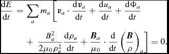 $$\begin{eqnarray}
\frac{{\rm d}E}{{\rm d}t} &=& \sum _{a} m_{a} \left[ {\bm v}_{a} \cdot \frac{{\rm d}{\bm v}_{a}}{{\rm d}t} + \frac{{\rm d}u_{a}}{{\rm d}t} + \frac{{\rm d} \Phi _{a}}{{\rm d}t} \right. \nonumber \\
&& +\, \left. \frac{{B}^{2}_{a}}{2 \mu _{0}\rho _{a}^{2}} \frac{{\rm d}\rho _{a}}{{\rm d}t} + \frac{{\bm B}_{a}}{ \mu _{0}} \cdot \frac{{\rm d}}{{\rm d}t} \left( \frac{{\bm B}}{\rho } \right)_a \right] = 0.
\end{eqnarray}$$
$$\begin{eqnarray}
\frac{{\rm d}E}{{\rm d}t} &=& \sum _{a} m_{a} \left[ {\bm v}_{a} \cdot \frac{{\rm d}{\bm v}_{a}}{{\rm d}t} + \frac{{\rm d}u_{a}}{{\rm d}t} + \frac{{\rm d} \Phi _{a}}{{\rm d}t} \right. \nonumber \\
&& +\, \left. \frac{{B}^{2}_{a}}{2 \mu _{0}\rho _{a}^{2}} \frac{{\rm d}\rho _{a}}{{\rm d}t} + \frac{{\bm B}_{a}}{ \mu _{0}} \cdot \frac{{\rm d}}{{\rm d}t} \left( \frac{{\bm B}}{\rho } \right)_a \right] = 0.
\end{eqnarray}$$
Neglecting the f divB correction term for the moment, substituting (171), (35), and (172) into (187) with the ideal MHD and shock capturing terms included demonstrates that the total energy is exactly conserved, using the same argument as the one given in Section 2.2.6 (detailed workings can be found in Price & Monaghan Reference Price and Monaghan2004b). The total linear momentum is also exactly conserved following a similar argument as in Section 2.2.11. However, the presence of the f divB correction term, though necessary for numerical stability, violates the conservation of both momentum and energy in the strong field regime (in the weak field regime, it is switched off and conservation is preserved). The severity of this non-conservation is related to the degree in which divergence errors are present in the magnetic field, hence inadequate divergence control (see below) usually manifests as a loss of momentum conservation in the code (see Tricco & Price Reference Tricco and Price2012, for details).
2.10.8. Divergence cleaning
We adopt the ‘constrained’ hyperbolic/parabolic divergence cleaning algorithm described by Tricco & Price (Reference Tricco and Price2012) and Tricco et al. (Reference Tricco, Price and Bate2016a) to preserve the divergence-free condition on the magnetic field. This formulation addresses a number of issues with earlier formulations by Dedner et al. (Reference Dedner, Kemm, Kröner, Munz, Schnitzer and Wesenberg2002) and Price & Monaghan (Reference Price and Monaghan2005).
The main idea of the scheme is to propagate divergence errors according to a damped wave equation (Dedner et al. Reference Dedner, Kemm, Kröner, Munz, Schnitzer and Wesenberg2002; Price & Monaghan Reference Price and Monaghan2005). This is facilitated by introducing a new scalar field, ψ, which is coupled to the magnetic field in (167) and evolved according to (168).
Tricco et al. (Reference Tricco, Price and Bate2016a) generalised the method of Dedner et al. (Reference Dedner, Kemm, Kröner, Munz, Schnitzer and Wesenberg2002) to include the case where the hyperbolic wave speed, c h, varies in time and space. This is the approach we use in Phantom. The resulting ‘generalised wave equation’ may be derived by combining the relevant term in (167) with (168) to give (Tricco et al. Reference Tricco, Price and Bate2016a)
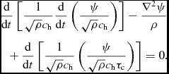 $$\begin{eqnarray}
&&\frac{{\rm d}}{{\rm d}t} \left[ \frac{1}{\sqrt{\rho } c_{\rm h}}\frac{{\rm d}}{{\rm d}t} \left( \frac{\psi }{\sqrt{\rho } c_{\rm h}} \right) \right] - \frac{\nabla ^{2} \psi }{\rho } \nonumber \\
&&\quad +\, \frac{{\rm d}}{{\rm d}t} \left[ \frac{1}{\sqrt{\rho } c_{\rm h}} \left(\frac{\psi }{\sqrt{\rho }c_{\rm h}\tau _{\rm c}}\right) \right] = 0.
\end{eqnarray}$$
$$\begin{eqnarray}
&&\frac{{\rm d}}{{\rm d}t} \left[ \frac{1}{\sqrt{\rho } c_{\rm h}}\frac{{\rm d}}{{\rm d}t} \left( \frac{\psi }{\sqrt{\rho } c_{\rm h}} \right) \right] - \frac{\nabla ^{2} \psi }{\rho } \nonumber \\
&&\quad +\, \frac{{\rm d}}{{\rm d}t} \left[ \frac{1}{\sqrt{\rho } c_{\rm h}} \left(\frac{\psi }{\sqrt{\rho }c_{\rm h}\tau _{\rm c}}\right) \right] = 0.
\end{eqnarray}$$
When c h, ρ, τc, and the fluid velocity are constant, this reduces to the usual damped wave equation in the form
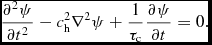 $$\begin{equation}
\frac{\partial ^{2} \psi }{\partial t^{2}} - c_{\rm h}^{2} \nabla ^{2} \psi + \frac{1}{\tau _{\rm c}} \frac{\partial \psi }{\partial t} = 0.
\end{equation}$$
$$\begin{equation}
\frac{\partial ^{2} \psi }{\partial t^{2}} - c_{\rm h}^{2} \nabla ^{2} \psi + \frac{1}{\tau _{\rm c}} \frac{\partial \psi }{\partial t} = 0.
\end{equation}$$
The same equation holds for the evolution of  ${\nabla \cdot {\bm B}}$ itself, i.e.
 $$\begin{equation}
\frac{\partial ^{2} (\nabla \cdot {\bm B})}{\partial t^{2}} - c_{\rm h}^{2} \nabla ^{2} (\nabla \cdot {\bm B}) + \frac{1}{\tau _{\rm c}} \frac{\partial (\nabla \cdot {\bm B})}{\partial t} = 0,
\end{equation}$$
$$\begin{equation}
\frac{\partial ^{2} (\nabla \cdot {\bm B})}{\partial t^{2}} - c_{\rm h}^{2} \nabla ^{2} (\nabla \cdot {\bm B}) + \frac{1}{\tau _{\rm c}} \frac{\partial (\nabla \cdot {\bm B})}{\partial t} = 0,
\end{equation}$$
from which it is clear that c h represents the speed at which divergence errors are propagated and τc is the decay timescale over which divergence errors are removed.
Tricco & Price (Reference Tricco and Price2012) formulated a ‘constrained’ SPMHD implementation of hyperbolic/parabolic cleaning which guarantees numerical stability of the cleaning. The constraint imposed by Tricco & Price (Reference Tricco and Price2012) is that, in the absence of damping, any energy removed from the magnetic field during cleaning must be conserved by the scalar field, ψ. This enforces particular choices of numerical operators for  $\nabla \cdot {\bm B}$ and ∇ψ in (172) and (173), respectively, in particular that they form a conjugate pair of difference and symmetric derivative operators. This guarantees that the change of magnetic energy is negative definite in the presence of the parabolic term (see below).
In Phantom, we set the cleaning speed, c h, equal to the fast magnetosonic speed [Equation (180)] so that its timestep constraint is satisfied already by (72), as recommended by Tricco & Price (Reference Tricco and Price2013). The decay timescale is set according to
 $$\begin{equation}
\tau ^a_{\rm c} \equiv \frac{h_a}{\sigma _{\rm c} c_{{\rm h},a}},
\end{equation}$$
$$\begin{equation}
\tau ^a_{\rm c} \equiv \frac{h_a}{\sigma _{\rm c} c_{{\rm h},a}},
\end{equation}$$
where the dimensionless factor σc sets the ratio of parabolic to hyperbolic cleaning. This is set to σc = 1.0 by default, which was empirically determined by Tricco & Price (Reference Tricco and Price2012) to provide optimal reduction of divergence errors in three dimensions.
The divergence cleaning dissipates energy from the magnetic field at a rate given by (Tricco & Price Reference Tricco and Price2012)
 $$\begin{equation}
\left(\frac{{\rm d} E}{{\rm d}t}\right)_{\rm cleaning} = -\sum _{a} m_{a} \frac{\psi ^{2}_{a}}{\mu _{0} \rho _{a} c_{{\rm h},a}^{2} \tau ^{a}_{\rm c}}.
\end{equation}$$
$$\begin{equation}
\left(\frac{{\rm d} E}{{\rm d}t}\right)_{\rm cleaning} = -\sum _{a} m_{a} \frac{\psi ^{2}_{a}}{\mu _{0} \rho _{a} c_{{\rm h},a}^{2} \tau ^{a}_{\rm c}}.
\end{equation}$$
In general, this is so small compared to other dissipation terms (e.g. resistivity for shock capturing) that it is not worth monitoring (Tricco et al. Reference Tricco, Price and Bate2016a). This energy is not added as heat, but simply removed from the calculation.
2.10.9. Monitoring of divergence errors and over-cleaning
The divergence cleaning algorithm is guaranteed to either conserve or dissipate magnetic energy, and cleans divergence errors to a sufficient degree for most applications. However, the onus is on the user to ensure that divergence errors are not affecting simulation results. This may be monitored by the dimensionless quantity
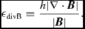 $$\begin{equation}
\epsilon _{\rm divB} \equiv \frac{h\vert \nabla \cdot {\bm B}\vert }{\vert {\bm B} \vert }.
\end{equation}$$
$$\begin{equation}
\epsilon _{\rm divB} \equiv \frac{h\vert \nabla \cdot {\bm B}\vert }{\vert {\bm B} \vert }.
\end{equation}$$
The maximum and mean values of this quantity should be used to check the fidelity of simulations that include magnetic fields. A good rule-of-thumb is that the mean should remain ≲ 10−2 for the simulation to remain qualitatively unaffected by divergence errors.
The cleaning wave speed can be arbitrarily increased to improve the effectiveness of the divergence cleaning according to
 $$\begin{equation}
c_{{\rm h}, a} = f_{\rm clean} v_a ,
\end{equation}$$
$$\begin{equation}
c_{{\rm h}, a} = f_{\rm clean} v_a ,
\end{equation}$$
where f clean is an ‘over-cleaning’ factor (by default, f clean = 1, i.e. no ‘over-cleaning’). Tricco et al. (Reference Tricco, Price and Bate2016a) showed that increasing f clean leads to further reduction in divergence errors, without affecting the quality of obtained results, but with an accompanying computational expense associated with a reduction in the timestep size.
2.11. Non-ideal magnetohydrodynamics
Phantom implements non-ideal MHD including terms for Ohmic resistivity, ambipolar (ion-neutral) diffusion and the Hall effect. Algorithms and tests are taken from Wurster, Price, & Ayliffe (Reference Wurster, Price and Ayliffe2014) and Wurster, Price, & Bate (Reference Wurster, Price and Bate2016). See Wurster et al. (Reference Wurster, Price and Bate2016, Reference Wurster, Price and Bate2017) and Wurster, Bate, & Price (Reference Wurster, Bate and Price2018) for recent applications. Our formulation of non-ideal SPMHD in Phantom is simpler than the earlier formulation proposed by Hosking & Whitworth (Reference Hosking and Whitworth2004) because we consider only one set of particles, representing a mixture of charged and uncharged species. Ours is similar to the implementation by Tsukamoto, Iwasaki, & Inutsuka (Reference Tsukamoto, Iwasaki and Inutsuka2013) and Tsukamoto et al. (Reference Tsukamoto, Iwasaki, Okuzumi, Machida and Inutsuka2015).
2.11.1. Equations of non-ideal MHD
We assume the strong coupling or ‘heavy ion’ approximation (see e.g. Wardle & Ng Reference Wardle and Ng1999; Shu et al. Reference Shu, Galli, Lizano and Cai2006; Pandey & Wardle Reference Pandey and Wardle2008), which neglects ion pressure and assumes ρi ≪ ρn, where the subscripts i and n refer to the ionised and neutral fluids, respectively. In this case, (167) contains three additional terms in the form
 $$\begin{equation}
\frac{{\rm d}}{{\rm d}t} \left( \frac{{\bm B}}{\rho } \right)_{\rm nimhd} = -\frac{1}{\rho } \nabla \times \left[ \frac{\bm J}{\sigma _e} + \frac{{\bm J} \times {\bm B}}{e n_e} - \frac{({\bm J} \times {\bm B}) \times {\bm B}}{\gamma _{\rm AD} \rho _i}\right],
\end{equation}$$
$$\begin{equation}
\frac{{\rm d}}{{\rm d}t} \left( \frac{{\bm B}}{\rho } \right)_{\rm nimhd} = -\frac{1}{\rho } \nabla \times \left[ \frac{\bm J}{\sigma _e} + \frac{{\bm J} \times {\bm B}}{e n_e} - \frac{({\bm J} \times {\bm B}) \times {\bm B}}{\gamma _{\rm AD} \rho _i}\right],
\end{equation}$$
where σe is the electrical conductivity, n e is the number density of electrons, e is the charge on an electron, and γAD is the collisional coupling constant between ions and neutrals (Pandey & Wardle Reference Pandey and Wardle2008). We write this in the form
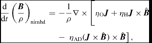 $$\begin{eqnarray}
\frac{{\rm d}}{{\rm d}t} \left( \frac{{\bm B}}{\rho } \right)_{\rm nimhd} &=& -\frac{1}{\rho } \nabla \times \bigg [ \eta _{\rm O} {\bm J} + \eta _{\rm H} {\bm J} \times \hat{\bm B} \nonumber \\
&& -\, \left. \eta _{\rm AD} ({\bm J} \times \hat{\bm B}) \times \hat{\bm B} \right],
\end{eqnarray}$$
$$\begin{eqnarray}
\frac{{\rm d}}{{\rm d}t} \left( \frac{{\bm B}}{\rho } \right)_{\rm nimhd} &=& -\frac{1}{\rho } \nabla \times \bigg [ \eta _{\rm O} {\bm J} + \eta _{\rm H} {\bm J} \times \hat{\bm B} \nonumber \\
&& -\, \left. \eta _{\rm AD} ({\bm J} \times \hat{\bm B}) \times \hat{\bm B} \right],
\end{eqnarray}$$
where  $\hat{\bm B}$ is the unit vector in the direction of ${\bm B}$ such that ηO, ηAD, and ηHall are the coefficients for resistive and ambipolar diffusion and the Hall effect, respectively, each with dimensions of area per unit time.
To conserve energy, we require the corresponding resistive and ambipolar heating terms in the thermal energy equation in the form
 $$\begin{equation}
\left( \frac{{\rm d}u}{{\rm d}t}\right)_{\rm nimhd} = \frac{ \eta _{\rm O}}{\rho } J^2 + \frac{\eta _{\rm AD}}{\rho } \left[ J^2 - ({\bm J}\cdot {\hat{\bm B}})^2\right].
\end{equation}$$
$$\begin{equation}
\left( \frac{{\rm d}u}{{\rm d}t}\right)_{\rm nimhd} = \frac{ \eta _{\rm O}}{\rho } J^2 + \frac{\eta _{\rm AD}}{\rho } \left[ J^2 - ({\bm J}\cdot {\hat{\bm B}})^2\right].
\end{equation}$$
The Hall term is non-dissipative, being dispersive rather than diffusive, so does not enter the energy equation.
We currently neglect the ‘Biermann battery’ term (Biermann Reference Biermann1950) proportional to ∇P e/(en e) in our non-ideal MHD implementation, both because it is thought to be negligible in the interstellar medium (Pandey & Wardle Reference Pandey and Wardle2008) and because numerical implementations can produce incorrect results (Graziani et al. Reference Graziani, Tzeferacos, Lee, Lamb, Weide, Fatenejad and Miller2015). This term is mainly important in generating seed magnetic fields for subsequent dynamo processes (e.g. Khomenko et al. Reference Khomenko, Vitas, Collados and de Vicente2017).
2.11.2. Discrete equations
Our main constraint is that the numerical implementation of the non-ideal MHD terms should exactly conserve energy, which is achieved by discretising in the form (Wurster et al. Reference Wurster, Price and Ayliffe2014)
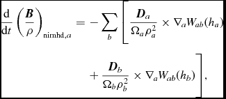 $$\begin{eqnarray}
\frac{{\rm d}}{{\rm d}t} \left( \frac{{\bm B}}{\rho } \right)_{{\rm nimhd},a} &=& - \sum _b \Bigg [ \frac{{\bm D}_a}{\Omega _a \rho _a^2} \times \nabla _a W_{ab} (h_a) \nonumber \\
&&+\, \frac{{\bm D}_b}{\Omega _b \rho _b^2} \times \nabla _a W_{ab} (h_b) \Bigg ],
\end{eqnarray}$$
$$\begin{eqnarray}
\frac{{\rm d}}{{\rm d}t} \left( \frac{{\bm B}}{\rho } \right)_{{\rm nimhd},a} &=& - \sum _b \Bigg [ \frac{{\bm D}_a}{\Omega _a \rho _a^2} \times \nabla _a W_{ab} (h_a) \nonumber \\
&&+\, \frac{{\bm D}_b}{\Omega _b \rho _b^2} \times \nabla _a W_{ab} (h_b) \Bigg ],
\end{eqnarray}$$
where
 $$\begin{equation}
{\bm D} = -\eta _{\rm O} {\bm J} - \eta _{\rm H} ({\bm J} \times \hat{\bm B}) + \eta _{\rm AD} [({\bm J} \times \hat{\bm B}) \times \hat{\bm B}].
\end{equation}$$
$$\begin{equation}
{\bm D} = -\eta _{\rm O} {\bm J} - \eta _{\rm H} ({\bm J} \times \hat{\bm B}) + \eta _{\rm AD} [({\bm J} \times \hat{\bm B}) \times \hat{\bm B}].
\end{equation}$$
The corresponding term in the energy equation is given by
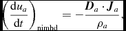 $$\begin{equation}
\left( \frac{{\rm d}u_a}{{\rm d}t}\right)_{\rm nimhd} = - \frac{{\bm D}_a \cdot {\bm J}_a}{\rho _a},
\end{equation}$$
$$\begin{equation}
\left( \frac{{\rm d}u_a}{{\rm d}t}\right)_{\rm nimhd} = - \frac{{\bm D}_a \cdot {\bm J}_a}{\rho _a},
\end{equation}$$
where the magnetic current density is computed alongside the density evaluation according to
 $$\begin{equation}
{\bm J} = \frac{1}{\Omega _a\rho _a} \sum _b m_b ({\bm B}_a - {\bm B}_b) \times \nabla _a W_{ab} (h_a).
\end{equation}$$
$$\begin{equation}
{\bm J} = \frac{1}{\Omega _a\rho _a} \sum _b m_b ({\bm B}_a - {\bm B}_b) \times \nabla _a W_{ab} (h_a).
\end{equation}$$
Non-ideal MHD therefore utilises a ‘two first derivatives’ approach, similar to the formulation of physical viscosity described in Section 2.7.1. This differs from the ‘direct second derivatives’ approach used for our artificial resistivity term, and in previous formulations of physical resistivity (Bonafede et al. Reference Bonafede, Dolag, Stasyszyn, Murante and Borgani2011). In practice, the differences are usually minor. Our main reason for using two first derivatives for non-ideal MHD is that it is easier to incorporate the Hall effect and ambipolar diffusion terms.
2.11.3. Computing the non-ideal MHD coefficients
To self-consistently compute the coefficients ηO, ηH, and ηAD from the local gas properties, we use the nicil library (Wurster Reference Wurster2016) for cosmic ray ionisation chemistry and thermal ionisation. We refer the reader to Wurster (Reference Wurster2016) and Wurster et al. (Reference Wurster, Price and Bate2016) for details, since this is maintained and versioned as a separate package.
2.11.4. Timestepping
With explicit timesteps, the timestep is constrained in a similar manner to other terms, using
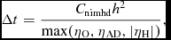 $$\begin{equation}
\Delta t = \frac{C_{\rm nimhd} h^2}{\max (\eta _{\rm O},\eta _{\rm AD}, \vert \eta _{\rm H}\vert )},
\end{equation}$$
$$\begin{equation}
\Delta t = \frac{C_{\rm nimhd} h^2}{\max (\eta _{\rm O},\eta _{\rm AD}, \vert \eta _{\rm H}\vert )},
\end{equation}$$
where C nimhd = 1/(2π) by default. This can prove prohibitive, so we employ the so-called ‘super-timestepping’ algorithm from Alexiades, Amiez, & Gremaud (Reference Alexiades, Amiez and Gremaud1996) to relax the stability criterion for the Ohmic and ambipolar terms (only). The implementation is described in detail in Wurster et al. (Reference Wurster, Price and Bate2016). Currently, the Hall effect is always timestepped explicitly in the code.
2.12. Self-gravity
Phantom includes self-gravity between particles. By self-gravity, we mean a solution to Poisson’s equation
 $$\begin{equation}
\nabla ^{2} \Phi = 4\pi G \rho ({\bm r}),
\end{equation}$$
$$\begin{equation}
\nabla ^{2} \Phi = 4\pi G \rho ({\bm r}),
\end{equation}$$
where Φ is the gravitational potential and ρ represents a continuous fluid density. The corresponding acceleration term in the equation of motion is
 $$\begin{equation}
{\bm a}_{\rm selfgrav} = -\nabla \Phi .
\end{equation}$$
$$\begin{equation}
{\bm a}_{\rm selfgrav} = -\nabla \Phi .
\end{equation}$$
Since (203) is an elliptic equation, implying instant action, it requires a global solution. This solution is obtained in Phantom by splitting the acceleration into ‘short-range’ and ‘long-range’ contributions.
 $$\begin{equation}
{\bm a}^{a}_{\rm selfgrav} = {\bm a}^{a}_{\rm short} + {\bm a}^{a}_{\rm long} ,
\end{equation}$$
$$\begin{equation}
{\bm a}^{a}_{\rm selfgrav} = {\bm a}^{a}_{\rm short} + {\bm a}^{a}_{\rm long} ,
\end{equation}$$
where the ‘short-range’ interaction is computed by direct summation over nearby particles, and the ‘long-range’ interaction is computed by hierarchical grouping of particles using the kd-tree.
The distance at which the gravitational acceleration is treated as ‘short-’ or ‘long-range’ is determined for each node–node pair, n–m, either by the tree opening criterion,
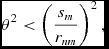 $$\begin{equation}
\theta ^{2} < \left(\frac{s_{m}}{r_{nm}}\right)^{2},
\end{equation}$$
$$\begin{equation}
\theta ^{2} < \left(\frac{s_{m}}{r_{nm}}\right)^{2},
\end{equation}$$
where 0 ⩽ θ ⩽ 1 is the tree opening parameter, or by nodes whose smoothing spheres intersect,
 $$\begin{equation}
r_{nm}^{2} < \left[s_{n} + s_{m} + \max (R_{\rm kern} h_{\max }^{n}, R_{\rm kern} h_{\max }^{m})\right]^{2}.
\end{equation}$$
$$\begin{equation}
r_{nm}^{2} < \left[s_{n} + s_{m} + \max (R_{\rm kern} h_{\max }^{n}, R_{\rm kern} h_{\max }^{m})\right]^{2}.
\end{equation}$$
Here, s is the node size, which is the minimum radius about the centre of mass that contains all the particles in the node, and h max is the maximum smoothing length of the particles within the node. Node pairs satisfying either of these criteria have the particles contained within them added to a trial neighbour list, used for computing the short-range gravitational acceleration. Setting θ = 0, therefore, leads to the gravitational acceleration computed entirely as ‘short-range’, that is, only via direction summation, while θ = 1 gives the fastest possible, but least accurate, gravitational force evaluation. The code default is θ = 0.5.
2.12.1. Short-range interaction
How to solve (203) on particles is one of the most widely misunderstood problems in astrophysics. In SPH or collisionless N-body simulations (i.e. stars and dark matter), the particles do not represent physical point-mass particles, but rather interpolation points in a density field that is assumed to be continuous. Hence, one needs to first reconstruct the density field on the particles, then solve (203) in a manner which is consistent with this (e.g. Hernquist & Barnes Reference Hernquist and Barnes1990).
How to do this consistently using a spatially adaptive softening length was demonstrated by Price & Monaghan (Reference Price and Monaghan2007), since an obvious choice is to use the iterative kernel summation in (3) to both reconstruct the density field and set the softening length, i.e.Footnote 6
 $$\begin{equation}
\rho _{a} = \sum _{b} m_{b} W_{ab} (\epsilon _{a}); \hspace{14.22636pt} \epsilon _{a} = h_{\rm fac} (m_{a}/\rho _{a})^{1/3}.
\end{equation}$$
$$\begin{equation}
\rho _{a} = \sum _{b} m_{b} W_{ab} (\epsilon _{a}); \hspace{14.22636pt} \epsilon _{a} = h_{\rm fac} (m_{a}/\rho _{a})^{1/3}.
\end{equation}$$
It can then be shown that the gravitational potential consistent with this choice is given by
 $$\begin{equation}
\Phi _{a} = -G \sum _{b} m_{b} \phi (\vert {\bm r}_{a} - {\bm r}_{b} \vert , \epsilon _{a}),
\end{equation}$$
$$\begin{equation}
\Phi _{a} = -G \sum _{b} m_{b} \phi (\vert {\bm r}_{a} - {\bm r}_{b} \vert , \epsilon _{a}),
\end{equation}$$
where ϕ is the softening kernel derived from the density kernel via Poisson’s equation (Section 2.12.2). For a variable smoothing length, energy conservation necessitates taking an average of the kernels, i.e.
 $$\begin{equation}
\Phi _{a} = -G \sum _{b} m_{b} \left[ \frac{\phi _{ab}(\epsilon _{a}) + \phi _{ab}(\epsilon _{b})}{2} \right].
\end{equation}$$
$$\begin{equation}
\Phi _{a} = -G \sum _{b} m_{b} \left[ \frac{\phi _{ab}(\epsilon _{a}) + \phi _{ab}(\epsilon _{b})}{2} \right].
\end{equation}$$
Price & Monaghan (Reference Price and Monaghan2007) showed how the equations of motion could then be derived from a Lagrangian in order to take account of the softening length gradient terms, giving equations of motion in the form
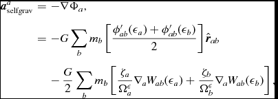 $$\begin{eqnarray}
\hspace*{-15pt}{\bm a}^{a}_{\rm selfgrav} &= & -\nabla \Phi _{a}, \nonumber \\
\hspace*{-15pt}&=& -G \sum _{b} m_{b} \left[ \frac{\phi ^{\prime }_{ab}(\epsilon _{a}) + \phi ^{\prime }_{ab}(\epsilon _{b})}{2}\right] \hat{\bm r}_{ab} \nonumber \\
\hspace*{-15pt}&& -\,\frac{G}{2} \sum _{b} m_{b} \left[ \frac{\zeta _{a}}{\Omega ^{\epsilon }_{a}} \nabla _{a} W_{ab} (\epsilon _{a}) + \frac{\zeta _{b}}{\Omega ^{\epsilon }_{b}} \nabla _{a} W_{ab} (\epsilon _{b})\right],
\end{eqnarray}$$
$$\begin{eqnarray}
\hspace*{-15pt}{\bm a}^{a}_{\rm selfgrav} &= & -\nabla \Phi _{a}, \nonumber \\
\hspace*{-15pt}&=& -G \sum _{b} m_{b} \left[ \frac{\phi ^{\prime }_{ab}(\epsilon _{a}) + \phi ^{\prime }_{ab}(\epsilon _{b})}{2}\right] \hat{\bm r}_{ab} \nonumber \\
\hspace*{-15pt}&& -\,\frac{G}{2} \sum _{b} m_{b} \left[ \frac{\zeta _{a}}{\Omega ^{\epsilon }_{a}} \nabla _{a} W_{ab} (\epsilon _{a}) + \frac{\zeta _{b}}{\Omega ^{\epsilon }_{b}} \nabla _{a} W_{ab} (\epsilon _{b})\right],
\end{eqnarray}$$
where Ωε and ζ are correction terms necessary for energy conservation, with Ω as in (5) but with h replaced by ε, and ζ defined as
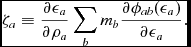 $$\begin{equation}
\zeta _{a} \equiv \frac{\partial \epsilon _{a}}{\partial \rho _{a}} \sum _{b} m_{b} \frac{\partial \phi _{ab}(\epsilon _{a})}{\partial \epsilon _{a}}.
\end{equation}$$
$$\begin{equation}
\zeta _{a} \equiv \frac{\partial \epsilon _{a}}{\partial \rho _{a}} \sum _{b} m_{b} \frac{\partial \phi _{ab}(\epsilon _{a})}{\partial \epsilon _{a}}.
\end{equation}$$
The above formulation satisfies all of the conservation properties, namely conservation of linear momentum, angular momentum, and energy.
The short-range acceleration is evaluated for each particle in the leaf node n by summing (211) over the trial neighbour list obtained by node–node pairs that satisfy either of the criteria in (206) or (207). For particle pairs separated outside the softening radius of either particle, the short range interaction reduces to
 $$\begin{equation}
{\bm a}^{a}_{\rm short, r > R_{\rm kern}\epsilon } = -G \sum _{b} m_{b} \frac{ {\bm r}_{a} - {\bm r}_{b}}{\vert {\bm r}_{a} - {\bm r}_{b}\vert ^{3}}.
\end{equation}$$
$$\begin{equation}
{\bm a}^{a}_{\rm short, r > R_{\rm kern}\epsilon } = -G \sum _{b} m_{b} \frac{ {\bm r}_{a} - {\bm r}_{b}}{\vert {\bm r}_{a} - {\bm r}_{b}\vert ^{3}}.
\end{equation}$$
We use this directly for such pairs to avoid unnecessary evaluations of the softening kernel.
It is natural in SPH to set the gravitational softening length equal to the smoothing length ε = h, since both derive from the same density estimate. Indeed, Bate & Burkert (Reference Bate and Burkert1997) showed that this is a crucial requirement to resolve gas fragmentation correctly. For pure N-body calculations, Price & Monaghan (Reference Price and Monaghan2007) also showed that setting the (variable) softening length in the same manner as the SPH smoothing length (Sections 2.1.3–2.1.4) results in a softening that is always close to the ‘optimal’ fixed softening length (Merritt Reference Merritt1996; Athanassoula et al. Reference Athanassoula, Fady, Lambert and Bosma2000; Dehnen Reference Dehnen2001). In collisionless N-body simulations, this has been found to increase the resolving power, giving results at lower resolution comparable to those obtained at higher resolution with a fixed softening length (Bagla & Khandai Reference Bagla and Khandai2009; Iannuzzi & Dolag Reference Iannuzzi and Dolag2011). It also avoids the problem of how to ‘choose’ the softening length, negating the need for ‘rules of thumb’ such as the one given by Springel (Reference Springel2005) where the softening length is chosen to be 1/40 of the average particle spacing in the initial conditions.
2.12.2. Functional form of the softening kernel
The density kernel and softening potential kernel are related using Poisson’s equation (203), i.e.
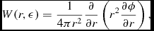 $$\begin{equation}
W(r, \epsilon ) = \frac{1}{4\pi r^{2}} \frac{\partial }{\partial r} \left( r^{2} \frac{\partial \phi }{\partial r} \right),
\end{equation}$$
$$\begin{equation}
W(r, \epsilon ) = \frac{1}{4\pi r^{2}} \frac{\partial }{\partial r} \left( r^{2} \frac{\partial \phi }{\partial r} \right),
\end{equation}$$
where  $r \equiv \vert {\bm r} - {\bm r}^{\prime }\vert$. Integrating this equation gives the softening kernels used for the force and gravitational potential. As with the standard kernel functions (Section 2.1.5), we define the potential and force kernels in terms of dimensionless functions of the scaled interparticle separation, q ≡ r/h, according to
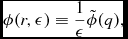 $$\begin{eqnarray}
\phi (r, \epsilon ) \equiv \frac{1}{\epsilon } \tilde{\phi } (q),
\end{eqnarray}$$
$$\begin{eqnarray}
\phi (r, \epsilon ) \equiv \frac{1}{\epsilon } \tilde{\phi } (q),
\end{eqnarray}$$
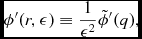 $$\begin{eqnarray}
\phi ^{\prime }(r, \epsilon ) \equiv \frac{1}{\epsilon ^{2}} \tilde{\phi }^{\prime } (q),
\end{eqnarray}$$
$$\begin{eqnarray}
\phi ^{\prime }(r, \epsilon ) \equiv \frac{1}{\epsilon ^{2}} \tilde{\phi }^{\prime } (q),
\end{eqnarray}$$
where the dimensionless force kernel is obtained from the density kernel f(q) (Section 2.1.5–2.1.6) using
 $$\begin{equation}
\tilde{\phi }^{\prime } (q) = \frac{4\pi }{q^{2}} C_{\rm norm} \int f(q^{\prime }) q^{\prime 2} {\rm d}q^{\prime },
\end{equation}$$
$$\begin{equation}
\tilde{\phi }^{\prime } (q) = \frac{4\pi }{q^{2}} C_{\rm norm} \int f(q^{\prime }) q^{\prime 2} {\rm d}q^{\prime },
\end{equation}$$
with the integration constant set such that 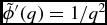 $\tilde{\phi }^{\prime }(q) = 1/q^{2}$ at q = R kern. The potential function is
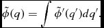 $$\begin{equation}
\tilde{\phi }(q) = \int \tilde{\phi }^{\prime }(q^{\prime }) dq^{\prime }.
\end{equation}$$
$$\begin{equation}
\tilde{\phi }(q) = \int \tilde{\phi }^{\prime }(q^{\prime }) dq^{\prime }.
\end{equation}$$
The derivative of ϕ with respect to ε required in (212) is also written in terms of a dimensionless function, i.e.
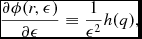 $$\begin{equation}
\frac{\partial \phi (r,\epsilon )}{\partial \epsilon } \equiv \frac{1}{\epsilon ^{2}} h(q),
\end{equation}$$
$$\begin{equation}
\frac{\partial \phi (r,\epsilon )}{\partial \epsilon } \equiv \frac{1}{\epsilon ^{2}} h(q),
\end{equation}$$
where from differentiating (215), we have
 $$\begin{equation}
h(q) = -\tilde{\phi }(q) - q\tilde{\phi }^{\prime }(q).
\end{equation}$$
$$\begin{equation}
h(q) = -\tilde{\phi }(q) - q\tilde{\phi }^{\prime }(q).
\end{equation}$$
Included in the Phantom source code is a Python script using the sympy library to solve (217), (218), and (220) using symbolic integration to obtain the softening kernel from the density kernel. This makes it straightforward to obtain the otherwise laborious expressions needed for each kernel [expressions for the cubic spline kernel are in Appendix A of Price & Monaghan (Reference Price and Monaghan2007) and for the quintic spline in Appendix A of Hubber et al. (Reference Hubber, Batty, McLeod and Whitworth2011)]. Figure 3 shows the functional form of the softening kernels for each of the kernels available in Phantom. The kernel function f(q) is shown for comparison (top row in each case).
Functional form of the softening kernel functions −ϕ(r, h) and ϕ′(r, h) used to compute the gravitational force in Phantom, shown for each of the available kernel functions w(r, h) (see Figure 1). Dotted lines show the functional form of the unsoftened potential (−1/r) and force (1/r 2) for comparison.
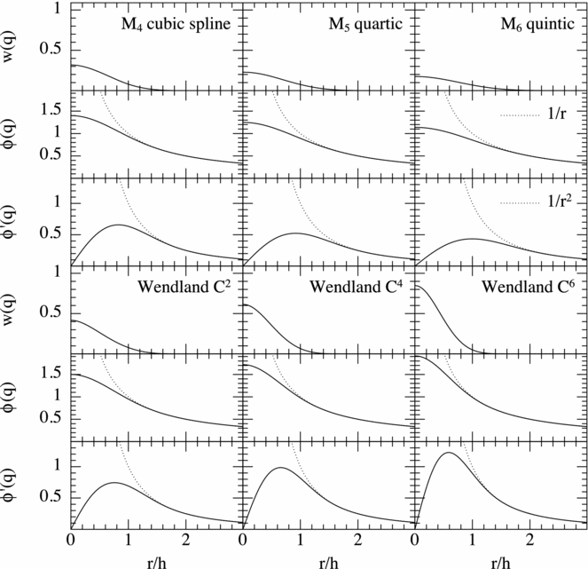
2.12.3. Softening of gravitational potential due to stars, dark matter, and dust
In the presence of collisionless components (e.g. stars, dark matter, and dust), we require estimates of the density in order to set the softening lengths for each component. We follow the generalisation of the SPH density estimate to multi-fluid systems described by Laibe & Price (Reference Laibe and Price2012a) where the density (and hence the softening length and Ωε) for each component is computed in the usual iterative manner (Section 2.1.4), but using only neighbours of the same type (c.f. Section 2.13.3). That is, the softening length for stars is determined based on the local density of stars, the softening length for dark matter is based on the local density of dark matter particles, and so on. The gravitational interaction both within each type and between different types is then computed using (211). This naturally symmetrises the softening between different types, ensuring that momentum, angular momentum, and energy are conserved.
2.12.4. Long-range interaction
At long range, that is r > R kernεa and r > R kernεb, the second term in (211) tends to zero since ζ = 0 for q ⩾ R kern, while the first term simply becomes 1/r 2. Computing this via direct summation would have an associated  $\mathcal {O}(N^{2})$ computational cost, thus we adopt the usual practice of using the kd-tree to reduce this cost to $\mathcal {O}(N\log N)$.
The main optimisation in Phantom compared to a standard tree code (e.g. Hernquist & Katz Reference Hernquist and Katz1989; Benz et al. Reference Benz, Cameron, Press and Bowers1990) is that we compute the long-range gravitational interaction once per leaf-node rather than once per-particle and that we use Cartesian rather than spherical multipole expansions to enable this (Dehnen Reference Dehnen2000b; Gafton & Rosswog Reference Gafton and Rosswog2011).
The long-range acceleration on a given leaf node n consists of a sum over distant nodes m that satisfy neither (206) nor (207).
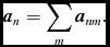 $$\begin{equation}
{\bm a}_{n} = \sum _{m} {\bm a}_{nm}.
\end{equation}$$
$$\begin{equation}
{\bm a}_{n} = \sum _{m} {\bm a}_{nm}.
\end{equation}$$
The acceleration along the node centres, between a given pair n and m, is given (using index notation) by
 $$\begin{equation}
a^{i}_{nm} = -\frac{GM_{m}}{r^{3}} r^{i} + \frac{1}{r^{4}} \left(\hat{r}^{k} Q^{m}_{ik} - \frac{5}{2} \hat{r}^{i} \mathcal {Q}^{m} \right),
\end{equation}$$
$$\begin{equation}
a^{i}_{nm} = -\frac{GM_{m}}{r^{3}} r^{i} + \frac{1}{r^{4}} \left(\hat{r}^{k} Q^{m}_{ik} - \frac{5}{2} \hat{r}^{i} \mathcal {Q}^{m} \right),
\end{equation}$$
where ri ≡ xin − xim is the relative position vector,  $\hat{r}$ is the corresponding unit vector, M m is the total mass in node m, Qmij is the quadrupole moment of node m, and repeated indices imply summation. We define the following scalar and vector quantities for convenience:
 $$\begin{eqnarray}
\mathcal {Q} \equiv \hat{r}^{i} \hat{r}^{j} Q_{ij},\vspace*{-15pt}
\end{eqnarray}$$
$$\begin{eqnarray}
\mathcal {Q} \equiv \hat{r}^{i} \hat{r}^{j} Q_{ij},\vspace*{-15pt}
\end{eqnarray}$$
 $$\begin{eqnarray}
\mathcal {Q}_{i} \equiv \hat{r}^{j} Q_{ij}.
\end{eqnarray}$$
$$\begin{eqnarray}
\mathcal {Q}_{i} \equiv \hat{r}^{j} Q_{ij}.
\end{eqnarray}$$
Alongside the acceleration, we compute six independent components of the first derivative matrix:
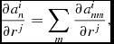 $$\begin{equation}
\frac{\partial a^{i}_{n}}{\partial r^{j}} = \sum _{m} \frac{\partial a^{i}_{nm}}{\partial r^{j}},
\end{equation}$$
$$\begin{equation}
\frac{\partial a^{i}_{n}}{\partial r^{j}} = \sum _{m} \frac{\partial a^{i}_{nm}}{\partial r^{j}},
\end{equation}$$
where
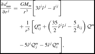 $$\begin{eqnarray}
\frac{\partial a_{nm}^{i}}{\partial r^{j}} &= & \frac{GM_{m}}{r^{3}} \bigg [ 3\hat{r}^{i} \hat{r}^{j} - \delta ^{ij} \bigg ] \nonumber \\
& &+ \,\frac{1}{r^{5}} \left[ Q_{ij}^{m} + \left(\frac{35}{2} \hat{r}^{i} \hat{r}^{j} - \frac{5}{2} \delta _{ij}\right) \mathcal {Q}^{m} \right. \nonumber \\
&& -\, 5 \hat{r}^{i} \mathcal {Q}_{j}^{m} - 5 \hat{r}^{j} \mathcal {Q}_{i}^{m} \bigg ],
\end{eqnarray}$$
$$\begin{eqnarray}
\frac{\partial a_{nm}^{i}}{\partial r^{j}} &= & \frac{GM_{m}}{r^{3}} \bigg [ 3\hat{r}^{i} \hat{r}^{j} - \delta ^{ij} \bigg ] \nonumber \\
& &+ \,\frac{1}{r^{5}} \left[ Q_{ij}^{m} + \left(\frac{35}{2} \hat{r}^{i} \hat{r}^{j} - \frac{5}{2} \delta _{ij}\right) \mathcal {Q}^{m} \right. \nonumber \\
&& -\, 5 \hat{r}^{i} \mathcal {Q}_{j}^{m} - 5 \hat{r}^{j} \mathcal {Q}_{i}^{m} \bigg ],
\end{eqnarray}$$
and ten independent components of the second derivatives, given by
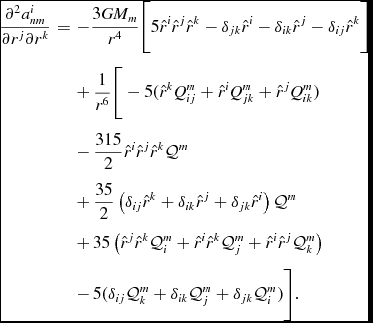 $$\begin{eqnarray}
\frac{\partial ^{2} a^{i}_{nm}}{\partial r^{j} \partial r^{k}} &= & -\frac{3GM_{m}}{r^{4}} \bigg [ 5 \hat{r}^{i} \hat{r}^{j} \hat{r}^{k} - \delta _{jk} \hat{r}^{i} - \delta _{ik} \hat{r}^{j} - \delta _{ij} \hat{r}^{k} \bigg ] \nonumber \\
&& +\, \frac{1}{r^{6}} \bigg [ -5(\hat{r}^{k} Q^{m}_{ij} + \hat{r}^{i} Q^{m}_{jk} + \hat{r}^{j} Q^{m}_{ik}) \nonumber \\
&& -\, \frac{315}{2}\hat{r}^{i}\hat{r}^{j}\hat{r}^{k} \mathcal {Q}^{m} \nonumber \\
&& + \,\frac{35}{2} \left(\delta _{ij} \hat{r}^{k} + \delta _{ik} \hat{r}^{j} + \delta _{jk} \hat{r}^{i} \right) \mathcal {Q}^{m} \nonumber \\
&& +\, 35 \left( \hat{r}^{j} \hat{r}^{k} \mathcal {Q}^{m}_{i} + \hat{r}^{i} \hat{r}^{k} \mathcal {Q}^{m}_{j} + \hat{r}^{i} \hat{r}^{j} \mathcal {Q}^{m}_{k} \right) \nonumber \\
&& -\, 5 (\delta _{ij} \mathcal {Q}^{m}_{k} + \delta _{ik} \mathcal {Q}^{m}_{j} + \delta _{jk} \mathcal {Q}^{m}_{i}) \bigg ].
\end{eqnarray}$$
$$\begin{eqnarray}
\frac{\partial ^{2} a^{i}_{nm}}{\partial r^{j} \partial r^{k}} &= & -\frac{3GM_{m}}{r^{4}} \bigg [ 5 \hat{r}^{i} \hat{r}^{j} \hat{r}^{k} - \delta _{jk} \hat{r}^{i} - \delta _{ik} \hat{r}^{j} - \delta _{ij} \hat{r}^{k} \bigg ] \nonumber \\
&& +\, \frac{1}{r^{6}} \bigg [ -5(\hat{r}^{k} Q^{m}_{ij} + \hat{r}^{i} Q^{m}_{jk} + \hat{r}^{j} Q^{m}_{ik}) \nonumber \\
&& -\, \frac{315}{2}\hat{r}^{i}\hat{r}^{j}\hat{r}^{k} \mathcal {Q}^{m} \nonumber \\
&& + \,\frac{35}{2} \left(\delta _{ij} \hat{r}^{k} + \delta _{ik} \hat{r}^{j} + \delta _{jk} \hat{r}^{i} \right) \mathcal {Q}^{m} \nonumber \\
&& +\, 35 \left( \hat{r}^{j} \hat{r}^{k} \mathcal {Q}^{m}_{i} + \hat{r}^{i} \hat{r}^{k} \mathcal {Q}^{m}_{j} + \hat{r}^{i} \hat{r}^{j} \mathcal {Q}^{m}_{k} \right) \nonumber \\
&& -\, 5 (\delta _{ij} \mathcal {Q}^{m}_{k} + \delta _{ik} \mathcal {Q}^{m}_{j} + \delta _{jk} \mathcal {Q}^{m}_{i}) \bigg ].
\end{eqnarray}$$
The acceleration on each individual particle inside the leaf node n is then computed using a second-order Taylor series expansion of  ${\bm a}_{\rm node}^{n}$ about the node centre, i.e.
 $$\begin{equation}
a^{i}_{{\rm long}, a} = a^{i}_{n} + \Delta x^{j} \frac{\partial a_{n}^{i}}{\partial r^{j}} + \frac{1}{2} \Delta x^{j} \Delta x^{k} \frac{\partial ^{2} a_{n}^{i}}{\partial r^{j}\partial r^{k}},
\end{equation}$$
$$\begin{equation}
a^{i}_{{\rm long}, a} = a^{i}_{n} + \Delta x^{j} \frac{\partial a_{n}^{i}}{\partial r^{j}} + \frac{1}{2} \Delta x^{j} \Delta x^{k} \frac{\partial ^{2} a_{n}^{i}}{\partial r^{j}\partial r^{k}},
\end{equation}$$
where Δxia ≡ xia − xi 0 is the relative distance of each particle from the node centre of mass. Pseudo-code for the resulting force evaluation is shown in Figure A5.
The quadrupole moments are computed during the tree build using
 $$\begin{equation}
Q_{ij} = \sum _{a} m_{a} \left[ 3 \Delta x^{i} \Delta x^{j} - (\Delta x)^{2} \delta ^{ij}\right],
\end{equation}$$
$$\begin{equation}
Q_{ij} = \sum _{a} m_{a} \left[ 3 \Delta x^{i} \Delta x^{j} - (\Delta x)^{2} \delta ^{ij}\right],
\end{equation}$$
where the sum is over all particles in the node. Since Q is a symmetric tensor, only six independent quantities need to be stored (Q xx, Q xy, Q xz, Q yy, Q yz and Q zz).
The current implementation in Phantom is  $\mathcal {O}(N_{\rm {leafnodes}} \log N_{\rm part})$ rather than the $\mathcal {O}(N)$ treecode implementation proposed by Dehnen (Reference Dehnen2000b), since we do not currently implement the symmetric node–node interactions required for $\mathcal {O}(N)$ scaling. Neither does our treecode conserve linear momentum to machine precision, except when θ = 0. Implementing these additional features would be desirable.
2.13. Dust–gas mixtures
Modelling dust–gas mixtures is the first step in the ‘grand challenge’ of protoplanetary disc modelling (Haworth et al. Reference Haworth2016). The public version of Phantom implements dust–gas mixtures using two approaches. One models the dust and gas as two separate types of particles (two-fluid), as presented in Laibe & Price (Reference Laibe and Price2012a, Reference Laibe and Price2012b), and the other, for small grains, using a single type of particle that represents the combination of dust and gas together (one-fluid), as described in Price & Laibe (Reference Price and Laibe2015a). Various combinations of these algorithms have been used in our recent papers using Phantom, including Dipierro et al. (Reference Dipierro, Price, Laibe, Hirsh and Cerioli2015, Reference Dipierro, Laibe, Price and Lodato2016), Ragusa et al. (Reference Ragusa, Dipierro, Lodato, Laibe and Price2017), and Tricco et al. (Reference Tricco, Price and Laibe2017) (see also Hutchison et al. Reference Hutchison, Price, Laibe and Maddison2016).
In the two-fluid implementation, the dust and gas are treated as two separate fluids coupled by a drag term with only explicit timestepping. In the one-fluid implementation, the dust is treated as part of the mixture, with an evolution equation for the dust fraction.
2.13.1. Continuum equations
The two-fluid formulation is based on the continuum equations in the form:
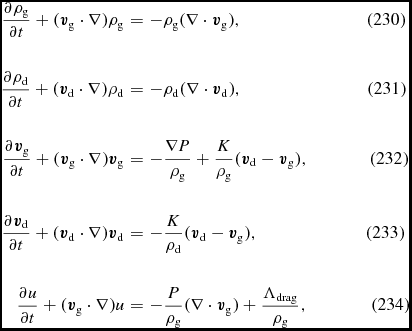 $$\begin{eqnarray*}
\hspace*{30pt}\frac{\partial \rho _{\rm g}}{\partial t} + ({\bm v}_{\rm g}\cdot \nabla ) \rho _{\rm g} &=& -\rho _{\rm g} (\nabla \cdot {\bm v}_{\rm g}),\hspace*{64pt}(230)\\[10pt]
\hspace*{30pt}\frac{\partial \rho _{\rm d}}{\partial t} + ({\bm v}_{\rm d}\cdot \nabla ) \rho _{\rm d} &=& -\rho _{\rm d} (\nabla \cdot {\bm v}_{\rm d}),\hspace*{64pt}(231)\\[10pt]
\hspace*{20pt}\frac{\partial {\bm v}_{\rm g}}{\partial t} + ({\bm v}_{\rm g}\cdot \nabla ) {\bm v}_{\rm g} &=& -\frac{\nabla P}{\rho _{\rm g}} + \frac{K}{\rho _{\rm g}} ({\bm v}_{\rm d}- {\bm v}_{\rm g}),\hspace*{31pt}(232)\\[10pt]
\hspace*{30pt}\frac{\partial {\bm v}_{\rm d}}{\partial t} + ({\bm v}_{\rm d}\cdot \nabla ) {\bm v}_{\rm d} &=& - \frac{K}{\rho _{\rm d}} ({\bm v}_{\rm d}- {\bm v}_{\rm g}),\hspace*{55pt}(233)\\[10pt]
\hspace*{20pt}\frac{\partial u}{\partial t} + ({\bm v}_{\rm g}\cdot \nabla ) u &=& -\frac{P}{\rho _{\rm g}} (\nabla \cdot {\bm v}_{\rm g}) + \frac{\Lambda_{\rm drag}}{\rho_{\rm g}} ,\hspace*{32pt}(234)
\end{eqnarray*}$$
$$\begin{eqnarray*}
\hspace*{30pt}\frac{\partial \rho _{\rm g}}{\partial t} + ({\bm v}_{\rm g}\cdot \nabla ) \rho _{\rm g} &=& -\rho _{\rm g} (\nabla \cdot {\bm v}_{\rm g}),\hspace*{64pt}(230)\\[10pt]
\hspace*{30pt}\frac{\partial \rho _{\rm d}}{\partial t} + ({\bm v}_{\rm d}\cdot \nabla ) \rho _{\rm d} &=& -\rho _{\rm d} (\nabla \cdot {\bm v}_{\rm d}),\hspace*{64pt}(231)\\[10pt]
\hspace*{20pt}\frac{\partial {\bm v}_{\rm g}}{\partial t} + ({\bm v}_{\rm g}\cdot \nabla ) {\bm v}_{\rm g} &=& -\frac{\nabla P}{\rho _{\rm g}} + \frac{K}{\rho _{\rm g}} ({\bm v}_{\rm d}- {\bm v}_{\rm g}),\hspace*{31pt}(232)\\[10pt]
\hspace*{30pt}\frac{\partial {\bm v}_{\rm d}}{\partial t} + ({\bm v}_{\rm d}\cdot \nabla ) {\bm v}_{\rm d} &=& - \frac{K}{\rho _{\rm d}} ({\bm v}_{\rm d}- {\bm v}_{\rm g}),\hspace*{55pt}(233)\\[10pt]
\hspace*{20pt}\frac{\partial u}{\partial t} + ({\bm v}_{\rm g}\cdot \nabla ) u &=& -\frac{P}{\rho _{\rm g}} (\nabla \cdot {\bm v}_{\rm g}) + \frac{\Lambda_{\rm drag}}{\rho_{\rm g}} ,\hspace*{32pt}(234)
\end{eqnarray*}$$
where the subscripts g and d refer to gas and dust properties, K is a drag coefficient and the drag heating is
 $$\begin{equation}
\Lambda _{\rm drag} \equiv K ({\bm v}_{\rm d}- {\bm v}_{\rm g})^{2}.
\end{equation}$$
$$\begin{equation}
\Lambda _{\rm drag} \equiv K ({\bm v}_{\rm d}- {\bm v}_{\rm g})^{2}.
\end{equation}$$
The implementation in Phantom currently neglects any thermal coupling between the dust and the gas (see Laibe & Price Reference Laibe and Price2012a), aside from the drag heating. Thermal effects are important for smaller grains since they control the heating and cooling of the gas (e.g. Dopcke et al. Reference Dopcke, Glover, Clark and Klessen2011). Currently, the internal energy (u) of dust particles is simply set to zero.
2.13.2. Stopping time
The stopping time
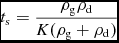 $$\begin{equation}
t_{\rm s} = \frac{\rho _{\rm g} \rho _{\rm d}}{K(\rho _{\rm g} + \rho _{\rm d})}
\end{equation}$$
$$\begin{equation}
t_{\rm s} = \frac{\rho _{\rm g} \rho _{\rm d}}{K(\rho _{\rm g} + \rho _{\rm d})}
\end{equation}$$
is the characteristic timescale for the exponential decay of the differential velocity between the two phases caused by the drag. In the code, t s is by default specified in physical units, which means that code units need to be defined appropriately when simulating dust–gas mixtures.
2.13.3. Two-fluid dust–gas in SPH
In the two-fluid method, the mixture is discretised into two distinct sets of ‘dust’ and ‘gas’ particles. In the following, we adopt the convention from Monaghan & Kocharyan (Reference Monaghan and Kocharyan1995) that subscripts a, b, and c refer to gas particles while i, j, and k refer to dust particles. Hence, (230)–(231) are discretised with a density summation over neighbours of the same type (c.f. Section 2.12.3), giving
 $$\begin{equation}
\rho _{a} = \sum _{b} m_{b} W_{ab} (h_{a}); \hspace{14.22636pt} h_{a} = h_{\rm fact} \left( \frac{m_{a}}{\rho _{a}} \right) ^{1/3},
\end{equation}$$
$$\begin{equation}
\rho _{a} = \sum _{b} m_{b} W_{ab} (h_{a}); \hspace{14.22636pt} h_{a} = h_{\rm fact} \left( \frac{m_{a}}{\rho _{a}} \right) ^{1/3},
\end{equation}$$
for a gas particle, and
 $$\begin{equation}
\rho _{i} = \sum _{j} m_{j} W_{ij} (h_{i}); \hspace{14.22636pt} h_{i} = h_{\rm fact} \left( \frac{m_{i}}{\rho _{i}} \right) ^{1/3},
\end{equation}$$
$$\begin{equation}
\rho _{i} = \sum _{j} m_{j} W_{ij} (h_{i}); \hspace{14.22636pt} h_{i} = h_{\rm fact} \left( \frac{m_{i}}{\rho _{i}} \right) ^{1/3},
\end{equation}$$
for a dust particle. The kernel used for density is the same as usual (Section 2.1.6). We discretise the equations of motion for the gas particles, (232), using
 $$\begin{equation}
\left(\frac{{\rm d}{\bm v}_{a}}{{\rm d}t}\right)_{\rm drag} = -3 \sum _{j} m_{j} \frac{{\bm v}_{aj} \cdot \hat{\bm r}_{aj}}{(\rho _{a} + \rho _{j}) t^{\rm s}_{aj}} \hat{\bm r}_{aj} D_{aj} (h_{a}),
\end{equation}$$
$$\begin{equation}
\left(\frac{{\rm d}{\bm v}_{a}}{{\rm d}t}\right)_{\rm drag} = -3 \sum _{j} m_{j} \frac{{\bm v}_{aj} \cdot \hat{\bm r}_{aj}}{(\rho _{a} + \rho _{j}) t^{\rm s}_{aj}} \hat{\bm r}_{aj} D_{aj} (h_{a}),
\end{equation}$$
and for dust, (233), using
 $$\begin{equation}
\left(\frac{{\rm d}{\bm v}_{i}}{{\rm d}t}\right)_{\rm drag} = -3 \sum _{b} m_{b} \frac{{\bm v}_{ib} \cdot \hat{\bm r}_{ib}}{(\rho _{i} + \rho _{b}) t^{\rm s}_{ib}} \hat{\bm r}_{ib} D_{ib} (h_{b}),
\end{equation}$$
$$\begin{equation}
\left(\frac{{\rm d}{\bm v}_{i}}{{\rm d}t}\right)_{\rm drag} = -3 \sum _{b} m_{b} \frac{{\bm v}_{ib} \cdot \hat{\bm r}_{ib}}{(\rho _{i} + \rho _{b}) t^{\rm s}_{ib}} \hat{\bm r}_{ib} D_{ib} (h_{b}),
\end{equation}$$
where D is a ‘double hump’ kernel, defined in Section 2.13.4. The drag heating term in the energy equation, (234), is discretised using
 $$\begin{equation}
\left( \frac{{\rm d}u}{{\rm d}t} \right)_{\rm drag} = \frac{\Lambda_{\rm drag}}{\rho_{\rm g}} = 3 \sum _{j} m_{j} \frac{({\bm v}_{aj} \cdot \hat{\bm r}_{aj})^{2}}{(\rho _{a} + \rho _{j}) t^{\rm s}_{aj}} D_{aj} (h_{a}).
\end{equation}$$
$$\begin{equation}
\left( \frac{{\rm d}u}{{\rm d}t} \right)_{\rm drag} = \frac{\Lambda_{\rm drag}}{\rho_{\rm g}} = 3 \sum _{j} m_{j} \frac{({\bm v}_{aj} \cdot \hat{\bm r}_{aj})^{2}}{(\rho _{a} + \rho _{j}) t^{\rm s}_{aj}} D_{aj} (h_{a}).
\end{equation}$$
Notice that gas properties are only defined on gas particles and dust properties are defined only on dust particles, greatly simplifying the algorithm. Buoyancy terms caused by dust particles occupying a finite volume (Monaghan & Kocharyan Reference Monaghan and Kocharyan1995; Laibe & Price Reference Laibe and Price2012a) are negligible in astrophysics because typical grain sizes (μm) are negligible compared to simulation scales of ~au or larger.
2.13.4. Drag kernels
Importantly, we use a ‘double-hump’ shaped kernel function D (Fulk & Quinn Reference Fulk and Quinn1996) instead of the usual bell-shaped kernel W when computing the drag terms. Defining D in terms of a dimensionless kernel function as previously (c.f. Section 2.1.5).
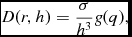 $$\begin{equation}
D(r,h) = \frac{\sigma }{h^{3}} g(q),
\end{equation}$$
$$\begin{equation}
D(r,h) = \frac{\sigma }{h^{3}} g(q),
\end{equation}$$
then the double hump kernels are defined from the usual kernels according to
 $$\begin{equation}
g(q) = q^{2} f(q),
\end{equation}$$
$$\begin{equation}
g(q) = q^{2} f(q),
\end{equation}$$
where the normalisation constant σ is computed by enforcing the usual normalisation condition
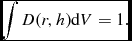 $$\begin{equation}
\int D (r, h) {\rm d}V = 1.
\end{equation}$$
$$\begin{equation}
\int D (r, h) {\rm d}V = 1.
\end{equation}$$
Figure 4 shows the functional forms of the double hump kernels used in Phantom. Using double hump kernels for the drag terms was found by Laibe & Price (Reference Laibe and Price2012a) to give a factor of 10 better accuracy at no additional cost. The key feature is that these kernels are zero at the origin putting more weight in the outer parts of the kernel where the velocity difference is large. This also solves the problem of how to define the unit vector in the drag terms (239)–(241)—it does not matter since D is also zero at the origin.
Double hump smoothing kernels D(r, h) available in Phantom, used in the computation of the dust–gas drag force.
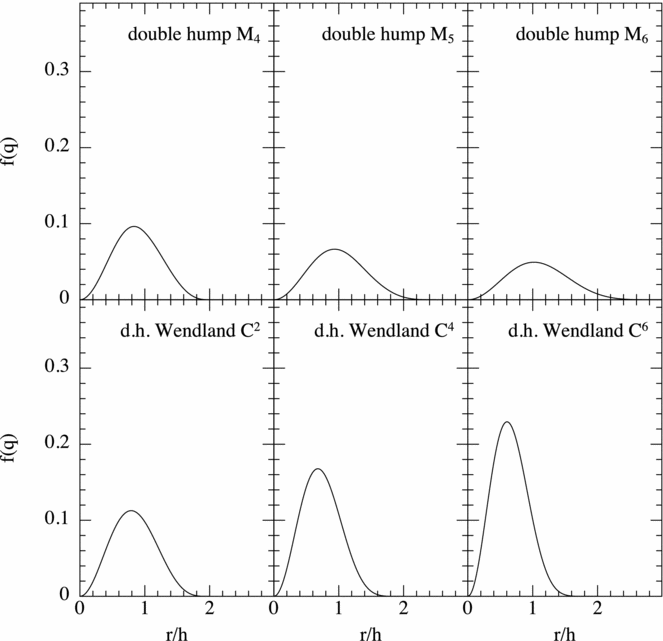
2.13.5. Stopping time in SPH
The stopping time is defined between a pair of particles, using the properties of gas and dust defined on the particle of the respective type, i.e.
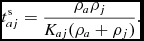 $$\begin{equation}
t^{\rm s}_{aj} = \frac{\rho _{a} \rho _{j}}{K_{aj} (\rho _{a} + \rho _{j})}.
\end{equation}$$
$$\begin{equation}
t^{\rm s}_{aj} = \frac{\rho _{a} \rho _{j}}{K_{aj} (\rho _{a} + \rho _{j})}.
\end{equation}$$
The default prescription for the stopping time in Phantom automatically selects a physical drag regime appropriate to the grain size, as described below and in Laibe & Price (Reference Laibe and Price2012b). Options to use either a constant K or a constant t s between pairs are also implemented, useful for testing and debugging (c.f. Section 5.9).
2.13.6. Epstein drag
To determine the appropriate physical drag regime, we use the procedure suggested by Stepinski & Valageas (Reference Stepinski and Valageas1996) where we first evaluate the Knudsen number
 $$\begin{equation}
K_{\rm n} = \frac{9\lambda _{\rm g}}{4 s_{\rm grain}},
\end{equation}$$
$$\begin{equation}
K_{\rm n} = \frac{9\lambda _{\rm g}}{4 s_{\rm grain}},
\end{equation}$$
where s grain is the grain size and λg is the gas mean free path (see Section 2.13.8, below, for how this is evaluated). For K n ⩾ 1, the drag between a particle pair is computed using the generalised formula for Epstein drag from Kwok (Reference Kwok1975), as described in Paardekooper & Mellema (Reference Paardekooper and Mellema2006) and Laibe & Price (Reference Laibe and Price2012b), giving
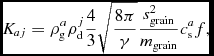 $$\begin{equation}
K_{aj} = \rho ^{a}_{\rm g} \rho ^{j}_{\rm d} \frac{4}{3} \sqrt{\frac{8\pi }{\gamma }} \frac{s_{\rm grain}^{2}}{m_{\rm grain}} c^{a}_{\rm s} f,
\end{equation}$$
$$\begin{equation}
K_{aj} = \rho ^{a}_{\rm g} \rho ^{j}_{\rm d} \frac{4}{3} \sqrt{\frac{8\pi }{\gamma }} \frac{s_{\rm grain}^{2}}{m_{\rm grain}} c^{a}_{\rm s} f,
\end{equation}$$
where
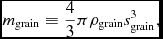 $$\begin{equation}
m_{\rm grain} \equiv \frac{4}{3} \pi \rho _{\rm grain} s_{\rm grain}^{3},
\end{equation}$$
$$\begin{equation}
m_{\rm grain} \equiv \frac{4}{3} \pi \rho _{\rm grain} s_{\rm grain}^{3},
\end{equation}$$
and ρgrain is the intrinsic grain density, which is 3 g/cm3 by default. The variable f is a correction for supersonic drift velocities given by (Kwok Reference Kwok1975)
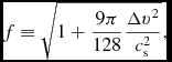 $$\begin{equation}
f \equiv \sqrt{1 + \frac{9\pi }{128} \frac{\Delta v^{2}}{c_{\rm s}^{2}}},
\end{equation}$$
$$\begin{equation}
f \equiv \sqrt{1 + \frac{9\pi }{128} \frac{\Delta v^{2}}{c_{\rm s}^{2}}},
\end{equation}$$
where  $\Delta v \equiv \vert {\bm v}_{\rm d}- {\bm v}_{\rm g}\vert = v_{\rm d}^{j} - v_{\rm g}^{a}$. The stopping time is therefore
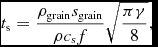 $$\begin{equation}
t_{\rm s} = \frac{ \rho _{\rm grain} s_{\rm grain}}{\rho c_{\rm s}f} \sqrt{\frac{\pi \gamma }{8}},
\end{equation}$$
$$\begin{equation}
t_{\rm s} = \frac{ \rho _{\rm grain} s_{\rm grain}}{\rho c_{\rm s}f} \sqrt{\frac{\pi \gamma }{8}},
\end{equation}$$
where ρ ≡ ρd + ρg. This formula, (250), reduces to the standard expression for the linear Epstein regime in the limit where the drift velocity is small compared to the sound speed (i.e. f → 1). Figure 5 shows the difference between the above simplified prescription and the exact expression for Epstein drag (Epstein Reference Epstein1924; c.f. equations (11) and (38) in Laibe & Price Reference Laibe and Price2012b) as a function of Δv/c s, which is less than 1% everywhere.
Dependence of the drag stopping time t s on differential Mach number, showing the increased drag (decrease in stopping time) as the velocity difference between dust and gas increases. The black line shows the analytic approximation we employ [Equation (250)] which may be compared to the red line showing the exact expression from Epstein (Reference Epstein1924). The difference is less than 1% everywhere.
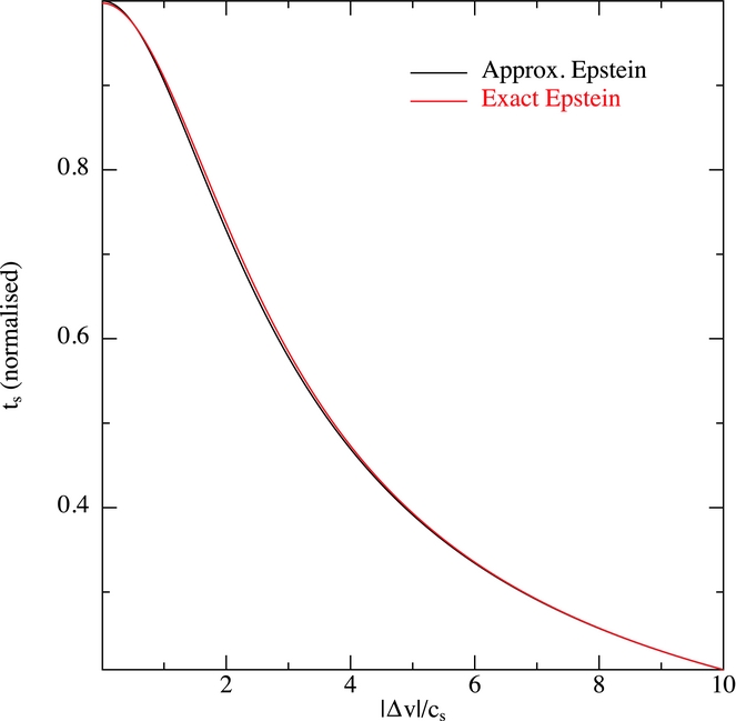
2.13.7. Stokes drag
For K n < 1, we adopt a Stokes drag prescription, describing the drag on a sphere with size larger than the mean free path of the gas (Fan & Zhu Reference Fan and Zhu1998). Here, we use (Laibe & Price Reference Laibe and Price2012b)
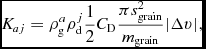 $$\begin{equation}
K_{aj} = \rho ^{a}_{\rm g} \rho ^{j}_{\rm d} \frac{1}{2} C_{\rm D} \frac{\pi s_{\rm grain}^{2}}{m_{\rm grain}} \vert \Delta v\vert ,
\end{equation}$$
$$\begin{equation}
K_{aj} = \rho ^{a}_{\rm g} \rho ^{j}_{\rm d} \frac{1}{2} C_{\rm D} \frac{\pi s_{\rm grain}^{2}}{m_{\rm grain}} \vert \Delta v\vert ,
\end{equation}$$
where the coefficient C D is given by (Fassio & Probstein Reference Fassio and Probstein1970) (see Whipple Reference Whipple and Elvius1972; Weidenschilling Reference Weidenschilling1977)
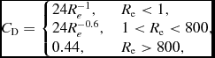 $$\begin{equation}
C_{\rm D} = \left\lbrace \arraycolsep5pt\begin{array}{@{}ll@{}}24 R_{e}^{-1}, & R_{\rm e} < 1, \\
24 R_{e}^{-0.6}, & 1 < R_{\rm e} < 800, \\
0.44, & R_{\rm e} > 800, \end{array}\right.
\end{equation}$$
$$\begin{equation}
C_{\rm D} = \left\lbrace \arraycolsep5pt\begin{array}{@{}ll@{}}24 R_{e}^{-1}, & R_{\rm e} < 1, \\
24 R_{e}^{-0.6}, & 1 < R_{\rm e} < 800, \\
0.44, & R_{\rm e} > 800, \end{array}\right.
\end{equation}$$
where R e is the local Reynolds number around the grain
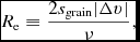 $$\begin{equation}
R_{\rm e} \equiv \frac{2 s_{\rm grain} \vert \Delta v \vert }{\nu },
\end{equation}$$
$$\begin{equation}
R_{\rm e} \equiv \frac{2 s_{\rm grain} \vert \Delta v \vert }{\nu },
\end{equation}$$
and ν is the microscopic viscosity of the gas (see below, not to be confused with the disc viscosity). Similar formulations of Stokes drag can be found elsewhere (see e.g. discussion in Woitke & Helling Reference Woitke and Helling2003 and references therein). The stopping time in the Stokes regime is therefore given by
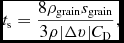 $$\begin{equation}
t_{\rm s} = \frac{8 \rho _{\rm grain} s_{\rm grain}}{3\rho \vert \Delta v\vert C_{\rm D}},
\end{equation}$$
$$\begin{equation}
t_{\rm s} = \frac{8 \rho _{\rm grain} s_{\rm grain}}{3\rho \vert \Delta v\vert C_{\rm D}},
\end{equation}$$
where it remains to evaluate ν and λg.
2.13.8. Kinematic viscosity and mean free path
We evaluate the microscopic kinematic viscosity, ν, assuming gas molecules interact as hard spheres, following Chapman & Cowling (Reference Chapman and Cowling1970). The viscosity is computed from the mean free path and sound speed according to
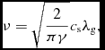 $$\begin{equation}
\nu = \sqrt{\frac{2}{\pi \gamma }} c_{\rm s} \lambda _{\rm g},
\end{equation}$$
$$\begin{equation}
\nu = \sqrt{\frac{2}{\pi \gamma }} c_{\rm s} \lambda _{\rm g},
\end{equation}$$
with the mean free path defined by relating this expression to the expression for the dynamic viscosity of the gas (Chapman & Cowling Reference Chapman and Cowling1970) given by
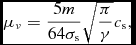 $$\begin{equation}
\mu _{\nu } = \frac{5m}{64\sigma _{\rm s}} \sqrt{\frac{\pi }{\gamma }} c_{\rm s},
\end{equation}$$
$$\begin{equation}
\mu _{\nu } = \frac{5m}{64\sigma _{\rm s}} \sqrt{\frac{\pi }{\gamma }} c_{\rm s},
\end{equation}$$
with μν = ρgν, giving
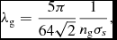 $$\begin{equation}
\lambda _{\rm g} = \frac{5\pi }{64 \sqrt{2}} \frac{1}{n_{\rm g} \sigma _{s}},
\end{equation}$$
$$\begin{equation}
\lambda _{\rm g} = \frac{5\pi }{64 \sqrt{2}} \frac{1}{n_{\rm g} \sigma _{s}},
\end{equation}$$
where n g = ρg/m is the number density of molecules and σs is the collisional cross section. To compute this, Phantom currently assumes the gas is molecular Hydrogen, such that the mass of each molecule and the collisional cross section are given by
 $$\begin{equation}
m = 2 m_{\rm H}, \\
\end{equation}$$
$$\begin{equation}
m = 2 m_{\rm H}, \\
\end{equation}$$
 $$\begin{equation}
\sigma _{\rm s} = 2.367 \times 10^{-15} {\rm cm}^{2}.
\end{equation}$$
$$\begin{equation}
\sigma _{\rm s} = 2.367 \times 10^{-15} {\rm cm}^{2}.
\end{equation}$$
2.13.9. Stokes/Epstein transition
At the transition between the two regimes, assuming R e < 1, (254) reduces to
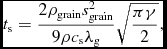 $$\begin{equation}
t_{\rm s} = \frac{2 \rho _{\rm grain} s_{\rm grain}^{2}}{9 \rho c_{\rm s} \lambda _{\rm g}} \sqrt{\frac{\pi \gamma }{2}},
\end{equation}$$
$$\begin{equation}
t_{\rm s} = \frac{2 \rho _{\rm grain} s_{\rm grain}^{2}}{9 \rho c_{\rm s} \lambda _{\rm g}} \sqrt{\frac{\pi \gamma }{2}},
\end{equation}$$
which is the same as the Epstein drag in the subsonic regime when λg = 4s grain/9, i.e. K n = 1. That this transition is indeed continuous in the code is demonstrated in Figure 6, which shows the transition from Epstein to Stokes drag and also through each of the Stokes regimes in (252) by varying the grain size while keeping the other parameters fixed. For simplicity, we assumed a fixed Δv = 0.01c s in this plot, even though in general one would expect Δv to increase with stopping time [see Equation (270)].
Drag stopping time t s (in years) as a function of grain size, showing the continuous transition between the Epstein and Stokes drag regimes. The example shown assumes fixed density ρ = 10−13g/cm3 and sound speed c s = 6 × 104 cm/s with subsonic drag Δv = 0.01c s and material density ρgrain = 3g/cm3.
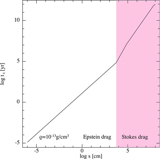
2.13.10. Self-gravity of dust
With self-gravity turned on, dust particles interact in the same way as stars or dark matter (Section 2.12.3), with a softening length equal to the smoothing length determined from the density of neighbouring dust particles. Dust particles can be accreted by sink particles (Section 2.8.2), but a sink cannot currently be created from dust particles (Section 2.8.4). There is currently no mechanism in the code to handle the collapse of dust to form a self-gravitating object independent of the gas.
2.13.11. Timestep constraint
For the two-fluid method, the timestep is constrained by the stopping time according to
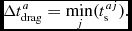 $$\begin{equation}
\Delta t^{a}_{\rm drag} = \min _{j} ( t_{\rm s}^{aj}).
\end{equation}$$
$$\begin{equation}
\Delta t^{a}_{\rm drag} = \min _{j} ( t_{\rm s}^{aj}).
\end{equation}$$
This requirement, alongside the spatial resolution requirement h ≲ c st s (Laibe & Price Reference Laibe and Price2012a), means the two-fluid method becomes both prohibitively slow and increasingly inaccurate for small grains. In this regime, one should switch to the one-fluid method, as described below.
2.13.12. Continuum equations: One-fluid
In Laibe & Price (Reference Laibe and Price2014a), we showed that the two-fluid equations, (230)–(234), can be rewritten as a single fluid mixture using a change of variables given by
 $$\begin{eqnarray}
\rho \equiv \rho _{\rm g} + \rho _{\rm d},
\end{eqnarray}$$
$$\begin{eqnarray}
\rho \equiv \rho _{\rm g} + \rho _{\rm d},
\end{eqnarray}$$
 $$\begin{eqnarray}
\epsilon \equiv \rho _{\rm d}/\rho ,
\end{eqnarray}$$
$$\begin{eqnarray}
\epsilon \equiv \rho _{\rm d}/\rho ,
\end{eqnarray}$$
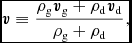 $$\begin{eqnarray}
{\bm v} \equiv \frac{\rho _{\rm g} {\bm v}_{\rm g}+ \rho _{\rm d} {\bm v}_{\rm d}}{ \rho _{\rm g} + \rho _{\rm d} },
\end{eqnarray}$$
$$\begin{eqnarray}
{\bm v} \equiv \frac{\rho _{\rm g} {\bm v}_{\rm g}+ \rho _{\rm d} {\bm v}_{\rm d}}{ \rho _{\rm g} + \rho _{\rm d} },
\end{eqnarray}$$
 $$\begin{eqnarray}
\Delta {\bm v} \equiv {\bm v}_{\rm d}- {\bm v}_{\rm g},
\end{eqnarray}$$
$$\begin{eqnarray}
\Delta {\bm v} \equiv {\bm v}_{\rm d}- {\bm v}_{\rm g},
\end{eqnarray}$$
where ρ is the combined density, ε is the dust fraction,  ${\bm v}$ is the barycentric velocity, and $\Delta {\bm v}$ is the differential velocity between the dust and gas.
In Laibe & Price (Reference Laibe and Price2014a), we derived the full set of evolution equations in these variables, and in Laibe & Price (Reference Laibe and Price2014c), implemented and tested an algorithm to solve these equations in SPH. However, using a fluid approximation cannot properly capture the velocity dispersion of large grains, as occurs for example when large planetesimals stream simultaneously in both directions through the midplane of a protoplanetary disc. For this reason, the one-fluid equations are better suited to treating small grains, where the stopping time is shorter than the computational timestep. In this limit, we employ the ‘terminal velocity approximation’ (e.g. Youdin & Goodman Reference Youdin and Goodman2005) and the evolution equations reduce to (Laibe & Price Reference Laibe and Price2014a; Price & Laibe Reference Price and Laibe2015a)
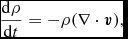 $$\begin{eqnarray}
\frac{{\rm d}\rho }{{\rm d}t} = -\rho (\nabla \cdot {\bm v}),
\end{eqnarray}$$
$$\begin{eqnarray}
\frac{{\rm d}\rho }{{\rm d}t} = -\rho (\nabla \cdot {\bm v}),
\end{eqnarray}$$
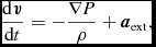 $$\begin{eqnarray}
\frac{{\rm d}{\bm v}}{{\rm d}t} = -\frac{\nabla P}{\rho } + {\bm a}_{\rm ext},
\end{eqnarray}$$
$$\begin{eqnarray}
\frac{{\rm d}{\bm v}}{{\rm d}t} = -\frac{\nabla P}{\rho } + {\bm a}_{\rm ext},
\end{eqnarray}$$
 $$\begin{eqnarray}
\frac{{\rm d}\epsilon }{{\rm d}t} = -\frac{1}{\rho } \nabla \cdot \left[{\epsilon (1 - \epsilon ) \rho \Delta {\bm v}}\right],
\end{eqnarray}$$
$$\begin{eqnarray}
\frac{{\rm d}\epsilon }{{\rm d}t} = -\frac{1}{\rho } \nabla \cdot \left[{\epsilon (1 - \epsilon ) \rho \Delta {\bm v}}\right],
\end{eqnarray}$$
 $$\begin{eqnarray}
\frac{{\rm d}u}{{\rm d}t} = -\frac{P}{\rho } (\nabla \cdot {\bm v}) + \epsilon (\Delta {\bm v} \cdot \nabla ) u,
\end{eqnarray}$$
$$\begin{eqnarray}
\frac{{\rm d}u}{{\rm d}t} = -\frac{P}{\rho } (\nabla \cdot {\bm v}) + \epsilon (\Delta {\bm v} \cdot \nabla ) u,
\end{eqnarray}$$
where
 $$\begin{equation}
\Delta {\bm v} \equiv t_{\rm s} \left({\bm a}_{\rm d} - {\bm a}_{\rm g}\right),
\end{equation}$$
$$\begin{equation}
\Delta {\bm v} \equiv t_{\rm s} \left({\bm a}_{\rm d} - {\bm a}_{\rm g}\right),
\end{equation}$$
where  ${\bm a}_{\rm d}$ and ${\bm a}_{\rm g}$ refers to any acceleration acting only on the dust or gas phase, respectively. For the simple case of pure hydrodynamics, the only difference is the pressure gradient, giving
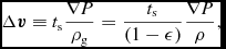 $$\begin{equation}
\Delta {\bm v} \equiv t_{\rm s} \frac{\nabla P}{\rho _{\rm g}} = \frac{t_{\rm s}}{(1 - \epsilon )} \frac{\nabla P}{\rho },
\end{equation}$$
$$\begin{equation}
\Delta {\bm v} \equiv t_{\rm s} \frac{\nabla P}{\rho _{\rm g}} = \frac{t_{\rm s}}{(1 - \epsilon )} \frac{\nabla P}{\rho },
\end{equation}$$
such that (268) becomes
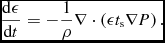 $$\begin{equation}
\frac{{\rm d}\epsilon }{{\rm d}t} = -\frac{1}{\rho } \nabla \cdot \left({\epsilon t_{\rm s}\nabla P}\right).
\end{equation}$$
$$\begin{equation}
\frac{{\rm d}\epsilon }{{\rm d}t} = -\frac{1}{\rho } \nabla \cdot \left({\epsilon t_{\rm s}\nabla P}\right).
\end{equation}$$
Importantly, the one-fluid dust algorithm does not result in any heating term in du/dt due to drag, because this term is  $\mathcal {O}(\Delta {\bm v}^{2})$ and thus negligible (Laibe & Price Reference Laibe and Price2014a).
2.13.13. Visualisation of one-fluid results
Finally, when visualising results of one-fluid calculations, one must reconstruct the properties of the dust and gas in post-processing. We use
 $$\begin{eqnarray}
\rho _{\rm g} = (1 - \epsilon ) \rho ,
\end{eqnarray}$$
$$\begin{eqnarray}
\rho _{\rm g} = (1 - \epsilon ) \rho ,
\end{eqnarray}$$
 $$\begin{eqnarray}
\rho _{\rm d} = \epsilon \rho ,
\end{eqnarray}$$
$$\begin{eqnarray}
\rho _{\rm d} = \epsilon \rho ,
\end{eqnarray}$$
 $$\begin{eqnarray}
{\bm v}_{\rm g} = {\bm v} - \epsilon \Delta {\bm v},
\end{eqnarray}$$
$$\begin{eqnarray}
{\bm v}_{\rm g} = {\bm v} - \epsilon \Delta {\bm v},
\end{eqnarray}$$
 $$\begin{eqnarray}
{\bm v}_{\rm d} = {\bm v} + (1 - \epsilon ) \Delta {\bm v}.
\end{eqnarray}$$
$$\begin{eqnarray}
{\bm v}_{\rm d} = {\bm v} + (1 - \epsilon ) \Delta {\bm v}.
\end{eqnarray}$$
To visualise the one-fluid results in a similar manner to those from the two-fluid method, we reconstruct a set of ‘dust’ and ‘gas’ particles with the same positions but with the respective properties of each type of fluid particle copied onto them. We compute  $\Delta {\bm v}$ from (271) using the pressure gradient computed using (34), multiplied by the stopping time and the gas fraction. See Price & Laibe (Reference Price and Laibe2015a) for more details.
2.13.14. One-fluid dust–gas implementation
Our implementation of the one-fluid method in Phantom follows Price & Laibe (Reference Price and Laibe2015a) with a few minor changes and correctionsFootnote 7. In particular, we use the variable  $s = \sqrt{\epsilon \rho }$ described in Appendix B of Price & Laibe (Reference Price and Laibe2015a) to avoid problems with negative dust fractions. The evolution equation (268) expressed in terms of s is given by
 $$\begin{equation}
\frac{{\rm d}s}{{\rm d}t} = -\frac{1}{2s} \nabla \cdot \left( \frac{\rho _{\rm g} \rho _{\rm d}}{\rho } \Delta {\bm v} \right) - \frac{s}{2} (\nabla \cdot {\bm v}),
\end{equation}$$
$$\begin{equation}
\frac{{\rm d}s}{{\rm d}t} = -\frac{1}{2s} \nabla \cdot \left( \frac{\rho _{\rm g} \rho _{\rm d}}{\rho } \Delta {\bm v} \right) - \frac{s}{2} (\nabla \cdot {\bm v}),
\end{equation}$$
which for the case of hydrodynamics becomes
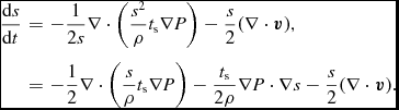 $$\begin{eqnarray}
\frac{{\rm d}s}{{\rm d}t} & =& -\frac{1}{2s} \nabla \cdot \left( \frac{s^{2}}{\rho } t_{\rm s} \nabla P \right) - \frac{s}{2} (\nabla \cdot {\bm v}), \nonumber \\
& =& -\frac{1}{2} \nabla \cdot \left( \frac{s}{\rho } t_{\rm s} \nabla P \right) - \frac{t_{\rm s}}{2\rho } \nabla P \cdot \nabla s - \frac{s}{2} (\nabla \cdot {\bm v}).
\end{eqnarray}$$
$$\begin{eqnarray}
\frac{{\rm d}s}{{\rm d}t} & =& -\frac{1}{2s} \nabla \cdot \left( \frac{s^{2}}{\rho } t_{\rm s} \nabla P \right) - \frac{s}{2} (\nabla \cdot {\bm v}), \nonumber \\
& =& -\frac{1}{2} \nabla \cdot \left( \frac{s}{\rho } t_{\rm s} \nabla P \right) - \frac{t_{\rm s}}{2\rho } \nabla P \cdot \nabla s - \frac{s}{2} (\nabla \cdot {\bm v}).
\end{eqnarray}$$
The SPH discretisation of this equation is implemented in the form
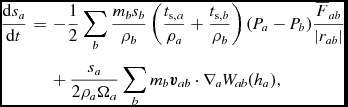 $$\begin{eqnarray}
\frac{{\rm d}s_{a}}{{\rm d}t} &= & - \frac{1}{2} \sum _{b} \frac{m_{b} s_{b}}{\rho _{b}} \left(\frac{t_{{\rm s}, a}}{\rho _{a}} + \frac{t_{{\rm s}, b}}{\rho _b} \right) (P_{a} - P_{b}) \frac{\overline{F}_{ab}}{\vert r_{ab} \vert } \nonumber \\
&& +\, \frac{s_{a}}{2\rho _{a} \Omega _{a}} \sum _{b} m_{b} {\bm v}_{ab} \cdot \nabla _{a} W_{ab} (h_{a}),
\end{eqnarray}$$
$$\begin{eqnarray}
\frac{{\rm d}s_{a}}{{\rm d}t} &= & - \frac{1}{2} \sum _{b} \frac{m_{b} s_{b}}{\rho _{b}} \left(\frac{t_{{\rm s}, a}}{\rho _{a}} + \frac{t_{{\rm s}, b}}{\rho _b} \right) (P_{a} - P_{b}) \frac{\overline{F}_{ab}}{\vert r_{ab} \vert } \nonumber \\
&& +\, \frac{s_{a}}{2\rho _{a} \Omega _{a}} \sum _{b} m_{b} {\bm v}_{ab} \cdot \nabla _{a} W_{ab} (h_{a}),
\end{eqnarray}$$
where  $\overline{F}_{ab} \equiv \frac{1}{2} [ F_{ab} (h_{a}) + F_{ab}(h_{b}) ]$. The thermal energy equation, (269), takes the form
 $$\begin{equation}
\frac{{\rm d}u}{{\rm d}t} = - \frac{P}{\rho } (\nabla \cdot {\bm v}) + \frac{s^{2} t_{\rm s}}{\rho \rho _{\rm g}}\nabla P \cdot \nabla u,
\end{equation}$$
$$\begin{equation}
\frac{{\rm d}u}{{\rm d}t} = - \frac{P}{\rho } (\nabla \cdot {\bm v}) + \frac{s^{2} t_{\rm s}}{\rho \rho _{\rm g}}\nabla P \cdot \nabla u,
\end{equation}$$
the first term of which is identical to (35) and the second term of which is discretised in Phantom according to
 $$\begin{equation}
-\frac{\rho _{a}}{2\rho ^{\rm g}_{a}} \sum _{b} m_{b}\frac{s_{a} s_{b}}{\rho _{a}\rho _{b}} \left(\frac{t_{{\rm s}, a}}{\rho _{a}} + \frac{t_{{\rm s}, b}}{\rho _b} \right) (P_{a} - P_{b}) (u_{a} - u_{b})\frac{\overline{F}_{ab}}{\vert r_{ab} \vert } .
\end{equation}$$
$$\begin{equation}
-\frac{\rho _{a}}{2\rho ^{\rm g}_{a}} \sum _{b} m_{b}\frac{s_{a} s_{b}}{\rho _{a}\rho _{b}} \left(\frac{t_{{\rm s}, a}}{\rho _{a}} + \frac{t_{{\rm s}, b}}{\rho _b} \right) (P_{a} - P_{b}) (u_{a} - u_{b})\frac{\overline{F}_{ab}}{\vert r_{ab} \vert } .
\end{equation}$$
2.13.15. Conservation of dust mass
Conservation of dust mass with the one-fluid scheme is in principle exact because (Price & Laibe Reference Price and Laibe2015a)
 $$\begin{equation}
\frac{{\rm d}}{{\rm d}t} \left( \sum _{a} \frac{m_{a}}{\rho _{a}} s_{a}^{2}\right) = \sum _{a} m_{a} \left( \frac{2s_{a}}{\rho _{a}} \frac{{\rm d}s_{a}}{{\rm d}t} - \frac{s_{a}^{2}}{\rho _{a}^{2}} \frac{{\rm d}\rho _{a}}{{\rm d}t}\right) = 0.
\end{equation}$$
$$\begin{equation}
\frac{{\rm d}}{{\rm d}t} \left( \sum _{a} \frac{m_{a}}{\rho _{a}} s_{a}^{2}\right) = \sum _{a} m_{a} \left( \frac{2s_{a}}{\rho _{a}} \frac{{\rm d}s_{a}}{{\rm d}t} - \frac{s_{a}^{2}}{\rho _{a}^{2}} \frac{{\rm d}\rho _{a}}{{\rm d}t}\right) = 0.
\end{equation}$$
In practice, some violation of this can occur because although the above algorithm guarantees positivity of the dust fraction, it does not guarantee that ε remains less than unity. Under this circumstance, which occurs only rarely, we set ε = max(ε, 1) in the code. However, this violates the conservation of dust mass. This specific issue has been recently addressed in detail in the study by Ballabio et al. (Reference Ballabio, Dipierro, Veronesi, Lodato, Hutchison, Laibe and Price2018). Therefore, in the latest code, there are two main changes as follows:
• Rather than evolve
$s = \sqrt{\epsilon \rho }$, in the most recent code, we instead evolve a new variable $s^{\prime } = \sqrt{\rho _{\rm d}/\rho _{\rm g}}$. This prevents the possibility of ε > 1.• We limit the stopping time such that the timestep from the one fluid algorithm does not severely restrict the computational performance.

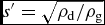
For details of these changes, we refer the reader to Ballabio et al. (Reference Ballabio, Dipierro, Veronesi, Lodato, Hutchison, Laibe and Price2018).
2.13.16. Conservation of energy and momentum
Total energy with the one-fluid scheme can be expressed via
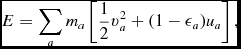 $$\begin{equation}
E =\sum _{a} m_{a} \left[ \frac{1}{2} v^{2}_{a} + (1 - \epsilon _{a}) u_{a} \right],
\end{equation}$$
$$\begin{equation}
E =\sum _{a} m_{a} \left[ \frac{1}{2} v^{2}_{a} + (1 - \epsilon _{a}) u_{a} \right],
\end{equation}$$
which is conserved exactly by the discretisation since
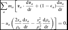 $$\begin{eqnarray}
&&\sum _{a} m_{a} \left[ {\bm v}_{a}\cdot \frac{{\rm d} {\bm v}_{a}}{{\rm d}t} + (1 - \epsilon _{a}) \frac{{\rm d}u_{a}}{{\rm d}t} \right. \nonumber \\
&&\left. -\, u_{a} \left(\frac{2s_{a}}{\rho _{a}}\frac{{\rm d}s_{a}}{{\rm d}t} - \frac{s^{2}_{a}}{\rho _{a}^{2}} \frac{{\rm d}\rho _{a}}{{\rm d}t}\right)\right] = 0.
\end{eqnarray}$$
$$\begin{eqnarray}
&&\sum _{a} m_{a} \left[ {\bm v}_{a}\cdot \frac{{\rm d} {\bm v}_{a}}{{\rm d}t} + (1 - \epsilon _{a}) \frac{{\rm d}u_{a}}{{\rm d}t} \right. \nonumber \\
&&\left. -\, u_{a} \left(\frac{2s_{a}}{\rho _{a}}\frac{{\rm d}s_{a}}{{\rm d}t} - \frac{s^{2}_{a}}{\rho _{a}^{2}} \frac{{\rm d}\rho _{a}}{{\rm d}t}\right)\right] = 0.
\end{eqnarray}$$
Conservation of linear and angular momentum also hold since the discretisation of the momentum equation is identical to the hydrodynamics algorithm.
2.13.17. Timestep constraint
For the one-fluid method, the timestep is constrained by the inverse of the stopping time according to
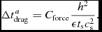 $$\begin{equation}
\Delta t^{a}_{\rm drag} = C_{\rm force} \frac{h^{2}}{ \epsilon t_{\rm s} c_{\rm s}^{2}}.
\end{equation}$$
$$\begin{equation}
\Delta t^{a}_{\rm drag} = C_{\rm force} \frac{h^{2}}{ \epsilon t_{\rm s} c_{\rm s}^{2}}.
\end{equation}$$
This becomes prohibitive precisely in the regime where the one-fluid method is no longer applicable (t s > t Cour; see Laibe & Price Reference Laibe and Price2014a), in which case one should switch to the two-fluid method instead. There is currently no mechanism to automatically switch regimes, though this is possible in principle and may be implemented in a future code version.
2.14. Interstellar medium (ISM) physics
2.14.1. Cooling function
The cooling function in Phantom is based on a set of Fortran modules written by Glover & Mac Low (Reference Glover and Mac Low2007), updated further by Glover et al. (Reference Glover, Federrath, Mac Low and Klessen2010). It includes cooling from atomic lines (H I), molecular excitation (H2), fine structure metal lines (Si I, Si II, O I, C I, and C II), gas–dust collisions, and polycyclic aromatic hydrocarbon (PAH) recombination (see Glover & Mac Low Reference Glover and Mac Low2007 for references on each process). Heating is provided by cosmic rays and the photoelectric effect. The strength of the cooling is a function of the temperature, density, and various chemical abundances. Table 2 summarises these various heating and cooling processes. Figure 7 shows the resulting emissivity ΛE(T) for temperatures between 104 and 108 K. The cooling rate per unit volume is related to the emissivity according to
 $$\begin{equation}
\Lambda _{\rm cool} \equiv n^2 \Lambda _{\rm E} (T) \, {\rm erg} \phantom{s}{\rm s}^{-1} {\rm cm}^{-3},
\end{equation}$$
$$\begin{equation}
\Lambda _{\rm cool} \equiv n^2 \Lambda _{\rm E} (T) \, {\rm erg} \phantom{s}{\rm s}^{-1} {\rm cm}^{-3},
\end{equation}$$
where n is the number density. The cooling in the energy equation corresponds to
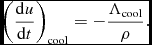 $$\begin{equation}
\left(\frac{{\rm d}u}{{\rm d}t}\right)_{\rm cool} = -\frac{\Lambda _{\rm cool}}{\rho }.
\end{equation}$$
$$\begin{equation}
\left(\frac{{\rm d}u}{{\rm d}t}\right)_{\rm cool} = -\frac{\Lambda _{\rm cool}}{\rho }.
\end{equation}$$
These routines were originally adapted for use in sphng (Dobbs et al. Reference Dobbs, Glover, Clark and Klessen2008) and result in an approximate two-phase ISM with temperatures of 100 K and 10 000 K. Note that the cooling depends on a range of parameters (dust-to-gas ratio, cosmic ray ionisation rate, etc.), many of which can be specified at runtime. Table 3 lists the default abundances, which are set to values appropriate for the Warm Neutral Medium taken from Sembach et al. (Reference Sembach, Howk, Ryans and Keenan2000). The abundances listed in Table 3, along with the dust-to-gas ratio, are the only metallicity-dependent parameters that can be changed at runtime. An option for cooling appropriate to the zero metallicity early universe is also available.
Emissivity, ΛE (erg s−1 cm3) as a function of temperature for the ISM cooling assuming default abundances appropriate for the warm neutral medium (WNM). Note that as we treat cooling from atomic hydrogen using a full non-equilibrium treatment, the behaviour of ΛE close to 104 K is highly sensitive to the electron fraction, which in the case shown here is much smaller than it would be in collisional ionisation equilibrium. Values of ΛE below 104 K depend strongly on the current chemical state of the gas and are not shown in this plot.
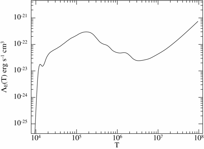
Heating and cooling processes in the Phantom cooling module.
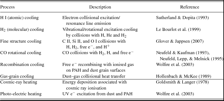
Default fractional abundances for C, O, Si, and e − in the ISM cooling and chemistry modules. Abundances are taken from Sembach et al. (Reference Sembach, Howk, Ryans and Keenan2000) appropriate for the warm neutral medium (WNM). These are lower than solar because it is assumed some fraction of the metals are locked up in dust rather than being available in the gas phase.
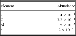
2.14.2. Timestep constraint from cooling
When cooling is used, we apply an additional timestep constraint in the form
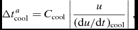 $$\begin{equation}
\Delta t _{\rm cool}^a = C_{\rm cool} \left| \frac{u}{({\rm d}u/{\rm d}t)_{\rm cool}} \right|,
\end{equation}$$
$$\begin{equation}
\Delta t _{\rm cool}^a = C_{\rm cool} \left| \frac{u}{({\rm d}u/{\rm d}t)_{\rm cool}} \right|,
\end{equation}$$
where C cool = 0.3 following Glover & Mac Low (Reference Glover and Mac Low2007). The motivation for this additional constraint is to not allow the cooling to completely decouple from the other equations in the code (Suttner et al. Reference Suttner, Smith, Yorke and Zinnecker1997), and to avoid cooling instabilities that may be generated by numerical errors (Ziegler, Yorke, & Kaisig Reference Ziegler, Yorke and Kaisig1996).
Cooling is currently implemented only with explicit timestepping of (287), where u is evolved alongside velocity in our leapfrog timestepping scheme. However, the substepping scheme described below for the chemical network (Section 2.14.4) is also used to update the cooling on the chemical timestep, meaning that the cooling can evolve on a much shorter timestep than the hydrodynamics when it is used in combination with chemistry, which it is by default. Implementation of an implicit cooling method, namely the one proposed by Townsend (Reference Townsend2009), is under development.
2.14.3. Chemical network
A basic chemical network is included for ISM gas that evolves the abundances of H, H+, e−, and the molecules H2 and CO. The number density of each species, n X, is evolved using simple rate equations of the form
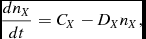 $$\begin{equation}
\frac{dn_X}{dt} = C_X - D_X n_X,
\end{equation}$$
$$\begin{equation}
\frac{dn_X}{dt} = C_X - D_X n_X,
\end{equation}$$
where C X and D X are creation and destruction coefficients for each species. In general, C X and D X are functions of density, temperature, and abundances of other species. The number density of each species, X, is time integrated according to
 $$\begin{equation}
n_X(t+\Delta t) = n_X(t) + \frac{dn_X}{dt} \Delta t.
\end{equation}$$
$$\begin{equation}
n_X(t+\Delta t) = n_X(t) + \frac{dn_X}{dt} \Delta t.
\end{equation}$$
There are in effect only three species to evolve (H, H2, and CO), as the H+ and e− abundances are directly related to the H abundance.
The chemistry of atomic hydrogen is effectively the same as in Glover & Mac Low (Reference Glover and Mac Low2007). H is created by recombination in the gas phase and on grain surfaces, and destroyed by cosmic ray ionisation and free electron collisional ionisation. H2 chemistry is based on the model of Bergin et al. (Reference Bergin, Hartmann, Raymond and Ballesteros-Paredes2004), with H2 created on grain surfaces and destroyed by photo-dissociation and cosmic rays (see Dobbs et al. Reference Dobbs, Glover, Clark and Klessen2008 for computational details).
The underlying processes behind CO chemistry are more complicated, and involve many intermediate species in creating CO from C and O by interactions with H species. Instead of following every intermediate step, we use the model of Nelson & Langer (Reference Nelson and Langer1997) (see Pettitt et al. Reference Pettitt, Dobbs, Acreman and Price2014 for computational details). CO is formed by a gas phase reaction from an intermediate CHZ step after an initial reaction of C+ and H2 (where Z encompasses many similar type species). CO and CHZ are subject to independent photo-destruction, which far outweighs the destruction by cosmic rays. Abundances of C+ and O are used in the CO chemistry, and their abundance is simply the initial value excluding what has been used up in CO formation. Glover & Clark (Reference Glover and Clark2012) test this and a range of simpler and more complicated models, and show that the model adopted here is sufficient for large-scale simulations of CO formation, although it tends to over-produce CO compared to more sophisticated models.
The details for each reaction in the H, H2, and CO chemistry are given in Table 4, with relevant references for each process.
Processes and references for the Phantom ISM chemistry module tracing the evolution of H, H2, and CO.
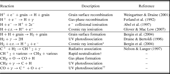
* H + 2 ions produced by cosmic ray ionisation of H2 are assumed to dissociatively recombine to H + H, so that the effective reaction in the code is actually H2 + c.r. → H + H.
† Process is intermediate and is assumed rather than fully represented.
†† C is not present in our chemistry, but is assumed to rapidly photoionise to C+.
2.14.4. Timestep constraint from chemistry
H chemistry is evolved on the cooling timestep, since the timescale on which the H+ abundance changes significantly is generally comparable to or longer than the cooling time. This is not true for H2 and CO. Instead, these species are evolved using a chemical timestepping criterion, where (290) is subcycled during the main time step at the interval Δt chem. If the abundance is decreasing, then the chemical timestep is
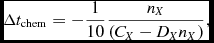 $$\begin{equation}
\Delta t_{\rm chem} = -\frac{1}{10} \frac{n_X}{(C_X - D_X n_X)},
\end{equation}$$
$$\begin{equation}
\Delta t_{\rm chem} = -\frac{1}{10} \frac{n_X}{(C_X - D_X n_X)},
\end{equation}$$
i.e., 10% of the time needed to completely deplete the species. If the abundance is increasing,
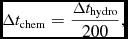 $$\begin{equation}
\Delta t_{\rm chem} = \frac{\Delta t_{\rm hydro}}{200} ,
\end{equation}$$
$$\begin{equation}
\Delta t_{\rm chem} = \frac{\Delta t_{\rm hydro}}{200} ,
\end{equation}$$
where Δt hydro is the timestep size for the hydrodynamics, and was found to be an appropriate value by test simulations. These updated abundances feed directly into the relevant cooling functions. Although the cooling function includes Si I and C I, the abundances of these elements are set to zero in the current chemical model.
2.15. Particle injection
We implement several algorithms for modelling inflow boundary conditions (see Toupin et al. Reference Toupin, Braun, Siess, Jorissen, Gail and Price2015a, Reference Toupin, Braun, Siess, Jorissen, Price, Kerschbaum, Wing and Hron2015b for recent applications) This includes injecting SPH particles in spherical winds from sink particles (both steady and time dependent), in a steady Cartesian flow and for injection at the L 1 point between a pair of sink particles to simulate the formation of accretion discs by Roche Lobe overflow in binary systems.
3 INITIAL CONDITIONS
3.1. Uniform distributions
The simplest method for initialising the particles is to set them on a uniform Cartesian distribution. The lattice arrangement can be cubic (equal particle spacing in each direction, Δx = Δy = Δz), close-packed ( $\Delta y = \sqrt{3/4}\Delta x$, $\Delta z = \sqrt{6}/3 \Delta x$, repeated every three layers in z), hexagonal close-packed (as for close-packed but repeated every two layers in z), or uniform random. The close-packed arrangements are the closest to a ‘relaxed’ particle distribution, but require care with periodic boundary conditions due to the aspect ratio of the lattice. The cubic lattice is not a relaxed arrangement for the particles, but is convenient and sufficient for problems where the initial conditions are quickly erased (e.g. driven turbulence). For problems where initial conditions matter, it is usually best to relax the particle distribution by evolving the simulation for a period of time with a damping term (Section 3.6). This is the approach used, for example, in setting up stars in hydrostatic equilibrium (Section 3.4).
3.2. Stretch mapping
General non-uniform density profiles may be set up using ‘stretch mapping’ (Herant Reference Herant1994). The procedure for spherical distributions is the most commonly used (e.g. Fryer, Hungerford, & Rockefeller Reference Fryer, Hungerford and Rockefeller2007; Rosswog & Price Reference Rosswog and Price2007; Rosswog, Ramirez-Ruiz, & Hix Reference Rosswog, Ramirez-Ruiz and Hix2009), but we have generalised the method for any density profile that is along one coordinate direction (e.g. Price & Monaghan Reference Price and Monaghan2004b). Starting with particles placed in a uniform distribution, the key is that a particle should keep the same relative position in the mass distribution. For each particle with initial coordinate x 0 in the relevant coordinate system, we solve the equation
 $$\begin{equation}
f(x) = \frac{M(x)}{M(x_{\rm max})} - \frac{x_{0} - x_{\rm min}}{(x_{\rm max} - x_{\rm min})} = 0,
\end{equation}$$
$$\begin{equation}
f(x) = \frac{M(x)}{M(x_{\rm max})} - \frac{x_{0} - x_{\rm min}}{(x_{\rm max} - x_{\rm min})} = 0,
\end{equation}$$
where M(x) is the desired density profile integrated along the relevant coordinate direction, i.e.
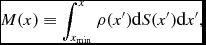 $$\begin{equation}
M(x) \equiv \int _{x_{\rm min}}^{x} \rho (x^{\prime }) \text{d}S(x^{\prime }) \text{d}x^{\prime },
\end{equation}$$
$$\begin{equation}
M(x) \equiv \int _{x_{\rm min}}^{x} \rho (x^{\prime }) \text{d}S(x^{\prime }) \text{d}x^{\prime },
\end{equation}$$
where the area element dS(x′) depends on the geometry and the chosen direction, given by
 $$\begin{equation}
dS(x) = \left\lbrace \arraycolsep5pt\begin{array}{ll}1 & \textrm {Cartesian or cyl./sph. along}\ \phi , \theta \ \text{or}\ z, \\
2\pi x & \textrm {cylindrical along r}, \\
4\pi x^{2} & \textrm {spherical along r}. \end{array}\right.
\end{equation}$$
$$\begin{equation}
dS(x) = \left\lbrace \arraycolsep5pt\begin{array}{ll}1 & \textrm {Cartesian or cyl./sph. along}\ \phi , \theta \ \text{or}\ z, \\
2\pi x & \textrm {cylindrical along r}, \\
4\pi x^{2} & \textrm {spherical along r}. \end{array}\right.
\end{equation}$$
We solve (293) for each particle using Newton–Raphson iterations
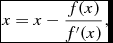 $$\begin{equation}
x = x - \frac{f(x)}{f^{\prime }(x)},
\end{equation}$$
$$\begin{equation}
x = x - \frac{f(x)}{f^{\prime }(x)},
\end{equation}$$
where
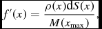 $$\begin{equation}
f^{\prime }(x) = \frac{\rho (x)\text{d}S(x)}{M(x_{\rm max})},
\end{equation}$$
$$\begin{equation}
f^{\prime }(x) = \frac{\rho (x)\text{d}S(x)}{M(x_{\rm max})},
\end{equation}$$
iterating until |f(x)| < 10−9. The Newton–Raphson iterations have second-order convergence, but may fail in extreme cases. Therefore, if the root finding has failed to converge after 30 iterations, we revert to a bisection method, which is only first-order but guaranteed to converge.
Stretch mapping is implemented in such a way that only the desired density function need be specified, either as through an analytic expression (implemented as a function call) or as a tabulated dataset. Since the mass integral in (294) may not be known analytically, we compute this numerically by integrating the density function using the trapezoidal rule.
The disadvantage of stretch mapping is that in spherical or cylindrical geometry it produces defects in the particle distribution arising from the initial Cartesian distribution of the particles. In this case, the particle distribution should be relaxed into a more isotropic equilibrium state before starting the simulation. For stars, for example, this may be done by simulating the star in isolation with artificial damping added (Section 3.6). Alternative approaches are to relax the simulation using an external potential chosen to produce the desired density profile in equilibrium (e.g. Zurek & Benz Reference Zurek and Benz1986; Nagasawa, Nakamura, & Miyama Reference Nagasawa, Nakamura and Miyama1988) or to iteratively ‘cool’ the particle distribution to generate ‘optimal’ initial conditions (Diehl et al. Reference Diehl, Rockefeller, Fryer, Riethmiller and Statler2015).
3.3. Accretion discs
3.3.1. Density field
The accretion disc setup module uses a Monte Carlo particle placement (details in Section A.7) in cylindrical geometry to construct density profiles of the form
 $$\begin{equation}
\rho (x,y,z) = \Sigma _{0} f_{\rm s} \left(\frac{R}{R_{\rm in}}\right)^{-p} \exp {\left(\frac{-z^{2}}{2H^{2}}\right)} ,
\end{equation}$$
$$\begin{equation}
\rho (x,y,z) = \Sigma _{0} f_{\rm s} \left(\frac{R}{R_{\rm in}}\right)^{-p} \exp {\left(\frac{-z^{2}}{2H^{2}}\right)} ,
\end{equation}$$
where Σ0 is the surface density at R = R in (if f s = 1), H ≡ c s/Ω is the scale height (with 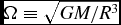 $\Omega \equiv \sqrt{GM/R^{3}}$), p is the power-law index (where p = 3/2 by default following Lodato & Pringle Reference Lodato and Pringle2007), and $f_{\rm s} \equiv (1 - \sqrt{R_{\rm in}/R} )$ is an optional factor to smooth the surface density near the inner disc edge.
Several authors have argued that a more uniform particle placement is preferable for setting up discs in SPH (Cartwright, Stamatellos, & Whitworth Reference Cartwright, Stamatellos and Whitworth2009; Vanaverbeke et al. Reference Vanaverbeke, Keppens, Poedts and Boffin2009). This may be important if one is interested in transient phenomena at the start of a simulation, but otherwise the particle distribution settles to a smooth density distribution within a few orbits (c.f. Lodato & Price Reference Lodato and Price2010).
3.3.2. Velocity field
The orbital velocities of particles in the disc are set by solving the equation for centrifugal equilibrium, i.e.
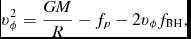 $$\begin{equation}
v_{\phi }^{2} = \frac{GM}{R} - f_{p} - 2v_{\phi } f_{\rm BH},
\end{equation}$$
$$\begin{equation}
v_{\phi }^{2} = \frac{GM}{R} - f_{p} - 2v_{\phi } f_{\rm BH},
\end{equation}$$
where the correction from radial pressure gradients is given by
 $$\begin{equation}
f_{p} = -c_{\rm s}^{2}(R) \left(\frac{3}{2} + p + q + \frac{1}{2f_{\rm s}}\right),
\end{equation}$$
$$\begin{equation}
f_{p} = -c_{\rm s}^{2}(R) \left(\frac{3}{2} + p + q + \frac{1}{2f_{\rm s}}\right),
\end{equation}$$
where q is the index of the sound speed profile such that c s(R) = c s, in(R/R in)−q and f BH is a correction used for discs around a spinning black hole (Nealon et al. Reference Nealon, Price and Nixon2015)
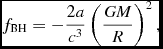 $$\begin{equation}
f_{\rm BH} = - \frac{2a}{c^{3}} \left(\frac{GM}{R}\right)^{2},
\end{equation}$$
$$\begin{equation}
f_{\rm BH} = - \frac{2a}{c^{3}} \left(\frac{GM}{R}\right)^{2},
\end{equation}$$
where a is the black hole spin parameter. The latter assumes Lense–Thirring precession is implemented as in Section 2.4.5. Where self-gravity is used, M is the enclosed mass at a given radius M( < R), otherwise it is simply the mass of the central object. Using the enclosed mass for the self-gravitating case is an approximation since the disc is not spherically symmetric, but the difference is small and the disc relaxes quickly into the true equilibrium. Equation (299) is a quadratic for v ϕ which we solve analytically.
3.3.3. Warps
Warps are applied to the disc (e.g. Lodato & Price Reference Lodato and Price2010; Nealon et al. Reference Nealon, Price and Nixon2015) by rotating the particles about the y-axis by the inclination angle i [in general, a function of radius i ≡ i(R)], according to
 $$\begin{equation}
x^{\prime } = x\cos (i) + z\sin (i), \\
\end{equation}$$
$$\begin{equation}
x^{\prime } = x\cos (i) + z\sin (i), \\
\end{equation}$$
 $$\begin{equation}
y^{\prime } = y, \\
\end{equation}$$
$$\begin{equation}
y^{\prime } = y, \\
\end{equation}$$
 $$\begin{equation}
z^{\prime } = -x\sin (i) + z\cos (i),
\end{equation}$$
$$\begin{equation}
z^{\prime } = -x\sin (i) + z\cos (i),
\end{equation}$$
 $$\begin{equation}
v^{\prime }_{x} = v_{x}\cos (i) + v_{z}\sin (i), \\
\end{equation}$$
$$\begin{equation}
v^{\prime }_{x} = v_{x}\cos (i) + v_{z}\sin (i), \\
\end{equation}$$
 $$\begin{equation}
v^{\prime }_{y} = v_{y}, \\
\end{equation}$$
$$\begin{equation}
v^{\prime }_{y} = v_{y}, \\
\end{equation}$$
 $$\begin{equation}
v^{\prime }_{z} = -v_{x}\sin (i) + v_{z} \cos (i).
\end{equation}$$
$$\begin{equation}
v^{\prime }_{z} = -v_{x}\sin (i) + v_{z} \cos (i).
\end{equation}$$
3.3.4. Setting an α-disc viscosity
The simplest approach to mimicking an α-disc viscosity in SPH is to employ a modified shock viscosity term, setting the desired αSS according to (124) as described in more detail in Section 2.6.1. Since the factor 〈h〉/H is dependent both on resolution and temperature profile (i.e. the q-index), it is computed in the initial setup by taking the desired αSS as input in order to give the required αAV. Although this does not guarantee that αSS is constant with radius and time (this is only true with specific choices of p and q and if the disc is approximately steady), it provides a simple way to prescribe the disc viscosity.
3.4. Stars and binary stars
We implement a general method for setting up ‘realistic’ stellar density profiles, based on either analytic functions (e.g. polytropes) or tabulated data files output from stellar evolution codes [see Iaconi et al. (Reference Iaconi, Reichardt, Staff, De Marco, Passy, Price, Wurster and Herwig2017) for a recent application of this to common envelope evolution].
The basic idea is to set up a uniform density sphere of particles and set the density profile by stretch mapping (see above). The thermal energy of the particles is set so that the pressure gradient is in hydrostatic equilibrium with the self-gravity of the star for the chosen EOS. We then relax the star into equilibrium for several dynamical times using a damping parameter (Section 3.6), before re-launching the simulation with the star on an appropriate orbit.
For simulating red giants, it is preferable to replace the core of the star by a sink particle (see Passy et al. Reference Passy2012; Iaconi et al. Reference Iaconi, Reichardt, Staff, De Marco, Passy, Price, Wurster and Herwig2017). When doing so, one should set the accretion radius of the sink to zero and set a softening length for the sink particle consistent with the original core radius (see Section 2.8.1).
3.5. Galactic initial conditions
In addition to simulating ISM gas in galactic discs with analytic stellar potentials, one may represent bulge-halo-disc components by collisionless N-body particles (see Section 2.12.3). To replace a potential with a resolved system requires care with the initial conditions (i.e. position, velocity, and mass). If setup incorrectly the system will experience radial oscillations and undulations in the rotation curve, which will have strong adverse effects on the gas embedded within. We include algorithms for initialising the static-halo models of Pettitt et al. (Reference Pettitt, Dobbs, Acreman and Bate2015) (which used the sphng SPH code). These initial conditions require the NFW profile to be active and care must be taken to ensure the mass and scale lengths correspond to the rotation curve used to generate the initial conditions. Other codes may alternatively be used to seed multi-component N-body disc galaxies (e.g. Kuijken & Dubinski Reference Kuijken and Dubinski1995a; Boily, Kroupa, & Peñarrubia-Garrido Reference Boily, Kroupa and Peñarrubia-Garrido2001; McMillan & Dehnen Reference McMillan and Dehnen2007; Yurin & Springel Reference Yurin and Springel2014), including magalie (Boily et al. Reference Boily, Kroupa and Peñarrubia-Garrido2001) and galic (Yurin & Springel Reference Yurin and Springel2014) for which we have implemented format readers.
The gas in galactic scale simulations can be setup either in a uniform surface density disc, or according to the Milky Way’s specific surface density. The latter is based on the radial functions given in Wolfire et al. (Reference Wolfire, Hollenbach, McKee, Tielens and Bakes1995). As of yet, we have not implemented a routine for enforcing hydrostatic equilibrium (Springel, Di Matteo, & Hernquist Reference Springel, Di Matteo and Hernquist2005; Wang et al. Reference Wang, Klessen, Dullemond, van den Bosch and Fuchs2010), this may be included in a future update.
3.6. Damping
To relax a particle distribution into equilibrium, we adopt the standard approach (e.g. Gingold & Monaghan Reference Gingold and Monaghan1977) of adding an external acceleration in the form
 $$\begin{equation}
{\bm a}_{\rm ext, damp}^{a} = - f_{\rm d} {\bm v},
\end{equation}$$
$$\begin{equation}
{\bm a}_{\rm ext, damp}^{a} = - f_{\rm d} {\bm v},
\end{equation}$$
such that a percentage of the kinetic energy is removed each timestep. The damping parameter, f d, is specified by the user. A sensible value for f d is of order a few percent (e.g. f d = 0.03) such that a small fraction of the kinetic energy is removed over a Courant timescale.
4 SOFTWARE ENGINEERING
No code is completely bug free (experience is the name everyone gives to their mistakes; Wilde Reference Wilde1892). However, we have endeavoured to apply the principles of good software engineering to Phantom. These include
1. a modular structure,
2. unit tests of important modules,
3. nightly builds,
4. automated nightly tests,
5. automated code maintenance scripts,
6. version control with git,
7. wiki documentation, and
8. a bug database and issue tracker.
Together these simplify the maintenance, stability, and usability of the code, meaning that Phantom can be used direct from the development repository without fear of regression, build failures, or major bugs.
Specific details of how the algorithms described in Section 2 are implemented are given in the Appendix. Details of the test suite are given in Appendix A.9.
5 NUMERICAL TESTS
Unless otherwise stated, we use the M 6 quintic spline kernel with h fac = 1.0 by default, giving a mean neighbour number of 113 in 3D. Almost all of the test results are similar when adopting the cubic spline kernel with h fac = 1.2 (requiring ≈58 neighbours), apart from the tests with the one-fluid dust method where the quintic is required. Since most of the algorithms used in Phantom have been extensively tested elsewhere, our aim is merely to demonstrate that the implementation in the code is correct, and to illustrate the typical results that should be achieved on these tests when run by the user. The input files used to run the entire test suite shown in the paper are available on the website, so it should be straightforward for even a novice user to reproduce our results.
Unless otherwise indicated, we refer to dimensionless  ${\cal L}_{1}$ and ${\cal L}_{2}$ norms when referencing errors, computed according to
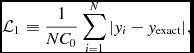 $$\begin{eqnarray}
{\cal L}_{1} \equiv \frac{1}{N C_0}\sum _{i=1}^{N} \vert y_{i} - y_{\rm exact} \vert ,
\end{eqnarray}$$
$$\begin{eqnarray}
{\cal L}_{1} \equiv \frac{1}{N C_0}\sum _{i=1}^{N} \vert y_{i} - y_{\rm exact} \vert ,
\end{eqnarray}$$
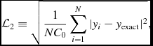 $$\begin{eqnarray}
{\cal L}_{2} \equiv \sqrt{\frac{1}{N C_0}\sum _{i=1}^{N} \vert y_{i} - y_{\rm exact} \vert ^{2}},
\end{eqnarray}$$
$$\begin{eqnarray}
{\cal L}_{2} \equiv \sqrt{\frac{1}{N C_0}\sum _{i=1}^{N} \vert y_{i} - y_{\rm exact} \vert ^{2}},
\end{eqnarray}$$
where y exact is the exact or comparison solution interpolated or computed at the location of each particle i and N is the number of points. The norms are the standard error norms divided by a constant, which we set to the maximum value of the exact solution within the domain, C 0 = max(y exact), in order to give a dimensionless quantity. Otherwise quoting the absolute value of  ${\cal L}_{1}$ or ${\cal L}_{2}$ is meaningless. Dividing by a constant has no effect when considering convergence properties. These are the default error norms computed by splash (Price Reference Price2007).
Achieving formal convergence in SPH is more complicated than in mesh-based codes where linear consistency is guaranteed (see Price Reference Price2012a). The best that can be achieved with regular (positive, symmetric) kernels is second-order accuracy away from shocks provided the particles remain well ordered (Monaghan Reference Monaghan1992). The degree to which this remains true depends on the smoothing kernel and the number of neighbours. Our tests demonstrate that formal second-order convergence can be achieved with Phantom on certain problems (e.g. Section 5.6.1). More typically, one obtains something between first- and second-order convergence in smooth flow depending on the degree of spatial disordering of the particles. The other important difference compared to mesh-based codes is that there is no intrinsic numerical dissipation in SPH due to its Hamiltonian nature—numerical dissipation terms must be explicitly added. We perform all tests with these terms included.
We use timestep factors of C Cour = 0.3 and C force = 0.25 by default for all tests (Section 2.3.2).
5.1. Hydrodynamics
5.1.1. Sod shock tube
Figure 8 shows the results of the standard Sod (Reference Sod1978) shock tube test, performed in 3D using [ρ, P] = [1, 1] in the ‘left state’ (x ⩽ 0) and [ρ, P] = [0.125, 0.1] for the ‘right state’ (x > 0) with a discontinuity initially at x = 0 and zero initial velocity and magnetic field. We perform the test using an adiabatic EOS with γ = 5/3 and periodic boundaries in y and z. While many 1D solutions appear in the literature, only a handful of results on this test have been published for SPH in 3D (e.g. Dolag et al. Reference Dolag, Vazza, Brunetti and Tormen2005; Hubber et al. Reference Hubber, Batty, McLeod and Whitworth2011; Beck et al. Reference Beck2016; a 2D version is shown in Price Reference Price2012a). The tricky part in a 3D SPH code is how to set up the density contrast. Setting particles on a cubic lattice is a poor choice of initial condition since this is not a stable arrangement for the particles (Morris Reference Morris1996b, Reference Morris1996a; Lombardi et al. Reference Lombardi, Sills, Rasio and Shapiro1999; Børve et al. Reference Børve, Omang and Trulsen2004). The approach taken in Springel (Reference Springel2005) (where only the density was shown, being the easiest to get right) was to relax the two halves of the box into a stable arrangement using the gravitational force run with a minus sign, but this is time consuming.
Results of the Sod shock tube test in 3D, showing projection of all particles (black dots) compared to the analytic solution (red line). The problem is set up with [ρ, P] = [1, 1] for x ⩽ 0 and [ρ, P] = [0.125, 0.1] for x > 0 with γ = 5/3, with zero velocities and no magnetic field. The density contrast is initialised using equal mass particles placed on a close packed lattice with 256 × 24 × 24 particles initially in x ∈ [− 0.5, 0] and 128 × 12 × 12 particles initially in x ∈ [0, 0.5]. The results are shown with constant αAV = 1.
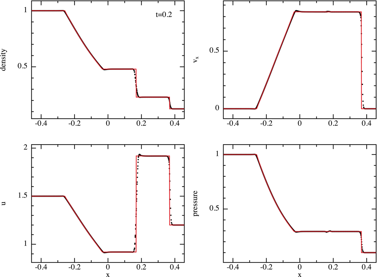
Here we take a simpler approach which is to set the particles initially on a close-packed lattice (Section 3.1), since this is close to the relaxed arrangement (e.g. Lombardi et al. Reference Lombardi, Sills, Rasio and Shapiro1999). To ensure continuity of the lattice across periodic boundaries, we fix the number of particles in the y (z) direction to the nearest multiple of 2 (3) and adjust the spacing in the x-direction accordingly to give the correct density in each subdomain. We implement the boundary condition in the x-direction by tagging the first and last few rows of particles in the x direction as boundary particles, meaning that their particle properties are held constant. The results shown in Figure 8 use 256 × 24 × 24 particles initially in x ∈ [− 0.5, 0] and 128 × 12 × 12 particles in x ∈ [0, 0.5] with code defaults for the artificial conductivity [αu = 1 with vu sig given by equation (43)] and artificial viscosity (αAV = 1, βAV = 2). The results are identical whether global or individual particle timesteps (Section 2.3.4) are used. Figure 9 shows the results when code defaults for viscosity are also employed, resulting in a time-dependent αAV (see lower right panel). There is more noise in the velocity field around the contact discontinuity in this case, but the results are otherwise identical.
As in Figure 8, but with code defaults for all dissipation terms (αAV ∈ [0, 1]; αu = 1). These leave more noise in the velocity field behind the shock but provide second-order convergence in smooth flow. The lower right panel in this case shows the resultant values for the viscosity parameter αAV.
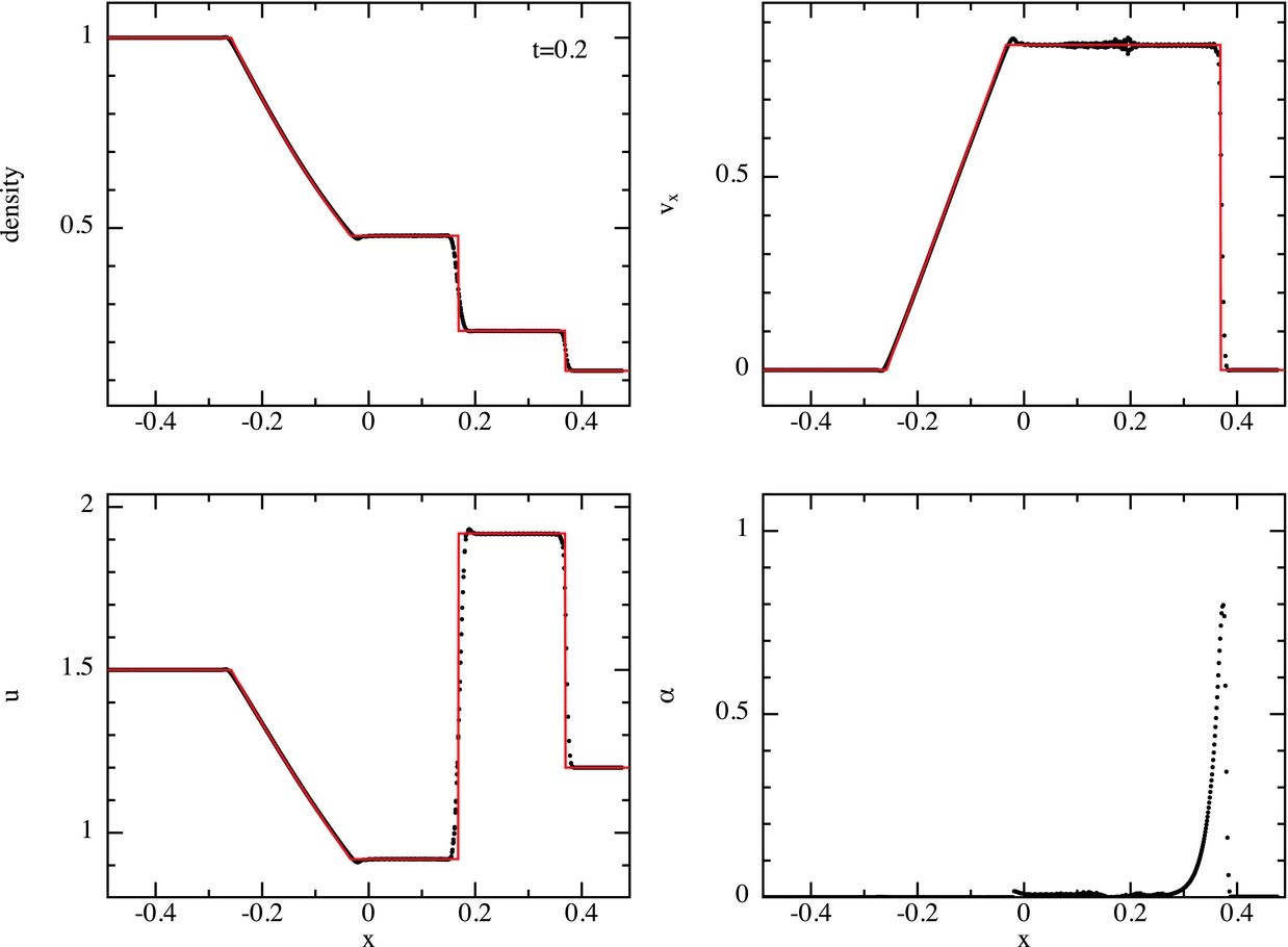
The  ${\cal L}_2$ errors for the solutions shown in Figure 8 are 0.0090, 0.0022, 0.0018, and 0.0045 for the density, velocity, thermal energy, and pressure, respectively. With dissipation switches turned on (Figure 9), the corresponding errors are 0.009, 0.0021, 0.0019, and 0.0044, respectively. That is, our solutions are within 1% of the analytic solution for all four quantities in both cases, with the density profile showing the strongest difference (mainly due to smoothing of the contact discontinuity).
Puri & Ramachandran (Reference Puri and Ramachandran2014) compared our shock capturing algorithm with other SPH variants, including Godunov SPH. Our scheme was found to be the most robust of those tested.
5.1.2. Blast wave
As a more extreme version of the shock test, Figures 10 and 11 show the results of the blast wave problem from Monaghan (Reference Monaghan1997), set up initially with [ρ, P] = [1, 1000] for x ⩽ 0 and [ρ, P] = [1.0, 0.1] for x > 0 and with γ = 1.4 (appropriate to air). As previously, we set the particles on a close-packed lattice with a discontinuous initial pressure profile. We employ 800 × 12 × 12 particles in the domain x ∈ [− 0.5, 0.5]. Results are shown at t = 0.01. This is a more challenging problem than the Sod test due to the higher Mach number. As previously, we show results with both αAV = 1 (Figure 10) and with the viscosity switch α ∈ [0, 1]. Both calculations use αu = 1 with (43) for the signal speed in the artificial conductivity. For the solution shown in Figure 10, we find normalised  ${\cal L}_2$ errors of 0.057, 0.063, 0.051, and 0.018 in the density, velocity, thermal energy, and pressure, respectively, compared to the analytic solution. Employing switches (Figure 11), we find corresponding ${\cal L}_2$ errors of 0.056, 0.059, 0.052, and 0.017. That is, our solutions are within 6% of the analytic solution at this resolution.
Results of the 3D blast wave test, showing projection of all particles (black dots) compared to the analytic solution (red line). The problem is set up with [ρ, P] = [1, 1000] for x ⩽ 0 and [ρ, P] = [1, 0.1] for x > 0 with γ = 7/5, with zero velocities and no magnetic field. We use equal mass particles placed on a close packed lattice with 800 × 12 × 12 particles initially in x ∈ [− 0.5, 0.5]. Results are shown with constant αAV = 1.
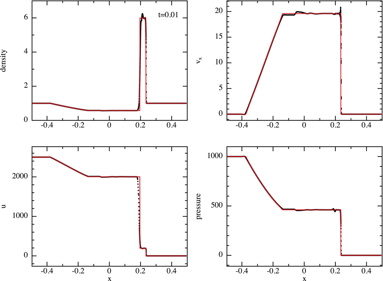
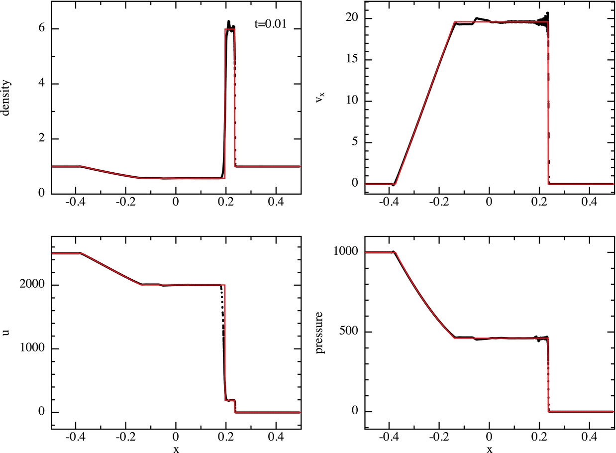
The main source of error is that the contact discontinuity is over-smoothed due to the artificial conductivity, while the velocity profile shows a spurious jump at the location of the contact discontinuity. This glitch is a startup error caused by our use of purely discontinuous initial conditions—it could be removed by adopting smoothed initial conditions but we prefer to perform the more difficult version of this test. There is also noise in the post-shock velocity profile because the viscosity switch does not apply enough dissipation here. As in the previous test, this noise can be reduced by increasing the numerical viscosity, e.g. by adopting a constant αAV (compare Figures 10 and 11).
Figure 12 quantifies the error in energy conservation, showing the error in the total energy as a function of time, i.e. |E − E 0|/|E 0|. Energy is conserved to a relative accuracy of better than 2 × 10⁻⁶.
Relative error in energy conservation for the 3D blast wave test. Energy is conserved to an error of 10−6 in this test.
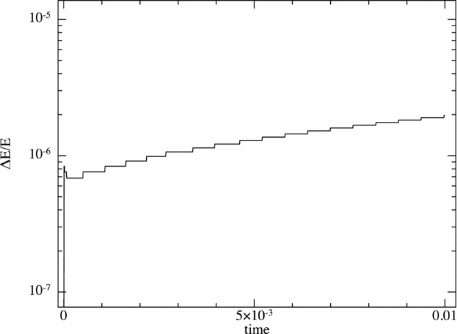
5.1.3. Sedov blast wave
The Sedov–Taylor blast wave (Taylor Reference Taylor1950a, Reference Taylor1950b; Sedov Reference Sedov1959) is a similar test to the previous but with a spherical geometry. This test is an excellent test for the individual timestepping algorithm, since it involves propagating a blast wave into an ambient medium of ‘inactive’ or ‘asleep’ particles, which can cause severe loss of energy conservation if they are not carefully awoken (Saitoh & Makino Reference Saitoh and Makino2009). For previous uses of this test with SPH, see e.g. Springel & Hernquist (Reference Springel and Hernquist2002) and Rosswog & Price (Reference Rosswog and Price2007), and for a comparison between SPH and mesh codes on this test, see Tasker et al. (Reference Tasker, Brunino, Mitchell, Michielsen, Hopton, Pearce, Bryan and Theuns2008).
We set up the problem in a uniform periodic box x, y, z ∈ [− 0.5, 0.5], setting the thermal energy on the particles to be non-zero in a barely resolved sphere around the origin. We assume an adiabatic EOS with γ = 5/3. The total energy is normalised such that the total thermal energy in the blast is E 0 = ∑am au a = 1, distributed on the particles within r < R kernh 0 using the smoothing kernel, i.e.
 $$\begin{equation}
u_{a} = \left\lbrace \arraycolsep5pt\begin{array}{@{}ll@{}}E_{0}W(r, h_{0}), & r/h_{0} \le R_{\rm kern}\\
0 & r/h_{0} > R_{\rm kern}, \end{array}\right.
\end{equation}$$
$$\begin{equation}
u_{a} = \left\lbrace \arraycolsep5pt\begin{array}{@{}ll@{}}E_{0}W(r, h_{0}), & r/h_{0} \le R_{\rm kern}\\
0 & r/h_{0} > R_{\rm kern}, \end{array}\right.
\end{equation}$$
where  $r = \sqrt{x^{2} + y^{2} + z^{2}}$ is the radius of the particle and we set h 0 to be twice the particle smoothing length.
We simulate the Sedov blast wave using both global and individual timesteps at several different resolutions. Figure 13 shows the evolution of the relative error in total energy for our suite, while Figure 14 shows the density at t = 0.1 compared to the analytical solution given by the solid line. Energy is conserved to better than 1% in all cases. Using higher spatial resolution results in a better match of the post-shock density with the analytic solution. The scatter at the leading edge of the shock is a result of the default artificial conductivity algorithm. Given the initial strong gradient in thermal energy, using more artificial conductivity than our switch permits would reduce the noise on this problem (Rosswog & Price Reference Rosswog and Price2007).
Evolution of the relative error in total energy for the Sedov blast wave problem. Resolutions are given in the legend; solid lines use individual timestepping while dotted lines show global timestepping.
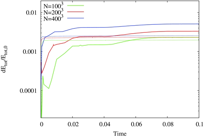
Density as a function of radius in the Sedov blast wave problem at three resolutions. All particles are placed initially on a closepacked lattice, are evolved using individual timesteps and we use the quintic kernel. The analytic solution is given by the solid line, and the bottom panels show the residuals compared to the analytical solution.
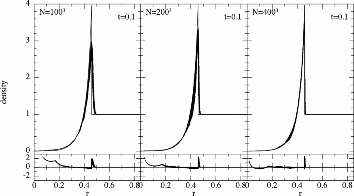
5.1.4. Kelvin–Helmholtz instability
Much has been written about Kelvin–Helmholtz instabilities with SPH (e.g. Agertz et al. Reference Agertz2007; Price Reference Price2008; Abel Reference Abel2011; Valdarnini Reference Valdarnini2012; Read & Hayfield Reference Read and Hayfield2012; Hubber, Falle, & Goodwin Reference Hubber, Falle and Goodwin2013c). For the present purpose, it suffices to say that the test problems considered by Agertz et al. (Reference Agertz2007) and Price (Reference Price2008) are not well posed. That is, the number of small-scale secondary instabilities will always increase with numerical resolution because high wavenumber modes grow fastest in the absence of physical dissipation or other regularising forces such as magnetic fields or surface tension. The ill-posed nature of the test problem has been pointed out by several authors (Robertson et al. Reference Robertson, Kravtsov, Gnedin, Abel and Rudd2010; McNally, Lyra, & Passy Reference McNally, Lyra and Passy2012; Lecoanet et al. Reference Lecoanet2016), who have each proposed well-posed alternatives.
We adopt the setup from Robertson et al. (Reference Robertson, Kravtsov, Gnedin, Abel and Rudd2010), similar to the approach by McNally et al. (Reference McNally, Lyra and Passy2012), where the initial density contrast is smoothed using a ramp function. This should suppress the formation of secondary instabilities long enough to allow a single large-scale mode to grow. The density and shear velocity in the y direction are given by
 $$\begin{equation}
\rho (y) = \rho _{1} + R(y)[\rho _{2} - \rho _{1}],
\end{equation}$$
$$\begin{equation}
\rho (y) = \rho _{1} + R(y)[\rho _{2} - \rho _{1}],
\end{equation}$$
and
 $$\begin{equation}
v_{x}(y) = v_{1} + R(y)[v_{2} - v_{1}],
\end{equation}$$
$$\begin{equation}
v_{x}(y) = v_{1} + R(y)[v_{2} - v_{1}],
\end{equation}$$
where ρ1 = 1, ρ2 = 2, v 1 = −0.5, and v 2 = 0.5 with constant pressure P = 2.5, γ = 5/3. The ramp function is given by
 $$\begin{equation}
R(y) \equiv \left[1 - f(y)\right]\left[1 -g(y)\right],
\end{equation}$$
$$\begin{equation}
R(y) \equiv \left[1 - f(y)\right]\left[1 -g(y)\right],
\end{equation}$$
where
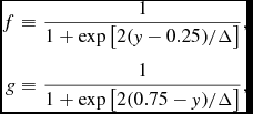 $$\begin{eqnarray}
f & \equiv& \frac{1}{1 + \exp \left[2(y-0.25)/\Delta \right]}, \nonumber \\
g & \equiv& \frac{1}{1 + \exp \left[2(0.75-y)/\Delta \right]},
\end{eqnarray}$$
$$\begin{eqnarray}
f & \equiv& \frac{1}{1 + \exp \left[2(y-0.25)/\Delta \right]}, \nonumber \\
g & \equiv& \frac{1}{1 + \exp \left[2(0.75-y)/\Delta \right]},
\end{eqnarray}$$
and we set Δ = 0.25. Finally, a perturbation is added in the velocity in the y direction, given by
 $$\begin{equation}
v_{y} = 0.1 \sin (2\pi x).
\end{equation}$$
$$\begin{equation}
v_{y} = 0.1 \sin (2\pi x).
\end{equation}$$
The setup in Robertson et al. (Reference Robertson, Kravtsov, Gnedin, Abel and Rudd2010) is 2D, but since Phantom is a 3D code, we instead set up the problem using a thin 3D box. We first set up a uniform close packed lattice in a periodic box with dimensions  $1 \times 1 \times \sqrt{24}/n_{x}$, where n x is the initial resolution in the x direction such that the box thickness is set to be exactly 12 particle spacings in the z direction independent of the resolution used in the x and y direction. The box is set between [0,1] in x and y, consistent with the ramp function. We then set up the density profile by stretch mapping in the y direction using (312) as the input function (c.f. Section 3.2).
Figure 15 shows the results of this test, showing a cross section of density at z = 0 for three different resolutions (top to bottom) and at the times corresponding to those shown in Robertson et al. (Reference Robertson, Kravtsov, Gnedin, Abel and Rudd2010). We compute the quantitative difference between the calculations by taking the root mean square difference of the cross section slices shown above interpolated to a 1,024 × 1,024 pixel map. The error between the n x = 64 calculation and the n x = 256 calculation is 1.3 × 10⁻³, while this reduces to 4.9 × 10⁻⁴ for the n x = 128 calculation. Figure 16 shows the growth of the amplitude of the mode seeded in (316). We follow the procedure described in McNally et al. (Reference McNally, Lyra and Passy2012) to calculate the mode amplitude. At t = 2, the amplitude between the n x = 128 and n x = 256 calculations is within 4%. The artificial viscosity and conductivity tend to slow convergence on this problem, so it is a good test of the dissipation switches (we use the default code viscosity switch as discussed in Section 2.2.9).
Results of the well-posed Kelvin–Helmholtz instability test from Robertson et al. (Reference Robertson, Kravtsov, Gnedin, Abel and Rudd2010), shown at a resolution of (from top to bottom) 64 × 74 × 12, 128 × 148 × 12 and 256 × 296 × 12 equal mass SPH particles. We use stretch mapping (Section 3.2) to achieve the initial density profile, consisting of a 2:1 density jump with a smoothed transition.
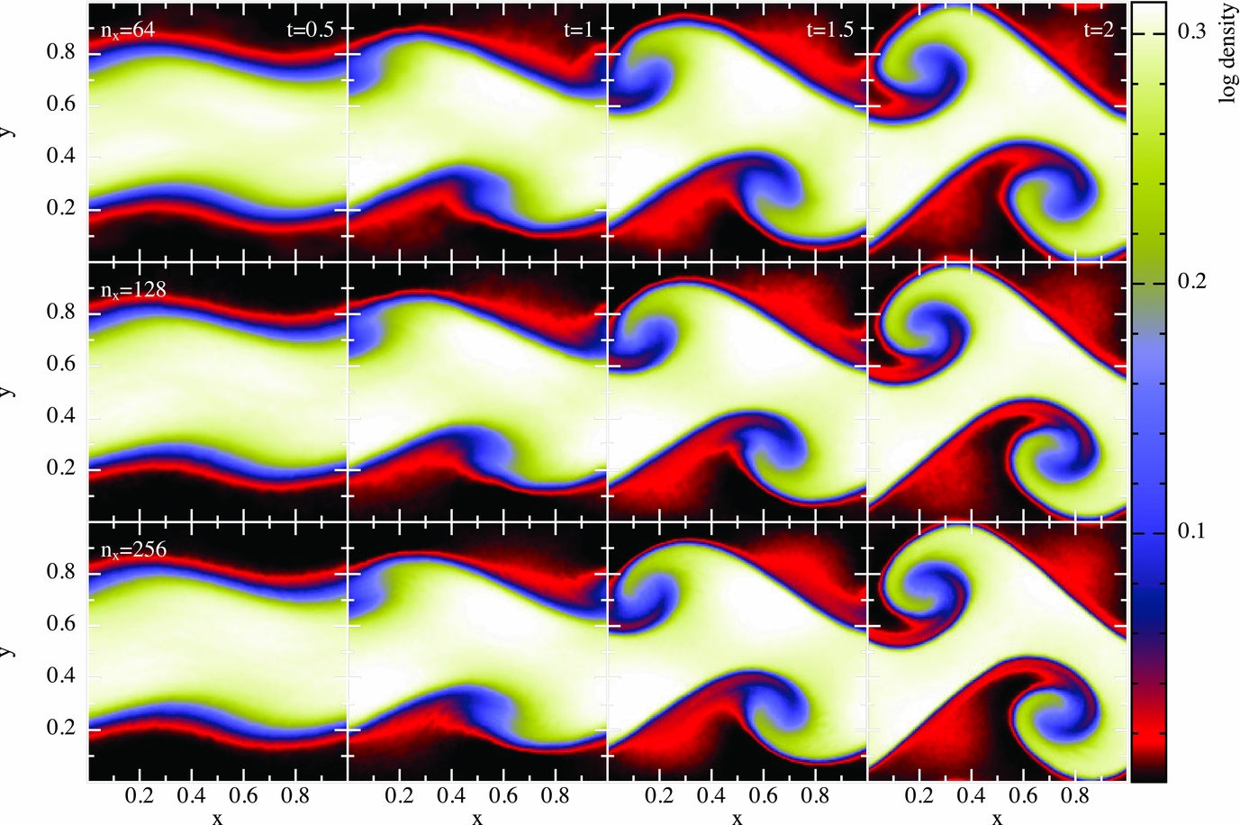
Growth of the amplitude of the seeded mode for the Kevin–Helmholtz instability test. The amplitude at t = 2 between the n x = 128 and n x = 256 calculations is within 4%.
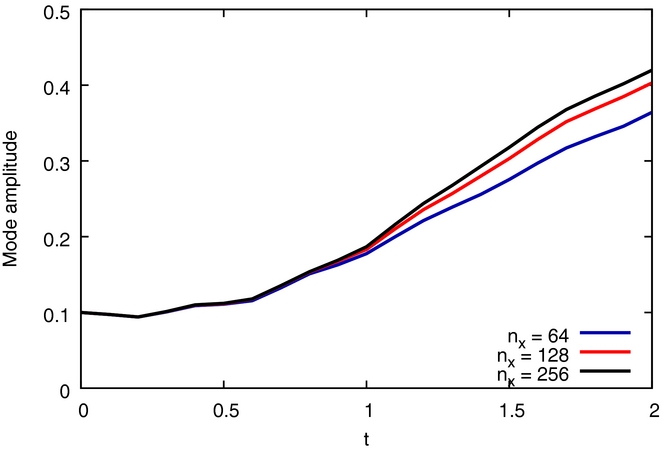
5.2. External forces
5.2.1. Lense–Thirring precession
We test the implementation of the Lense–Thirring precession by computing the precession induced on a pressure-less disc of particles, as outlined in Nealon et al. (Reference Nealon, Price and Nixon2015). This disc is simulated for one orbit at the outer edge such that the inner part of the disc has precessed multiple times but the outer region has not yet completed a full precession. The precession timescale is estimated by measuring the twist as a function of time for each radial bin; in the inner region, this is the time taken for the twist to go from a minimum (zero twist) to a maximum (fully twisted) and in the outer region the gradient of the twist against time is used to calculate the equivalent time. Figure 17 shows the precession timescale measured from the simulation as a function of the radius compared to the analytically derived precession timescale, with uncertainties derived from the calculation of the gradient.
Lense–Thirring precession test from a disc inclined by 30°. Here, the precession timescale is measured from the cumulative twist in the disc and the exact solution, t p = R 3/2a is represented by the red line.
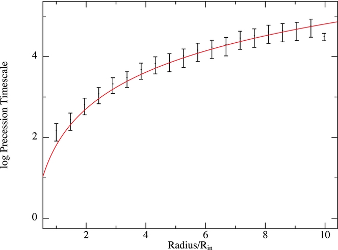
5.2.2. Poynting–Robertson drag
Figure 18 shows the trajectory of a spherical assembly of 89 pressureless SPH particles subject to Poynting–Robertson drag with a fixed value of βPR = 0.1, assuming a central neutron star of mass 1.4 M⊙ and 10 km radius and a particle initially orbiting at R = 200 km with initial v ϕ of 0.9 times the Keplerian orbital speed. We compare this to the trajectory of a test particle produced by direct numerical integration of the equations of motion, (106), with a fourth-order Runge Kutta scheme. As shown in Figure 18, there is no significant difference between the codes. We therefore expect that the behaviour of SPH gas or dust particles under the influence of any given β will be correct.
Inspiral of a test particle subjected to Poynting–Robertson drag using Phantom (blue curve) compared to the expected solution (red curve). For clarity, only some of the points are plotted. The results are indistinguishable on this scale. Bottom panel shows the distance (Δr) between the PHANTOM particle and the test code particle. This demonstrates that the implementation of Poynting–Robertson drag in Phantom is consistent with a fourth-order numerical solution to (106).

5.2.3. Galactic potentials
Figure 19 shows six calculations with gas embedded within different galactic potentials (Section 2.4.4). We set up an isothermal gas disc with T = 10 000 K, with a total gas mass of 1 × 10⁹ M⊙ set up in a uniform surface density disc from 0–10 kpc in radius. A three-part potential model for the Milky Way provides the disc with an axisymmetric rotation curve [bulge plus disc plus halo, the same as Pettitt et al. (Reference Pettitt, Dobbs, Acreman and Price2014)]. The top row shows gas exposed to spiral potentials of Cox & Gómez (Reference Cox and Gómez2002) with three different arm numbers (2, 3, and 4), while the bottom row shows simulations within the bar potential of Wada & Koda (Reference Wada and Koda2001) at three different pattern speeds (40, 60, and 80 km s−1 kpc−1). All models are shown after approximately one full disc rotation (240 Myr). Gas can be seen to trace the different spiral arm features, with the two armed model in particular showing branches characteristic of such density wave potentials (e.g. Martos et al. Reference Martos, Hernandez, Yáñez, Moreno and Pichardo2004). The bars drive arm features in the gas, the radial extent of which is a function of the pattern speed. Also, note the inner elliptical orbits of the bar at the location of the Lindblad resonance which is an effect of the peaked inner rotation curve resulting from the central bulge.
Gas in a galactic disc under the effect of different galactic potentials. Top row shows models with a 2, 3, and 4 armed spiral (left to right) with a pitch angle of 15° and pattern speed of 20 km s−1 kpc−1. Bottom row shows a bar potential with pattern speeds of 40, 60, and 80 km s−1 kpc−1 (left to right).
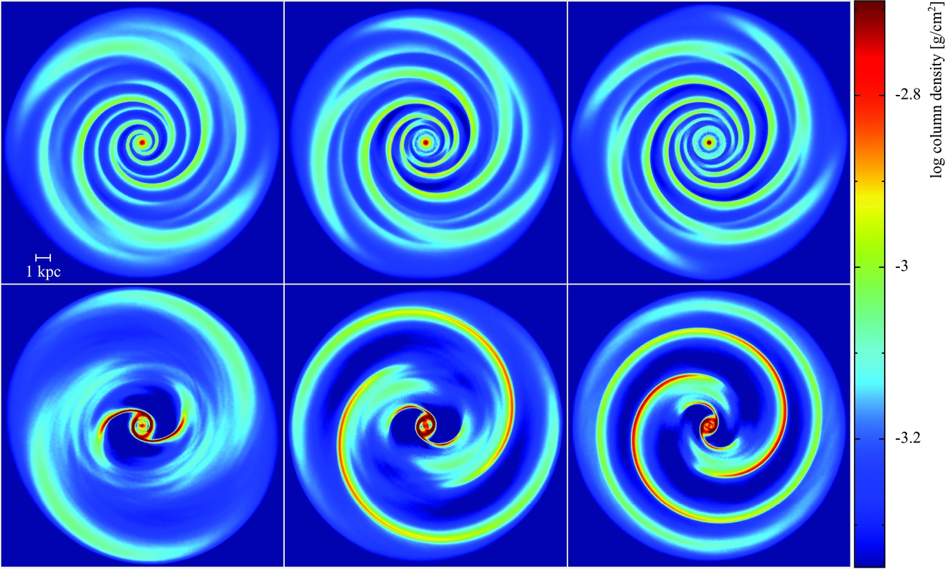
5.3. Accretion discs
SPH has been widely used for studies of accretion discs, ever since the first studies by Artymowicz & Lubow (Reference Artymowicz and Lubow1994, Reference Artymowicz and Lubow1996), Murray (Reference Murray1996), and Maddison, Murray, & Monaghan (Reference Maddison, Murray and Monaghan1996) showed how to use the SPH artificial viscosity term to mimic a Shakura & Sunyaev (Reference Shakura and Sunyaev1973) disc viscosity.
5.3.1. Measuring the disc viscosity
The simplest test is to measure the disc viscosity from the diffusion rate of the disc surface density. Figure 20 shows the results of an extensive study of this with Phantom perfomed by Lodato & Price (Reference Lodato and Price2010). For this study, we set up a disc from R in = 0.5 to R out = 10 with surface density profile
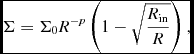 $$\begin{equation}
\Sigma = \Sigma _0 R^{-p} \left( 1 - \sqrt{\frac{R_{\rm in}}{R}} \right),
\end{equation}$$
$$\begin{equation}
\Sigma = \Sigma _0 R^{-p} \left( 1 - \sqrt{\frac{R_{\rm in}}{R}} \right),
\end{equation}$$
and a locally isothermal EOS c s = c s, 0R −q. We set p = 3/2 and q = 3/4 such that the disc is uniformly resolved, i.e. h/H ~ constant (Lodato & Pringle Reference Lodato and Pringle2007), giving a constant value of the Shakura & Sunyaev (Reference Shakura and Sunyaev1973) α parameter according to (124). We set c s, 0 such that the aspect ratio is H/R = 0.02 at R = 1. We used 2 million particles by default, with several additional calculations performed using 20 million particles. The simulation is performed to t = 1,000 in code units.
Calibration of the disc viscosity in Phantom, comparing the input value of the Shakura–Sunyaev α from (124) (x-axis) with the measured diffusion rate of the surface density by fitting to a 1D code (y-axis). Triangles indicate simulations with the disc viscosity computed using the artificial viscosity (Section 2.6.1), while squares represent simulations using physical viscosity (Section 2.7.1). All simulations use 2 million particles except for the green, cyan, and red triangles which use 20 million particles. Figure taken from Lodato & Price (Reference Lodato and Price2010).
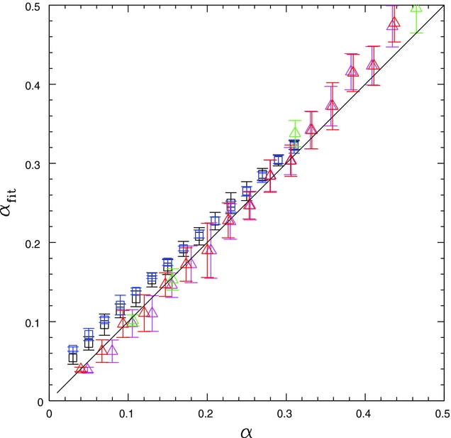
The diffusion rate is measured by fitting the surface density evolution obtained from Phantom with the results of a ‘ring code’ solving the standard 1D diffusion equation for accretion discs (Lynden-Bell & Pringle Reference Lynden-Bell and Pringle1974; Pringle Reference Pringle1981, Reference Pringle1992). Details of the fitting procedure are given in Lodato & Price (Reference Lodato and Price2010). In short, we use Newton–Raphson iterations to find the minimum error between the 1D code and the surface density profile from Phantom at the end of the simulation, which provides the best fit (αfit) and error bars. Figure 20 shows that the measured diffusion rates agree with the expected values to within the error bars. The exception is for low viscosity discs with physical viscosity, where contribution from artificial viscosity becomes significant. Triangles in the figure show the results with disc viscosity computed from the artificial viscosity (Section 2.6.1), while squares represent simulations with physical viscosity set according to (126).
This test demonstrates that the implementation of disc viscosity matches the analytic theory to within measurement errors. This also demonstrates that the translation of the artificial viscosity term according to (124) is correct.
5.3.2. Warp diffusion
A more demanding test of disc physics involves the dynamics of warped discs. Extensive analytic theory exists, starting with the linear theory of Papaloizou & Pringle (Reference Papaloizou and Pringle1983), subsequent work by Pringle (Reference Pringle1992), and culminating in the work by Ogilvie (Reference Ogilvie1999) which provides the analytic expressions for the diffusion rate of warps in discs for non-linear values of both disc viscosity and warp amplitude. Importantly, this theory applies in the ‘diffusive’ regime where the disc viscosity exceeds the aspect ratio, α > H/R. For α ≲ H/R, the warp propagation is wave-like and no equivalent non-linear theory exists (see Lubow & Ogilvie Reference Lubow and Ogilvie2000; Lubow, Ogilvie, & Pringle Reference Lubow, Ogilvie and Pringle2002).
Phantom was originally written to simulate warped discs—with our first study in Lodato & Price (Reference Lodato and Price2010) designed to test the Ogilvie (Reference Ogilvie1999) theory in 3D simulations. Figure 21 shows the results of this study, showing the measured warp diffusion rate as a function of disc viscosity. The setup of the simulations is as in the previous test but with a small warp added to the disc, as outlined in Section 3.3 of Lodato & Price (Reference Lodato and Price2010). Details of the fitting procedure used to measure the warp diffusion rate are also given in Section 4.2 of that paper. The dashed line shows the non-linear prediction of Ogilvie (Reference Ogilvie1999), namely
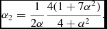 $$\begin{equation}
\alpha _2 = \frac{1}{2\alpha } \frac{4(1 + 7\alpha ^2)}{4 + \alpha ^2}.
\end{equation}$$
$$\begin{equation}
\alpha _2 = \frac{1}{2\alpha } \frac{4(1 + 7\alpha ^2)}{4 + \alpha ^2}.
\end{equation}$$
Significantly, the Phantom results show a measurable difference between the predictions of the non-linear theory and the prediction from linear theory (Papaloizou & Pringle Reference Papaloizou and Pringle1983) of α2 = 1/(2α), shown by the solid black line.
Warp diffusion rate as a function of disc viscosity, showing the Phantom results compared to the non-linear theory of Ogilvie (Reference Ogilvie1999) (dashed line). The linear prediction, α2 = 1/(2α), is shown by the solid line, highlighting the agreement of Phantom with the non-linear theory. Colouring of points is as in Figure 20. Figure taken from Lodato & Price (Reference Lodato and Price2010).
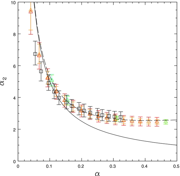
In addition to the results shown in Figure 21, Phantom also showed a close match to both the predicted self-induced precession of the warp and to the evolution of non-linear warps (see Figures 13 and 14 in Lodato & Price Reference Lodato and Price2010, respectively). From the success of this initial study, we have used Phantom to study many aspects of disc warping, either with isolated warps or breaks (Lodato & Price Reference Lodato and Price2010; Nixon et al. Reference Nixon, King and Price2012a), warps induced by spinning black holes (Nixon et al. Reference Nixon, King, Price and Frank2012b; Nealon et al. Reference Nealon, Price and Nixon2015, Reference Nealon, Nixon, Price and King2016), and warps in circumbinary (Nixon et al. Reference Nixon, King and Price2013; Facchini et al. Reference Facchini, Lodato and Price2013) or circumprimary (Doğan et al. Reference Doğan, Nixon, King and Price2015; Martin et al. Reference Martin, Nixon, Armitage, Lubow and Price2014a, Reference Martin, Nixon, Lubow, Armitage, Price, Doğan and King2014b) discs. In particular, Phantom was used to discover the phenomenon of ‘disc tearing’ where sections of the disc are ‘torn’ from the disc plane and precess effectively independently (Nixon et al. Reference Nixon, King, Price and Frank2012b, Reference Nixon, King and Price2013; Nealon et al. Reference Nealon, Price and Nixon2015).
5.3.3. Disc–planet interaction
Although there is no ‘exact’ solution for planet–disc interaction, an extensive code comparison was performed by de Val-Borro et al. (Reference de Val-Borro2006). Figure 22 shows the column density of a 3D Phantom calculation, plotted in r–ϕ with the density integrated through the z direction, comparable to the ‘viscous Jupiter’ setup in de Val-Borro et al. (Reference de Val-Borro2006).
Planet–disc interaction in 3D, showing the ‘viscous Jupiter’ calculation comparable to the 2D results shown with various grid and SPH codes in Figure 10 of de Val-Borro et al. (Reference de Val-Borro2006). The dotted lines shows the estimated position of the planetary shocks from Ogilvie & Lubow (Reference Ogilvie and Lubow2002). The offset between this solution and the numerical shock position is due to the approximate nature of the analytic solution (see de Val-Borro et al. Reference de Val-Borro2006).
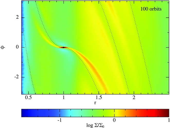
Two caveats apply when comparing our results with those in Figure 10 of de Val-Borro et al. (Reference de Val-Borro2006). The first is that the original comparison project was performed in 2D and mainly with grid-based codes with specific ‘wave damping’ boundary conditions prescribed. We chose simply to ignore the prescribed boundary conditions and two dimensionality and instead modelled the disc in 3D with a central accretion boundary at r = 0.25 with a free outer boundary, with the initial disc set up from r = 0.4 to r = 2.5. We used 106 SPH particles. Second, the planetary orbit was prescribed on a fixed circular orbit with no accretion onto either the planet or the star. Although we usually use sink particles in Phantom to model planet–disc interaction (e.g. Dipierro et al. Reference Dipierro, Price, Laibe, Hirsh and Cerioli2015), for this test we thus employed the fixed binary potential (Section 2.4.2) to enable a direct comparison. We thus used M = 10−3 in the binary potential, corresponding to the ‘Jupiter’ simulation in de Val-Borro et al. (Reference de Val-Borro2006) with the planet on a fixed circular orbit at r = 1.
As per the original comparison project, we implemented Plummer softening of the gravitational force from the planet
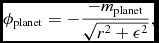 $$\begin{equation}
\phi _{\rm planet} = - \frac{-m_{\rm planet}}{\sqrt{r^{2} + \epsilon ^{2}}},
\end{equation}$$
$$\begin{equation}
\phi _{\rm planet} = - \frac{-m_{\rm planet}}{\sqrt{r^{2} + \epsilon ^{2}}},
\end{equation}$$
where ε = 0.6H. We also implemented the prescribed increase of planet mass with time for the first five orbits according to
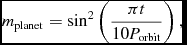 $$\begin{equation}
m_{\rm planet} = \sin ^{2} \left( \frac{\pi t}{10 P_{\rm orbit}} \right),
\end{equation}$$
$$\begin{equation}
m_{\rm planet} = \sin ^{2} \left( \frac{\pi t}{10 P_{\rm orbit}} \right),
\end{equation}$$
where P orbit is the orbital period (2π in code units), though we found this made little or no difference to the results in practice. We assumed a locally isothermal EOS, c s∝R −0.5, such that H/R ≈ 0.05 ≈ constant. We assumed an initially constant surface density, Σ0 = 0.002 M */(πa 2). We also employed a Navier–Stokes viscosity with ν = 10−5 on top of the usual settings for shock dissipation with the viscosity switch, namely αAV ∈ [0, 1] and βAV = 2. We use the Navier–Stokes viscosity implementation described in Section 2.7.2, which is the code default. We also employed the cubic spline kernel (with h fac = 1.2) rather than the quintic to reduce the computational expense (using the quintic made no difference to the results).
Despite the different assumptions, the results in Figure 22 are strikingly similar to those obtained with most of the grid-based codes in de Val-Borro et al. (Reference de Val-Borro2006). The main difference is that our gap is shallower, which is not surprising since this is where resolution is lowest in SPH. There is also some difference in the evolution of the surface density, particularly at the inner boundary, due to the difference in assumed boundary conditions. However, the dense flow around the planet and in the shocks appear well resolved compared to the other codes. What is interesting is that the SPH codes used in the original comparison performed poorly on this test. This may be simply due to the low resolution employed, as the two SPH calculations used 250 000 and 300 000 particles, respectively, (though performed only in 2D rather than 3D), but given the extent of other differences between adopted setup and SPH algorithms, it is hard to draw firm conclusions.
As per the original comparison, Figure 22 shows the estimated position of the planetary shocks from Ogilvie & Lubow (Reference Ogilvie and Lubow2002) plotted as dotted lines, namely
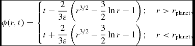 $$\begin{equation}
\phi (r,t) = \left\lbrace \arraycolsep5pt\begin{array}{@{}ll@{}}t - \displaystyle\frac{2}{3 \varepsilon } \left( r^{3/2} - \displaystyle\frac{3}{2} \ln r - 1\right); & r > r_{\rm planet}, \\[8pt]
t + \displaystyle\frac{2}{3 \varepsilon } \left( r^{3/2} - \displaystyle\frac{3}{2} \ln r - 1\right); & r < r_{\rm planet}, \end{array}\right.
\end{equation}$$
$$\begin{equation}
\phi (r,t) = \left\lbrace \arraycolsep5pt\begin{array}{@{}ll@{}}t - \displaystyle\frac{2}{3 \varepsilon } \left( r^{3/2} - \displaystyle\frac{3}{2} \ln r - 1\right); & r > r_{\rm planet}, \\[8pt]
t + \displaystyle\frac{2}{3 \varepsilon } \left( r^{3/2} - \displaystyle\frac{3}{2} \ln r - 1\right); & r < r_{\rm planet}, \end{array}\right.
\end{equation}$$
where ε = 0.05 is the disc aspect ratio. The disagreement between the shock position and the Ogilvie & Lubow (Reference Ogilvie and Lubow2002) solution seen in Figure 22 was also found in every simulation shown in de Val-Borro et al. (Reference de Val-Borro2006), so more likely reflects the approximate nature of the analytic solution rather than numerical error.
We found this to be a particularly good test of the viscosity limiter, since there is both a shock and a shear flow present. Without the limiter in (46), we found the shock viscosity switch would simply trigger to αAV ≈ 1. The original Morris & Monaghan (Reference Morris and Monaghan1997) switch (Section 2.2.9) also performs well on this test, suggesting that the velocity divergence is better able to pick out shocks in differentially rotating discs compared to its time derivative.
5.4. Physical viscosity
5.4.1. Taylor–Green vortex
The Taylor–Green vortex (Taylor & Green Reference Taylor and Green1937) consists of a series of counter-rotating vortices. We perform this test using four vortices set in a thin 3D slab. The initial velocity fields are given by v x = v 0sin(2πx)cos(2πy), v y = −v 0cos(2πx)sin(2πy) with v 0 = 0.1. The initial density is uniform ρ = 1, and an isothermal EOS is used (P = c 2sρ) with speed of sound c s = 1. Viscosity will cause each component of the velocity field to decay at a rate ∝exp(− 16π2νt), where ν is the kinematic shear viscosity.
Figure 23 shows the kinetic energy for a series of calculations using ν = 0.05, 0.1, 0.2. In each case, the kinetic energy exponentially decays by several orders of magnitude. The corresponding analytic solutions are shown by the solid black lines for comparison, demonstrating that the implementation of physical viscosity in Phantom is correct.
Test of physical Navier–Stokes viscosity in the Taylor–Green vortex using kinematic shear viscosity ν = 0.05, 0.1, 0.2. The exponential decay rate of kinetic energy may be compared to the analytic solution in each case (solid black lines), demonstrating that the calibration of physical viscosity in Phantom is correct.
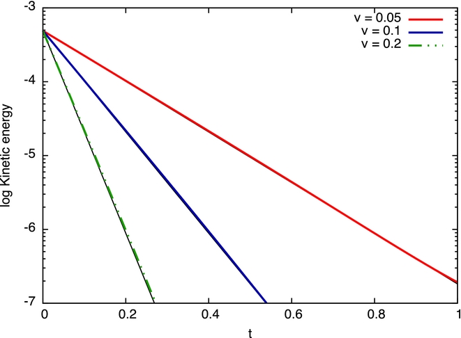
5.5. Sink particles
5.5.1. Binary orbit
Figure 24 shows the error in total energy conservation ΔE/|E 0| for a set of simulations consisting of two sink particles set up in a binary orbit, a common test of N-body integrators (e.g. Hut, Makino, & McMillan Reference Hut, Makino and McMillan1995; Quinn et al. Reference Quinn, Katz, Stadel and Lake1997; Farr & Bertschinger Reference Farr and Bertschinger2007; Dehnen & Read Reference Dehnen and Read2011). We fix the initial semi-major axis a = 1 with masses m 1 = m 2 = 0.5 and with the two sink particles initially at periastron, corresponding to  ${\bm x}_1 = [- m_2/(m_1 + m_2)\Delta ,0,0]$ and ${\bm x}_2 = [m_1/(m_1 + m_2)\Delta ,0,0]$, where Δ = a(1 − e) is the initial separation. The corresponding initial velocities are ${\bm v}_1 = [0,- m_2/(m_1 + m_2)\vert v \vert ,0]$ and ${\bm v}_2 = [0,m_1/(m_1 + m_2)\vert v \vert ,0]$, where $\vert v \vert = \sqrt{a(1-e^2)(m_1 + m_2)}/\Delta$. The orbital period is thus $P = \sqrt{4\pi ^2 a^3 / (G (m_1 + m_2))} = 2\pi$ in code units for our chosen parameters. Importantly, we use an adaptive timestep which is not time symmetric so there remains some drift in the energy error which is absent if the timestep is constant (see e.g. Hut et al. Reference Hut, Makino and McMillan1995; Quinn et al. Reference Quinn, Katz, Stadel and Lake1997 and Dehnen & Read Reference Dehnen and Read2011 for discussion of this issue).
Errors in energy conservation in a sink particle binary integration with code default parameters for the timestep control, showing the energy drift caused by the adaptive timestepping. Angular momentum is conserved to machine precision.

Figure 24 shows the error in total energy as a function of time for the first 1,000 orbits for calculations with initial eccentricities of e = 0.0 (a circular orbit), 0.3, 0.5, 0.7, and 0.9. Energy conservation is worse for more eccentric orbits, as expected, with ΔE/|E 0| ~ 6% after 1,000 orbits for our most extreme case (e = 0.9). The energy error can be reduced arbitrarily by decreasing the timestep, so this is mainly a test of the default settings for the sink particle timestep control. For this problem, the timestep is controlled entirely by (76), where by default we use  $\eta _\Phi = 0.05$, giving 474 steps per orbit for e = 0.9. For simulations with more eccentric orbits, we recommend decreasing C force from the default setting of 0.25 to obtain more accurate orbital dynamics.
In addition to calibrating the timestep constraint, Figure 24 also validates the sink particle substepping via the RESPA algorithm (Section 2.3.3) since for this problem the ‘gas’ timestep is set only by the desired interval between output files (to ensure sufficient output for the figure we choose Δt max = 1, but we also confirmed that this choice is unimportant for the resultant energy conservation). This means that increasing the accuracy of sink particle interactions adds little or no cost to calculations involving gas particles.
The corresponding plot for angular momentum conservation (not shown) merely demonstrates that angular momentum is conserved to machine precision (ΔL/|L| ~ 10−15), as expected. Importantly, angular momentum remains conserved to machine precision even with adaptive timestepping.
5.5.2. Restricted three-body problem
Chin & Chen (Reference Chin and Chen2005) proposed a more demanding test of N-body integrators, consisting of a test particle orbiting in the potential of a binary on a fixed circular orbit. We set up this problem with a single sink particle with  ${\bm x} = [0,0.0580752367,0]$ and ${\bm v} = [0.489765446,0,0]$, using the time-dependent binary potential as described in Section 2.4.2 with M = 0.5. This is therefore a good test of the interaction between a sink particle and external potentials in the code, as well as the sink particle timestepping algorithm. For convenience, we set the sink mass m = 1 and accretion radius r acc = 0.1, although both are irrelevant to the problem.
Figure 25 shows the resulting orbit using the default code parameters, where we plot the trajectory of the sink particle up to t = 27π, as in Figures 1 and 2 of Chin & Chen (Reference Chin and Chen2005). Considering that we use only a second-order integrator, the orbital trajectory is remarkably accurate, showing no chaotic behaviour and only a slight precession consistent or better than the results with some of the fourth-order schemes shown in their paper (albeit computed with a larger timestep). We are thus satisfied that our time integration scheme and the associated timestep settings can capture complex orbital dynamics with sufficient accuracy.
Orbit of a sink particle in the restricted three-body problem from Chin & Chen (Reference Chin and Chen2005) using default code parameters. This tests both the time integrator for sink particles and the interaction with a time-dependent binary potential (Section 2.4.2). The trajectory of the sink is plotted every timestep for three periods (t = 27π).
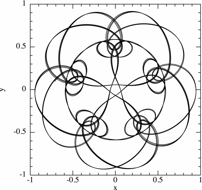
5.6. Magnetohydrodynamics
5.6.1. 3D circularly polarised Alfvén wave
Tóth (Reference Tóth2000) introduced the circularly polarised Alfvén wave test, an exact non-linear solution to the MHD equations which can therefore be performed using a wave of arbitrarily large amplitude. Most results of this test are shown in 2D (e.g. Price & Monaghan Reference Price and Monaghan2005; Rosswog & Price Reference Rosswog and Price2007; Price Reference Price2012a; Tricco & Price Reference Tricco and Price2013). Here we follow the 3D setup outlined by Gardiner & Stone (Reference Gardiner and Stone2008). We use a periodic domain of size L × L/2 × L/2, where L = 3, with the wave propagation direction defined using angles a and b where sina = 2/3 and 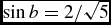 $\sin b = 2/\sqrt{5}$, with the unit vector along the direction of propagation given by ${\bm r} = [\cos a \cos b, \cos a \sin b, \sin a]$. We use an initial density ρ = 1, an adiabatic EOS with γ = 5/3 and P = 0.1. We perform the ‘travelling wave test’ from Gardiner & Stone (Reference Gardiner and Stone2008), where the wavelength λ = 1 and the vectors [v 1, v 2, v 3] = [0, 0.1sin(2πx 1/λ), 0.1cos(2πx 1/λ)] and [B 1, B 2, B 3] = [1, 0.1sin(2πx 1/λ), 0.1cos(2πx 1/λ)] are projected back into the x, y, and z components using the transformations given by (Gardiner & Stone Reference Gardiner and Stone2008)
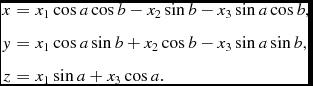 $$\begin{eqnarray}
x & =& x_{1} \cos a \cos b - x_{2} \sin b - x_{3} \sin a \cos b, \nonumber \\
y & =& x_{1} \cos a \sin b + x_{2} \cos b - x_{3} \sin a \sin b, \nonumber \\
z & =& x_{1} \sin a + x_{3} \cos a.
\end{eqnarray}$$
$$\begin{eqnarray}
x & =& x_{1} \cos a \cos b - x_{2} \sin b - x_{3} \sin a \cos b, \nonumber \\
y & =& x_{1} \cos a \sin b + x_{2} \cos b - x_{3} \sin a \sin b, \nonumber \\
z & =& x_{1} \sin a + x_{3} \cos a.
\end{eqnarray}$$
Figure 26 shows the results of this test using 32 × 18 × 18, 64 × 36 × 39 and 128 × 74 × 78 particles initially set on a close packed lattice, compared to the exact solution given by the red line (the same as the initial conditions for the wave). We plot the transverse component of the magnetic field B 2 as a function of x 1, where  $B_{2} \equiv (B_{y}-2B_{x})/\sqrt{5}$ and x 1 ≡ (x + 2y + 2z)/3 for our chosen values of a and b. There is both a dispersive and dissipative error, with the result converging in both phase and amplitude towards the undamped exact solution as the resolution is increased.
Results of the 3D circularly polarised Alfven wave test after five periods, showing perpendicular component of the magnetic field on all particles (black dots) as a function of distance along the axis parallel to the wave vector. Results are shown using 32 × 18 × 18, 64 × 36 × 39, and 128 × 74 × 78 particles (most to least damped, respectively), compared to the exact solution given by the solid red line. Convergence is shown in Figure 27.

Figure 27 shows a convergence study on this problem, showing, as in Gardiner & Stone (Reference Gardiner and Stone2008), the  ${\mathcal{L}}_{1}$ error as a function of the number of particles in the x-direction. The convergence is almost exactly second order. This is significant because we have performed the test with code defaults for all dissipation and divergence cleaning terms. This plot therefore demonstrates the second-order convergence of both the viscous and resistive dissipation in Phantom (see Sections 2.2.9 and 2.10.6). By comparison, the solution shown by Price & Monaghan (Reference Price and Monaghan2005) (Figure 6 in their paper) was severely damped when artificial resistivity was applied.
Convergence in the 3D circularly polarised Alfven wave test, showing the L 1 error as a function of the number of particles along the x-axis, n x alongside the expected slope for second-order convergence (dotted line). Significantly, this demonstrates second-order convergence with all dissipation switched on.
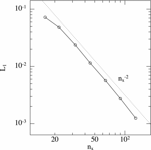
As noted by Price & Monaghan (Reference Price and Monaghan2005) and illustrated in Figure 12 of Price (Reference Price2012a), this problem is unstable to the SPMHD tensile instability (e.g. Phillips & Monaghan Reference Phillips and Monaghan1985) in the absence of force correction terms since the plasma  $\beta \equiv P/ \frac{1}{2} B^{2} \approx 0.2$. Our results demonstrate that the correction term (Section 2.10.2) effectively stabilises the numerical scheme without affecting the convergence properties.
5.6.2. MHD shock tubes
The classic Brio & Wu (Reference Brio and Wu1988) shock tube test generalises the Sod shock tube (Section 5.1.1) to MHD. It has provoked debate over the years (e.g. Wu Reference Wu1988; Dai & Woodward Reference Dai and Woodward1994a; Falle & Komissarov Reference Falle and Komissarov2001; Takahashi, Yamada, & Yamada Reference Takahashi and Yamada2013) because of the presence of a compound slow shock and rarefaction in the solution, which is stable only when the magnetic field is coplanar and there is no perturbation to the tangential (B z) magnetic field (Barmin, Kulikovskiy, & Pogorelov Reference Barmin, Kulikovskiy and Pogorelov1996). Whether or not such solutions can exist in nature remains controversial (e.g. Feng et al. Reference Feng, Lin, Chao, Wu and Lyu2007). Nevertheless, it has become a standard benchmark for numerical MHD (e.g. Stone et al. Reference Stone, Hawley, Evans and Norman1992; Dai & Woodward Reference Dai and Woodward1994a; Balsara Reference Balsara1998; Ryu & Jones Reference Ryu and Jones1995). It was first used to benchmark SPMHD by Price & Monaghan (Reference Price and Monaghan2004a, Reference Price and Monaghan2004b) and 1.5D results on this test with SPMHD, for comparison, can be found in e.g. Price & Monaghan (Reference Price and Monaghan2005), Rosswog & Price (Reference Rosswog and Price2007), Dolag & Stasyszyn (Reference Dolag and Stasyszyn2009), Price (Reference Price2010), and Vanaverbeke, Keppens, & Poedts (Reference Vanaverbeke, Keppens and Poedts2014), with 2D versions shown in Price (Reference Price2012a), Tricco & Price (Reference Tricco and Price2013), and Tricco et al. (Reference Tricco, Price and Bate2016a). We handle the boundary conditions by setting the first and last few planes of particles to be ‘boundary particles’ (Section A.2), meaning that the gas properties on these particles are fixed.
Figure 28 shows the results of the Brio & Wu (Reference Brio and Wu1988) problem using Phantom, performed in 3D with 256 × 24 × 24 particles initially in x ∈ [− 0.5, 0] and 128 × 12 × 12 particles initially in x ∈ [0, 0.5] set on close packed lattices with purely discontinuous initial conditions in the other variables (see caption). The projection of all particles onto the x-axis are shown as black dots, while the red lines shows a reference solution taken from Balsara (Reference Balsara1998). Figure 28 shows the results when a constant αAV = 1 is employed, while Figure 29 shows the results with default code parameters, giving second-order dissipation away from shocks. For constant αAV (Figure 28), we find the strongest deviation from the reference solution is in v x, with  ${\cal L}_1 = 0.015$ and ${\cal L}_2 = 0.065$ at this resolution. The remaining ${\cal L}_2$ errors are within 5% of the reference solution, while the ${\cal L}_1$ norms are all smaller than 1.5% per cent in the other variables. Similar errors are found with code defaults (Figure 29), with ${\cal L}_2 = 0.074$ in v x and ${\cal L}_1$ norms smaller than 1.6% in all variables. That is, our solutions are within 1.6% of the reference solution. Using the default Courant factor of 0.3, total energy is conserved to better than 0.5%, with maximum |ΔE|/|E 0| = 4.2 × 10⁻³ up to t = 0.1.
Results of the Brio & Wu (Reference Brio and Wu1988) shock tube test in 3D, showing projection of all particles (black dots) compared to the reference solution (red line). The problem is set up with [ρ, P, B y, B z] = [1, 1, 1, 0] for x ⩽ 0 and [ρ, P, B y, B z] = [0.125, 0.1, −1, 0] for x > 0 with zero initial velocities, B x = 0.75 and γ = 2. The density contrast is initialised using equal mass particles placed on a close packed lattice with 256 × 24 × 24 particles initially in x ∈ [− 0.5, 0] and 128 × 12 × 12 particles initially in x ∈ [0, 0.5].
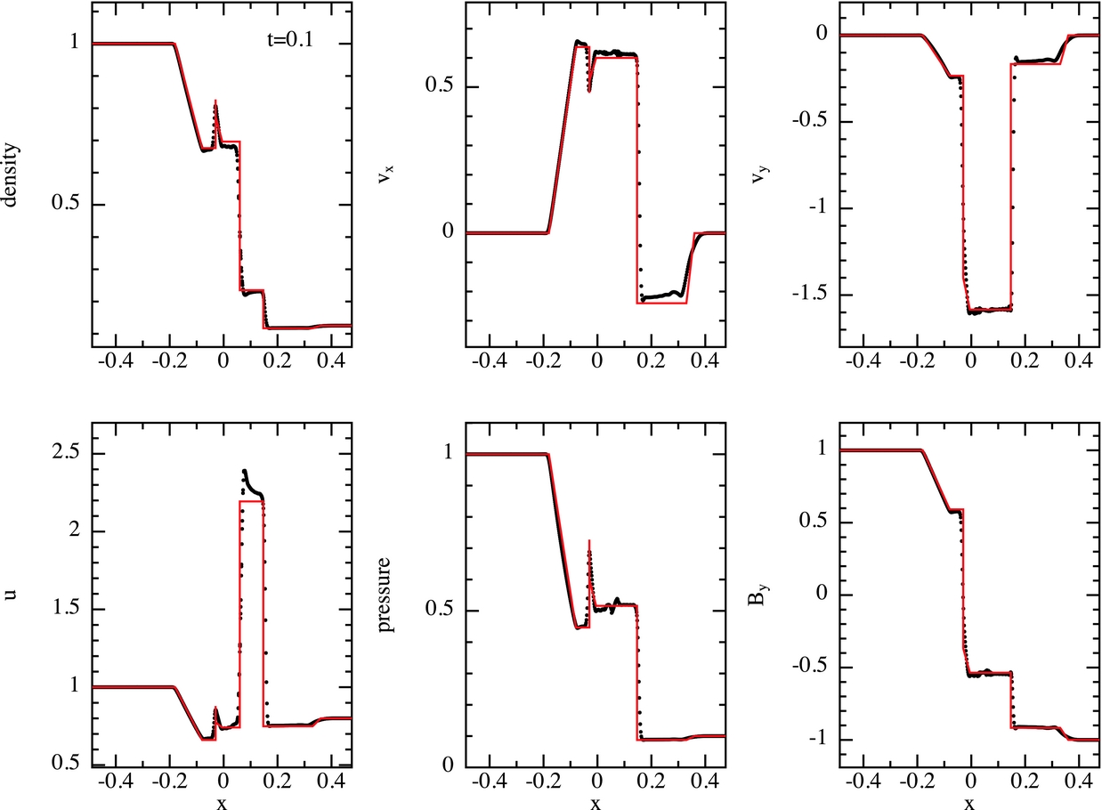
As in Figure 28 but using code defaults which give second-order convergence away from shocks. Some additional noise in the velocity field is visible, while otherwise the solutions are similar.
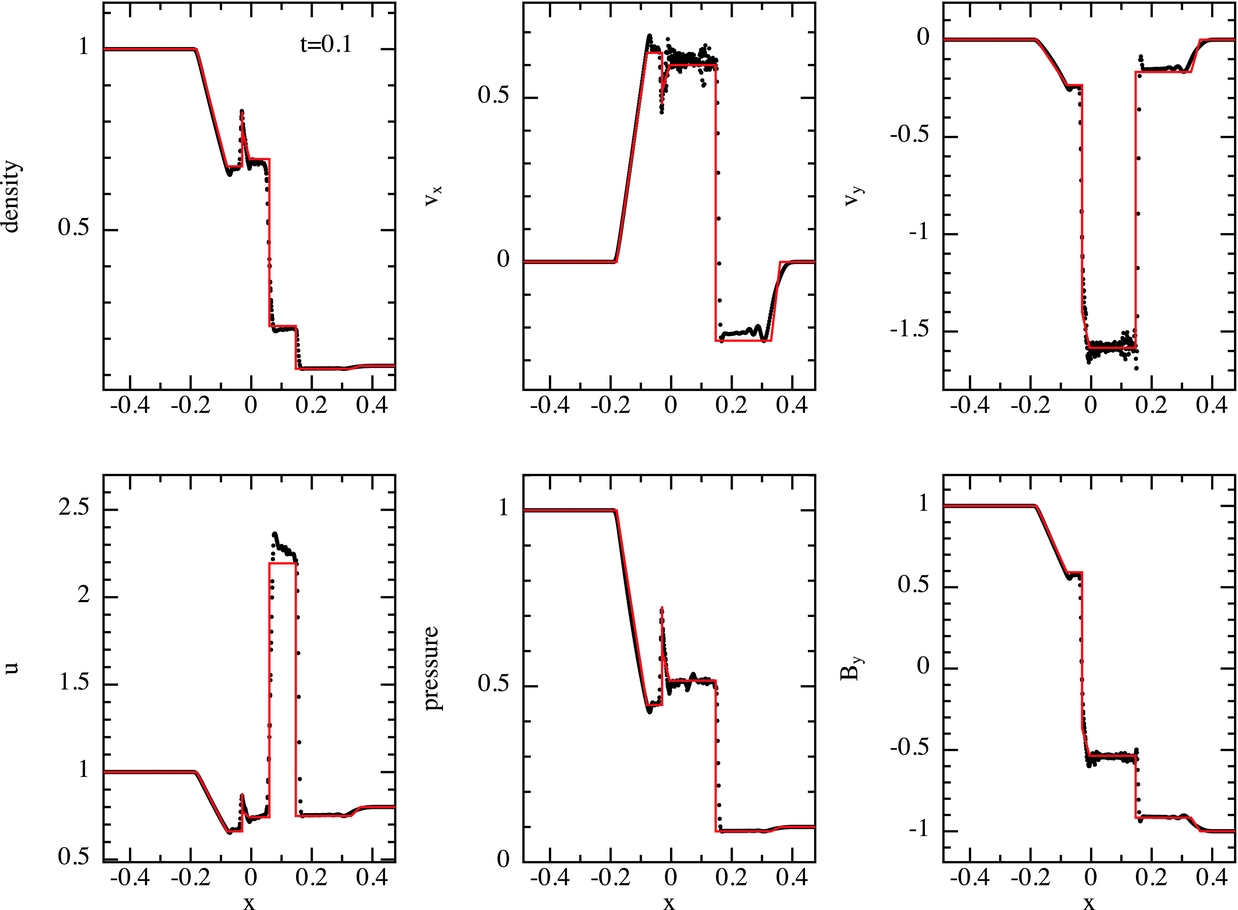
Figure 30 shows the result of the ‘seven-discontinuity’ test from Ryu & Jones (Reference Ryu and Jones1995). This test is particularly sensitive to over-dissipation by resistivity given the sharp jumps in the transverse magnetic and velocity fields. A reference solution with intermediate states taken from the corresponding table in Ryu & Jones (Reference Ryu and Jones1995) is shown by the red lines for comparison. Here the boundary particles are moved with a fixed velocity in the x-direction. The largest deviation from the reference solution is in the v y component, mainly due to the over-dissipation of the small spikes, with  ${\cal L}_1 = 0.02$ and ${\cal L}_2 = 0.07$ at this resolution. The remaining ${\cal L}_2$ errors are within 3% of the reference solution, while the ${\cal L}_1$ norms are smaller than 0.9% in all other variables.
Results of the seven-discontinuity MHD shock tube test 2a from Ryu & Jones (Reference Ryu and Jones1995) in 3D, showing projection of all particles (black dots) compared to the reference solution (red line). The problem is set up with  $[\rho , P, v_{x}, v_{y}, v_{z}, B_{x}, B_{y}, B_{z}] = [1.08,0.95,1.2,0.01,0.5,2/\sqrt{4\pi },3.6/\sqrt{4\pi },2/\sqrt{4\pi }]$ for x ⩽ 0 and $[\rho , P, v_{x}, v_{y}, v_{z}, B_{x}, B_{y}, B_{z}] = [1,1,0,0,0,2/\sqrt{4\pi },4/\sqrt{4\pi },2/\sqrt{4\pi }]$ for x > 0 with γ = 5/3. The density contrast is initialised using equal mass particles placed on a close packed lattice with 379 × 24 × 24 particles initially in x ∈ [− 0.5, 0] and 238 × 12 × 12 particles initially in x ∈ [0, 0.5].
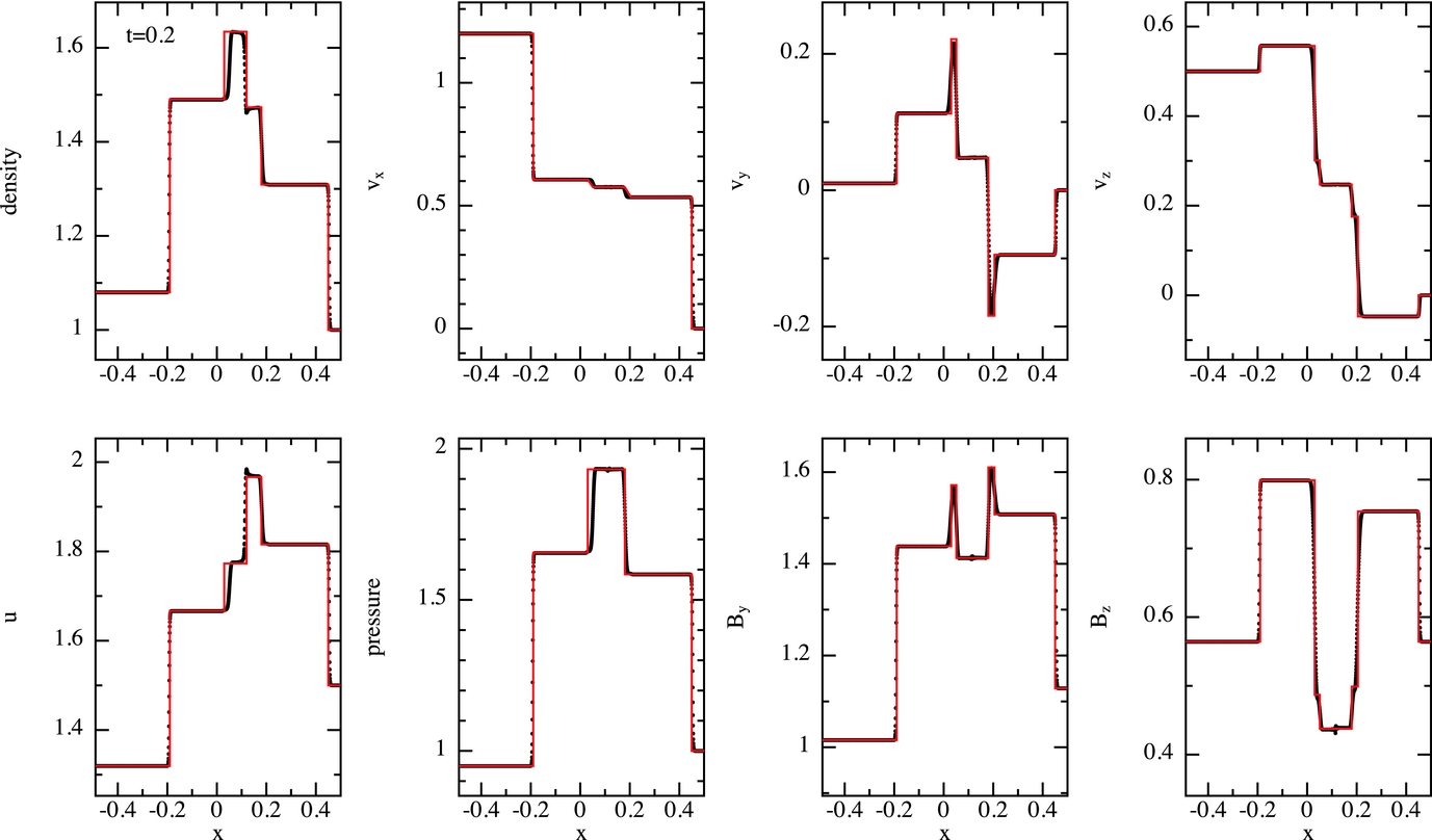
Finally, Figure 31 shows the results of shock tube 1a from Ryu & Jones (Reference Ryu and Jones1995). This test is interesting because it has historically proven to be a difficult test for SPMHD codes in more than 1D. In particular, to obtain reasonable results on this problem, Price & Monaghan (Reference Price and Monaghan2005) had to employ both an explicit shear viscosity term and a large neighbour number. Even then the jumps were found to show significant deviation from the analytic solution (see figure 10 in Price & Monaghan Reference Price and Monaghan2005). We did find that using h fac = 1.2 significantly improved the results of this test compared to our default h fac = 1.0 for the quintic kernel. Likewise, we found the results with the cubic spline kernel could be noisy. However, Figure 31 demonstrates that with only this change to the default code parameters, we can obtain results with  ${\cal L}_1$ errors of better than 4.4% in v y and less than 0.9% in all other variables at this resolution. The bottom left panel shows the errors induced in B x, with the largest error ( ${\cal L}_\infty$) only 0.6%. This is a substantial improvement over the 2D results shown in Price & Monaghan (Reference Price and Monaghan2005).
Results of the MHD shock tube test 1a from Ryu & Jones (Reference Ryu and Jones1995) in 3D, showing projection of all particles (black dots) compared to the reference solution (red line). The problem is set up with  $[\rho , P, v_{x}, v_{y}, v_{z}, B_{x}, B_{y}, B_{z}] = [1.0,20.0,10,0,0,5/\sqrt{4\pi },5/\sqrt{4\pi },0]$ for x ⩽ 0 and $[\rho , P, v_{x}, v_{y}, v_{z}, B_{x}, B_{y}, B_{z}] = [1,1,-10,0,0,5/\sqrt{4\pi },5/\sqrt{4\pi },0]$ for x > 0 with γ = 5/3. We show results using 652 × 12 × 12 particles. This has historically proven difficult for SPMHD codes. We find ${\cal L}_1$ within 1% of the reference solution except in v y (5%).
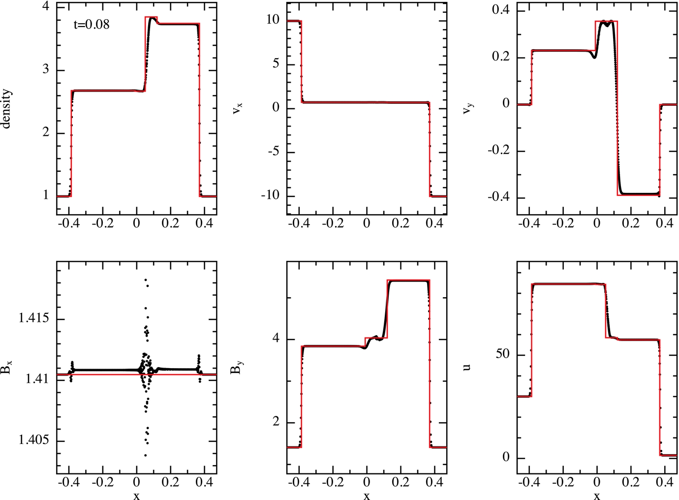
5.6.3. Orszag–Tang vortex
The Orszag–Tang vortex (Orszag & Tang Reference Orszag and Tang1979; Dahlburg & Picone Reference Dahlburg and Picone1989; Picone & Dahlburg Reference Picone and Dahlburg1991) has been used widely to test astrophysical MHD codes (e.g. Stone et al. Reference Stone, Hawley, Evans and Norman1992; Ryu, Jones, & Frank Reference Ryu, Jones and Frank1995; Dai & Woodward Reference Dai and Woodward1998; Tóth Reference Tóth2000; Londrillo & Del Zanna Reference Londrillo and Del Zanna2000). Similar to our hydrodynamic tests, we perform a 3D version of the original 2D test problem, similar to the ‘thin box’ setup used by Dolag & Stasyszyn (Reference Dolag and Stasyszyn2009). Earlier results on this test with 2D SPMHD can be found in Price & Monaghan (Reference Price and Monaghan2005), Rosswog & Price (Reference Rosswog and Price2007), Tricco & Price (Reference Tricco and Price2012, Reference Tricco and Price2013), Tricco et al. (Reference Tricco, Price and Bate2016a), and Hopkins & Raives (Reference Hopkins and Raives2016), and in 3D by Dolag & Stasyszyn (Reference Dolag and Stasyszyn2009) and Price (Reference Price2010).
The setup is a uniform density, periodic box x, y ∈ [− 0.5, 0.5] with boundary in the z direction set to  $\pm 2\sqrt{6}/n_x$, where n x is the initial number of particles in x, in order to setup the 2D problem in 3D (c.f. Section 5.1.4). We use an initial plasma β0 = 10/3, initial Mach number $\mathcal {M}_{0} = v_{0}/c_{\rm s, 0} = 1$, initial velocity field [v x, v y, v z] = [− v 0sin(2πy′), v 0sin(2πx′), 0], and magnetic field [B x, B y, B z] = [− B 0sin(2πy′), B 0sin(4πx′), 0], where v 0 = 1,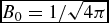 $B_{0} = 1/\sqrt{4\pi }$, x′ ≡ x − x min, and y′ ≡ y − y min; giving $P_{0} = \frac{1}{2} B_{0}^{2} \beta _{0} \approx 0.133$ and $\rho _{0} = \gamma P_{0} \mathcal {M}_{0} \approx 0.221$. We use an adiabatic EOS with γ = 5/3.
Figure 32 shows the results at t = 0.5 (top row) and at t = 1 (bottom) at resolutions of n x = 128, 256, and 512 particles (left to right). At t = 0.5, the main noticeable change as the resolution is increased is that the shocks become more well defined, as does the dense filament consisting of material trapped in the reconnecting layer of magnetic field in the centre of the domain. This current sheet eventually becomes unstable to the tearing mode instability (e.g. Furth, Killeen, & Rosenbluth Reference Furth, Killeen and Rosenbluth1963; Syrovatskii Reference Syrovatskii1981; Priest Reference Priest1985), seen by the development of small magnetic islands or ‘beads’ at t = 1 at high resolution (bottom right panel; c.f. Politano, Pouquet, & Sulem Reference Politano, Pouquet and Sulem1989). The appearance of these islands occurs only at high resolution and when the numerical dissipation is small [compare to the results using Euler potentials in 2D shown in Figure 13 of Tricco & Price (Reference Tricco and Price2012)], indicating that our implementation of artificial resistivity (Section 2.10.6) and divergence cleaning (Section 2.10.2) are effective in limiting the numerical dissipation.
Density in a z = 0 cross section of the Orszag-Tang vortex test performed in 3D. Results are shown at t = 0.5 (top) and t = 1 (bottom) at a resolution of 128 × 148 × 12, 256 × 296 × 12 and 512 × 590 × 12 particles (left to right). Compare e.g. to Figure 4 in Dai & Woodward (Reference Dai and Woodward1994b) or Figure 22 in Stone et al. (Reference Stone, Gardiner, Teuben, Hawley and Simon2008), while improvements in the SPMHD method over the last decade can be seen by comparing to Figure 14 in Price & Monaghan (Reference Price and Monaghan2005).
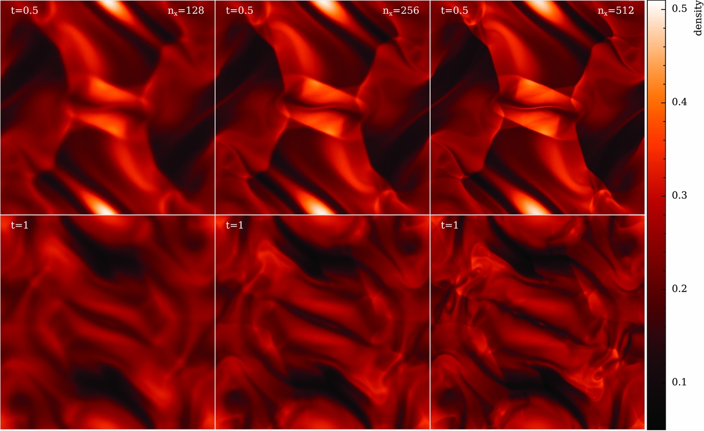
One other feature worth noting is that the slight ‘ringing’ behind the shock fronts visible in the results of Price & Monaghan (Reference Price and Monaghan2005) is absent from the low resolution calculation. This is because the Cullen & Dehnen (Reference Cullen and Dehnen2010) viscosity switch does a better job of detecting and responding to the shock compared to the previous Morris & Monaghan (Reference Morris and Monaghan1997)-style switch used in that paper. It is also worth noting that the results on this test, in particular, the coherence of the shocks, are noticeably worse without artificial resistivity, indicating that a small amount of dissipation in the magnetic field is necessary to capture MHD shocks correctly in SPMHD (c.f. Price & Monaghan Reference Price and Monaghan2004a, Reference Price and Monaghan2005; Tricco & Price Reference Tricco and Price2012).
Figure 33 shows horizontal slices of the pressure at t = 0.5, showing cuts along y = 0.3125 (top) and y = 0.4277 (bottom) following (e.g.) Londrillo & Del Zanna (Reference Londrillo and Del Zanna2000) and Stone et al. (Reference Stone, Gardiner, Teuben, Hawley and Simon2008). The main difference at higher resolution is that the shocks become sharper and more well defined. Most of the smooth flow regions are converged with n x = 256 (i.e. the red and black lines are indistinguishable), but the parts of the flow where dissipation is important are can be seen to converge more slowly. This is expected.
Horizontal slices of pressure shown at t=0.5 in the Orszag–Tang vortex test. We show cuts along y = 0.3125 (top) and y = 0.4277 (bottom) in the z = 0 plane for three different numerical resolutions (see legend).
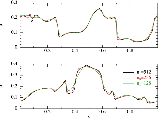
5.6.4. MHD rotor problem
Balsara & Spicer (Reference Balsara and Spicer1999) introduced the ‘MHD rotor problem’ to test the propagation of rotational discontinuities. Our setup follows Tóth (Reference Tóth2000)’s ‘first rotor problem’ as used by Price & Monaghan (Reference Price and Monaghan2005), except that we perform the test in 3D. A rotating dense disc of material with ρ = 10 is set up with cylindrical radius R = 0.1, surrounded by a uniform periodic box [x, y] ∈ [− 0.5, 0.5] with the z boundary set to  $[-\sqrt{6}/(2n_{x}),\sqrt{6}/(2n_{x})]$, or 12 particle spacings on a close packed lattice. The surrounding medium has density ρ = 1. Initial velocities are v x, 0 = −v 0(y − y 0)/r and v y, 0 = v 0(x − x 0)/r for r < R, where v 0 = 2 and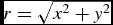 $r = \sqrt{x^{2} + y^{2}}$. The initial pressure P = 1 everywhere while the initial magnetic field is given by $[B_{x}, B_{y}, B_{z}] = [5/\sqrt{4\pi }, 0, 0]$ with γ = 1.4. We set up the initial density contrast unsmoothed, as in Price & Monaghan (Reference Price and Monaghan2005), by setting up two uniform lattices of particles masked to the initial cylinder, with the particle spacing adjusted inside the cylinder by the inverse cube root of the density contrast. At a resolution of n x = 256 particles for the closepacked lattice, this procedure uses 1 145 392 particles, equivalent to a 2D resolution of ~3002, inbetween the 2002 results shown in Tóth (Reference Tóth2000) and Price & Monaghan (Reference Price and Monaghan2005) and the 4002 used in Stone et al. (Reference Stone, Gardiner, Teuben, Hawley and Simon2008).
Figure 34 presents the results of this test, showing 30 contours in density, pressure, Mach number, and magnetic pressure using limits identical to those given in Tóth (Reference Tóth2000). The symmetry of the solution is preserved by the numerical scheme and the discontinuities are sharp, as discussed in Stone et al. (Reference Stone, Gardiner, Teuben, Hawley and Simon2008). The contours we obtain with Phantom are noticeably less noisy than the earlier SPMHD results given in Price & Monaghan (Reference Price and Monaghan2005), a result of the improvement in the treatment of dissipation and divergence errors in SPMHD since then (c.f. Section 2.10; see also recent results in Tricco et al. Reference Tricco, Price and Bate2016a).
Density, pressure, Mach number, and magnetic pressure shown in a z = 0 cross section at t = 0.15 in the 3D MHD rotor problem, using n x = 256, equivalent to ~3002 resolution elements in 2D. The plots show 30 contours with limits identical to those given by Tóth (Reference Tóth2000); 0.483 < ρ < 12.95, 0.0202 < P < 2.008, 0 < |v|/c s < 1.09, and  $0 < \frac{1}{2} B^{2} < 2.642$.
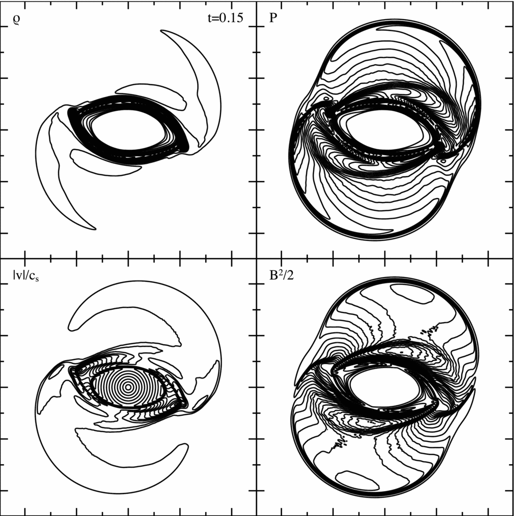
5.6.5. Current loop advection
The current loop advection test was introduced by Gardiner & Stone (Reference Gardiner and Stone2005, Reference Gardiner and Stone2008), and regarded by Stone et al. (Reference Stone, Gardiner, Teuben, Hawley and Simon2008) as the most discerning of their code tests. We perform this test in 3D, as in the ‘first 3D test’ from Stone et al. (Reference Stone, Gardiner, Teuben, Hawley and Simon2008) by using a thin 3D box with non-zero v z. The field setup is with a vector potential A z = A 0(R − r) for r < R, giving B x = −A 0y/r, B y = A 0x/r and B z = 0, where 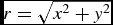 $r = \sqrt{x^{2} + y^{2}}$, R = 0.3 and we use A 0 = 10−3, ρ0 = 1, P 0 = 1, and an adiabatic EOS with γ = 5/3. We use a domain $[x, y, z] \in [-1:1,-0.5:0.5,-\sqrt{6}/(2n_{x}):\sqrt{6}/(2n_{x})]$ with $[v_{x}, v_{y}, v_{z}] = [2, 1, 0.1 /\sqrt{5}]$. The test is difficult mainly because of the cusp in the vector potential gradient at r = R leading to a cylindrical current sheet at this radius. The challenge is to advect this infinite current without change (in numerical codes the current is finite but with a magnitude that increases with resolution). We choose the resolution to be comparable to Stone et al. (Reference Stone, Gardiner, Teuben, Hawley and Simon2008).
For SPMHD, this is mainly a test of the shock dissipation and divergence cleaning terms, since in the absence of these terms the advection can be computed to machine precision [c.f. 2D results shown in Rosswog & Price (Reference Rosswog and Price2007) and Figure 11 of Price (Reference Price2012a), shown after one thousand crossings of the computational domain]. Figure 35 shows the results of this test in Phantom with 128 × 74 × 12 particles after two box crossings, computed with all dissipation and divergence cleaning terms switched on, precisely as in the previous tests including the shock tubes (Sections 5.6.2–5.6.4). Importantly, our implementation of artificial resistivity (Section 2.10.6) guarantees that the dissipation is identically zero when there is no relative velocity between the particles, meaning that simple advection of the current loop is not affected by numerical resistivity. However, the problem remains sensitive to the divergence cleaning (Section 2.10.2), in particular to any spurious divergence of  ${\bm B}$ that is measured by the SPMHD divergence operator, (174). For this reason, the results using the quintic kernel, (19), are substantially better than those using the cubic spline, because the initial measurement of $\nabla \cdot {\bm B}$ is smaller and so the evolution is less affected by the divergence cleaning.
Magnitude of the current density  $\vert \nabla \times {\bm B} \vert$ in the current loop advection test performed in 3D, showing comparing the initial conditions (top) to the result after two (middle) and five (bottom) crossings of the box, using 128 × 74 × 12 particles. Full dissipation, shock capturing, and divergence cleaning terms were applied for this test, without which the advection is exact to machine precision. The advection is affected mainly by the divergence cleaning acting on the outer (infinite) current sheet.
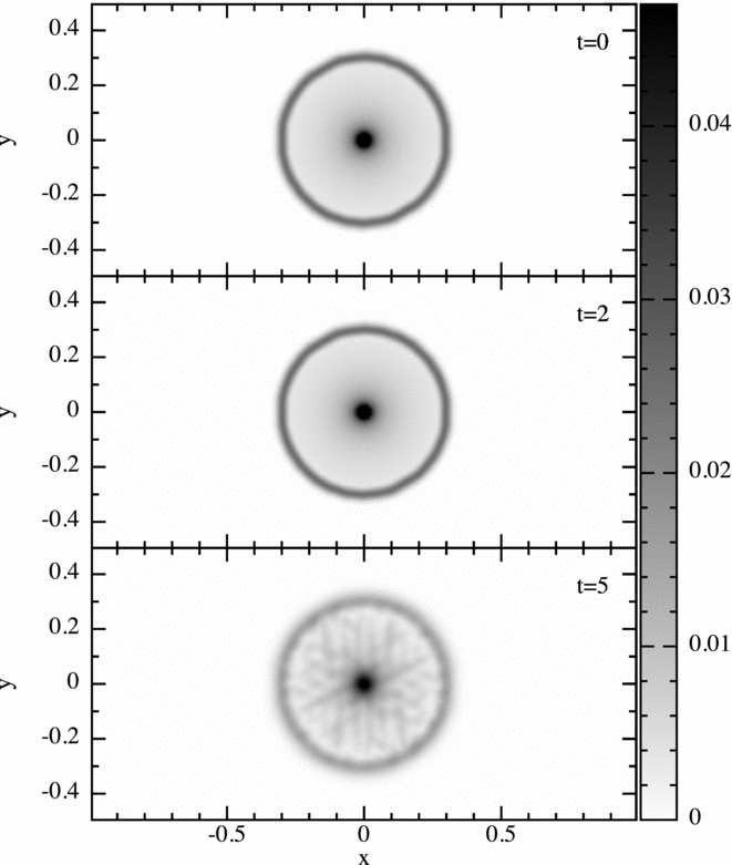
5.6.6. MHD blast wave
The MHD blast wave problem consists of an over-pressurised central region that expands preferentially along the strong magnetic field lines. Our setup uses the 3D initial conditions of Stone et al. (Reference Stone, Gardiner, Teuben, Hawley and Simon2008), which follows from the work of Londrillo & Del Zanna (Reference Londrillo and Del Zanna2000) and Balsara & Spicer (Reference Balsara and Spicer1999). For a recent application of SPMHD to this problem, see Tricco & Price (Reference Tricco and Price2012) and Tricco et al. (Reference Tricco, Price and Bate2016a). Set in a periodic box [x, y, z] ∈ [− 0.5, 0.5], the fluid has uniform ρ = 1 and  ${\bm B} = [10 / \sqrt{2}, 0, 10 / \sqrt{2}]$. The pressure is set to P = 1, using γ = 1.4, except for a region in the centre of radius R = 0.125 which has its pressure increased to P = 100. This yields initial plasma beta β = 2 inside the blast and β = 0.02 outside. The particles are arranged on a close-packed triangular lattice using n x = 256.
Figure 36 shows slices through y = 0 of density, pressure, magnetic energy density, and kinetic energy density, which may be directly compared to results in Gardiner & Stone (Reference Gardiner and Stone2008). The shock positions and overall structure of the blast wave in all four variables show excellent agreement with the results shown in their paper. The main difference is that their solution appears less smoothed, suggesting that the overall numerical dissipation is lower in Athena.
Slices through y = 0 for the MHD blast wave problem showing density (top left), gas pressure (top right), magnetic energy density (bottom left), and kinetic energy density (bottom right). The plot limits are ρ ∈ [0.19, 2.98], P ∈ [1, 42.4], [25.2, 64.9] for the magnetic energy density and [0, 33.1] for the kinetic energy density. These are directly comparable to Figure 8 in Gardiner & Stone (Reference Gardiner and Stone2008).
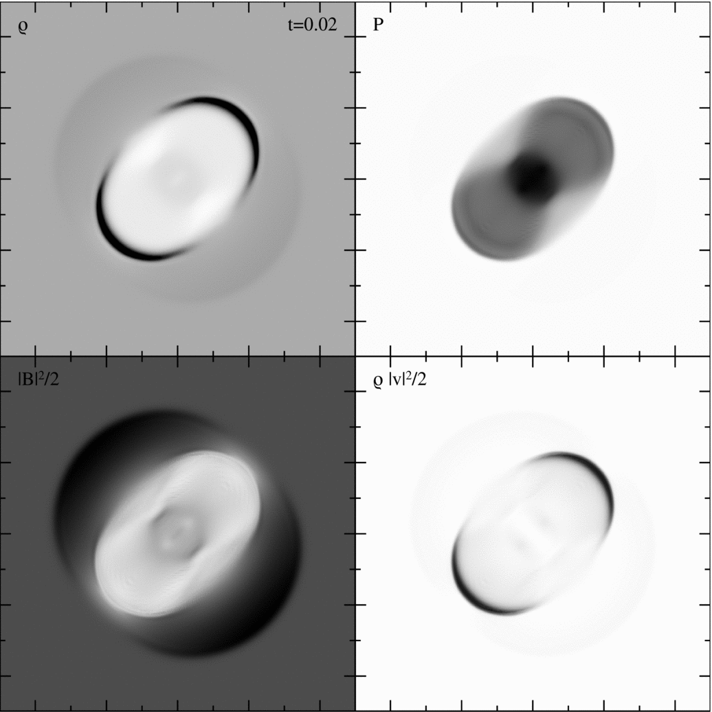
5.6.7. Balsara–Kim supernova-driven turbulence
We reproduce the ‘test problem’ of Balsara & Kim (Reference Balsara and Kim2004) (hereafter BK04) modelling supernova-driven turbulence in the interstellar medium. BK04 used this test to argue strongly against the use of divergence cleaning for problems involving strong shocks. Specifically, they compared three different divergence cleaning schemes against a constrained transport method, finding that divergence cleaning was unusable for such problems, with all three divergence cleaning schemes producing strong temporal fluctuations in magnetic energy during the growth phase of the supernova-driven dynamo. The problems were attributed to issues with the non-locality of divergence cleaning.
We follow the setup in BK04 as closely as possible, but several issues make a direct comparison difficult. Chief among these is their use of a physical ISM cooling prescription. We implement a similar algorithm (Section 2.14), but our cooling prescription is not identical (e.g. our implementation includes live chemistry and thus the possibility for a cold phase of the ISM, which theirs does not). Second, they give the setup parameters for the problem in computational units, but the use of ISM cooling requires the physical units of the problem to be specified. Since these are not stated in their paper, one must guess the units by reading descriptions of the same problem in physical units given in Kim, Balsara, & Mac Low (Reference Kim, Balsara and Mac Low2001), Balsara et al. (Reference Balsara, Kim, Mac Low and Mathews2004), and Mac Low et al. (Reference Mac Low, Balsara, Kim and de Avillez2005).
We set up the problem as follows. Particles are initialised on a close-packed lattice in a periodic box with x, y, z ∈ [− 0.1, 0.1], with ρ = 1 and the initial thermal pressure set to P = 0.3 (all in code units, as specified in BK04). We infer a length unit of kpc since this is described as a ‘200 pc3 box’ in their other papers. We employ an adiabatic EOS with γ = 5/3 and turn on interstellar cooling and chemistry in the code with default initial abundances (i.e. atomic Hydrogen everywhere). We choose the mass unit such that a density of 2.3 × 10⁻²³ g cm−3, as described in Kim et al. (Reference Kim, Balsara and Mac Low2001), corresponds to ρ = 1 in code units as described in BK04. Finally, we set the time unit such that G = 1 in code units (a common choice, even though gravity is not involved in the problem). We compute the problem using resolutions of 64 × 74 × 78 particles and 128 × 148 × 156 particles.
Supernovae are injected into the simulation every 0.00125 in code units at the positions listed in Table 1 of BK04. We infer this to correspond to the ‘12 × Galactic’ rate described in Balsara et al. (Reference Balsara, Kim, Mac Low and Mathews2004), i.e. 12 times faster than 1 per 1.26 Myr. We inject supernovae following the description in BK04 by setting the pressure to P = 13649.6 on particles within a distance of 0.005 code units from the injection site (corresponding to a radius of 5 pc in physical units). Our choice of units means that this corresponds to an energy injection within a few percent of 1051 ergs in physical units, corresponding to the description given in their other papers. However, this is only true if the density equals the initial value, since BK04 specify pressure rather than the energy. We follow the description in BK04 (i.e. we set the pressure), even though this gives an energy not equal to 1051 ergs if injected in a low or high density part of the computational domain.
The initial magnetic field is uniform in the x-direction with B x = 0.056117, as stated in BK04. We could not reconcile this with the magnetic energy plotted in their paper, which show an initial magnetic energy of 10−6. Nor could we reconcile this with the statement in Balsara et al. (Reference Balsara, Kim, Mac Low and Mathews2004) that ‘the magnetic energy is 10−6 times smaller than the thermal energy’. So any comparison is approximate. Nevertheless, BK04 state that the problems caused by divergence cleaning are not dependent on specific details of the implementation.
Figure 37 shows the evolution of the column density in the lowest resolution calculation using 64 × 74 × 78 particles. The combination of supernovae injection and cooling drives turbulence and significant structure in the density field.
Balsara–Kim supernova-driven turbulence, showing column density at three different times at a resolution of 64 × 74 × 78 particles. Supernovae are injected every 0.00125 in code units, leading to a series of interacting blast waves. Interstellar chemistry and cooling is turned on, producing a dense filaments in a turbulent interstellar medium.
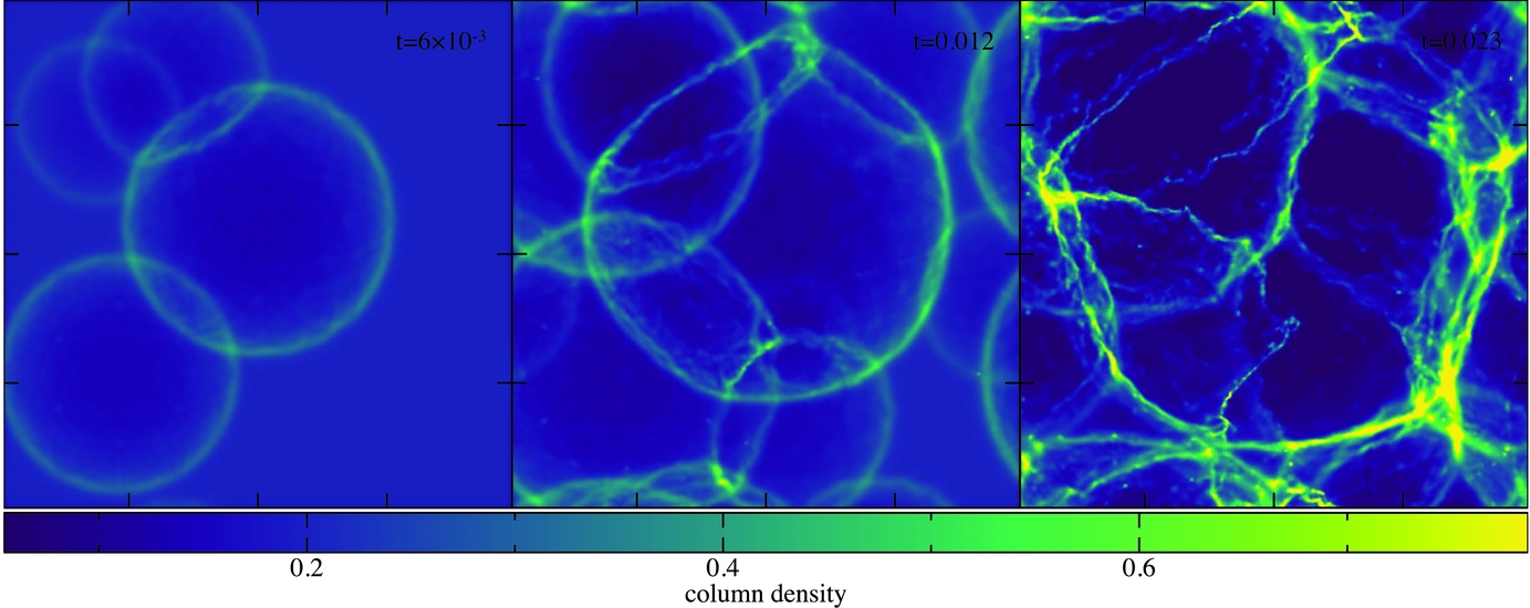
To specifically address the issues found by BK04, Figure 38 shows a cross-section slice of the magnetic pressure at a time similar to the one shown in Figure 3 of BK04 (they do not indicate which slice they plotted, we chose z = 0.0936). The magnetic pressure in the interior of the supernovae shells is smooth, and does not display any of the large-scale artefacts of the type found in their paper.
Cross-section slice of magnetic pressure at t = 0.006 in the Balsara–Kim supernova-driven turbulence test using 128 × 148 × 156 particles. No large-scale artefacts in magnetic energy are visible, indicating that the simulation is not corrupted by divergence cleaning.
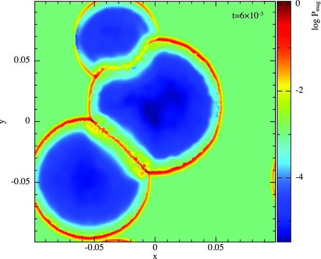
Figure 39 shows the time evolution of the magnetic energy in the low-resolution calculation. The magnetic energy rises monotonically up to t ≈ 0.02 before the magnetic energy saturates, similar to what was found by BK04 for their staggered mesh/constrained transport scheme (compare with Figure 2 in their paper). There are no large temporal fluctuations in the magnetic energy of the kind they report for their divergence cleaning methods.
Magnetic energy as a function of time in the Balsara–Kim supernova-driven turbulence problem. The magnetic energy increases monotonically by approximately an order of magnitude before reaching its saturation value at t ≈ 0.02. There are no spurious spikes in magnetic energy caused by divergence cleaning, in contrast to what was found by Balsara & Kim (Reference Balsara and Kim2004).
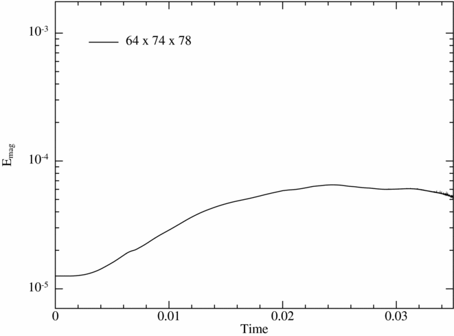
In summary, the results we obtain for the magnetic field energy and structure within supernova-driven turbulence in the interstellar medium match closest the constrained transport result of BK04. There is no evidence that our simulations experience the numerical issues encountered by BK04 with their divergence cleaning schemes, suggesting that the problems they reported are primarily code dependent rather than being fundamental. The most probable reason our results are of the same quality as BK04’s constrained transport result is our use of constrained divergence cleaning, which guarantees that energy removed from the magnetic field is negative definite. A follow-up study to examine this in more depth would be worthwhile. For our present purposes, we can conclude that our divergence cleaning algorithm is sufficiently robust—even in ‘real-world’ problems—to be useful in practice (see also Section 6.3).
5.7. Non-ideal MHD
The following tests demonstrate the non-ideal MHD algorithms (Section 2.11). We adopt periodic boundary conditions for both tests, initialising the particles on a close-packed lattice with an isothermal EOS, P = c 2sρ, and using the C 4 Wendland kernel.
5.7.1. Wave damping test
To test ambipolar diffusion in the strong coupling approximation, we follow the evolution of decaying Alfvén waves, as done in (e.g.) Choi, Kim, & Wiita (Reference Choi, Kim and Wiita2009) and Wurster et al. (Reference Wurster, Price and Ayliffe2014).
In arbitrary units, the initial conditions are a box of size  $L_{\rm x} \times \frac{\sqrt{3}}{2}L_{\rm x} \times \frac{\sqrt{6}}{2}L_{\rm x}$ with L x = 1, a density of ρ = 1, magnetic field of $\bm {B} = B_0\hat{\bm {x}}$ with B 0 = 1, sound speed of c s = 1, and velocity of $\bm {v} = v_0\sin (kx)\hat{\bm {z}}$, where k = 2π/L x is the wave number, and v 0 = 0.01v A, where v A is the Alfvén velocity. We adopt an ambipolar diffusion coefficient of ηAD = 0.01v 2A. All artificial dissipation terms are turned off. We use n x = 128 particles.
The solution to the dispersion relation for Alfvén waves (Balsara Reference Balsara1996) is
 $$\begin{equation}
\omega ^2 + \eta _{\rm AD}k^2 \omega i- v_{\rm A}^2k^2 = 0,
\end{equation}$$
$$\begin{equation}
\omega ^2 + \eta _{\rm AD}k^2 \omega i- v_{\rm A}^2k^2 = 0,
\end{equation}$$
where ω = ωR + ωIi is the complex angular frequency of the wave, giving a damped oscillation in the form
 $$\begin{equation}
h(t) = h_0 \left| \sin \left(\omega _{\rm R}t\right)\right|\text{e}^{\omega _{\rm I}t}.
\end{equation}$$
$$\begin{equation}
h(t) = h_0 \left| \sin \left(\omega _{\rm R}t\right)\right|\text{e}^{\omega _{\rm I}t}.
\end{equation}$$
In our test, h(t) corresponds the root mean square of the magnetic field in the z-direction, < B 2z > 1/2, and  $h_0 = v_0 B_0 / (v_{\rm A} \sqrt{2})$.
Figure 40 shows the time evolution of < B 2z > 1/2 to t = 5 for both the numerical results (blue line) and the analytic solution (red line). At the end of the test, the  ${\cal L}_2$ error is 7.5 × 10⁻⁵ (evaluated at intervals of dt = 0.01), demonstrating close agreement between the numerical and analytical results.
Wave damping test showing the decay of Alfvén waves in the presence of ambipolar diffusion, using the coefficient ηAD = 0.01v 2A. The  ${\cal L}_2$ error between the analytic and numerical solution is 7.5 × 10⁻⁵.
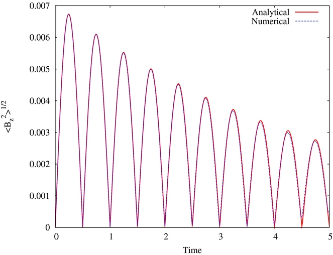
Given that, by design, there is motion of the particles and that we have excluded artificial dissipation, the particles tend to ‘break’ from the initial lattice. For both the M 6 quintic kernel and the C 4 Wendland kernel on a cubic lattice, the particles fall off the lattice at t ≈ 0.75. Prior to this, however, the  ${\cal L}_2$ error is smaller than that calculated using the C 4 Wendland kernel and a close-packed lattice, thus there is a trade off between accuracy and long-term stability.
5.7.2. Standing shock
To test the Hall effect, we compare our solutions against the 1D isothermal steady-state equations for the strong Hall effect regime. The numerical solution to this problem is given in Falle (Reference Falle2003) and O’Sullivan & Downes (Reference O’Sullivan and Downes2006), and also summarised in Appendix C1.2 of Wurster et al. (Reference Wurster, Price and Bate2016).
The left- and right-hand side of the shock are initialised with (ρ0, v x, 0, v y, 0, v z, 0, B x, 0, B y, 0, B z, 0) = (1.7942, −0.9759, −0.6561, 0.0, 1.0, 1.74885, 0.0) and (1.0, −1.751, 0.0, 0.0, 1.0, 0.6, 0.0), respectively, with the discontinuity at x = 0. We use boundary particles at the x-boundary, superseding the periodicity in this direction. To replicate inflowing boundary conditions in the x-direction, when required, the initial domain of interest x l < x < x r is automatically adjusted to x′l < x < x′r, where x′r = xr − v 0t max, where t max is the end time of the simulation. Note that for inflowing conditions, x r and v 0 will have opposite signs. Thus, at the end of the simulation, the entire range of interest will still be populated with particles.
The non-ideal MHD coefficients are ηOR = 1.12 × 10⁻¹², ηHE = −3.53 × 10⁻²B, and ηAD = 7.83 × 10 − 3v 2A. We include all artificial dissipation terms using their default settings. We initialise 512 × 14 × 15 particles in x < 0 and 781 × 12 × 12 particles in x ⩾ 0, with the domain extending from xl = x′l = −2 to x r = 2 with x′r = 3.75.
Figure 41 shows v x and B y for both the numerical and analytical results, which agree to within 3% at any given position.
Hall-dominated standing shock using ηOR = 1.12 × 10⁻¹², ηHE = −3.53 × 10⁻²B, and ηAD = 7.83 × 10 − 3v 2A. The numerical and analytical results agree to within 3% everywhere.
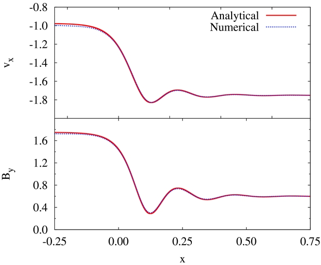
On the left-hand side of the shock interface, the numerical results are lower than the analytical solution because of the artificial dissipation terms, which are required to properly model a shock. These results do not depend on either the kernel choice or the initial particle lattice configuration.
5.8. Self-gravity
5.8.1. Polytrope
The simplest test of self-gravity is to model a spherical polytrope in hydrostatic equilibrum. Similar tests have been shown for SPH codes dating back to the original papers of Gingold & Monaghan (Reference Gingold and Monaghan1977, Reference Gingold and Monaghan1978, Reference Gingold and Monaghan1980). Modern calculations have used these simple models in more complex applications, ranging from common envelope evolution (Iaconi et al. Reference Iaconi, Reichardt, Staff, De Marco, Passy, Price, Wurster and Herwig2017) to tidal disruption events (Coughlin & Nixon Reference Coughlin and Nixon2015; Coughlin et al. Reference Coughlin, Nixon, Begelman and Armitage2016b, Reference Coughlin, Armitage, Nixon and Begelman2016a; Bonnerot et al. Reference Bonnerot, Rossi, Lodato and Price2016, Reference Bonnerot, Price, Lodato and Rossi2017).
The EOS is P = Kργ, with γ = 1 + 1/n where n is the polytropic index. The exact hydrostatic solution is given by
 $$\begin{equation}
\frac{\gamma K}{4\pi G\left(\gamma - 1\right) }\frac{\text{d}^2}{\text{d}r^2}\left(r\rho ^{\gamma -1}\right) + r\rho = 0.
\end{equation}$$
$$\begin{equation}
\frac{\gamma K}{4\pi G\left(\gamma - 1\right) }\frac{\text{d}^2}{\text{d}r^2}\left(r\rho ^{\gamma -1}\right) + r\rho = 0.
\end{equation}$$
Our initial setup uses a solution scaled to a radius R = 1, for a polytropic index of n = 3/2, corresponding to γ = 5/3, with K = 0.4244. We solve (325) numerically. We place the particles initially on a hexagonal close-packed lattice, truncated to a radius of R = 1, which we then stretch map (see Section 3.2) such that the initial radial density profile matches the exact solution.
The relaxation time depends on the initial density profile and on how far the initial particle configuration is from equilibrium. Figure 42 shows the solution at t = 100 in code units. The polytrope relaxes within a few dynamical times, with only a slight rearrangement of the particles from the stretched lattice. The density profile at all times is equal to within 3% of the exact solution for r ⩽ 0.7 and the polytrope remains in hydrostatic equilibrium.
Polytrope static structure using 106 particles (black), compared to the exact solution (red), shown at t = 100.
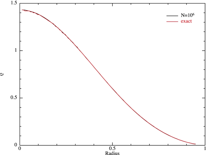
Once the static solution is obtained, we tested the energy conservation by giving the star a radial perturbation. That is, we applied a velocity perturbation of the form v r = 0.2r to the N ≈ 105 model, and evolved the polytrope for 100 time units. We turned off the artificial viscosity for this test. The total energy—including contributions from thermal, kinetic, and gravitational energy—remained conserved to within 3%.
5.8.2. Binary polytrope
Next, we placed two initially unrelaxed, identical polytropes, each with N = 104 particles in a circular orbit around each other with a separation of 6R and evolved for ~15 orbits (1 000 code units). Figure 43 demonstrates that the separation remains within 1% of the initial separation over 15 orbits, and that the orbital period remains constant. After the initial relaxation, total energy is conserved to within 0.06%.
y- and x-positions of the centre of mass of one star of a binary system (top and bottom, respectively). Each star is a polytrope with mass and radius of unity, and N = 104 particles; the initial separation is 6.0 in code units. After ~15 orbits, the separation remains within 1%, and the period remains constant within the given time resolution. The red line represents the analytical position with respect to time, and the black line represents the numerical position.
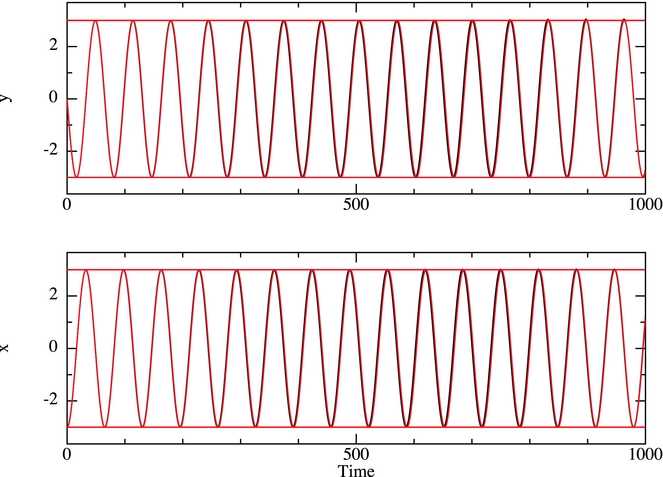
The stars are far enough apart that any tidal deformation as they orbit is insignificant. The final density profile of each star agrees with the expected profile within 3% for r ⩽ 0.7.
5.8.3. Evrard collapse
A more complex test, relevant especially for star formation, is the so-called ‘Evrard collapse’ (Evrard Reference Evrard1988) modelling the adiabatic collapse of a cold gas sphere. It has been used many times to test SPH codes with self-gravity, e.g. Hernquist & Katz (Reference Hernquist and Katz1989), Steinmetz & Mueller (Reference Steinmetz and Mueller1993), Thacker et al. (Reference Thacker, Tittley, Pearce, Couchman and Thomas2000), Escala et al. (Reference Escala, Larson, Coppi and Mardones2004), and many others.
Following the initial conditions of Evrard (Reference Evrard1988), we setup the particles initially in a sphere of radius R = 1 and mass M = 1, with density profile
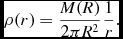 $$\begin{equation}
\rho (r) = \frac{M(R)}{2\pi R^2}\frac{1}{r}.
\end{equation}$$
$$\begin{equation}
\rho (r) = \frac{M(R)}{2\pi R^2}\frac{1}{r}.
\end{equation}$$
The density profile is created using the same stretch mapping method as for the polytrope (see Section 5.8.1). The sphere is initially isothermal, with the specific internal energy set to u = 0.05GM/R with an adiabatic index of γ = 5/3. The sphere initially undergoes gravitational collapse.
In the literature, the results of the Evrard collapse are typically normalised to a characteristic value. Here, we simply show the results in code units (Section 2.2.3), since these units already represent a normalised state. A distance unit of R = 1 and mass unit M(R) = 1 is adopted, with the time unit set such that G ≡ 1, where G is the gravitational constant.
Figure 44 shows the kinetic, thermal, total, and potential energies as a function of time, at four different numerical resolutions. The green line shows the reference solution, computed using a 1D piecewise parabolic method (PPM) code using 350 zones, which we transcribed from Figure 6 of Steinmetz & Mueller (Reference Steinmetz and Mueller1993).
Thermal, kinetic, total, and potential energies as a function of time during the Evrard collapse (Evrard Reference Evrard1988). Green lines are calculated using a 1D PPM code, taken from Figure 6 of Steinmetz & Mueller (Reference Steinmetz and Mueller1993), while remaining colours show SPH simulations of different resolutions. Both energy and time are given in code units, where R = M = G = 1.
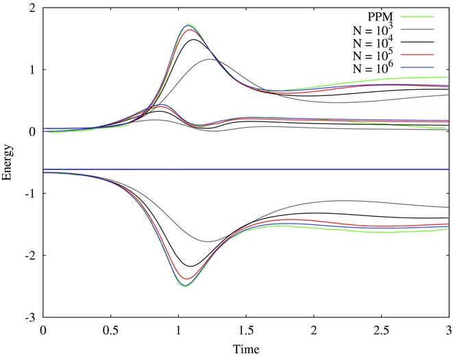
As the number of particles increases, the energies for t ≲ 1.5 converge to the results obtained from the PPM code. At t ≳ 2, the SPH results appear to converge to energies that differ slightly from the PPM code. Given that we are not able to perform a comparable convergence study with the PPM code, we are unable to assess whether or not this discrepancy is significant.
Figure 45 shows enclosed mass, density, thermal energy, and radial velocity as a function of radius at t = 0.77, where the SPH results may be compared to the PPM results presented by Steinmetz & Mueller (Reference Steinmetz and Mueller1993) shown with the red line in the figure. At this time, the outward propagating shock is at r ≈ 0.1, with the shock profile in agreement with the reference solution at high resolution.
Radial profile of the Evrard collapse (Evrard Reference Evrard1988) at t = 0.77, red lines are taken from Figure 7 of Steinmetz & Mueller (Reference Steinmetz and Mueller1993), with panels showing density (top) and radial velocity (bottom) as a function of (log) radius. All values are given in code units, where R = M = G = 1. The outward propagating shock at r ≈ 0.1 is sharper at high resolution.
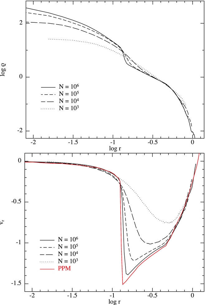
5.9. Dust–gas mixtures
The SPH algorithms used in Phantom for dust–gas mixtures have been extensively benchmarked in Laibe & Price (Reference Laibe and Price2012a, Reference Laibe and Price2012b) (for the two-fluid method) and in Price & Laibe (Reference Price and Laibe2015a) (for the one-fluid method; hereafter PL15). Here, we merely demonstrate that the implementation of these algorithms in Phantom gives satisfactory results on these tests. For recent applications of Phantom to more realistic problems involving dust/gas mixtures, see Dipierro et al. (Reference Dipierro, Price, Laibe, Hirsh and Cerioli2015, Reference Dipierro, Laibe, Price and Lodato2016), Ragusa et al. (Reference Ragusa, Dipierro, Lodato, Laibe and Price2017), and Tricco et al. (Reference Tricco, Price and Laibe2017).
5.9.1. Dustybox
Figure 46 shows the results of the dustybox problem (Monaghan & Kocharyan Reference Monaghan and Kocharyan1995; Paardekooper & Mellema Reference Paardekooper and Mellema2006; Laibe & Price Reference Laibe and Price2011). We setup a uniform, periodic box x, y, z ∈ [− 0.5, 0.5] with 32 × 36 × 39 gas particles set on a close-packed lattice and 32 × 36 × 39 dust particles also set on a close-packed lattice. The gas particles are initially at rest, while the dust is given a uniform velocity v x = 1 in the x-direction. We employ an isothermal EOS with c s = 1, uniform gas and dust densities of ρg = ρd = 1, using the cubic spline kernel for the SPH terms and the double-hump cubic spline kernel (Section 2.13.4) for the drag terms, following Laibe & Price (Reference Laibe and Price2012a).
Decay of kinetic energy as a function of time in the dustybox test, involving a uniformly translating mixture of gas and dust coupled by drag. Solid lines show the Phantom results for drag coefficients K = 0.01, 0.1, 1.0, 10, and 100 (top to bottom), which may be compared to the corresponding analytic solutions given by the dashed red lines.
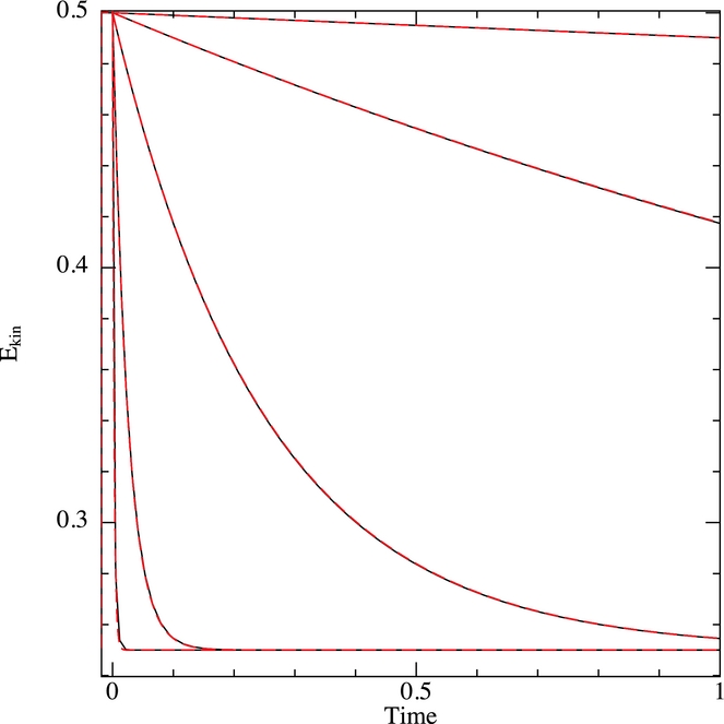
The red dashed lines in Figure 46 show the exact solution for kinetic energy as a function of time. For our chosen parameters, the barycentric velocity is v x = 0.5, giving v g(t) = 0.5[1 + Δv x(t)], v d(t) = 0.5[1 − Δv x(t)], where Δv x(t) = exp(− 2Kt) (Laibe & Price Reference Laibe and Price2011) and the red lines show  $E_{\rm kin}(t) = \frac{1}{2}[v_{\rm g}(t)^{2} + v_{\rm d}(t)^{2}]$. The close match between the numerical and analytic solutions ( ${\cal L}_{2} \sim 3 \times 10^{-4}$) demonstrates that the drag terms are implemented correctly.
The dustybox test is irrelevant for the one-fluid method (Section 2.13.14) since this method implicitly assumes that the drag is strong enough so that the terminal velocity approximation holds—implying that the relative velocites are simply the barycentric values at the end of the dustybox test.
5.9.2. Dustywave
Maddison (Reference Maddison1998) and Laibe & Price (Reference Laibe and Price2011) derived the analytic solution for linear waves in a dust–gas mixture: the ‘dustywave’ test. The corresponding dispersion relation is given by (Maddison Reference Maddison1998; Laibe & Price Reference Laibe and Price2011, Reference Laibe and Price2012a)
 $$\begin{equation}
\omega ^3 + iK \left(\frac{1}{\rho _{\rm g}} + \frac{1}{\rho _{\rm d}} \right) \omega ^2- c_{\rm s}^2 k^2 \omega - iK \frac{k^2 c_{\rm s}^2}{\rho _{\rm d}} = 0,
\end{equation}$$
$$\begin{equation}
\omega ^3 + iK \left(\frac{1}{\rho _{\rm g}} + \frac{1}{\rho _{\rm d}} \right) \omega ^2- c_{\rm s}^2 k^2 \omega - iK \frac{k^2 c_{\rm s}^2}{\rho _{\rm d}} = 0,
\end{equation}$$
which can be more clearly expressed as
 $$\begin{equation}
(\omega ^2 - c_{\rm s}^2 k^2) + \frac{i}{\omega t_{\rm s}} (\omega ^2 - \tilde{c}_{\rm s}^2 k^2) = 0,
\end{equation}$$
$$\begin{equation}
(\omega ^2 - c_{\rm s}^2 k^2) + \frac{i}{\omega t_{\rm s}} (\omega ^2 - \tilde{c}_{\rm s}^2 k^2) = 0,
\end{equation}$$
where  $\tilde{c}_{\rm s} = c_{\rm s} (1 + \rho _{\rm d}/\rho _{\rm g})^{-1/2}$ is the modified sound speed (e.g. Miura & Glass Reference Miura and Glass1982). This demonstrates the two important limits: (i) t s → ∞, giving undamped sound waves in the gas and (ii) t s → 0, giving undamped sound waves in the mixture propagating at the modified sound speed. In between these limits, the mixture is dissipative and waves are damped by the imaginary term. This is seen in the analytic solutions shown in Figure 47.
Velocity of gas (solid) and dust (circles) at t = 4.5 in the dustywave test, using the two-fluid method (left; with 64 × 12 × 12 gas particles, 64 × 12 × 12 dust particles) and the one-fluid method (right; with 64 × 12 × 12 mixture particles) and a dust-to-gas ratio of unity. Panels show results with K = 0.5, 5, 50, and 500 (top to bottom), corresponding to the stopping times indicated. The two-fluid method is accurate when the stopping time is long (top three panels in left figure) but requires h ≲ c st s to avoid overdamping (bottom two panels on left; Laibe & Price Reference Laibe and Price2012a). The one-fluid method should be used when the stopping time is short (right figure).
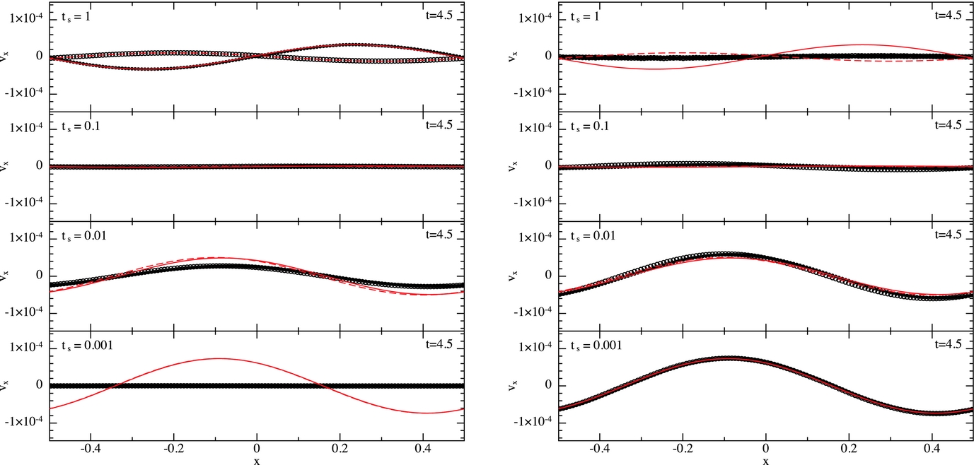
Two-fluid
We perform this test first with the two-fluid algorithm, using 64 × 12 × 12 gas particles and 64 × 12 × 12 dust particles set up on a uniform, close-packed lattice in a periodic box with x ∈ [− 0.5, 0.5] and the y and z boundaries set to correspond to 12 particle spacings on the chosen lattice. The wave is set to propagate along the x-axis with v g = v d = Asin(2πx), ρ = ρ0[1 + Asin(2πx)] with ρ0 = 1 and A = 10−4. The density perturbation is initialised using stretch mapping (Section 3.2; see also Appendix B in Price & Monaghan Reference Price and Monaghan2004b). We perform this test using an adiabatic EOS with c s, 0 = 1. We adopt a simple, constant K drag prescription, choosing K = 0.5, 5, 50, and 500 such that the stopping time given by (236) is a multiple of the wave period (t s = 1, 0.1, 0.01, and 0.001, respectively).
The left panels in Figure 47 show the results of this test using the two-fluid method, showing velocity in each phase compared to the analytic solution after 4.5 wave periods (the time is chosen to give a phase offset between the phases). For stopping times t s ≳ 0.1, the numerical solution matches the analytic solution to within 4%. For short stopping times, Laibe & Price (Reference Laibe and Price2012a) showed that the resolution criterion h ≲ c st s needs to be satisfied to avoid overdamping of the mixture. For the chosen number of particles, the smoothing length is h = 0.016, implying in this case that the criterion is violated when t s ≲ 0.016. This is evident from the lower two panels in Figure 47, where the numerical solution is overdamped compared to the analytic solution.
This problem is not unique to SPH codes, but represents a fundamental limitation of two-fluid algorithms in the limit of short stopping times due to the need to resolve the physical separation between the phases (which becomes ever smaller as t s decreases) when they are modelled with separate sets of particles (or with a grid and a physically separate set of dust particles). The need to resolve a physical length scale results in first-order convergence of the algorithm in the limit of short stopping times, as already noticed by Miniati (Reference Miniati2010) in the context of grid-based codes. The problem is less severe when the dust fraction is small (Lorén-Aguilar & Bate Reference Lorén-Aguilar and Bate2014), but is difficult to ameliorate fully.
One-fluid
The limit of short stopping time (small grains) is the limit in which the mixture is well described by the one-fluid formulation in the terminal velocity approximation (Section 2.13.12). To compare and contrast the two methods for simulating dust in Phantom, the right half of Figure 47 shows the results of the dustywave test computed with the one-fluid method. To perform this test, we set up a single set of 64 × 12 × 12 ‘mixture’ particles placed on a uniform closepacked lattice, with an initially uniform dust fraction ε = 0.5. The particles are given a mass corresponding to the combined mass of the gas and dust, with the density perturbation set as previously.
The one-fluid solution is accurate precisely where the two-fluid method is inaccurate, and vice-versa. For short stopping times (t s = 0.001; bottom row) the numerical solution is within 1.5% of the analytic solution, compared to errors greater than 60% for the two-fluid method (left figure). For long stopping times (t s ≲ 1; top two rows), the one-fluid method is both inaccurate and slow, but this is precisely the regime in which the two-fluid method (left figure) is explicit and therefore cheap. Thus, the two methods are complementary.
5.9.3. Dust diffusion
A simple test of the one-fluid dust diffusion algorithm is given by PL15. For this test, we set up the particles on a uniform cubic lattice in a 3D periodic box x, y, z ∈ [− 0.5, 0.5] using 32 × 32 × 32 particles with an initial dust fraction set according to
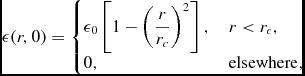 $$\begin{equation}
\epsilon (r,0) = \left\lbrace \arraycolsep5pt\begin{array}{@{}ll@{}}\epsilon _{0} \left[ 1 - \left( \displaystyle\frac{r}{r_{c}} \right)^{2} \right], & r < r_{c}, \\[6pt]
0, & \textrm {elsewhere}, \end{array}\right.
\end{equation}$$
$$\begin{equation}
\epsilon (r,0) = \left\lbrace \arraycolsep5pt\begin{array}{@{}ll@{}}\epsilon _{0} \left[ 1 - \left( \displaystyle\frac{r}{r_{c}} \right)^{2} \right], & r < r_{c}, \\[6pt]
0, & \textrm {elsewhere}, \end{array}\right.
\end{equation}$$
with ε0 = 0.1 and r c = 0.25. We then evolve the dust diffusion equation, (272), discretised according to (279), while setting the acceleration and thermal energy evolution to zero and assuming P = ρ, with the stopping time set to a constant t s = 0.1 and the computational timestep set to Δt = 0.05. Figure 48 shows the evolution of the dust fraction ε ≡ ρd/ρ as a function of radius at various times, showing the projection of all particles in the box (points) compared to the exact solution (red lines) at t = 0.0, 0.1, 0.3, 1.0, and 10.0 (top to bottom). The solution shows a close match to the analytic solution, with agreement to within 0.3% of the analytic solution at all times.
Dust diffusion test from Price & Laibe (Reference Price and Laibe2015a), showing the evolution of the dust fraction on the particles (black dots) as a function of radius at six different times (top to bottom), which may be compared to the analytic solution given by the red lines.
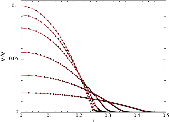
5.9.4. Dust settling
We perform the dust settling test from PL15 in order to directly compare the Phantom solutions to those produced in PL15 with the ndspmhd code. To simplify matters, we do not consider rotation but simply adapt the 2D problem to 3D by using a thin Cartesian box (as for several of the MHD tests in Section 5.6). Our setup follows PL15, considering a slice of a protoplanetary disc at R 0 = 50 au in the r–z plane (corresponding to our x and y Cartesian coordinates, respectively) with density in the ‘vertical’ direction (y) given by
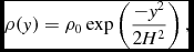 $$\begin{equation}
\rho (y) = \rho _{0} \exp \left( \frac{-y^{2}}{2H^{2}} \right),
\end{equation}$$
$$\begin{equation}
\rho (y) = \rho _{0} \exp \left( \frac{-y^{2}}{2H^{2}} \right),
\end{equation}$$
where we choose H/R 0 = 0.05 giving H = 2.5 au. We use an isothermal EOS with sound speed c s ≡ HΩ, where 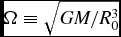 $\Omega \equiv \sqrt{GM/R_{0}^{3}}$, corresponding to an orbital time t orb ≡ 2π/Ω ≈ 353 yr. We adopt code units with a distance unit of 10 au, mass in solar masses, and time units such that G = 1, giving an orbital time of ≈70.2 in code units. We apply an external acceleration in the form
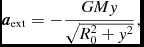 $$\begin{equation}
{\bm a}_{\rm ext} = -\frac{GM y}{\sqrt{{R_{0}^{2} + y^{2}}}},
\end{equation}$$
$$\begin{equation}
{\bm a}_{\rm ext} = -\frac{GM y}{\sqrt{{R_{0}^{2} + y^{2}}}},
\end{equation}$$
where G = M = 1 in code units.
The particles are placed initially on a close-packed lattice using 32 × 110 × 24 = 84480 particles in the domain  $[x,y,z] \in [\pm 0.25,\pm 3H, \pm \sqrt{3/128}]$. We then use the stretch mapping routine (Section 3.2) to give the density profile according to (330). We set the mid-plane density to 10−3 in code units, or ≈6 × 10⁻¹³g cm−3. The corresponding particle mass in code units is 1.13 × 10⁻⁹. We use periodic boundaries, with the boundary in the y direction set at ±10H to avoid periodicity in the vertical direction.
Following the procedure in PL15, we relax the density profile by evolving for 15 orbits with gas only with damping switched on. We then restart the calculation with either (i) a dust fraction added to each particle (one-fluid) or (ii) a corresponding set of dust particles duplicated from the gas particles (two-fluid). For the dust, we assume 1-mm grains with an Epstein drag prescription, such that the stopping time is given by (250). Since Δv is not available when computing t s with the one-fluid method, we set the factor f = 1 in (250) when using this method (this is a valid approximation since by definition Δv is small when the one-fluid method is applicable). The dimensionless stopping time t sΩ = 8.46 × 10⁻³ initially at the disc midplane. After adding dust, we continued the simulation for a further 50 orbits.
Figure 49 shows the dust density at intervals of 10 t orb, showing the cross-section slice through the z = 0 plane of the 3D box which may be directly compared to the 2D solutions shown in PL15. Settling of the dust layer proceeds as expected, with close agreement between the one-fluid (top row) and two-fluid (bottom row) methods, though the two-fluid method is much slower for this test because of the timestep constraint imposed by the stopping time, c.f. (261). The dust resolution is higher in the two-fluid calculation because the set of dust particles follow the dust mass rather than the total mass (for the one-fluid method).
3D version of the dust settling test from Price & Laibe (Reference Price and Laibe2015a), showing the dust density in the ‘r–z’ plane of a protoplanetary disc. We assume mm-sized grains with a 1% initial dust-to-gas ratio in a stratified disc atmosphere with H/R 0 = 0.05 with R 0 = 50 au in (331).
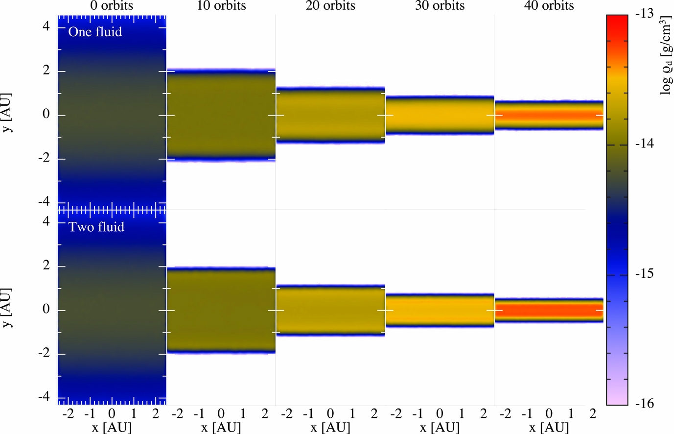
5.10. ISM cooling and chemistry
Figure 50 shows the behaviour of the various cooling and chemistry modules used when modelling the ISM. These plots were made from the data from a simulation of gas rings embedded in a static background potential giving a flat rotation curve (Binney & Tremaine Reference Binney and Tremaine1987). Gas is setup in a ring of constant surface density from 5 to 10 kpc in radius, initially at 10 000 K, with a total gas mass of 2 × 10⁹ M⊙. The top panels show a temperature and pressure profile of all gas particles. The temperature plateaus around 10 000 K and forms a two-phase medium visible in the ‘knee’ in the pressure profile, as expected for ISM thermal models (Wolfire et al. Reference Wolfire, Hollenbach, McKee, Tielens and Bakes1995). Much lower temperatures can be reached if the gas is given a higher surface density or if self-gravity is active. In the case of the latter, some energy delivery scheme, or the inclusion of a large number of sink particles, is needed to break apart the cold knots.
Temperature and pressure profiles resulting from the ISM heating and cooling functions (top) and the abundances of H2 and CO as a function of gas density (bottom). The behaviour of the H2 and CO fractions close to n = 10cm−3 is a consequence of H2 self-shielding: In gas which was initially molecular, this remains effective down to lower densities than is the case in gas which was initially atomic. This behaviour is discussed in much greater detail in Dobbs et al. (Reference Dobbs, Glover, Clark and Klessen2008).
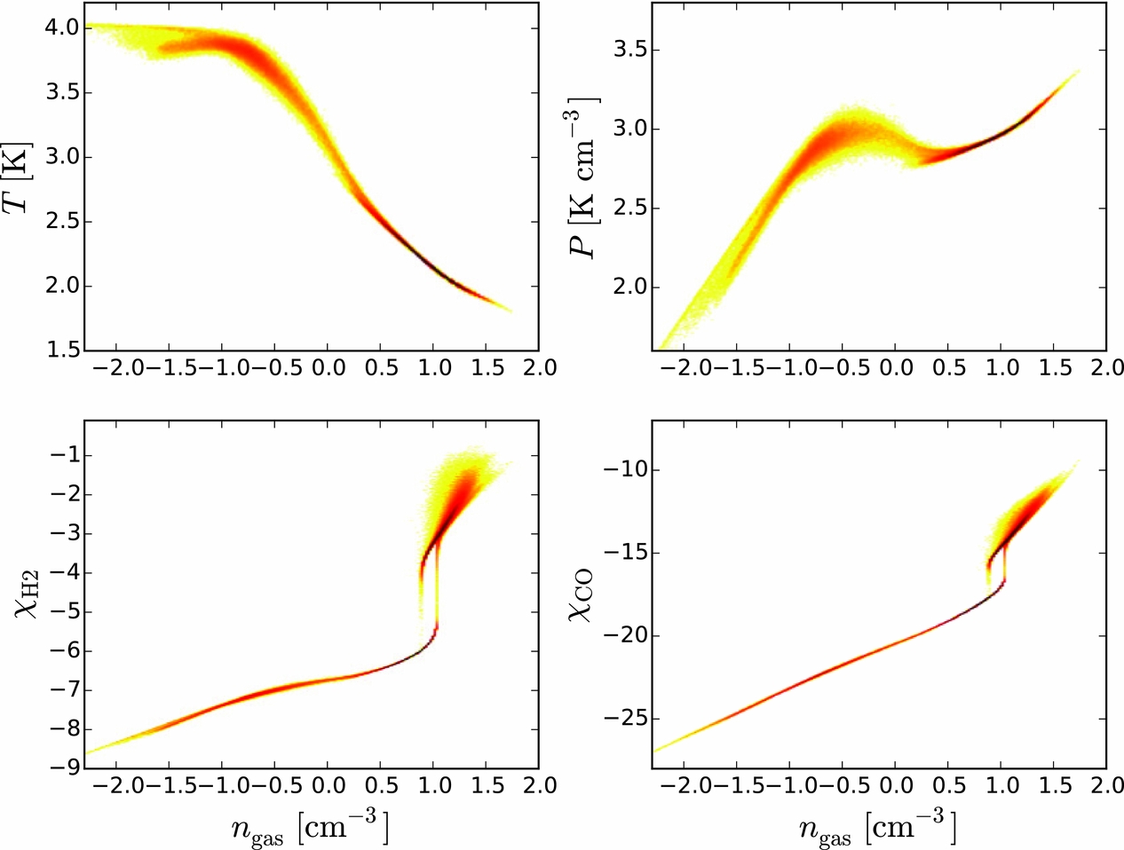
The bottom two panels of Figure 50 show the chemical abundances of H2 and CO. The exact form of the molecular abundance profiles are a function of many variables that are set at run time, with the data in the figure made from the default values. The molecular abundances are strong functions of total gas density, with the CO being a strong function of H2 abundance. If a higher gas mass (e.g. × 10 the value used here) or self-gravity is included then abundances reach a maximum of either 0.5 for H2 or the primordial carbon abundance for CO. See Dobbs et al. (Reference Dobbs, Glover, Clark and Klessen2008) for a detailed discussion of the features of these abundance curves.
6 EXAMPLE APPLICATIONS
Phantom is already a mature code, in the sense that we have always developed the code with specific applications in mind. In this final section, we demonstrate five example applications for which the code is well suited. The setup for each of these applications are provided in the wiki documentation so they can be easily reproduced by the novice user. We also plan to incorporate these examples into an ‘optimisation suite’ to benchmark performance improvements to the code.
6.1. Supersonic turbulence
Our first example application employs the turbulence forcing module described in Section 2.5. Figure 51 shows the gas column density in simulations of isothermal supersonic turbulence driven to an rms Mach number of  $\mathcal {M} \approx 10$, identical to those performed by Price & Federrath (Reference Price and Federrath2010). The calculations use 2563 particles and were evolved for 10 turbulent crossing times, $t_{\rm c} = L / (2 \mathcal {M})$. This yields a crossing time of t c = 0.05 in code units. The gas is isothermal with sound speed c s = 1 in code units. The initial density is uniform ρ0 = 1.
Gas column density in Phantom simulations of driven, isothermal, supersonic turbulence at Mach 10, similar to the calculations performed by Price & Federrath (Reference Price and Federrath2010). We show the numerical solutions at t = 1, 2, and 3 crossing times (left to right, respectively). The colour scale is logarithmic between 10−1 and 10 in code units.
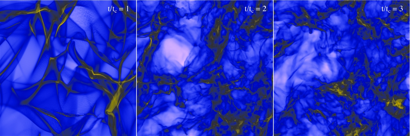
The gas column density plots in Figure 51 may be directly compared to the panels in Figure 3 of Price & Federrath (Reference Price and Federrath2010). Figure 52 shows the time-averaged probability distribution function (PDF) of s ≡ ln(ρ/ρ0). This demonstrates the characteristic signature of isothermal supersonic turbulence, namely the appearance of a log-normal PDF in s (e.g. Vazquez-Semadeni Reference Vazquez-Semadeni1994; Nordlund & Padoan Reference Nordlund, Padoan, Franco and Carraminana1999; Ostriker, Gammie, & Stone Reference Ostriker, Gammie and Stone1999). Indeed, Phantom was used in the study by Price, Federrath, & Brunt (Reference Price, Federrath and Brunt2011) to confirm the relationship between the standard deviation and the Mach number in the form
 $$\begin{equation}
\sigma _{\rm s}^{2} = \ln \left( 1 + b^{2} \mathcal {M}^{2} \right),
\end{equation}$$
$$\begin{equation}
\sigma _{\rm s}^{2} = \ln \left( 1 + b^{2} \mathcal {M}^{2} \right),
\end{equation}$$
where b = 1/3 for solenoidally driven turbulence, as earlier suggested by Federrath et al. (Reference Federrath, Klessen and Schmidt2008, Reference Federrath, Roman-Duval, Klessen, Schmidt and Mac Low2010a).
Time-averaged PDF of s = ln(ρ/ρ0) for supersonic Mach 10 turbulence, with the shaded region representing the standard deviation of the averaging. The PDF is close to a log-normal distribution, shown by the dashed red line.
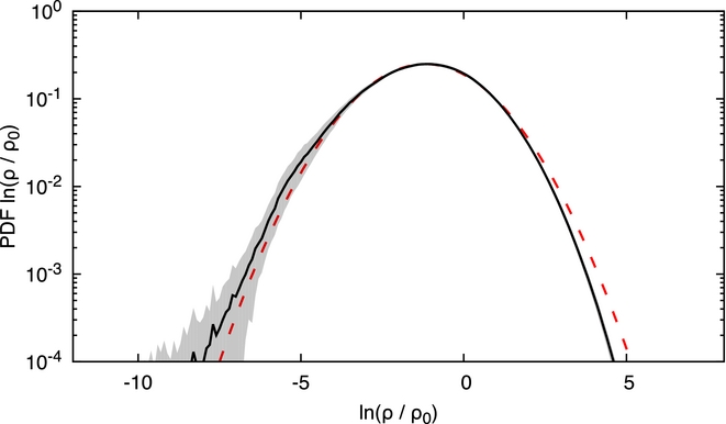
6.2. Star cluster formation
SPH has been used to study star formation since the earliest studies by Gingold & Monaghan (Reference Gingold and Monaghan1982a, Reference Gingold and Monaghan1983), Phillips (Reference Phillips1982, Reference Phillips1986a, Reference Phillips1986b), and Monaghan & Lattanzio (Reference Monaghan and Lattanzio1986, Reference Monaghan and Lattanzio1991), even motivating the original development of MHD in SPH by Phillips & Monaghan (Reference Phillips and Monaghan1985). The study by Bate et al. (Reference Bate, Bonnell and Bromm2003) represented the first simulation of ‘large-scale’ star cluster formation, resolved to the opacity limit for fragmentation (Rees Reference Rees1976; Low & Lynden-Bell Reference Low and Lynden-Bell1976). This was enabled by the earlier development of sink particles by Bate et al. (Reference Bate, Bonnell and Price1995), allowing star formation simulations to continue beyond the initial collapse (Bonnell et al. Reference Bonnell, Bate, Clarke and Pringle1997; Bate & Bonnell Reference Bate and Bonnell1997). This heritage is present in Phantom which inherits many of the ideas and algorithms implemented in the sphng code.
Figure 53 shows a series of snapshots taken from a recent application of Phantom to star cluster formation by Liptai et al. (Reference Liptai, Price, Wurster and Bate2017). The initial setup follows Bate et al. (Reference Bate, Bonnell and Bromm2003)—a uniform density sphere of 0.375 pc in diameter with a mass of 50 M⊙. The initial velocity field is purely solenoidal, generated on a 643 uniform grid in Fourier space to give a power spectrum P(k)∝k −4 consistent with the Larson (Reference Larson1981) scaling relations, and then linearly interpolated from the grid to the particles. The initial kinetic energy is set to match the gravitational potential energy, (3/5GM 2/R), giving a root mean square Mach number ≈6.4. We set up 3.5 × 10⁶ particles in the initial sphere placed in a uniform random distribution. We evolve the simulation using a barotropic EOS P = Kργ in the form
 $$\begin{equation}
\frac{P}{\rho } = \left\lbrace \arraycolsep5pt\begin{array}{@{}ll@{}}c^2_{{\rm s}, 0}, & \rho < \rho _1, \\[3pt]
c^2_{{\rm s}, 0} \left( \displaystyle\frac{\rho }{\rho _1}\right)^{(\gamma _1 - 1)}, & \rho _1 \le \rho < \rho _2, \\[3pt]
c^2_{{\rm s}, 0} \left( \displaystyle\frac{\rho _2}{\rho _1}\right)^{(\gamma _1 - 1)} \left( \displaystyle\frac{\rho }{\rho _1}\right)^{(\gamma _2 - 1)}, & \rho _2 \le \rho < \rho _3, \\[3pt]
c^2_{{\rm s}, 0} \left( \displaystyle\frac{\rho _2}{\rho _1}\right)^{(\gamma _1 - 1)} \left( \displaystyle\frac{\rho _3}{\rho _2}\right)^{(\gamma _2 - 1)} \left( \displaystyle\frac{\rho }{\rho _3} \right)^{(\gamma _3 - 1)}, & \rho \ge \rho _3, \end{array}\right.
\end{equation}$$
$$\begin{equation}
\frac{P}{\rho } = \left\lbrace \arraycolsep5pt\begin{array}{@{}ll@{}}c^2_{{\rm s}, 0}, & \rho < \rho _1, \\[3pt]
c^2_{{\rm s}, 0} \left( \displaystyle\frac{\rho }{\rho _1}\right)^{(\gamma _1 - 1)}, & \rho _1 \le \rho < \rho _2, \\[3pt]
c^2_{{\rm s}, 0} \left( \displaystyle\frac{\rho _2}{\rho _1}\right)^{(\gamma _1 - 1)} \left( \displaystyle\frac{\rho }{\rho _1}\right)^{(\gamma _2 - 1)}, & \rho _2 \le \rho < \rho _3, \\[3pt]
c^2_{{\rm s}, 0} \left( \displaystyle\frac{\rho _2}{\rho _1}\right)^{(\gamma _1 - 1)} \left( \displaystyle\frac{\rho _3}{\rho _2}\right)^{(\gamma _2 - 1)} \left( \displaystyle\frac{\rho }{\rho _3} \right)^{(\gamma _3 - 1)}, & \rho \ge \rho _3, \end{array}\right.
\end{equation}$$
where we set the initial sound speed c s, 0 = 2 × 104 cm s−1 and set [ρ1, ρ2, ρ3] = [10−13, 10−10, 10−3] g cm−3 and [γ1, γ2, γ3] = [1.4, 1.1, 5/3], as in Bate et al. (Reference Bate, Bonnell and Bromm2003). We turn on automatic sink particle creation with a threshold density of 10−10 g cm−3, with sink particle accretion radii set to 5 au and particles accreted without checks at 4 au. No sink particles are allowed to be created within 10 au of another existing sink. The calculations satisfy the Bate & Burkert (Reference Bate and Burkert1997) criterion of resolving the minimum Jeans mass in the calculation (known as the opacity limit for fragmentation; Rees Reference Rees1976; Low & Lynden-Bell Reference Low and Lynden-Bell1976) by at least the number of particles contained within one smoothing sphere.
Star cluster formation with Phantom, showing snapshots of gas column density during the gravitational collapse of a 50 M⊙ molecular cloud core, following Bate, Bonnell, & Bromm (Reference Bate, Bonnell and Bromm2003). Snapshots are shown every 0.2 tff (left to right, top to bottom), with the panels after t > t ff zoomed in to show the details of the star formation sequence. As in Bate et al. (Reference Bate, Bonnell and Bromm2003), we resolve the fragmentation to the opacity limit using a barotropic equation of state.
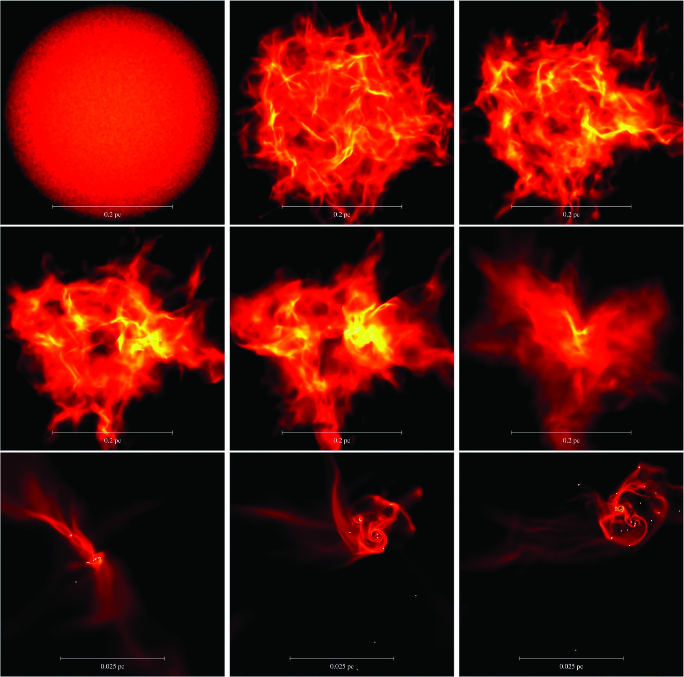
The snapshots shown in Figure 53 show a similar evolution to the original calculation of Bate et al. (Reference Bate, Bonnell and Bromm2003). The evolution is not identical since we used a different realisation of the initial turbulent velocity field. A more quantitative comparison can be found in Liptai et al. (Reference Liptai, Price, Wurster and Bate2017) where we performed seven different realisations of the collapse in order to measure a statistically meaningful initial mass function (IMF) from the calculations, finding an IMF in agreement with the one found by Bate (Reference Bate2009a) in a much larger (500 M⊙) calculation. The IMF produced with a barotropic EOS does not match the observed local IMF in the Milky Way (e.g. Chabrier Reference Chabrier, Corbelli, Palle and Zinnecker2005), tending to over-produce low mass stars and brown dwarfs. This is a known artefact of the barotropic EOS (e.g. Matzner & Levin Reference Matzner and Levin2005; Krumholz Reference Krumholz2006; Bate Reference Bate2009b), since material around the stars remains cold rather than being heated. It can be fixed by implementing radiative feedback, for example, by implementing radiation hydrodynamics in the flux-limited diffusion approximation (Whitehouse & Bate Reference Whitehouse and Bate2004; Whitehouse, Bate, & Monaghan Reference Whitehouse, Bate and Monaghan2005; Whitehouse & Bate Reference Whitehouse and Bate2006). This is not yet implemented in Phantom but it is high on the agenda.
6.3. Magnetic outflows during star formation
Phantom may also be used to model the formation of individual protostars. We present an example following the initial setup and evolution of Price et al. (Reference Price, Tricco and Bate2012). A molecular cloud core with initial density ρ0 = 7.4 × 10⁻¹⁸ g cm−3 is embedded in pressure equilibrium with ambient medium of density 2.5 × 10⁻¹⁹ g cm−3. The barotropic EOS given by (333) is used, setting c s = 2.2 × 104 cm s−1. The radius of the core is 4 × 1016 cm (≈2700 au), with the length of the cubic domain spanning [x, y, z] = ±8 × 1016 cm. The core is in solid body rotation with angular speed Ω = 1.77 × 10⁻¹³ rad s−1. The magnetic field is uniform and aligned with the rotation axis with a mass-to-flux ratio μ = 5, corresponding to B 0 ≈ 163 μG. A sink particle is inserted once the gas reaches a density of 10−10 g cm−3, with an accretion radius of 5 au. Thus, this calculation models only the evolution of the first hydrostatic core phase of star formation. The core is composed of 1004255 particles, with 480033 particles in the surrounding medium.
Figure 54 shows the evolution of a magnetised, collimated bipolar jet of material, similar to that given by Price et al. (Reference Price, Tricco and Bate2012). Infalling material is ejected due to the wind up of the toroidal magnetic field. The sink particle is inserted at t ≈ 25 400 yrs, shortly before the jet begins. The jet continues to be driven, while material continues to infall, lasting for several thousand years.
Magnetically propelled jet of material bursting out of the first hydrostatic core phase of star formation.
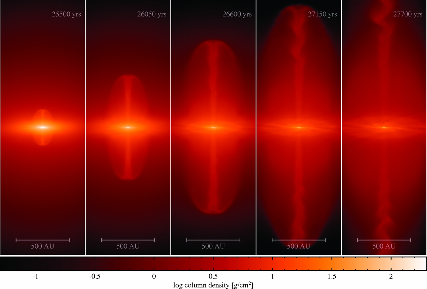
6.4. Galaxy merger
To provide a realistic test of the collisionless N-body and SPH implementations, we performed a comparison study where we modelled a galaxy merger, comparing the Phantom results with the Hydra N-body/SPH code (Couchman, Thomas, & Pearce Reference Couchman, Thomas and Pearce1995; Thacker & Couchman Reference Thacker and Couchman2006). This test requires gravity along with multiple particle types—gas, stars, and dark matter. Gas interacts hydrodynamically only with itself, and all three particle types interact with each other via gravity (c.f. Table A1).
To create a Milky Way-like galaxy, we used GalactICs (Kuijken & Dubinski Reference Kuijken and Dubinski1995b; Widrow & Dubinski Reference Widrow and Dubinski2005; Widrow, Pym, & Dubinski Reference Widrow, Pym and Dubinski2008) to first create a galaxy consisting of a stellar bulge, stellar disc, and a dark matter halo. To create the gas disc, the stellar disc was then duplicated and reflected in the x = y plane to avoid coincidence with the star particles. Ten percent of the total stellar mass was then removed and given to the gas disc. Although the gas disc initially has a scale height larger than physically motivated, this will quickly relax into a disc that physically resembles the Milky Way. Next, we added a hot gas halo embedded within the dark matter halo. The hot gas halo has an observationally motivated β-profile (e.g. Cavaliere & Fusco-Femiano Reference Cavaliere and Fusco-Femiano1976) and a temperature profile given by Kaufmann et al. (Reference Kaufmann, Mayer, Wadsley, Stadel and Moore2007); the mass of the hot gas halo is removed from the dark matter particles to conserve total halo mass. The mass of each component, as well as particle numbers and particle masses are given in Table 5. To model the major merger, the galaxy is duplicated and the two galaxies are placed 70 kpc apart on a parabolic trajectory. These initial conditions are identical to those used in Wurster & Thacker (Reference Wurster and Thacker2013b, Reference Wurster and Thacker2013a). To simplify the comparison, there is no star formation recipe, no black holes, and no feedback from active galactic nuclei (there are currently no plans to implement cosmological recipes in Phantom). Thus, only the SPH and gravity algorithms are being compared.
Component breakdown for each galaxy. For each component, the total mass is M, the particle mass is m, and the number of particles is N.
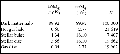
Figure 55 shows the gas column density evolution from t = 100 Myr to t = 1.4 Gyr, comparing Phantom (left) to Hydra (right), and Figure 56 shows the evolution of the separation of the galaxies and the mean and maximum gas density in each model. The evolution of the two galaxy mergers agree qualitatively with one another, with slight differences in the trajectories, evolution times, and gas densities between the two codes. Using the centre of mass of the star particles that were assigned to each galaxy as a proxy for the galaxy’s centre, the maximum separation at t ≈ 450 Myr is 59 and 61 kpc for Hydra and Phantom, respectively. Second, periapsis occurs at 875 and 905 Myr for Hydra and Phantom, respectively, which is a difference of 3.4% since the beginning of the simulation. The maximum gas density is approximately two times higher in Phantom prior to the merger, and about 1.2 times higher after the merger; the average gas densities typically differ by less than a factor of 1.2 both before and after the merger.
Evolution of the gas column density in a major merger of two Milky Way-sized galaxies, comparing Phantom to the Hydra code. Times shown are from the onset of the simulation, with each frame (100 kpc)2. The colour bar is log [column density/(M⊙ pc−1)].
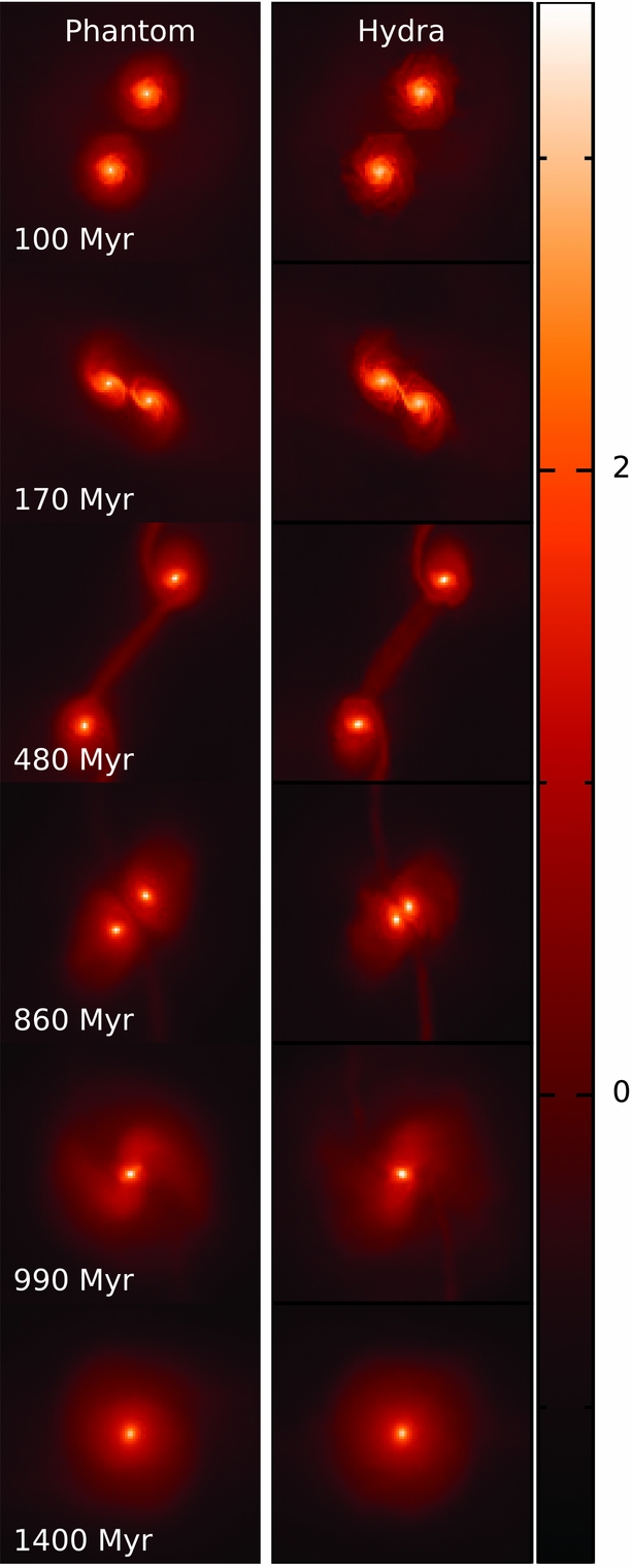
Top: The evolution of the separation of the galaxies, using centre of mass of the star particles that were assigned to each galaxy as a proxy for the galaxy’s centre; the stars are sufficiently mixed after 1000 Myr, thus a meaningful separation cannot be calculated. Bottom: The evolution of the maximum (solid) and mean (dashed) gas densities for each model.
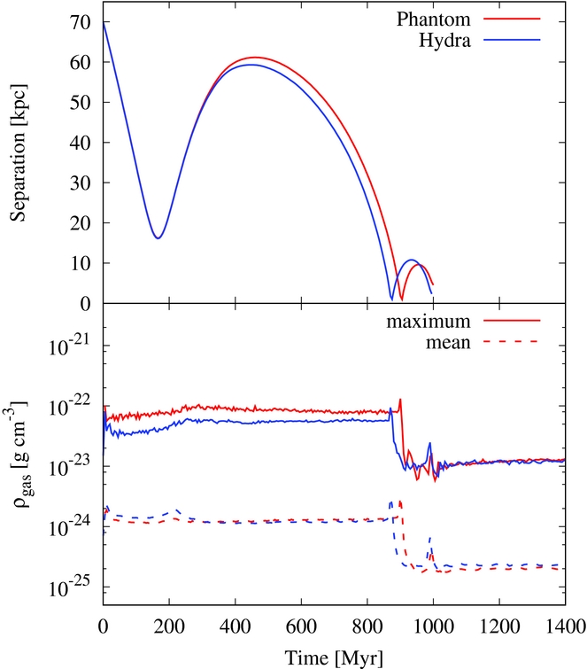
There are several differences in the algorithms used in Hydra compared to Phantom. The first is the gravity solver. The long-range gravity in Hydra uses an adaptive particle-mesh algorithm (Couchman Reference Couchman1991), while Phantom uses a kd-tree (c.f. Section 2.12.4). For the short-range gravity, Hydra uses a fixed S2 softening length for all particles, where the S2 softening is scaled to an equivalent Plummer softening such that εS2 = 2.34εPlummer; for this simulation, εi ≡ εPlummer = 300 pc. In Phantom, εi = h i for each particle, where h i is calculated using only the particles of the same type as particle i.
A second difference is the treatment of the smoothing length in high density regions. In Hydra, as is common in most galactic and cosmological codes, the smoothing length is limited such that h i = max(h i, h min), where h min = εPlummer/8( = 37.5 pc). In Phantom, h i is always calculated self-consistently and thus has no imposed lower limit.
Finally, Phantom contains an artificial conductivity term (Section 2.2.8) that acts to ensure continuous pressure fields across contact discontinuities (Price Reference Price2008).
In Wurster & Thacker (Reference Wurster and Thacker2013b), the Hydra major merger model was compared to a simulation run using the publicly available version of Gadget2 (Springel et al. Reference Springel, Yoshida and White2001; Springel & Hernquist Reference Springel and Hernquist2002). As here, the comparison was simplified such that only the gravity and SPH solvers were being compared. They found that the galaxies in each simulation followed similar trajectories and both models reached second periapsis within 0.2% of one another, as measured from the beginning of the simulation. Note that both Hydra and Gadget2 were both written primarily to solve galactic and cosmological models.
The quantitive difference in results may be attributed to the improved SPH algorithms in Phantom compared to Hydra. The higher density in Hydra is consistent with the results in Richardson et al. (Reference Richardson, Scannapieco, Devriendt, Slyz, Thacker, Dubois, Wurster and Silk2016), who found higher densities in Hydra compared to the adaptive mesh refinement code Ramses (Teyssier Reference Teyssier2002). It was determined that this was a result of a combination of the artificial viscosity, h min and the suppression of ‘mixing’ (which occurs when no thermal conductivity is applied).
6.5. Gap opening in dusty discs
Our final example is taken from Dipierro et al. (Reference Dipierro, Laibe, Price and Lodato2016) and builds on our recent studies of dust dynamics in protoplanetary discs with Phantom (e.g. Dipierro et al. Reference Dipierro, Price, Laibe, Hirsh and Cerioli2015; Ragusa et al. Reference Ragusa, Dipierro, Lodato, Laibe and Price2017). We perform calculations using the two-fluid approach, setting up a disc with 500 000 gas particles and 100 000 dust particles with Σ∝r −0.1 between 1 and 120 au with a total disc mass of 2 × 10⁻⁴ M⊙. The disc mass is chosen to place the mm dust particles in a regime where the Stokes number is greater than unity. The initial dust-to-gas ratio is 0.01 and we assume a locally isothermal EOS with c s∝r −0.35, normalised such that H/R = 0.05 at 1 au. We use the minimum disc viscosity possible, setting αAV = 0.1.
Figure 57 shows the results of two calculations employing planets of mass 0.1 M Jupiter (top row) and 1.0 M Jupiter (bottom) embedded in a disc around a 1.3 M⊙ star. Left and right panels show gas and dust surface densities, respectively. While the theory of gap opening in gaseous discs is relatively well understood as a competition between the gravitational torque from the planet trying to open a gap and the viscous torques trying to close it (e.g. Goldreich & Tremaine Reference Goldreich and Tremaine1979, Reference Goldreich and Tremaine1980), gap opening in dusty discs is less well understood (see e.g. Paardekooper & Mellema Reference Paardekooper and Mellema2004, Reference Paardekooper and Mellema2006). In Dipierro et al. (Reference Dipierro, Laibe, Price and Lodato2016), we identified two regimes for gap opening in dusty discs where gap opening in the dust disc is either resisted or assisted by the gas–dust drag. The top row of Figure 57 demonstrates that low mass planets can carve a gap which is visible only in the dust disc, while for high mass planets (bottom row), there is a gap opened in both gas and dust but it is deeper in the dust. Moreover, the gap opening mechanism by low mass planets has been further investigated in Dipierro & Laibe (Reference Dipierro and Laibe2017). They derived a grain size-dependent criterion for dust gap opening in discs, an estimate of the location of the outer edge of the dust gap and an estimate of the minimum Stokes number above which low-mass planets are able to carve gaps which appear only in the dust disc. These predictions has been tested against Phantom simulations of planet–disc interaction in a broad range of dusty protoplanetary discs, finding a remarkable agreement between the theoretical model and the numerical experiments.
Gap opening in dusty protoplanetary discs with Phantom (from Dipierro et al. Reference Dipierro, Laibe, Price and Lodato2016), showing surface density in gas (left) and mm dust grains (right) in two simulations of planet–disc interaction with planet masses of 0.1 MJupiter (top) and 1 MJupiter (bottom) in orbit around a 1.3 M⊙ star. In the top case, a gap is opened only in the dust disc, while in the bottom row, the gap is opened in both gas and dust. The colour bar is logarithmic surface density in cgs units.
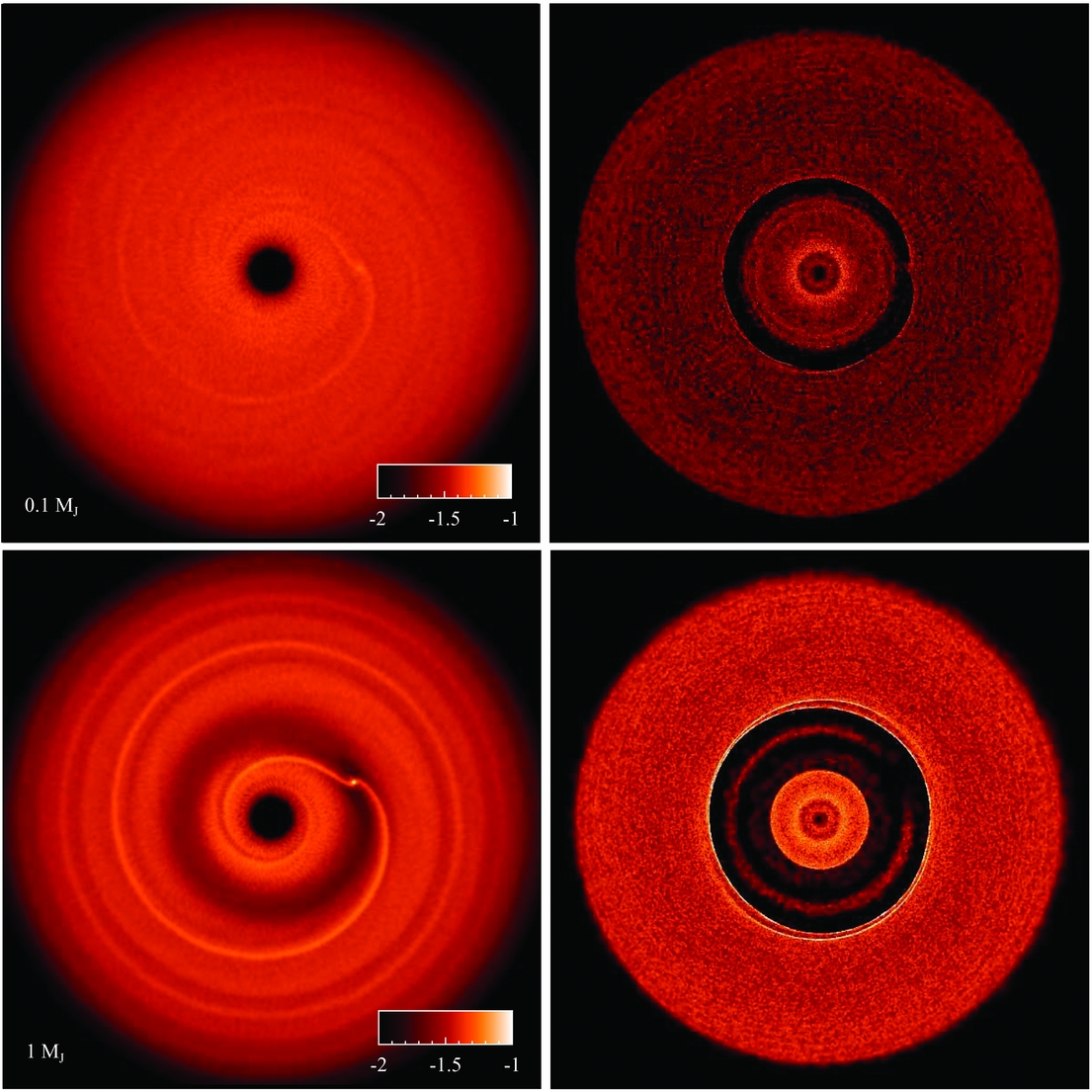
Interestingly, our prediction of dust gaps that are not coincident with gas gaps for low mass planets appears to be observed in recent observations of the TW Hya protoplanetary disc, by comparing VLT-SPHERE imaging of the scattered light emission from small dust grains (van Boekel et al. Reference van Boekel2017; tracing the gas) to ALMA images of the mm dust emission (Andrews et al. Reference Andrews2016).
7 SUMMARY
We have outlined the algorithms and physics currently implemented in the Phantom SPH and MHD code in the hope that this will prove useful to both users and developers of the code. We have also demonstrated the performance of the code as it currently stands on a series of standard test problems, most with known or analytic solutions. While no code is ever ‘finished’ nor bug free, it is our hope that the code as it stands will prove useful to the scientific community. Works in progress for future code releases include radiation hydrodynamics, continuing development of the dust algorithms, and an implementation of relativistic hydrodynamics.
ACKNOWLEDGEMENTS
Phantom is the result of interactions over the years with numerous talented and interesting people. Particular mentions go to Joe Monaghan, Matthew Bate, and Stephan Rosswog from whom I (DP) learnt and discussed a great deal about SPH over the years. We also thank Walter Dehnen, James Wadsley, Evghenii Gaburov, Matthieu Viallet, and Pedro Gonnet for stimulating interactions. This work and the public release of Phantom was made possible by the award of a four-year Future Fellowship (FT130100034) to DJP from the Australian Research Council (ARC), as well as funding via Discovery Projects DP130102078 (funding James Wurster and Mark Hutchison) and DP1094585 (which funded Guillaume Laibe and partially funded Terrence Tricco). CN is supported by the Science and Technology Facilities Council (grant number ST/M005917/1). CF gratefully acknowledges funding provided by ARC Discovery Projects (grants DP150104329 and DP170100603). SCOG acknowledges support from the Deutsche Forschungsgemeinschaft via SFB 881 (sub-projects B1, B2, B8) and from the European Research Council via the ERC Advanced Grant ‘STARLIGHT’ (project number 339177). This work was supported by resources awarded under Astronomy Australia Ltd’s merit allocation scheme on the gSTAR and swinSTAR national facilities at Swinburne University of Technology and the Pawsey National Supercomputing Centre. gSTAR and swinSTAR are funded by Swinburne and the Australian Government’s Education Investment Fund. We thank Charlene Yang from the Pawsey Supercomputing Centre for particular help and assistance as part of a Pawsey uptake project. We used splash for many of the figures (Price Reference Price2007). We thank Max Tegmark for his excellent icosahedron module used in various analysis routines. We thank the three referees of this paper for extensive comments on the manuscript.
A DETAILS OF CODE IMPLEMENTATION
Figure A1 shows the basic structure of the code. The core of the code is the timestepping loop, while the most time consuming part are the repeated calls to evaluate density and acceleration on the particles via sums over neighbouring particles. Further details of these steps are given in Section A.3.
Flowchart showing the basic structure of Phantom. To the user what appears is a sequence of output files written at discrete time intervals. The core of the code is the timestepping loop, while most of the computational cost is spent building the tree and evaluating density and acceleration by summing over neighbours.

A.1 Smoothing kernels
A Python script distributed with Phantom can be used to generate the code module for alternative smoothing kernels, including symbolic manipulation of piecewise functions using sympy to obtain the relevant functions needed for gravitational force softening (see below). Pre-output modules for the six kernels described in Section 2.1.6 are included in the source code, and the code can be recompiled with any of these replacing the default cubic spline on the command line, e.g. make KERNEL=quintic.
The double hump kernel functions used in the two-fluid dust algorithm (Section 2.13.4) can be generated automatically from the corresponding density kernel by the kernels.py script distributed with Phantom, as described in Section 2.12.2. The pre-generated modules implementing each of the kernels described in Section 2.1.6 hence automatically contain the corresponding double hump kernel function, which is used to compute the drag terms.
A.2 Particle types
Particles can be assigned with a ‘type’ from the list (see Table A1 in the appendix). The main use of this is to be able to apply different sets of forces to certain particle types (see description for each type). Densities and smoothing lengths are self-consistently computed for all of these types except for ‘dead’ particles which are excluded from the tree build and boundary particles whose properties are fixed. However, the kernel interpolations used for these involve only neighbours of the same type. Particle masses in Phantom are fixed to be equal for all particles of the same type, to avoid problems with unequal mass particles (e.g. Monaghan & Price Reference Monaghan and Price2006). We use adaptive gravitational force softening for all particle types, both SPH and N-body (see Section 2.12.3). Sink particles are handled separately to these types, being stored in a separate set of arrays, carry only a fixed softening length which is set to zero by default and compute their mutual gravitational force without approximation (see Section 2.8).
Particle types in Phantom. The density and smoothing length of each type is computed only from neighbours of the same type (c.f. Section 2.13.3). Sink particles are handled separately in a different set of arrays.
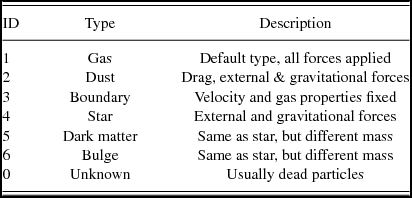
A.3 Evaluating density and acceleration
A.3.1 Tree build
Phantom uses a kd-tree for nearest neighbour finding and to compute long range gravitational accelerations. The procedure for the tree build is given in Figure A2. We use a stack, rather than recursive subroutines, for efficiency and to aid parallelisation (the parallelisation strategy for the tree build is discussed further in Section A.4.2). The stack initially contains only the highest level node for each thread (in serial, this would be the root node). We loop over all nodes on the stack and call a subroutine to compute the node properties, namely the centre of mass position, the node size, s, which is the radius of a sphere containing all the particles centred on the centre of mass, the maximum smoothing length for all the particles contained within the node, pointers to the two node children and the parent node, and, if self-gravity is used, the total mass in the node as well as the quadrupole moment (see Section 2.12). The construct_node subroutine also decides whether or not the node should be split (i.e. if the number of particles >N min) and returns the indices and boundaries of the resultant child nodes.
Pseudo-code for the tree build. The construct_node procedure computes, for a given node, the centre of mass, size, maximum smoothing length, quadrupole moments, and the child and parent pointers and the boundaries of the child nodes.
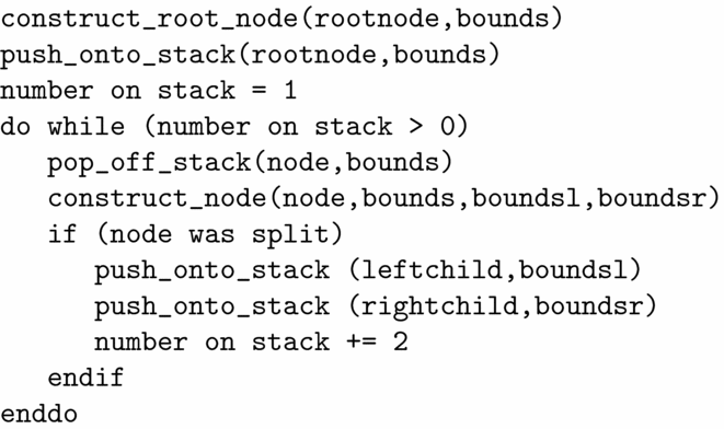
We access the particles by storing an integer array containing the index of the first particle in each node (firstinnode), and using a linked list where each particle stores the index of the next particle in the node (next), with an index of zero indicating the end of the list. During the tree build, we start with only the root node, so firstinnode is simply the first particle that is not dead or accreted and the next array is filled to contain the next non-dead-or-accreted particle using a simple loop. In the construct_node routine, we convert this to a simple list of the particles in each node and use this temporary list to update the linked list when creating the child nodes (i.e., by setting firstinnode to zero for the parent nodes, and filling firstinnode and next for the child nodes based on whether the particle position is to the ‘left’ or the ‘right’ of the bisected parent node).
The tree structure itself stores eight quantities without self-gravity, requiring 52 bytes per particle (x,y,z,size,hmax: 5 × 8-byte double precision; leftchild, rightchild, parent: 3 × 4-byte integer). With self-gravity, we store 15 quantities (mass and quads(6), i.e. seven additional 8-byte doubles) requiring 108 bytes per particle. We implement the node indexing scheme outlined by Gafton & Rosswog (Reference Gafton and Rosswog2011) where the tree nodes on each level l are stored starting from 2l − 1, where level 1 is the ‘root node’ containing all the particles, to avoid the need for thread locking when different sections of the tree are built in parallel. However, the requirement of allocating storage for all leaf nodes on all levels regardless of whether or not they contain particles either limits the maximum extent of the tree or can lead to prohibitive memory requirements, particularly for problems with high dynamic range, such as star formation, where a small fraction of the particles collapse to high density. Hence, we use this indexing scheme only up to a maximum level (maxlevel_indexed) which is set such that 2maxlevel_indexed is less than the maximum number of particles (maxp). We do, however, allow the tree build to proceed beyond this level, whereupon the leftchild, rightchild and parent indices are used and additional nodes are added in the order that they are created (requiring limited thread locking).
A.3.2 Neighbour search
The neighbour search for a given ‘leaf node’, n, proceeds from the top down. As with the tree build, this is implemented using a stack, which initially contains only the root node. The procedure is summarised in Figure A3. We loop over the nodes on the stack, checking the criterion
 $$\begin{equation}
r_{nm}^{2} < (s_{n} + s_{m} + R_{\rm kern} h^{n}_{\rm max})^{2},
\end{equation}$$
$$\begin{equation}
r_{nm}^{2} < (s_{n} + s_{m} + R_{\rm kern} h^{n}_{\rm max})^{2},
\end{equation}$$
where r 2nm ≡ (xn − xm)2 + (yn − ym)2 + (zn − zm)2 is the square of the separation between the node centres and s is the node size. Any node m satisfying this criteria, that is not a leaf node, has its children added to the stack and the search continues. If node m is a leaf node, then the list of particles it contains are added to the trial neighbour list and the positions cached. The end product is a list of trial neighbours (listneigh), its length nneigh, and a cache containing the trial neighbour positions (xyzcache) up to some maximum size (12 000 by default, the exact size not being important except that it is negligible compared to the number of particles). Trial neighbours exceeding this number are retrieved directly from memory during the density calculation rather than from the cache. This occurs rarely, but the overflow mechanism allows for the possibility of a few particles with a large number of neighbours, as happens under certain circumstances.
Pseudo-code for the neighbour search (referred to as the get_neigh routine in Figure A4).
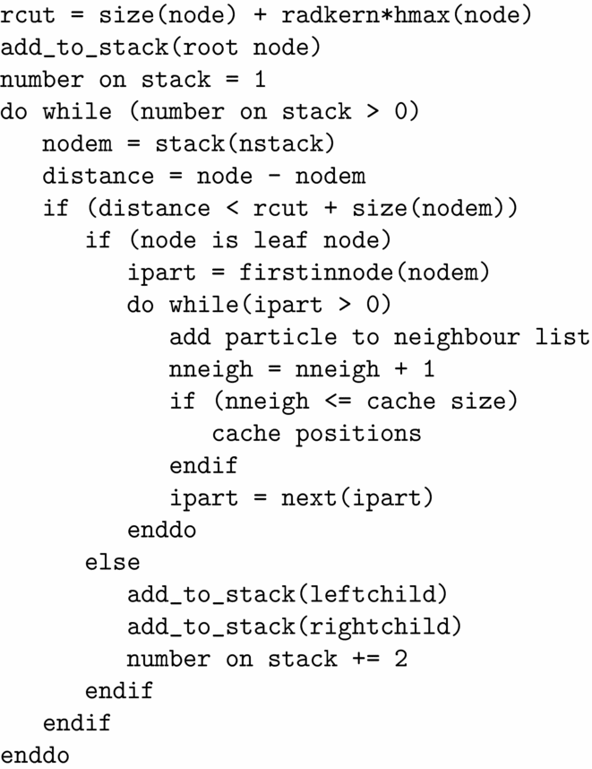
A.3.3 Density and force calculation
Once the neighbour list has been obtained for a given leaf node, we proceed to perform density iterations for each member particle. The neighbours only have to be re-cached if the smoothing length of a given particle exceeds h max for the node, which is sufficiently rare so as not to influence the code performance significantly. In the original version of Phantom (on the nogravity branch), this neighbour cache was re-used immediately for the force calculation but this is no longer the case on the master branch (see Section A.3.4). Figure A4 summarises the resulting procedure for calculating the density.
Pseudo-code for the density evaluation in Phantom, showing how Equations (3)–(5) are computed. The force evaluation [evaluating Equations (34) and (35)] is similar except that get_neigh returns neighbours within the kernel radius computed with both h i and h j and there is no need to update/iterate h (see Figure A5).
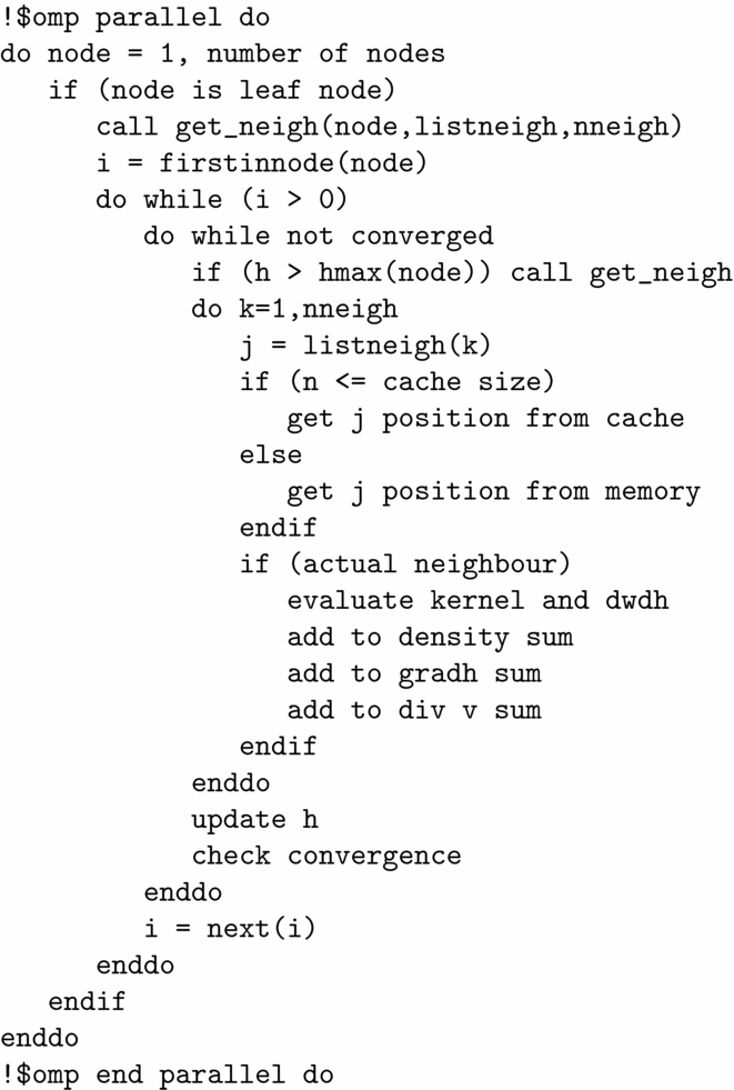
The corresponding force calculation is given in Figure A5.
Pseudo-code for the force calculation, showing how the short and long-range accelerations caused by self-gravity are computed. The quantity fnode refers to the long-range gravitational force on the node computed from interaction with distant nodes not satisfying the tree-opening criterion.
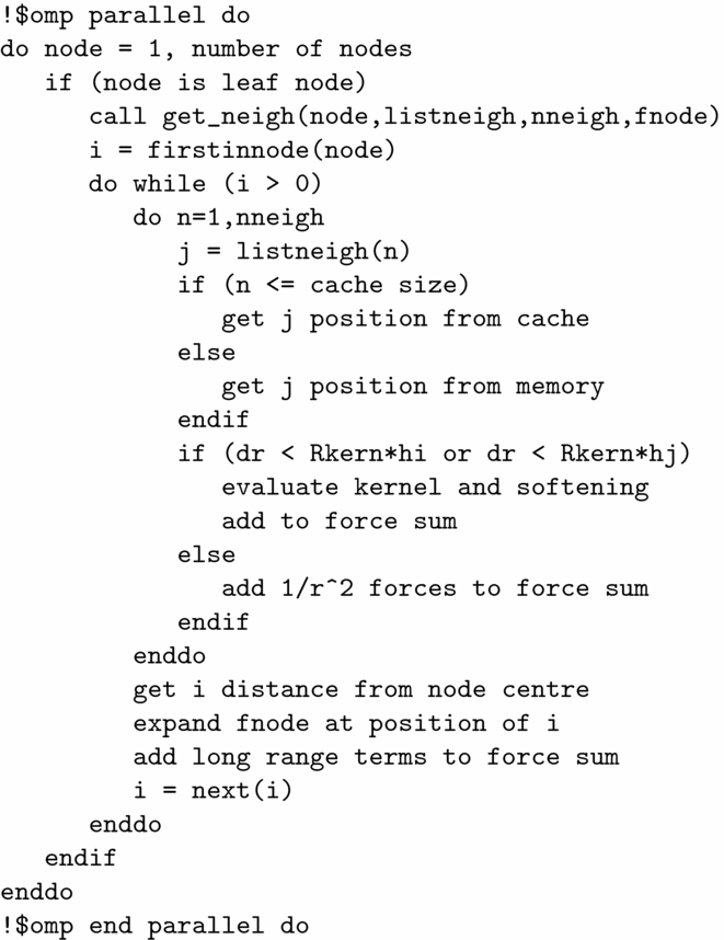
A.3.4 SPH in a single loop
A key difference in the force calculation compared to the density calculation (Section 2.1.2) is that computation of the acceleration [Equation (34)] involves searching for neighbours using both h a and h b. One may avoid this requirement, and the need to store various intermediate quantities, by noticing that the h b term can be computed by ‘giving back’ a contribution to one’s neighbours. In this way, the whole SPH algorithm can be performed in a single giant outer loop, but with multiple loops over the same set of neighbours, following the outline in Figure A4. This also greatly simplifies the neighbour search, since one can simply search for neighbours within a known search radius (2h a) without needing to search for neighbours that ‘might’ contribute if their h b is large. Hence, a simple fixed grid can be used to find neighbours, as already discussed in Section 2.1.7, and the same neighbour positions can be efficiently cached and re-used (one or more times for the density iterations, and once for the force calculation). This is the original reason we decided to average the dissipation terms as above, since at the end of the density loop one can immediately compute quantities that depend on ρa (i.e. P a and qaab) and use these to ‘give back’ the b contribution to ones neighbours. This means that the density and force calculations can be done in a single subroutine with effectively only one neighbour call, in principle, saving a factor of two in computational cost.
The two disadvantages to this approach are (i) that particles may receive simultaneous updates in a parallel calculation, requiring locking which hurts the overall scalability of the code and (ii) that when using individual timesteps only a few particles are updated at any given timestep, but with the simple neighbour search algorithms one is required to loop over all the inactive particles to see if they might contribute to an active particle. Hence, although we employed this approach for a number of years, we have now abandoned it for a more traditional approach, where the density and force calculations are done in separate subroutines and the kd-tree is used to search for neighbours checking both h a and h b for the force calculation.
A.4 OpenMP parallelisation
A.4.1 Density and force calculation
Shared memory parallelisation of the density and force calculation is described in pseudo-code in Figure A4. The parallelisation is done over the ‘leaf nodes’, each containing around 10 particles. Since the leaf nodes can be done in any order, this can be parallelised with a simple $omp parallel do statement. The neighbour search is performed once for each leaf node, so each thread must store a private cache of the neighbour list. This is not an onerous requirement, but care is required to ensure that sufficient per-thread memory is available. This usually requires setting the OMP_STACKSIZE environment variable at runtime. No thread locking is required during the density or force evaluations (unless the single loop algorithm is employed; see Section A.3.4) and the threads can be scheduled at runtime to give the best performance using either dynamic, guided or static scheduling (the default is dynamic). Static scheduling is faster when there are few density contrasts and the work per node is similar, e.g. for subsonic turbulence in a periodic box (c.f. Price Reference Price2012b).
A.4.2 Parallel tree build
We use a domain decomposition to parallelise the tree build, similar to Gafton & Rosswog (Reference Gafton and Rosswog2011). That is, we first build the tree nodes as in Figure A2, starting from the root-level node and proceeding to its children and so forth, putting each node into a queue until the number of nodes in the queue is equal to the number of OpenMP threads. Since the queue itself is executed in serial, we parallelise the loop over the particles inside the construct_node routine during the construction of each node. Once the queue is built, each thread proceeds to build its own sub-tree independently.
By default, we place each new node into a stack, so the only locking required during the build of each sub-tree is to increment the stack counter. We avoid this by adopting the indexing scheme proposed by Gafton & Rosswog (Reference Gafton and Rosswog2011) (discussed in Section 2.1.7) where the levels of the tree are stored contiguously in memory. However, to avoid excessive memory consumption, we only use this scheme while 2n level < n part. For levels deeper than this, we revert to using a stack which therefore requires a (small) critical section around the increment of the stack counter.
A.4.3 Performance
Figure A6 shows strong scaling results for the pure OpenMP code. For the scaling tests, we wanted to employ a more representative problem than the idealised tests shown in Section 5. With this in mind, we tested the scaling using a problem involving the collapse of a molecular cloud core to form a star, as described in Section 6.3. We used 106 particles in the initial sphere, corresponding to 1.44 million particles in total. We recorded the wall time of each simulation evolved for one free-fall time of the collapsing sphere, corresponding to t = 0.88 in code units.
Strong scaling results for the pure OpenMP code for the magnetised star formation problem, showing wall time as a function of the number of OpenMP threads.
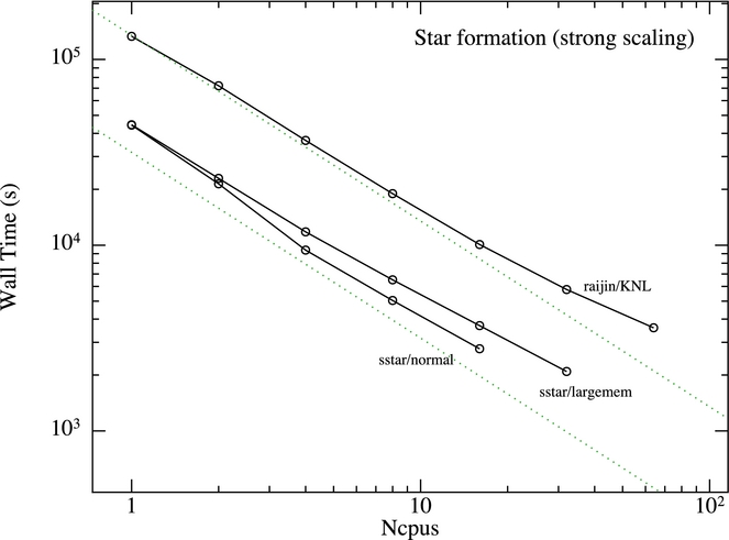
To show scaling of the OpenMP code to a reasonable number of cpus, we performed the test on the Knights Landing™ (KNL) nodes of the Raijin supercomputer (the main supercomputer of the National Computational Infrastructure in Australia). Each CPU of this machine is an Intel® Xeon Phi™ CPU 7230 with a clock speed of 1.30 GHz and a 1 024 kB cache size. The results shown in Figure A6 demonstrate strong scaling to 64 CPUs on this architecture. We used the Intel® Fortran Compiler to compile the code. Timings are also shown for the same calculation performed on two different nodes of the Swinstar supercomputer, namely the ‘largemem’ queue, consisting of up to 32 CPUs using Intel® Xeon™ E7-8837 chips running at 2.66 GHz with cache size 24 576 kB, and the ‘normal’ queue, consisting of up to 16 Intel® Xeon™ E5-2660 chips running at 2.20 GHz with cache size 20 480 kB. Our shortest wall time is achieved on the largemem queue using 32 CPUs. Figure A7 shows the corresponding speedup (wall time on single cpu divided by wall time on multiple cpus) for each architecture. We find the best scaling on the Swinstar ‘normal’ nodes, which show super-linear scaling and 100% parallel efficiency on 16 cpus. The parallel efficiency on KNL is 60% on 64 cpus.
Strong scaling results for the pure OpenMP code for the magnetised star formation problem, showing speedup as a function of the number of OpenMP threads.
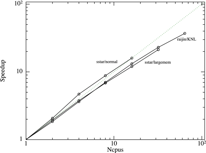
A.5 MPI parallelisation
The code has been recently parallelised for distributed memory architecture using the Message Passing Interface (MPI), using a hybrid mpi-OpenMP implementation. However, Phantom does not yet compete with gadget variants in terms of the ability to use large numbers of particles [e.g. the most recent calculations by Bocquet et al. (Reference Bocquet, Saro, Dolag and Mohr2016) employed more than 1011 particles], since almost all of our published simulations to date have been performed with the OpenMP code. Nevertheless, we describe the implementation below.
We decompose the domain using the kd-tree in a similar manner to the OpenMP parallelisation strategy described above. That is, we build a global tree from the top down until the number of tree nodes exceeds the number of MPI threads. Storing a global tree across all MPI threads is not too memory intensive since there are only as many nodes in the global tree as there are MPI threads. Each thread then proceeds to build its own independent subtree. During the neighbour search (performed for each leaf node of the tree), we then flag if a node hits parts of the tree that require remote contributions. If this is the case, we send the information for all active particles contained within the leaf node to the remote processor. Once all nodes have computed density (or force) on their local particles, they proceed to compute the contributions of local particles to the density sums of particles they have received. The results of these partial summations are then passed back to their host processors.
Particles are strictly assigned to a thread by their location in the tree. During the tree build, we exchange particles between threads to ensure that all particles are hosted by the thread allocated to their subdomain.
Within each MPI domain, the OpenMP parallelisation then operates as usual. That is, the OpenMP threads decompose the tree further into sub-trees for parallelisation.
A.6 Timestepping algorithm
When employing individual particle timesteps, we assign particles to bins numbered from zero, where zero would indicate a particle with Δt = Δt max, such that the bin identifier is
 $$\begin{equation}
i_{{\rm bin}, a} = \max \left\lbrace {\rm int}\left[\log _{2} \left(\frac{2\Delta t_{\rm max}}{\Delta t_{a}}\right) - \epsilon _{\rm tiny} \right], 0 \right\rbrace ,
\end{equation}$$
$$\begin{equation}
i_{{\rm bin}, a} = \max \left\lbrace {\rm int}\left[\log _{2} \left(\frac{2\Delta t_{\rm max}}{\Delta t_{a}}\right) - \epsilon _{\rm tiny} \right], 0 \right\rbrace ,
\end{equation}$$
where εtiny is a small number to prevent round-off error (equal to the epsilon function in Fortran). The timestep on which the particles move is simply
 $$\begin{equation}
\Delta t = \frac{{\Delta t}_{\rm max}}{2^{n_{\rm max}}},
\end{equation}$$
$$\begin{equation}
\Delta t = \frac{{\Delta t}_{\rm max}}{2^{n_{\rm max}}},
\end{equation}$$
where n max is the maximum bin identifier over all the particles. Each timestep increments a counter, i stepfrac, which if the timestep hierarchy remains fixed simply counts up to 2n max. If n max changes after each step, then i stepfrac is adjusted accordingly (i stepfrac = i stepfrac/2(n max, old − n max, new)). A particle is active if
 $$\begin{equation}
{\rm mod}\left[i_{\rm stepfrac}, 2^{(n_{\rm max} - i_{{\rm bin}, a})} \right] = 0.
\end{equation}$$
$$\begin{equation}
{\rm mod}\left[i_{\rm stepfrac}, 2^{(n_{\rm max} - i_{{\rm bin}, a})} \right] = 0.
\end{equation}$$
Active particles are moved onto a smaller timestep at any time (meaning any time that they are active and hence have their timesteps re-evaluated), but can only move onto a larger timestep if it is synchronised with the next-largest bin, determined by the condition
 $$\begin{equation}
{\rm mod}\left[i_{\rm stepfrac}, 2^{(n_{\rm max} - i_{{\rm bin}, a} + 1)} \right] = 0.
\end{equation}$$
$$\begin{equation}
{\rm mod}\left[i_{\rm stepfrac}, 2^{(n_{\rm max} - i_{{\rm bin}, a} + 1)} \right] = 0.
\end{equation}$$
In keeping with the above, particles are only allowed to move to a larger timestep by one bin at any given time.
We interpolate the positions of inactive particles by keeping all particles synchronised in time at the beginning and end of the timestep routine. This is achieved by storing an additional variable per particle, t was. All particles begin the calculation with t was set to half of their initial timestep, that is
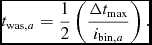 $$\begin{equation}
t_{{\rm was}, a} = \frac{1}{2} \left(\frac{\Delta t_{\rm max}}{i_{{\rm bin}, a}}\right).
\end{equation}$$
$$\begin{equation}
t_{{\rm was}, a} = \frac{1}{2} \left(\frac{\Delta t_{\rm max}}{i_{{\rm bin}, a}}\right).
\end{equation}$$
To be consistent with the RESPA algorithm (Section 2.3.3), we first update all particles to their half timestep. These velocities are then used to move the particle positions according to the inner loop of the RESPA algorithm [Equations (80)–(83)]. We then interpolate all velocities to the current time in order to evaluate the SPH derivative, finishing with the Leapfrog corrector step. Figure A8 shows the resulting pseudo-code for the entire timestepping procedure.
Pseudo-code for the timestepping routine, showing how the interaction between individual timestepping and the RESPA algorithm is implemented. External forces and sink–gas interactions are computed on the fastest timescale Δt short ≡ Δt ext. Additional quantities defined on the particles follow the velocity terms. The variable t was stores the last time the particle was active and is used to interpolate and synchronise the velocities at the beginning and end of each timestep.
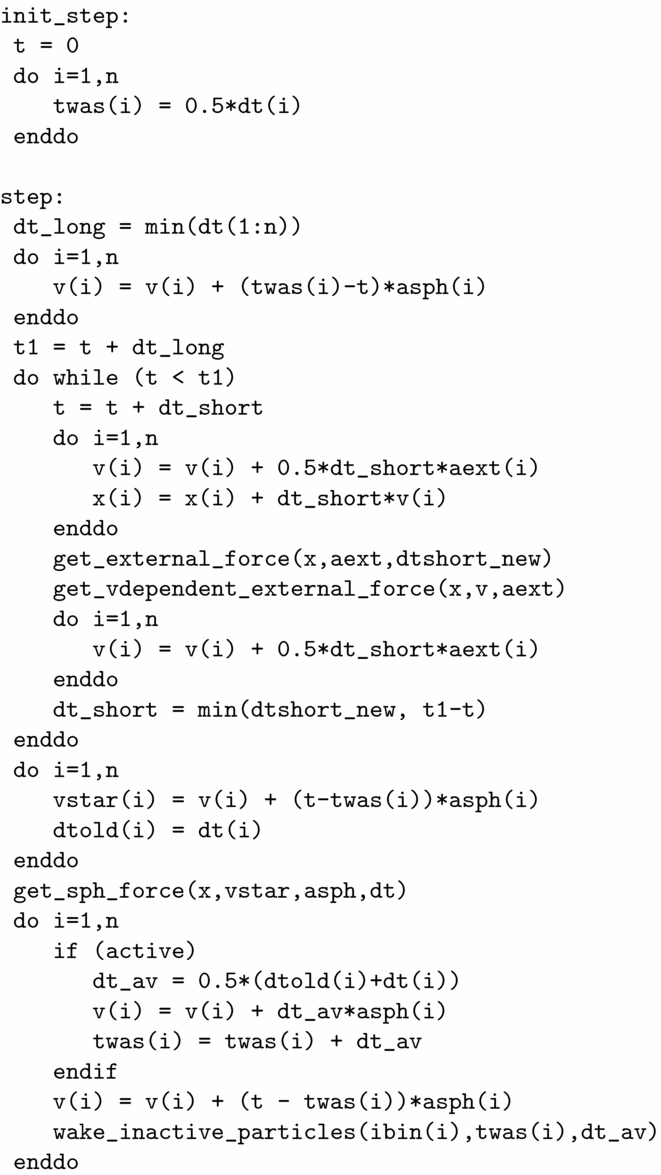
In particular, the first and last steps in the above (involving twas) interpolate the velocity to the current time. All other variables defined on the particles, including the thermal energy, magnetic field, and dust fraction, are timestepped following the velocity field.
To prevent scenarios were active particles quickly flow into an inactive region (e.g. the Sedov blast wave; see Section 5.1.3), inactive particles can be woken at any time. On each step, particles who should be woken up will be identified by comparing the ibin(i) of the active particles to ibin(j) of all i’s neighbours, both active and inactive. If ibin(i)+1 > ibin(j), then j will be woken up to ensure that its timestep is within a factor of two of its neighbours. At the end of the step, these particles will have their ibin(j) adjusted as required, and their twas(j) will be reset to the value of a particle with i bin that has perpetually been evolved on that timestep. Finally, the predicted timestep will be replaced with dt_av=dt_evolved(j)+0.5dt(j), where dt_evolved(j) is the time between the current time and the time the particle was last active, and dt(j) is the particle’s new timestep.
A.7 Initial conditions: Monte Carlo particle placement
For setting up the surface density profile in discs, we use a Monte Carlo particle placement (Section 3.3.1). This is implemented as follows: We first choose the azimuthal angle as a uniform random deviate u 1 ∈ [ϕmin, ϕmax] (0 → 2π by default). We then construct a power-law surface density profile Σ∝R −p using the rejection method, choosing a sequence of random numbers u 2 ∈ [0, f max] and iterating until we find a random number that satisfies
 $$\begin{equation}
u_{2} < f,
\end{equation}$$
$$\begin{equation}
u_{2} < f,
\end{equation}$$
where f ≡ RΣ = R 1 − p and f max = R 1 − pin (or f max = R 1 − pout if p ⩽ 1). Finally, the z position is chosen with a third random number u 3 ∈ [− z max, z max] such that u 3 < g, where g = exp[ − z 2/(2H 2)] and 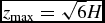 $z_{\rm max} = \sqrt{6}H$.
A.8 Runtime parameters in Phantom in relation to this paper
Table A2 lists a dictionary of compile time and run time parameters used in the code in relation to the notation used in this paper.
Various runtime parameters in the code and their relation to this paper.
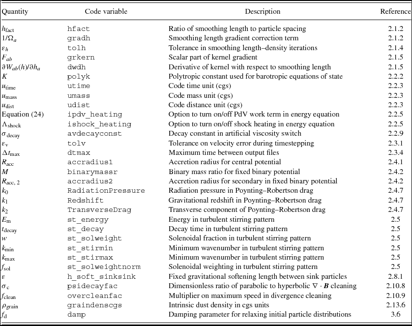
A.9 The Phantom testsuite
Most numerical codes in astrophysics are tested entirely by their performance on physical problems with known solutions, with solutions that can be compared with other codes and by maintenance of various conservation properties at run time (see Section 5). We also unit test code modules. This allows issues to be identified at a much earlier stage in development. The tests are wrapped into the nightly testsuite. When a bug that escapes the testsuite has been discovered, we have endeavoured to create a unit test to prevent a future recurrence.
A.9.1 Unit tests of derivative evaluations
The unit test of the density and force calculations checks that various derivatives evaluate to within some tolerance of the expected value. To achieve this, the test sets up 100 × 100 × 100 SPH particles in a periodic, unit cube, and specifies the input variables in terms of known functions. For example, the evaluation of the pressure gradient is checked by setting the thermal energy of each particle according to
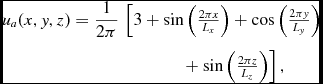 $$\begin{eqnarray}
u_{a}(x,y,z) = \frac{1}{2\pi } & \left[ 3 + \sin \left( \frac{2\pi x}{L_{x}}\right) + \cos \left( \frac{2\pi y}{L_{y}}\right) \right. \nonumber \\
& \left. \phantom{+} + \sin \left(\frac{2\pi z}{L_{z}}\right) \right],
\end{eqnarray}$$
$$\begin{eqnarray}
u_{a}(x,y,z) = \frac{1}{2\pi } & \left[ 3 + \sin \left( \frac{2\pi x}{L_{x}}\right) + \cos \left( \frac{2\pi y}{L_{y}}\right) \right. \nonumber \\
& \left. \phantom{+} + \sin \left(\frac{2\pi z}{L_{z}}\right) \right],
\end{eqnarray}$$
where L x, L y, and L z are the length of the domain in each direction and the positions are relative to the edge of the box. We then compute the acceleration according to (34) with the artificial viscosity and other terms switched off, assuming an adiabatic EOS [Equation (25)] with ρ = constant. We then test that numerical acceleration on all 106 particles is within some tolerance of the analytic pressure gradient expected from (341), namely
 $$\begin{equation}
-\frac{\nabla P_{a}}{\rho _{a}} (x,y,z) = -(\gamma - 1) \nabla u_{a}(x,y,z),
\end{equation}$$
$$\begin{equation}
-\frac{\nabla P_{a}}{\rho _{a}} (x,y,z) = -(\gamma - 1) \nabla u_{a}(x,y,z),
\end{equation}$$
where typically we use a tolerance of 10−3 in the relative error E(x) = |x − x exact|/x exact.
This procedure is repeated for the various derivatives of velocity, including the velocity divergence, curl, and all components of the strain tensor. We also test the artificial viscosity terms this way—checking that they translate correctly according to (119)—as well as the magnetic field derivatives and time derivatives, magnetic forces, artificial resistivity terms, physical viscosity terms, time derivatives of the dust fraction, and the time derivative of the velocity divergence required in the viscosity switch. We perform each of these tests also for the case where derivatives are evaluated on only a subset of the particles, as occurs when individual particle timesteps are employed.
We additionally check that various conservation properties are maintained. For example, energy conservation for hydrodynamics requires (37) to be satisfied. Hence, we include a test that checks that this summation is zero to machine precision. Similar tests are performed for magnetic fields, and for subsets of the forces that balance subsets of the thermal energy derivatives (e.g. the artificial viscosity terms).
A.9.2 Unit tests of sink particles
Unit tests for sink particles include (i) integrating a sink particle binary for 1 000 orbits and checking that this conserves total energy to a relative error of 10−6 and linear and angular momentum to machine precision; (ii) setting up a circumbinary disc of gas particles evolved for a few orbits to check that linear and angular momentum and energy are conserved; (iii) checking that circular orbits are correct in the presence of sink-sink softening; (iv) checking that accreting a gas particle onto a sink particle conserves linear and angular momentum, and that the resulting centre of mass position, velocity, and acceleration are set correctly (c.f. Section 2.8.2); and (v) checking that sink particle creation from a uniform sphere of gas particles (Section 2.8.4) succeeds and that the procedure conserves linear and angular momentum.
A.9.3 Unit tests of external forces
For external forces, we implement general tests that can be applied to any implemented external potential: (i) we check that the acceleration is the gradient of the potential by comparing a finite difference derivative of the potential, Φ, in each direction to the acceleration returned by the external force routine; and (ii) we check that the routines to solve matrix equations for velocity-dependent forces (e.g. Sections 2.4.5–2.4.7) agree with an iterative solution to the Leapfrog corrector step [Equation (69)].
A.9.4 Unit tests of neighbour finding routines
In order to unit test the neighbour finding modules (Section 2.1.7), we set up particles in a uniform random distribution with randomly assigned smoothing lengths. We then check that the neighbour list computed with the treecode agrees with a brute-force evaluation of actual neighbours. We also perform several sanity checks (i) that no dead or accreted particles appear in the neighbour list; (ii) that all particles can be reached by traversing the tree or link list structure; (iii) that nodes tagged as active contain at least one active particle and conversely that (iv) inactive cells contain only inactive particles; (v) that there is no double counting of neighbours in the neighbour lists; and (vi) that the cached and uncached neighbour lists are identical. We further check that particle neighbours are found correctly in pathological configurations, e.g. when all particles lie in a 1D line along each of the coordinate axes.
A.9.5 Unit tests of timestepping and periodic boundaries
As a simple unit test of both the timestepping and periodic boundaries, we set up 50 × 50 × 50 particles in a uniform periodic box with a constant velocity (v x = v y = v z = 1) along the box diagonal. We then evolve this for 10 timesteps and check that the density on each particle remains constant and that the acceleration and other time derivatives remain zero to machine precision.
A.9.6 Unit tests of file read/write
We check that variables written to the header of the (binary) output files are successfully recovered by the corresponding read routine, and similarly for the particle arrays written to the body of the file. This quickly and easily picks up mistakes made in reading/writing variables from/to the output file.
A.9.7 Unit tests of kernel module
We ensure that calls to different kernel routines return the same answer, and check that gradients of the kernel and kernel softening functions returned by the routines are within some small tolerance of a finite difference evaluation of these gradients.
A.9.8 Unit tests of self-gravity routines
In order to unit test the treecode self-gravity computation (Section 2.12), we (i) check that the Taylor series expansion of the force on each leaf node matches the exact force for a particle placed close to the node centre; (ii) that the Taylor series expansion of the force and potential around the distant node are within a small (~10−5) tolerance of the exact values; (iii) that the combined expansion about both the local and distant nodes produces a force within a small tolerance of the exact value; and finally (iv) that the gravitational force computed on the tree for a uniform sphere of particles is within a small tolerance (~10−3) of the force computed by direct summation.
A.9.9 Unit tests of dust physics
We unit test the dust modules by first performing sanity checks of the dust–gas drag routine—namely that the transition between Stokes and Epstein drag is continuous and that the initialisation routine completes without error. We then perform a low-resolution dustybox test (Section 5.9.1), checking the solution matches the analytic solution as in Figure 46. For one-fluid dust, we perform a low-resolution version of the dust diffusion test (Section 5.9.3), checking against the solution at every timestep is within a small tolerance of the analytic solution. Dust mass, gas mass, and energy conservation in the one-fluid dust derivatives are also checked automatically.
A.9.10 Unit tests of non-ideal MHD
We perform three unit tests on non-ideal MHD. The first is the wave damping test (see Section 5.7.1). This test also uses the super-timestepping algorithm to verify the diffusive [Equation (202) but considering only Ohmic resistivity and ambipolar diffusion] and minimum stable timesteps [Equation (72)], but then evolves the system on the smallest of the two timesteps. The second test is the standing shock test (see Section 5.7.2). This test is also designed as a secondary check on boundary particles. Both tests used fixed coefficients for the non-ideal terms, and for speed, both tests are performed at much lower resolutions than presented in the paper. The third test self-consistently calculates the non-ideal coefficients for given gas properties.
A.9.11 Other unit tests
Various other unit tests are employed, including sanity checks of individual timestepping utility routines, checking that the barotropic EOS is continuous, of the Coriolis and centrifugal force routines, checks of conservation in the generalised Newtonian potential (Section 2.4.6), of the routine to revise the tree, and of the fast inverse square root routines.
A.9.12 Sedov unit test
As a final ‘real’ unit test, the code performs a low-resolution (163) version of the Sedov blast wave test (Section 5.1.3). We check that energy and momentum are conserved at a precision appropriate to the timestepping algorithm (for global timesteps, this means momentum conservation to machine precision and energy conservation to ΔE/E 0 < 5 × 10⁻⁴; for individual timesteps, we ensure linear momentum conservation to 2 × 10⁻⁴ and energy conservation to 2 × 10⁻²).