





1. Introduction
The study of Antarctic sea ice has received increasing attention due to its pivotal role in the climate system and its susceptibility to climate change (Greenwood, Reference Greenwood2017; Turner and others, Reference Turner2022). At the same time, scientific research activities have continued in the Southern Ocean and Antarctic continent (Turner and Comiso, Reference Turner and Comiso2017). Tourism in the austral summer around Antarctica has grown rapidly (Ordoñez and others, Reference Ordoñez, Bitz and Blanchard-Wrigglesworth2018). Thus, predicting complex dynamics and behaviors of Antarctic sea ice on daily to seasonal time scales (Jung and others, Reference Jung2016), and, by extension, understanding the predictability of Antarctic sea ice, is critical for stakeholders.
Scientific communities have made some efforts to employ advanced statistical methods and numerical models to predict Antarctic sea ice and understand its predictive skill. Chen and Yuan (Reference Chen and Yuan2004) used a linear Markov model to predict seasonal Antarctic sea-ice concentration (SIC), which shows a reasonable forecast for winter sea ice in the eastern Pacific and western Atlantic sectors for 1 year in advance. Using a global climate model, Holland and others (Reference Holland, Blanchard-Wrigglesworth, Kay and Vavrus2013) assessed the influence of initial state on Antarctic sea-ice predictability. They noticed skillful prediction at the sea-ice edge zone for the lead time of 3 months, which is associated with eastward advection of anomalies in some regions. The multi-model ensemble seasonal prediction experiment also showed that the initial ocean conditions are important for Antarctic sea-ice prediction (Guemas and others, Reference Guemas, Chevallier, Déqué, Bellprat and Doblas-Reyes2016). Marchi and others (Reference Marchi2019) further identified high (low) winter (summer) predictive skill at the ice edge location in additional global coupled models and suggested that the reemergence of winter-to-winter predictability is associated with the ocean processes. Yang and others (Reference Yang, Liu, Hu, Horton, Chen and Cheng2016) pointed out that most CMIP5 models have insufficient skill to predict Antarctic sea-ice extent (SIE) on longer time scales, though certain predictability is found in the northern Ross Sea and most of the Weddell Sea associated with the ENSO teleconnection. In 2017, the Sea Ice Prediction Network South (SIPN-South) project was initiated for predicting the February Antarctic SIE (seasonal minimum). The first analysis (Massonnet and others, Reference Massonnet2018) of SIPN-South showed large errors for some predictions, low predictive skill in the Ross Sea and the possibility of systematic deficiency resulting in the delayed seasonal minimum in the predictions. Massonnet and others (Reference Massonnet, Reid, Lieser, Bitz, Fyfe and Hobbs2019) emphasized the importance of capturing weather uncertainty over the Southern Ocean. In recent years, the forecast contributed to SIPN-South can simulate the sign of anomalies on a seasonal time scale, but for some years, the median sea-ice predictions deviate significantly from the observations (Massonnet and others, Reference Massonnet2023). More recently, the employment of deep learning in seasonal prediction of Antarctic sea ice shows some promising results (Dong and others, Reference Dong2024). The research conducted by Zampieri and others (Reference Zampieri, Goessling and Jung2019) assessed reforecast skills of subseasonal to seasonal (S2S) models for Antarctic sea-ice edge during 1999–2011. They found that the European Centre for Medium-Range Weather Forecasts (ECMWF) outperforms the climatology during the lead time of 30 days, but most S2S models tend to overestimate the extent of Antarctic sea-ice edge.
Antarctic SIE fluctuates from one year to the next. However, in recent years, the state of Antarctic sea ice has changed unexpectedly. Just 3 years after reaching the record high in 2014, SIE in 2017 plunged to the third lowest record (2.29 million km2; Parkinson, Reference Parkinson2019; Wang and others, Reference Wang2022). On 21 February 2023, Antarctic SIE reached a new record low (1.788 million km2; Liu and others, Reference Liu, Zhu and Chen2023). Moreover, the annual minimum of the Antarctic SIE during 2022–25 has been in a row below 2 million km2. Previous evaluations of S2S models’ Antarctic sea-ice prediction (Zampieri and others, Reference Zampieri, Goessling and Jung2019; Xiu and others, Reference Xiu, Luo, Yang, Tietsche, Day and Chen2022; Gao and others, Reference Gao2024) have primarily focused on their forecast skill during years without such exceptional changes. A few recent studies investigated the predictability of record-low Antarctic SIE in austral summer (Massonnet and others, Reference Massonnet2023) and winter (Espinosa and others, Reference Espinosa, Blanchard-Wrigglesworth and Bitz2024), demonstrating the critical role of pre-existing ocean heat in driving record-low events. As to yet, operational S2S models struggle to initialize these anomalies. In this study, we select four periods during 2022–23 and aim to assess the capability of current operational S2S numerical models in predicting the extremely anomalous SIE during the four periods. The scientific questions that we want to answer include:
(1) Are current S2S models skillful in predicting the exceptionally rapid decrease of Antarctic SIE that contributes to the record low seasonal minimum in February 2023?
(2) To what extent can current S2S models capture the exceptionally slow growth of Antarctic SIE that partly contributed to the record low seasonal maximum in September 2023?
2. Data and methods
2.1. Data
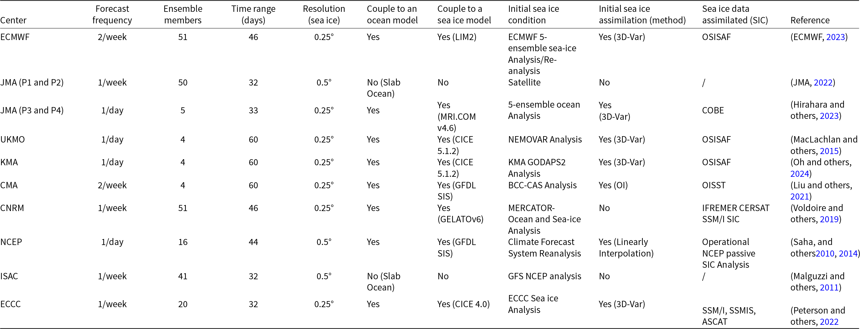
The S2S prediction project plays a vital role in bridging the gap between weather forecasts and seasonal climate predictions (Woolnough and others, Reference Woolnough2024), offering a unique perspective for this assessment. The S2S archive provides near-real-time and re-forecast ensemble forecasts for a period of 30 up to 62 days (Vitart and others, Reference Vitart2017). The variable used here is the daily-averaged SIC from the near-real-time ensemble forecast. The forecast centers and their models considered here include the ECMWF, the Japan Meteorological Agency (JMA), the UK Met Office (UKMO), the Korea Meteorological Administration (KMA), the China Meteorological Administration (CMA), the Météo-France/Centre national de recherche météorologiques (CNRM), the National Centers for Environmental Prediction (NCEP), the Institute of Atmospheric Sciences and Climate (ISAC) and the Environment and Climate Change Canada (ECCC). Since these forecast centers have different model settings (Vitart and others, Reference Vitart2017), we summarize their forecast duration, number of ensemble members, forecast frequency, model coupling and method of data assimilation in Table 1 to facilitate comparison. In this study, we focus on their predictive skill for Antarctic SIE during four 46 day periods (Fig. S1). One period is featured with exceptionally rapid decrease of Antarctic SIE from 17 November 2022 to 1 January 2023 (hereafter referred to as P1), and one period of sustained low SIE from 5 December 2022 to 19 January 2023 (hereafter referred to as P2), both P1 and P2 led to the record seasonal minimum in February 2023. The other periods are characterized by exceptionally slow growth from 6 April 2023 to 21 May 2023 (hereafter referred to as P3) and 18 May 2023 to 2 July 2023 (hereafter referred to as P4), which partly contributed to the record low of seasonal maximum in September 2023. The prediction results of these different forecast systems are archived with a horizontal resolution of 1.5° × 1.5° by ECMWF and CMA.
Features of the S2S models used in this study. JMA has upgraded between 2022 and 2023.

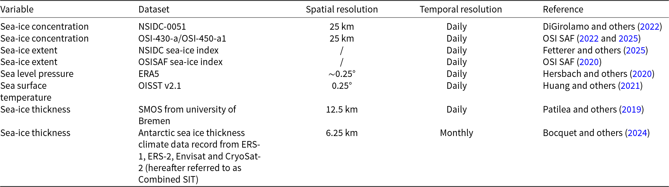
Table 2 shows all the observational and reanalysis datasets used in this study. For satellite-derived Antarctic sea-ice data, we use the daily SIC products from multiple sources. One primary dataset is from the National Snow and Ice Data Center (NSIDC), derived from the Special Sensor Microwave Imager/Sounder (SSMIS) and mapped on a 25 km × 25 km polar stereographic grid. The other is the OSI SAF climate sea-ice analysis product (OSI-430-a [OSI SAF, 2022] and OSI-450-a1 [OSI SAF, 2025]) produced by the EUMETSAT Ocean and Sea Ice Satellite Application Facility (OSISAF). Daily sea level pressure (SLP) from the European Center for Medium-Range Weather Forecasts Reanalysis (Hersbach and others, Reference Hersbach2020) and the Optimum Interpolation Sea Surface Temperature version 2.1 (OISST; Huang and others, Reference Huang2021) is also used to facilitate the assessment. We use two sea-ice thickness (SIT) products to discuss the limitations of S2S models’ SIT, and they are daily SIT from the University of Bremen (Patilea and others, Reference Patilea, Heygster, Huntemann and Spreen2019) and monthly SIT climate data record from ERS-1, ERS-2, Envisat and CryoSat-2 (Bocquet and others, Reference Bocquet, Fleury, Rémy and Piras2024).
Summary of observational and reanalysis datasets used in this study.

2.2. Methods
To better illustrate the short-term evolution of SIE anomaly relative to its climatological mean, we computed the 15 day cumulative anomaly for each day over the following 15 days from September 2022 to September 2023. As shown in Fig. S1, the blue bars indicate these cumulative anomalies. Pronounced quick increases are evident in P1 and P2 during the melting season and in P3 and P4 during the growing season. Based on this analysis and considering the varying initialization dates of the S2S models, we selected these four representative periods for evaluations.
To evaluate the predictive skill of Antarctic SIE during the aforementioned four key periods, we compare Antarctic SIE predictions with two benchmark methods. One is the climatology prediction based on the average of Antarctic SIE during 1991–2020 (hereafter referred to as CLIM). The other is the damped anomaly persistence prediction (hereafter referred to as DAMP, Van Den Dool, Reference Van Den Dool2006). DAMP is defined as follows:
 \begin{equation}\begin{array}{*{20}{c}}
{{\text{SI}}{{\text{E}}_{{\text{damp}}}}\left( t \right) = {\text{SI}}{{\text{E}}_{{\text{clim}}}}\left( t \right) + {\text{SI}}{{\text{E}}_{{\text{anom}}}}\left( 0 \right) \times A\left( t \right) \times \frac{{\sigma \left( t \right)}}{{\sigma \left( 0 \right)}}}
\end{array}\end{equation}
\begin{equation}\begin{array}{*{20}{c}}
{{\text{SI}}{{\text{E}}_{{\text{damp}}}}\left( t \right) = {\text{SI}}{{\text{E}}_{{\text{clim}}}}\left( t \right) + {\text{SI}}{{\text{E}}_{{\text{anom}}}}\left( 0 \right) \times A\left( t \right) \times \frac{{\sigma \left( t \right)}}{{\sigma \left( 0 \right)}}}
\end{array}\end{equation} where  $SI{E_{clim}}\left( t \right){ }$ is climatological SIE for day t based on the 1991–2020 average,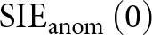 ${\text{SI}}{{\text{E}}_{{\text{anom}}}}\left( 0 \right)$ is the SIE anomaly on the initial day (day 0), $A\left( t \right){ }$ is the lag-t autocorrelation of the daily CLIM-SIE time series over 1991–2020, $\sigma \left( 0 \right){ }$ and $\sigma \left( t \right){ }$ are the standard deviation of CLIM-SIE values across all years at lag 0 and lag t and $\frac{{\sigma \left( t \right)}}{{\sigma \left( 0 \right)}}$ is the daily standard deviation ratio. DAMP combines the SIE climatology at lag t with present and persisted SIE anomaly to estimate future SIE condition (Wang and others, Reference Wang, Yuan and Li2019; Yang and others, Reference Yang, Liu and Xu2020; Niraula and Goessling, Reference Niraula and Goessling2021). Antarctic SIE is calculated as the total area of grids where SIC is greater than 15%. We also compare the deviation of the observed or predicted Antarctic SIE from the climatological value. For the two periods, the observed deviations are consistently negative. Thus, if the deviation of S2S forecast is larger than the observed deviation, it suggests a slower decline (faster growth) of SIE during P1 and P2 (P3 and P4). To better evaluate the impact of Antarctic sea-ice data assimilated by S2S forecast systems on subsequent prediction, we also present the predictions starting from different forecast dates and corresponding DAMP predictions.
To evaluate the predictive skill of Antarctic sea-ice edge, we use the integrated ice edge error (IIEE; Goessling and others, Reference Goessling, Tietsche, Day, Hawkins and Jung2016). The IIEE represents the total area of discrepancy between forecasted and observed regions where ice concentration either exceeds or falls below the 15% threshold. This metric quantifies the spatial mismatch by calculating the symmetric difference between the predicted ice edge boundary and the actual ice extent, which is the sum of overestimated error (OE) and underestimated error (UE), with its mathematical formulation expressed as:
 \begin{equation}\begin{array}{*{20}{c}}
{{\text{IIEE}} = {\text{OE}} + {\text{UE}}}
\end{array}\end{equation}
\begin{equation}\begin{array}{*{20}{c}}
{{\text{IIEE}} = {\text{OE}} + {\text{UE}}}
\end{array}\end{equation} \begin{equation}
{\text{OE}} = {\int_{A}} \max \left(c_{\text{p}} - {c_{\text{o}}}\right) \, dA
\end{equation}
\begin{equation}
{\text{OE}} = {\int_{A}} \max \left(c_{\text{p}} - {c_{\text{o}}}\right) \, dA
\end{equation} \begin{equation}
\text{UE} = {\int_{A}} \max \left(c_{o} - c_{p} \right) \, dA
\end{equation}
\begin{equation}
\text{UE} = {\int_{A}} \max \left(c_{o} - c_{p} \right) \, dA
\end{equation} where  $A$ is the grid-cell area, $c$ = 1 where the SIC $ \geqslant $15% and $c$ = 0 elsewhere. The subscripts ${\text{p}}$ and ${\text{o}}$ denote the prediction and the verifying analysis (NSIDC-0051 or OSI-430-a/OSI-450-a1). The IIEE of climatological forecast benchmark is calculated based on the median SIC (1991–2020) for each grid cell (Goessling and Jung, Reference Goessling and Jung2018). On this basis, the IIEE of DAMP is obtained by applying the ${\text{SI}}{{\text{E}}_{{\text{damp}}}}$ calculation formula to the grid-point SIC using the median climatological SIC as climatological reference.
In this study, within the zonal band of the low-pressure center identified for each period, the SLP gradient is calculated as the minimum SLP minus the averaged SLP. The minimum SLP is defined as the lowest SLP values of the S2S ensemble mean and ERA5, and the averaged SLP is defined as the regional averaged SLP of the S2S ensemble mean and that of ERA5. This approach allows us to qualitatively compare the extent to which the simulated pressure gradient deviates from the reanalysis within the low-pressure system. As shown in the results section (Figs 4 and 8), the cumulative SIE bias does increase with the SLP gradient bias, though the number of the S2S models is small. More models may be needed to achieve significant correlations.
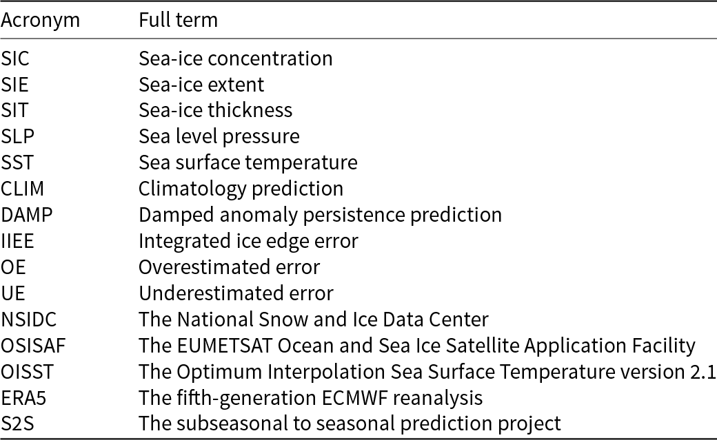
In this study, all acronyms and abbreviations used in the manuscript are summarized in Table 3 for clarity and ease of reference.
List of acronyms and abbreviations used in this study.

3. Results
3.1. Exceptionally rapid decrease of Antarctic SIE (P1 and P2)
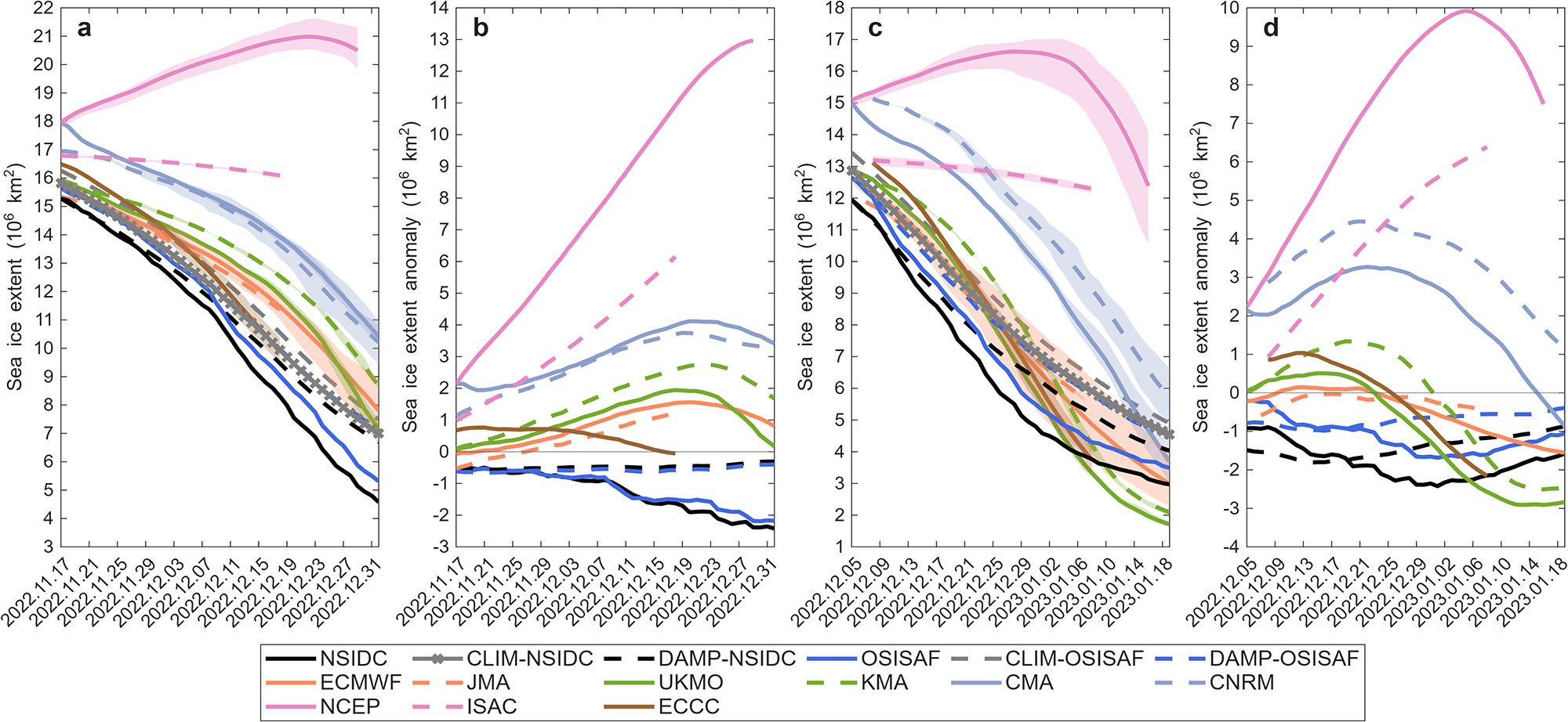
Figure 1 shows the evolution of the predicted Antarctic SIE by S2S models and two benchmark methods, as well as their differences relative to the NSIDC climatology during P1. At the initial day, the observed SIE of NSIDC is 0.54 × 10⁶ km2 (OSISAF is 0.61 × 10⁶ km2) less than their climatology (Fig. 1a). The biases of ice extent between each verifying sea-ice dataset (hereafter referred to as observational SIE or observation) and their CLIM continue to increase, reaching its maximum on day 46, finally about 2.42 × 10⁶ km2 of NSIDC and 2.19 × 10⁶ km2 of OSISAF (Fig. 1b). This made that Antarctic SIE in December 2022 stood at the lowest in the 45 year satellite observation. The initial SIE bias of the S2S model is relatively large. Except for JMA, all models overestimate the initial SIE relative to the NSIDC analysis, with a range of up to 2.69 × 10⁶ km2. Among them, the biases of CMA, CNRM, NCEP and ISAC are significantly greater than CLIM, while the biases of ECMWF, UKMO and KMA are basically consistent with CLIM. JMA is closest to the NSIDC analysis, while ECMWF, UKMO and KMA are more consistent with the OSISAF analysis. The spatial distribution of SIC indicates that larger initial SIE in the CMA, CNRM, NCEP and ISAC models is significantly overestimated, mainly due to overestimation of the ice cover in the central and eastern Pacific, Atlantic and western Indian Oceans (Fig. S2). As suggested in Table 1, the initial model-observation SIE discrepancies are related to differences in (1) modeled SIC, (2) sources of SIC assimilated and (3) data assimilation methods to combine (1) and (2). For example, the initial SIE difference between ECMWF, UKMO and KMA and the observation is largely due to the difference in their simulated sea-ice state, given that they all utilize 3D-Var to assimilate the observed ice concentration developed by OSISAF.
(a) Predicted and observed Antarctic SIE during P1. (b) Differences in SIE between predictions, verifying sea-ice analyses and climatology during P1. (c, d) Same as (a, b), but for P2. Colored lines denote different S2S models, with shaded areas indicating the ensemble spread and solid lines representing the ensemble mean. In (b) and (d), S2S anomalies are relative to CLIM-NSIDC, while OSISAF and DAMP-OSISAF anomalies are relative to CLIM-OSISAF.

Regarding predictions, all S2S models predict a decrease of SIE during P1, except that (1) NCEP simulates an increase of SIE for ∼5 weeks, followed by a slow decrease, and (2) the SIE predicted by ISAC is almost stable throughout the period (Fig. 1a). The lack of forecast skill for ISAC largely due to that ISAC is not coupled to a sea-ice model, in which sea-ice state is held fixed if sea-ice fraction is above (below) the climatology in the season of fall–winter (spring–summer) and is relaxed to the climatology otherwise (Malguzzi and others, Reference Malguzzi, Buzzi and Drofa2011). Furthermore, compared to observations, all models overestimated SIE for most of P1. This is partly related to the above initial positive SIE biases. Except for ECCC, which simulates a decline rate comparable to the observations, none of the other models can predict the observed accelerated decline during December 2022. In fact, most models either follow the pace of or even melt much slower than the climatological evolution (Fig. 1b). This suggests that model physics in current numerical weather prediction models might not adapt to the exceptionally rapid decrease of Antarctic sea ice that occurred during P1. Additionally, we note that most models simulate a much delayed very rapid decrease of SIE.
Throughout all forecast times, both baseline methods (CLIM and DAMP) of two observations overestimated SIE, particularly during the observed accelerated decline phase (Fig. 1a). Only ECCC shows a similar rate of decline to CLIM-NSIDC, while ECMWF and JMA initially approached CLIM but subsequently experienced a slower rate of decline. Therefore, none of the considered S2S models captured the anomalously rapid decline in Antarctic SIE during P1.
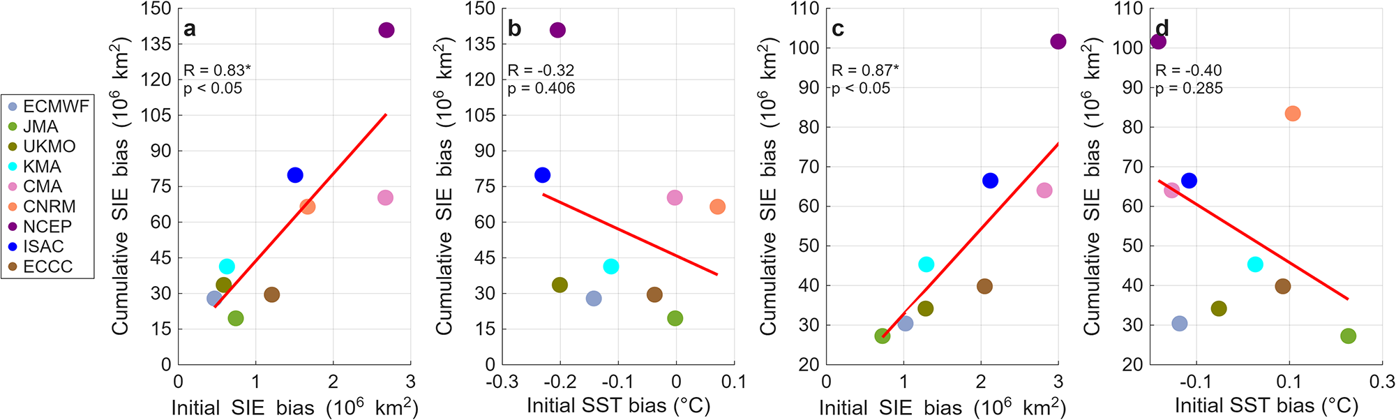
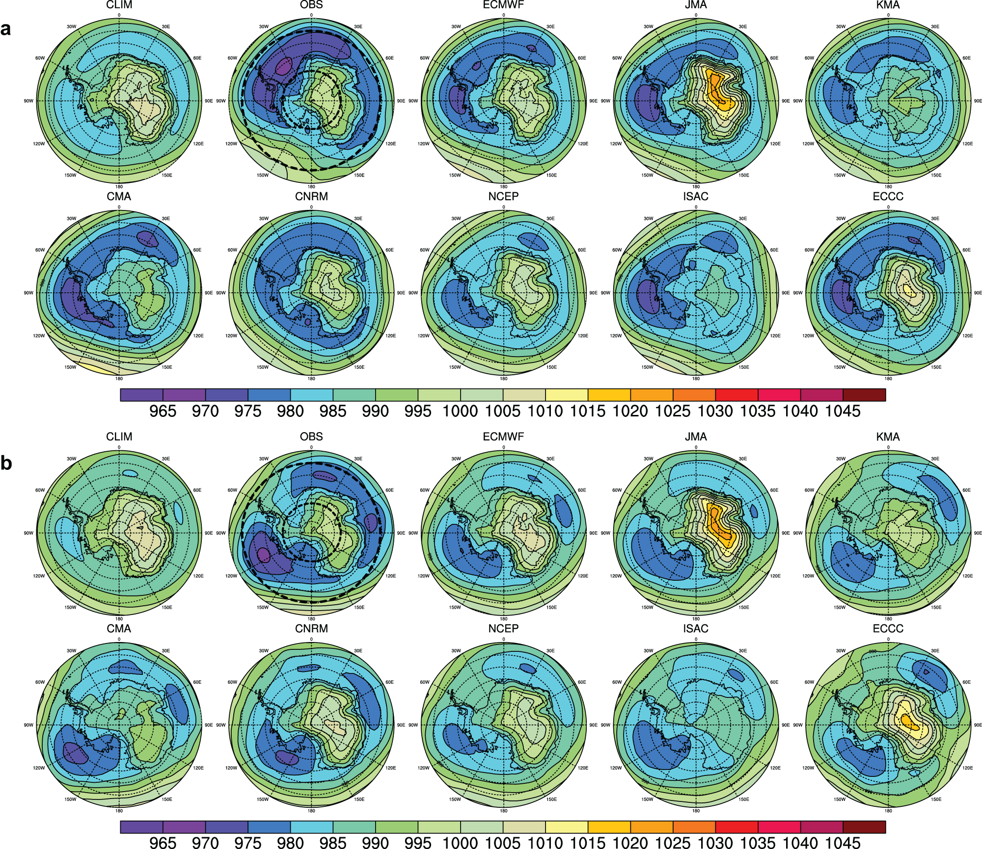
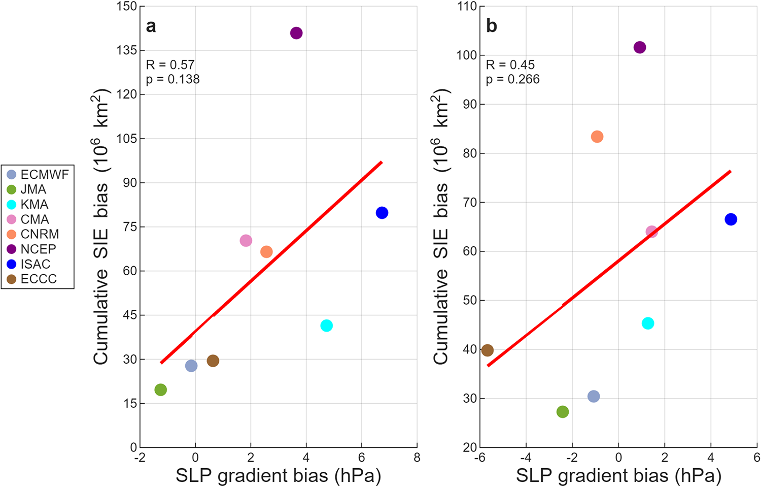
Here, we conduct further analyses to understand the factors that lead to the S2S models failing to accurately predict the observed rapid sea ice decline in P1. First, as shown in Fig. 2a, a strong positive correlation exists between the initial SIE bias and the cumulative SIE bias in the S2S models, indicating that differences present at initialization tend to persist into the forecasts, such that models initialized with a more extended sea-ice state also tend to maintain larger SIE throughout the forecast period. We note that this correlation does not necessarily imply a causal relationship between initialization errors and forecast errors but may partly reflect uncertainties in the observational analyses used both for model initialization and for forecast verification. Second, some research emphasized the importance of pre-existing ocean conditions on the following sea-ice anomaly (Purich and Doddridge, Reference Purich and Doddridge2023; Espinosa and others, Reference Espinosa, Blanchard-Wrigglesworth and Bitz2024). As shown in Fig. S3, most S2S models exhibit negative SST biases to the north of the sea-ice edge zone during P1, which encourages the growth of sea ice. The averaged SST bias shows a negative correlation with the cumulative SIE bias (Fig. 2b), suggesting that biases in upper-ocean thermal conditions present at initialization are associated with subsequent SIE evolution. As with SIE, this relationship may reflect both the influence of ocean initial conditions and the consistency between model states and the assimilated observational fields. Third, atmospheric circulation anomalies have a certain influence on Antarctic sea-ice distribution and variability of Antarctic sea ice (Fogt and others, Reference Fogt, Dalaiden and O’Connor2024). Figure 3a shows the observed and predicted SLP averaged over 21 days during the rapid decline period. The observation shows a large low-pressure belt existed over the Southern Ocean during this period, extending from the Bellingshausen Sea around West Antarctica to the Indian Ocean sector, with an unusually strong low-pressure center at the Weddell Sea. All S2S models simulate the significantly weaker low-pressure intensity and pressure gradients in the central Weddell Sea, with the low-pressure center mostly located in either the Bellingshausen or Amundsen Sea. The former reduces ice melting on the eastern side of the Weddell Sea low and ice advection on the western side. The latter increases ice advection in the eastern Amundsen Sea and western Bellingshausen Sea. This, to some extent, leads to a slowdown in the rate of sea-ice reduction in these regions and delayed the retreat of sea ice at the outer edges of the Amundsen and Bellingshausen Seas. Furthermore, the relationship between SLP gradient bias and cumulative SIE bias within the zonal low-pressure belt (Fig. 4a, R = 0.57) indicates that models with incorrect SLP gradients tend to overestimate SIE, highlighting the importance of accurate SLP prediction for sea-ice prediction.
(a) Correlations between cumulative S2S-SIE biases during days 5–25 and initial SIE bias during P1. (b) Correlations between cumulative S2S-SIE biases during days 5–25 and initial SST bias during P1. (c, d) Same as (a, b), but for P2. SIE biases are the differences between the S2S ensemble mean and NSIDC within 60° S–77° S (region selected to examine atmosphere–ocean–sea-ice interactions; see Figure 3). Initial SST biases are the differences between the S2S ensemble mean and OISST, averaged over ice-free grid points south of 55° S. Asterisks denote statistically significant correlations (p < 0.05); values without asterisks are labeled with the corresponding p-values.

Spatial distribution of SLP averaged from day 5 to day 25 during (a) P1 and (b) P2. For each period, the panels show climatology, observation and S2S model. Note that UKMO is not shown because it does not provide SLP.

Correlations between cumulative S2S-SIE biases during days 5–25 and the SLP gradient bias between S2S and ERA5 during (a) P1 and (b) P2. SIE biases are calculated in the same way as Figure 2. The SLP gradient is defined as the minimum SLP minus the averaged SLP.

Following the exceptionally rapid decline during 17 November 2022 to 1 January 2023, we further examine another period from 5 December 2022 to 19 January 2023, which also exhibits an unusually rapid decline in Antarctic SIE compared to the climatology. At the initial day of P2, the observed SIE of NSIDC is 0.92 × 10⁶ km2 (OSISAF is 0.79 × 10⁶ km2) less than their climatology (Fig. 1c). The deviation in the ice extent between two observations and their CLIM becomes larger, reaching the largest after 4 weeks, about 2.42 × 10⁶ km2 of NSIDC and 2.19 × 10⁶ km2 of OSISAF followed by very slowly reduced deviation (Fig. 1d). The initial SIE bias of the S2S models shows large spread, ranging from 0.33 to 3.79 × 10⁶ km2, which is related to the inherent uncertainty (∼1 × 10⁶ km2) between two sea-ice analyses. All the models overestimate the observed initial SIE, and CMA, CNRM and NCEP are substantially larger than the two sea-ice analyses, whereas UKMO, KMA and ECMWF are almost in line with the OSISAF. Among them, JMA is closer to the two sea-ice analyses. The spatial distribution of SIC suggests that substantially larger initial SIE in CMA, CNRM and NCEP is mainly due to great overestimation of the ice cover in the central and eastern Pacific, Atlantic and western Indian Oceans (Fig. S4). It is also noted that most models show polynyas in the Indian Ocean sector (east of the Weddell Sea) and the Amundsen Sea during P2, but the spatial scale is smaller compared to the observations.
In terms of prediction, all S2S models predict a decrease of SIE during P2, except that (1) NCEP simulates an increase of SIE for ∼3 weeks, followed by a rapid decrease, and (2) the predicted SIE of ISAC is almost level off during the entire period (Fig. 1c). Besides, all the models also overestimate the ice extent for most of P2 compared to the observations, which is partly related to the above initial positive SIE biases. Moreover, similar to P1, none of the models successfully capture the observed accelerated melting, and the timing of the rapid decrease in most S2S models remains noticeably delayed. This indicates that, despite the inclusion of initial sea-ice data assimilation, the models still struggle to reproduce the accelerated sea-ice loss that occurred from December 2022 to January 2023.
Across all forecast times, two benchmark methods (CLIM and DAMP) significantly overestimate SIE, especially starting from the observed accelerated decline (Fig. 1c). Only two models (ECMWF and JMA) show predictive skill close to the CLIM-NSIDC during the observed accelerated decline period, but unlike ECMWF (a fully coupled model), sea ice in JMA is simulated as an ice slab since its atmospheric model is not coupling to an ocean/sea-ice model. Although ECMWF, UKMO, ECCC and KMA achieve better predictive skill than the DAMP prediction near the end of P1, it is due to the erroneous delayed rapid decrease of the simulated SIE as mentioned above. Thus, all the S2S models considered do not capture the exceptionally rapid decrease of Antarctic SIE during P2.
Further analyses during P2 indicate that a strong positive correlation exists between the initial SIE bias and the cumulative SIE bias in the S2S models (Fig. 2c), indicating that differences present in the analyzed SIE at initialization tend to persist. Most S2S models exhibit negative SST biases to the north of the sea-ice edge zone during P2, similar to P1. These SST biases are associated with a tendency for the models to maintain more extensive sea ice during the forecasts, which may partly reflect consistency between the initial ocean state and the assimilated observational fields. The combination of these initial condition biases contributes to the models’ tendency to predict excessive SIE. From the perspective of synoptic atmospheric circulation during P2, the observation shows two low-pressure systems over the Southern Ocean during this period (Fig. 3b). One is an anomalously strong Amundsen Sea Low (ASL), leading to the observed large polynya extending from the eastern Bellingshausen Sea to the eastern Ross Sea. The other is a band of anomalously low pressure extending from the central Weddell Sea to the Indian Ocean. Surface pressure anomalies, particularly those associated with the ASL, can influence sea ice by altering near-surface wind patterns and thereby modifying sea-ice advection and regional melt or retreat of the ice edge (Holland and others, Reference Holland, Landrum, Raphael and Kwok2018; Wang and others, Reference Wang2023). All S2S models simulate a much weaker ASL and weaker pressure gradient in the central Weddell Sea, which is consistent with a slower simulated rate of sea-ice decrease in these regions. The former reduces ice melting to the east of ASL and ice advection to the west of ASL. The latter reduces the ice advection in the central and eastern Weddell Seas. This partly results in slower sea-ice decrease there. Further, the relationship between SLP gradient bias in a zonal low-pressure belt and cumulative SIE bias correlates positively (Fig. 4b, R = 0.45). This also indicates that models with larger positive SLP biases tend to overestimate SIE, highlighting the importance of accurate SLP prediction, especially the SLP gradient prediction during sea-ice melting.
3.2. Exceptionally slow increase of Antarctic SIE (P3 and P4)
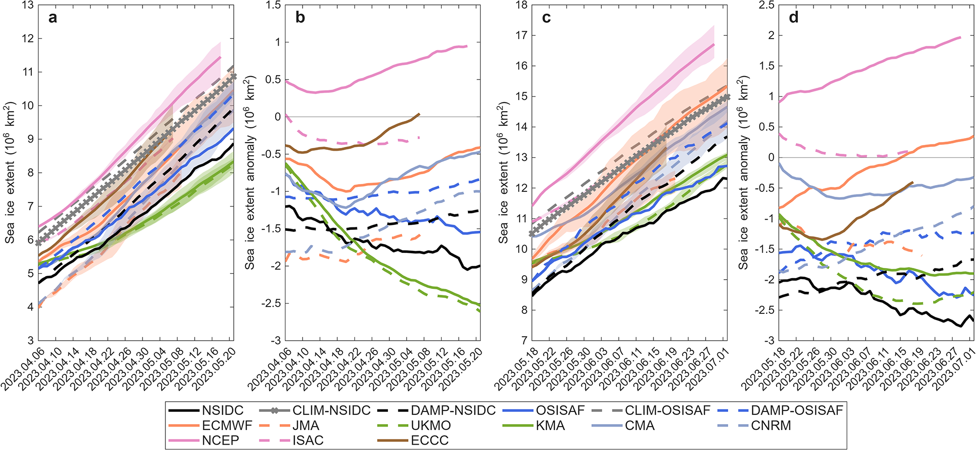
Next, we focus on the prediction by the S2S models from 6 April 2023 to 21 May 2023, an exceptionally slow recovery period compared to the climatology. At the beginning, the observed SIE of NSIDC is lower than the climatology by 1.2 × 10⁶ km2 (OSISAF is 1.07 × 10⁶ km2), and then the deviation is enlarged, reaching the largest at the end of P3 (2.05 × 10⁶ km2 of NSIDC and 1.89 × 10⁶ km2 of OSISAF, Fig. 5a), which partly contributes to the record low of seasonal maximum in 2023 since the satellite observation. The S2S models also display different initial SIE biases, ranging from −0.74 to 1.69 × 10⁶ km2, partly due to uncertainties in the sea-ice analysis (difference between OSISAF and NSIDC is about 0.4 × 10⁶ km2). NCEP has the largest positive bias, resulting from great overestimation of the ice concentration in the Pacific and Atlantic sectors (Fig. S6). ECMWF, CMA, ISAC and ECCC lie between two observations and CLIM. UKMO and KMA are close to the observation of OSISAF and larger than the observation of NSIDC. JMA and CNRM show negative biases, which is due to little sea-ice cover in the Amundsen Sea and the region extending from the Indian Ocean to the western Pacific.
(a) Predicted and observed Antarctic SIE during P3. (b) Differences in SIE between predictions, verifying sea-ice analyses and climatology during P3. (c, d) Same as (a, b), but for P4. Line styles and shading are the same as in Figure 1.

For the prediction, all S2S models predict an increase in SIE during P3. However, most models are close to the CLIM rate of increase, which overestimate the ice recovery rates compared to observations (Fig. 5b); that is, even with a large initial negative bias, the SIE of JMA and CNRM increases rapidly and approaches the observations after 3 weeks. Two models (UKMO and KMA) capture the observed anomalously slow growth, though they simulate slower growth at the beginning compared to the observations.
Similar to P1 and P2, Antarctic SIE is also significantly overestimated by two benchmark methods during P3. ECMWF and CMA have predictive skill close to the DAMP prediction. Different from P1 and P2, there are two models (UKMO and KMA) that show better skill than the DAMP prediction. It is worth noting that due to the spatial cancellation of regional errors (Fig. S6), the overall SIE bias of the CLIM and DAMP benchmarks is relatively small. When assessed by the accuracy of the ice edge location rather than total SIE, the models perform better than DAMP.
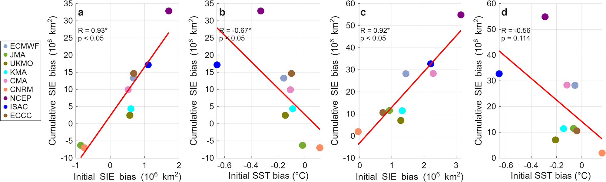
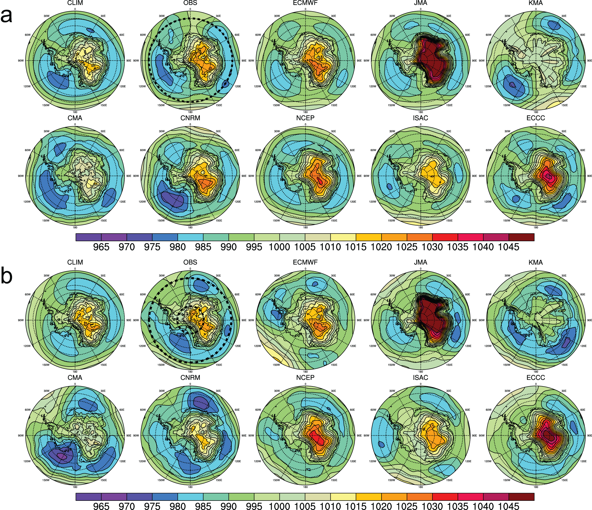
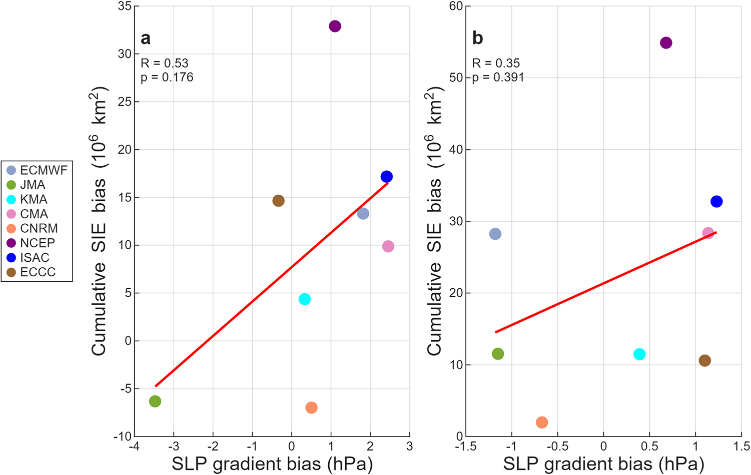
Further analyses during P3 show that the S2S models have a strong positive correlation between initial SIE bias and cumulative SIE bias (Fig. 6a). Most models exhibit negative evident SST biases to the north of the sea-ice edge zone during P3 (Fig. S7), which encourages the growth of sea ice. This is also reflected in the negative correlation between averaged SST bias and cumulative SIE bias (Fig. 6b). These relationships indicate that biases present in the initial conditions tend to be reflected in the subsequent SIE evolution. The combination of these initial condition biases contributes to the models’ tendency to predict excessive SIE. From the perspective of synoptic atmospheric circulation during P3, the observation shows two bands of low-pressure anomalies (Fig. 7a). One is extending from the eastern Pacific to the central Atlantic. This causes an unusually strong and eastward-shifted ASL. Its eastern side results in strong ice melting and advection. Thus, the Bellingshausen Sea is nearly ice-free along the entire coast, and the eastern Weddell Sea has low ice cover. The other is extending from the western Indian Ocean to the eastern Pacific, leading to anomalously low SIC along the East Antarctic coast. Except for CMA, almost all S2S models simulate either weaker ASL or low-pressure center more toward the central Pacific sector and weaker pressure gradients over the Indian Ocean. This partly results in faster sea-ice growth there. Furthermore, the SLP gradient biases within a zonally averaged low-pressure belt show a good correlation with the cumulative SIE bias (Fig. 8a, R = 0.53). Although these correlations do not reach the conventional threshold of statistical significance (p = 0.17) with the present sample size, the coherent signal reinforces the potential importance of accurately capturing pressure extremes and their gradients for improving sea-ice prediction.
(a) Correlations between cumulative S2S-SIE biases during days 5–25 and initial SIE bias during P3. (b) Correlations between cumulative S2S-SIE biases during days 5–25 and initial SST bias during P3. (c, d) Same as (a, b), but for P4. SIE biases are the differences between the S2S ensemble mean and NSIDC within 55° S–77° S for P3 and 58° S–70° S for P4 (region selected to examine atmosphere–ocean–sea-ice interactions; see Figure 7). Initial SST biases are calculated in the same way as Figure 2.

Spatial distribution of SLP averaged from day 5 to day 25 during (a) P3 and (b) P4. For each period, the panels show climatology, observation and S2S model. Note that UKMO is not shown because it does not provide SLP.

Correlations between cumulative S2S-SIE biases during days 5–25 and the SLP gradient bias between S2S and ERA5 during (a) P3 and (b) P4. SIE biases are calculated in the same way as Figure 6. The SLP gradient is defined as the minimum SLP minus the averaged SLP.

Following the exceptionally slow recovery during April–May 2023 (P3), we further examine another period from May 18 to 2 July 2023 (P4), which also exhibits an unusually slow growth in Antarctic SIE compared to the climatology. At the beginning of P4, the observed SIE remains well below the climatology, with a negative anomaly of 2.05 × 10⁶ km2 from NSIDC and 1.89 × 10⁶ km2 from OSISAF, and this anomaly persists throughout the period (Fig. 5c), reflecting the prolonged suppression of sea-ice growth during the autumn in 2023. The S2S models show initial positive biases, ranging from 0.2 × 10⁶ km2 (CNRM) to 2.9 × 10⁶ km2 (NCEP), which is also related to the uncertainty among sea-ice analysis products. NCEP shows the largest positive bias, mainly due to the severe overestimation of ice concentration in the Weddell, Bellingshausen and Ross Sea regions (Fig. S8). Except for NCEP and ISAC, other models lie between two observations and CLIM. Different from P1 and P2, for P3 and P4, JMA implemented a coupled atmosphere–land–ocean–sea-ice model, with initial sea-ice conditions derived from assimilated observational data (Ishii and others, Reference Ishii, Shouji, Sugimoto and Matsumoto2005; Hirahara and others, Reference Hirahara2023).
Regarding the prediction, all S2S models projected an increase of SIE during P4, but most models exhibit growth rates near the climatology, which overestimate recovery speed compared to observations (Fig. 5d). Like P3, UKMO and KMA are able to capture the observed abnormally slow growth. However, due to a certain underestimation of SIC (Fig. S18), their sea-ice growth is even slower than observed. Consistent with P3, this persistent overestimation reflects the limitations of S2S models and two benchmark methods in predicting the anomalously weak sea-ice recovery during austral autumn and early winter 2023.
During P4, the S2S models systematically overestimate sea-ice expansion, which is partly attributable to initial sea-ice conditions (Fig. 6c). This overestimation is further compounded by the prevalent cold SST biases in the northern marginal ice zone, similar to P3, which enhances thermodynamic sea-ice growth potential. This is also supported by the significant negative correlation between initial averaged SST bias and cumulative SIE bias (Fig. 6d). The combination of these initial condition biases contributes to the models’ tendency to predict excessive SIE. Compared to the climatology and P3, the observation of synoptic atmospheric circulation during P4 shows an overall westward shift of the low-pressure belt extending from the Ross Sea to the eastern Indian Ocean (Fig. 7b), limiting the growth of sea ice in the marginal ice zone. A significantly intensified low-pressure center emerges over the western Indian Ocean, resulting in the observed low sea-ice cover in the eastern Weddell Sea through enhanced poleward moisture transport. Most S2S models underestimate the eastward migration of the low-pressure belt and the amplification of the low pressure over the western Indian Ocean. The former discrepancy likely contributes to biases of ice concentration in the marginal ice zone of the Ross Sea, and the latter results in the overestimation in the Weddell Sea. Further, the gradient SLP biases within a zonally averaged low-pressure belt show certain correlation with the cumulative SIE bias (Fig. 8b), reinforcing the importance of accurately capturing pressure extremes for improving sea-ice prediction.
3.3. Predictability of Antarctic sea-ice edge
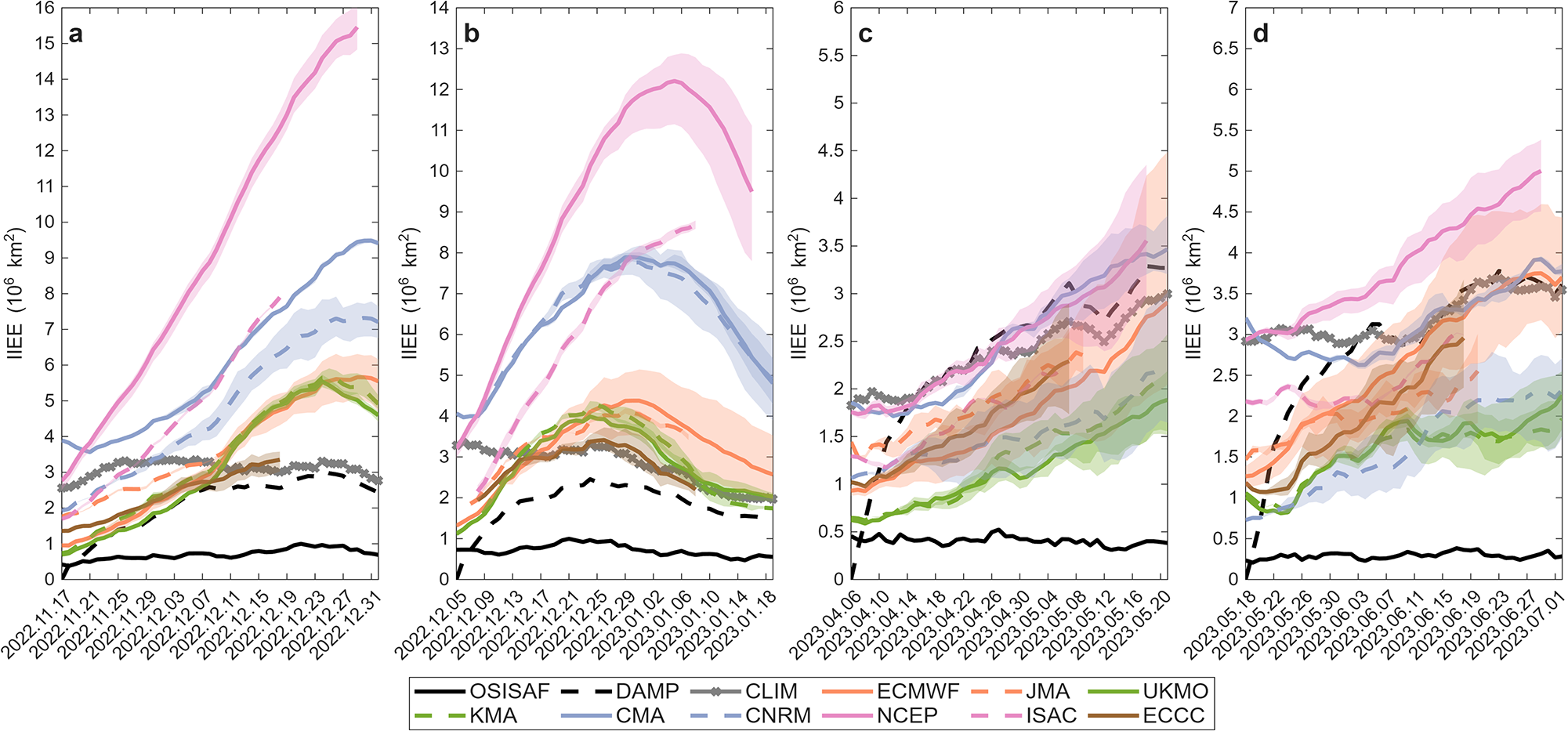
Figure 9 shows a comprehensive evaluation of the IIEE from the S2S models alongside two benchmark methods during four periods. The IIEE between OSISAF and NSIDC remains consistently below 1 × 10⁶ km2 in all periods, indicating that the uncertainty arising solely from the choice of observational SIC dataset is substantially smaller than the forecast errors of most S2S systems. This reference level, therefore, offers a useful context for interpreting the magnitude of model forecast errors relative to initialization uncertainty.
IIEE relative to NSIDC for DAMP, CLIM and S2S models over the four periods. Colored lines denote S2S models, the black dashed line is DAMP of NSIDC, the gray crossed solid line is CLIM of NSIDC and the black solid line denotes the IIEE of OSISAF relative to NSIDC.

For P1, the S2S models display different IIEE on the initial day, ranging from 0.73 to 3.89 × 10⁶ km2 (Fig. 9a). CMA and NCEP have larger IIEE than CLIM, primarily due to the evident overestimation at the outer edge of sea-ice regions. The IIEE metrics for ECMWF, JMA, UKMO, KMA, CNEM, ISAC and ECCC fall between the DAMP and CLIM, with the lowest IIEE for UKMO and KMA.
For the prediction of P1, all models show larger IIEE than DAMP throughout the period. The DAMP-IIEE gradually approached CLIM-IIEE, and the subsequent spatial error patterns (Fig. S12) show that CLIM consistently overestimates the outer edge of the Amundsen Sea. The IIEE of most models increases for 4 weeks and then decreases. CMA and NCEP display consistently higher IIEE than both CLIM and DAMP throughout the entire forecast period, and most of the IIEE is contributed by OE (Fig. S10). Such overestimation extends to all models, and the area covered by overestimation expands as the forecast time increases. This is a direct result of the models predicting a slower rate of sea-ice decline compared to observations (Fig. 1), which likely points to a systematic underestimation of sea-ice melt in the forecasts. This melt bias could potentially be linked to errors in the simulated surface energy budget associated with surface radiative fluxes. It is worth noting that due to a much delayed rapid decrease of SIE (except ISAC and NCEP) in the S2S models mentioned above, the UE gradually increases, primarily occurring in the Weddell Sea, Ross Sea and Indian Ocean sectors.
For P2, the S2S models exhibit a wide range of initial IIEE, ranging from 1.13 to 4.06 × 10⁶ km2 (Fig. 9b). CMA, CNRM and NCEP have larger IIEE than CLIM, primarily due to the evident overestimation along the outer sea-ice margins. In contrast, other models display intermediate IIEE between DAMP and CLIM, with the lowest IIEE for UKMO and KMA.
During the forecast period of P2, all models have larger IIEE than DAMP throughout the entire period. The DAMP-IIEE gradually approached CLIM-IIEE, and the subsequent spatial error patterns are similar to those in P1, with CLIM largely overestimating the sea-ice edge while the UE of DAMP gradually exceeds that of CLIM. The IIEE of most models first increases for 3 weeks and then decreases. Half of the S2S models (e.g. CMA, CNRM and NCEP) display consistently higher IIEE than both CLIM and DAMP throughout the entire forecast period, and most of the IIEE is contributed by OE (Fig. S13). Similar to P1, this overestimation becomes more pronounced over time. Except for ISAC and NCEP, the underestimated ice edge error of other models continues to increase.
At the beginning of P3, the S2S models also display different IIEE, ranging from 0.58 to 1.84 × 10⁶ km2 (Fig. 9c). All models lie between CLIM and DAMP. However, certain models (e.g. JMA, CNRM and CMA) initially have significantly larger UEs than CLIM. The initial spatial error distributions in Fig. S6 reveal that underestimation of CMA occurs along the Antarctic inner ice edge, while JMA and CNRM exhibit notable missed forecasts in the Ross Sea and Indian Ocean sectors, NCEP and ISAC have evident overestimation at all the outer edges.
The forecast results of P3 show that the ice edge errors of all models are larger than those of DAMP during the first 4 days. The DAMP-IIEE gradually approaches and surpasses CLIM-IIEE, which is mainly due to the gradual increase in the underestimation error of DAMP in the Weddell Sea region (Fig. S18). The IIEE of all models increases with forecast days, which also corresponds to the general overestimation of SIE. Among them, CMA and NCEP have comparable IIEE with CLIM and DAMP throughout the forecast period (Fig. 9c). The OE of most S2S models continues to increase slowly (Fig. S16), mainly in the Weddell Sea, the Bellingshausen Sea and the Ross Sea. The UE of UKMO and KMA increases more subsequently, with a missed forecast of SIC in the Amundsen Sea, Ross Sea and Indian Ocean. In addition, JMA, CMA and CNRM keep about 0.7–1.5 × 10⁶ km2 of UE, with the UEs in the regions mentioned above.
On the initial day of P4, the S2S models have larger IIEE than those of P3, ranging from 0.72 to 3.2 × 10⁶ km2 (Fig. 9d). The IIEE of CMA and NCEP is higher than CLIM, mainly driven by the relatively larger OE, which is linked to the overestimation of SIC in the Weddell Sea, Amundsen and Bellingshausen Sea and the Ross Sea. The IIEE of other models falls between DAMP and CLIM, with the lowest IIEE of CNRM.
During P4, the IIEE of all models is larger than DAMP during the first 4 days. The IIEE of DAMP gradually approaches and almost coincides with CLIM, which is mainly due to the gradual increase in the underestimation error of DAMP in the eastern Weddell Sea, similar to P3. The IIEE of all models increases with the forecast length, aligning with the general overestimation of SIE, and the IIEE of NCEP is larger than that of CLIM and DAMP (Fig. 9d). The OE of most S2S models increases more quickly than P3 (Fig. S19), mainly due to overestimation of the SIC at the outer margins of the Weddell Sea, the Bellingshausen Sea and the Ross Sea. The UE of UKMO and KMA subsequently increases more significantly, resulting from the underestimation of SIC in the Amundsen Sea, the Ross Sea and the Indian Ocean.
Overall, the evolution of IIEE across the four prediction periods reveals that S2S models have persistent sea-ice edge errors. Especially in P1 and P2, CMA and NCEP remain significantly higher IIEE than the two benchmarks. Although UKMO and KMA perform comparably to or better than CLIM in P3 and P3, their increasing IIEE indicates underestimation of SIC in key regions such as the Weddell, Ross and Bellingshausen Seas, leading to a systematic shift in marginal ice zones. Importantly, the results suggest that overestimation of marginal sea ice during the growth season is a systematic issue. Furthermore, the sea-ice edge prediction of S2S models shows minimal sensitivity to the choice of reference SIC dataset.
4. Discussion and conclusion
In this paper, we first assess the capability of current operational S2S forecast systems to predict the extremely anomalous Antarctic SIE during the four key periods that lead to the record low seasonal minimum and maximum of Antarctic SIE in 2023. For P1 and P2, we find that all models fail to capture the exceptionally rapid reduction of Antarctic sea ice, though the predictive skill of ECMWF and JMA can approach the CLIM prediction that still shows large differences relative to the verifying sea-ice analysis. Compared to P1, for P2, there are more models (ECMWF, JMA and ECCC) showing predictive skill close to two benchmarks. Some models (UKMO, KMA, CMA, CNRM and ECCC) exhibit the erroneous delayed rapid decrease of SIE during P1 and P2. But for P3 and P4, all S2S models exhibit an overall tendency to overestimate SIE. Two models (UKMO and KMA) are skillful to simulate the anomalously slow recovery, though they have slower growth at the outset during P3 and P4.
Zampieri and others (Reference Zampieri, Goessling and Jung2019) assessed the ability of some S2S forecast systems to predict the location of the sea-ice edge in the Antarctic during 1999–2011. They found that most S2S models overestimate the sea-ice edge extent, and only ECMWF performs better than the two benchmark methods for some lead times. To further assess the Antarctic sea-ice edge prediction of S2S models, we calculate the ice edge errors (including IIEE, OE and UE; Goessling and others, Reference Goessling, Tietsche, Day, Hawkins and Jung2016). It is noteworthy that all S2S models exhibit larger IIEE than DAMP during P1 and P2. For P3 and P4, S2S models have worse sea-ice edge prediction than DAMP in the initial 1 week forecast length; subsequently, some models (ECMWF, JMA, UKMO, KMA and ECCC) outperform DAMP in sea-ice edge prediction. Even UKMO and KMA, which outperform other models in SIE prediction, display the growing UEs over time. These results underscore that even when SIE prediction appears skillful, spatial misrepresentation of the ice edge remains a significant challenge. Overall, while S2S models perform better at predicting the sea-ice edge than the total extent in some cases, systematic errors persist throughout all periods, especially overestimation along the marginal zones.
While our analysis suggests that initial sea-ice state errors play an important role in the low skill in predicting the 2022–23 Antarctic sea ice, we recognize that such low skill may partly reflect uncertainties induced by initialization methods that assimilate the verifying sea-ice data to generate initialization, which is particularly important for shorter forecast lengths (≤7 days). Then, the subsequent biases are contributed to by model drift. First, substantial initial SIE biases, as shown by the strong correlation between initial and cumulative SIE errors, highlight deficiencies in sea-ice initialization. Second, after initialization, most S2S models quickly diverge from the verifying sea-ice analysis, as forecasts tend to revert toward the model’s climatology regardless of initial accuracy (Magnusson and others, Reference Magnusson, Alonso-Balmaseda, Corti, Molteni and Stockdale2013; Fučkar and others, Reference Fučkar, Volpi, Guemas and Doblas-Reyes2014), which can be found in the forecasts of the S2S models starting from different initial times (Figs S22 and S23). This drift amplifies initial errors, particularly during the rapid decline phase, and it appears that some models, including ECMWF, UKMO, KMA and JMA, show some capability to pick up the tendency of the observed rapid decline, as the initial sea-ice condition has gradually carried more signal of rapid melting of Antarctic sea ice resulting from synoptic-scale circulation patterns (Xiu and others, Reference Xiu, Luo, Yang, Tietsche, Day and Chen2022). The subsequent evolution of UKMO and KMA still depends on the model itself and, therefore, deviates from the verifying sea-ice analysis. However, some models still exhibit erroneous SIE evolution and very large biases. For P3, model drift still exists but is generally weaker, and most models (except CNRM, NCEP and ISAC) gradually reduce the errors with delayed initial times. Thus, with more sea-ice anomaly information assimilated, the initial sea-ice state might be more realistic and skillful (Yang and others, Reference Yang, Losa, Losch, Jung and Nerger2015).
Our additional analyses confirm that SST biases, especially negative biases north of the ice edge during the advancing phase in P3 and P4 (Figs S7 and S9), contribute to the overestimation of SIE by most S2S models. A significant negative correlation between SST bias and cumulative SIE bias highlights the importance of accurate SST initialization. These results underscore the key role of ocean data assimilation in improving Antarctic sea-ice forecasts, in line with recent findings (Purich and Doddridge, Reference Purich and Doddridge2023; Espinosa and others, Reference Espinosa, Blanchard-Wrigglesworth and Bitz2024).
Our analyses suggest that the low skill in predicting exceptionally low Antarctic sea ice during 2022–23 also comes from inadequate ability to simulate the strength and pattern of synoptic atmospheric circulation and sea-ice evolution (Blanchard-Wrigglesworth and others, Reference Blanchard-Wrigglesworth, Roach, Donohoe and Ding2021). The regional SLP gradient bias is positively correlated with the accumulated SIE bias to a certain extent. It seems that the models employing more advanced representations of sea-ice processes (i.e. CICE5.1.2 and LIM2) tend to show relatively better predictive skill. It is worth further investigation whether such a sea-ice model better reflects interactions between the atmosphere and sea ice and the evolution of sea ice. Furthermore, the progression of the melt season and the eventual determination of the minimum ice extent also rely significantly on the influence of local atmospheric extremes occurring on a synoptic timescale (Turner and others, Reference Turner2022), and the internal variability also accounts for the discrepancy between verifying analysis and prediction (Screen and others, Reference Screen, Deser, Simmonds and Tomas2014; Zhang and others, Reference Zhang2022). Thus, S2S forecast systems that have difficulty capturing such extremes well cannot predict the extremely anomalous sea-ice changes.
Given that both the initial sea-ice conditions, the initial ocean conditions and the predicted atmospheric circulations have crucial effects on the prediction of extreme Antarctic sea-ice change, further research will be conducted to understand which factor leads to larger prediction errors. Additionally, it is worth noting that the predictive skill of S2S systems could be significantly improved through calibration using historical forecasts (hindcasts) (Dirkson and others, Reference Dirkson, Denis, Merryfield, Peterson and Tietsche2022), a practical approach to mitigate inherent model climatological biases identified in this study. Future work will also explore bias-corrected forecasts to further assess the potential of S2S systems in predicting extreme Antarctic sea-ice anomalies.
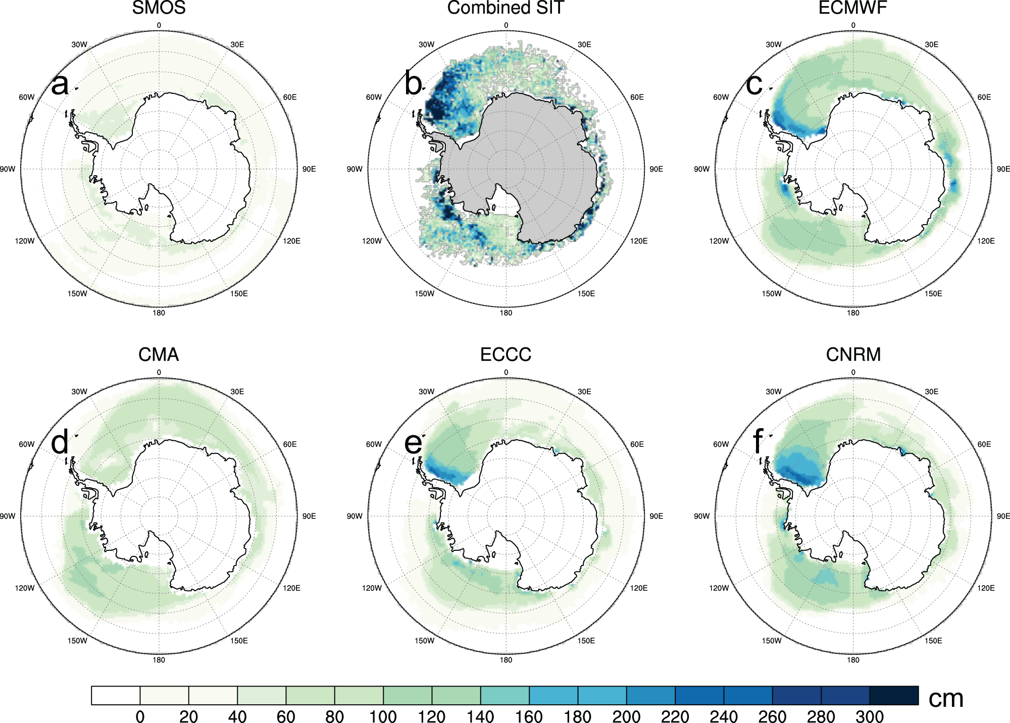
Previous studies have demonstrated the importance of SIT initialization for improving SIE prediction, both in idealized perfect-model experiments (Day and others, Reference Day, Hawkins and Tietsche2014; Ordoñez and others, Reference Ordoñez, Bitz and Blanchard-Wrigglesworth2018) and in operational forecasting systems through assimilation of observed thickness (Blockley and Peterson, Reference Blockley and Peterson2018). As shown in Fig. 10, the SIT simulated by the S2S models deviates substantially from the verifying sea-ice analysis in November. However, we note that existing Antarctic SIT products have important limitations in both thickness range and temporal applicability and cannot be regarded as a definitive reference for the 2022–23 period. Therefore, while these differences suggest a potential role of initial SIT biases in subsequent SIE forecast errors, a quantitative verification against observations is not possible at present.
(a) Spatial distribution of the monthly mean SIT in November 2022 from the SMOS dataset. (b) Spatial distribution of the monthly mean SIT in November 2022 from the combined observed SIT. (c–f) Spatial distribution of the averaged SIT of S2S models from 17 November 2022 to 31 November 2022 during P1.

Supplementary material
The supplementary material for this article can be found at https://doi.org/10.1017/jog.2026.10162.
Data availability statement
All data analyzed in this paper are openly available. The S2S real-time database is hosted at CMA and ECMWF, which can be retrieved from the CMA data portal at https://s2s.cma.cn/dmodelsa and the ECMWF data portal at https://apps.ecmwf.int/datasets/data/s2s/levtype=sfc/type=cf/. The satellite-derived Antarctic sea-ice concentration data of NSIDC-0051 can be retrieved from https://nsidc.org/data/nsidc-0051/versions/2, and that of OSI-430-a can be retrieved from https://thredds.met.no/thredds/catalog/osisaf/met.no/reprocessed/ice/conc_cra_files/catalog.Html, and OSI-450-a1 can be retrieved from https://osi-saf.eumetsat.int/products/osi-450-a1#citation_product. The hourly mean sea level pressure (SLP) data can be retrieved from the European Center for Medium-Range Weather Forecasts (ECMWF) at https://cds.climate.copernicus.eu/cdsapp#!/dataset/reanalysis-era5-single-levels?tab=form. The NOAA daily Optimum Interpolation Sea Surface Temperature dataset (OISST) is obtained from https://www.ncei.noaa.gov/data/sea-surface-temperature-optimum interpolation/v2.1/. The sea-ice thickness from SMOS (https://seaice.uni-bremen.de/data-archive/) and the combined observed sea-ice thickness (https://zenodo.org/records/12783561) are used in the discussion.
Acknowledgements
The authors thank two anonymous reviewers for their thorough reviews and constructive comments, helping to improve the manuscript. This research is supported by the National Natural Science Foundation of China (U2542215, 42376237) and the Southern Marine Science and Engineering Guangdong Laboratory (Zhuhai) (SML2024SP023). We also acknowledge the high-performance computing support from the School of Atmospheric Science of Sun Yat-sen University. This work is based on S2S data. S2S is a joint initiative of the World Weather Research Programme (WWRP) and the World Climate Research Programme (WCRP). The original S2S database is hosted at ECMWF as an extension of the TIGGE database.


 Open access

