


1 Introduction
Let X be a smooth projective variety and $D = D_1 + \dots + D_r \subset X$
be a simple normal crossings divisor whose irreducible components are nef. The local/logarithmic correspondence connects two enumerative theories associated to
$D = D_1 + \dots + D_r \subset X$
be a simple normal crossings divisor whose irreducible components are nef. The local/logarithmic correspondence connects two enumerative theories associated to $(X,D)$
: rational curves in X with maximal tangency to D, and rational curves in the total space of
$(X,D)$
: rational curves in X with maximal tangency to D, and rational curves in the total space of $\mathcal {O}_{X}(-D)$
. This correspondence was conjectured by Takahashi [Reference TakahashiTak01] and proved by Gathmann [Reference GathmannGat03], for the Gromov–Witten theory of
$\mathcal {O}_{X}(-D)$
. This correspondence was conjectured by Takahashi [Reference TakahashiTak01] and proved by Gathmann [Reference GathmannGat03], for the Gromov–Witten theory of $X= \mathbb {P}^2$
and D a smooth cubic, and then generalised in [Reference van Garrel, Graber and RuddatvGGR19] to arbitrary X and D any smooth, nef divisor.
$X= \mathbb {P}^2$
and D a smooth cubic, and then generalised in [Reference van Garrel, Graber and RuddatvGGR19] to arbitrary X and D any smooth, nef divisor.
1.1 Results
We prove a quasimap local/logarithmic correspondence, for simple normal crossings divisors, under a mild positivity assumption. Let $X = W /\!\!/ G$
be a GIT quotient and let
$X = W /\!\!/ G$
be a GIT quotient and let $D = D_1 + \dots + D_r \subset X$
be a simple normal crossings divisor satisfying Assumptions 2.1 and 3.1.
$D = D_1 + \dots + D_r \subset X$
be a simple normal crossings divisor satisfying Assumptions 2.1 and 3.1.
This includes toric varieties and partial flag varieties, with any simple normal crossings divisor, as well as complete intersections in these spaces with divisors pulled back from the ambient space. There are two different directions in which to generalise the local/logarithmic correspondence for smooth divisors. When tangency is imposed with respect to all divisor components simultaneously we prove a local/logarithmic correspondence for arbitrary r.
Theorem A (Theorem 5.20).
Suppose $D_1 \cap \dots \cap D_r \neq \emptyset $
and the components of D are very ample. Then we have the following equality of virtual classes
$D_1 \cap \dots \cap D_r \neq \emptyset $
and the components of D are very ample. Then we have the following equality of virtual classes
 $$ \begin{align*} [\mathcal{Q}_{0,(\underline{d},0)}^{\log}(X|D,\beta)]^{\mathrm{vir}} = \prod_{i=1}^r(-1)^{d_i+1} \cdot \operatorname{\mathrm{ev}}_1^* D_i \cap [\mathcal{Q}_{0,2}(\oplus_{i=1}^r\mathcal{O}_{X}(-D_i),\beta)]^{\mathrm{vir}}, \end{align*} $$
where on the left-hand side maximal tangency is imposed to $D_1 \cap \dots \cap D_r$
at a single point.
$D_1 \cap \dots \cap D_r$
at a single point.
For $r=1$
, in Gromov–Witten theory, this is the strong form of the smooth local/logarithmic correspondence (see [Reference Tseng and YouTY23b, Conjecture 18]). The original form is obtained by using the divisor equation and is the main theorem of [Reference van Garrel, Graber and RuddatvGGR19]. The authors of [Reference van Garrel, Graber and RuddatvGGR19] conjectured a different generalisation for D an s.n.c. divisor, where maximal tangency is imposed to the components of the divisor at distinct points. Figure 4 exhibits the difference between the generalisations. Although there is some numerical evidence for either generalisation [Reference Bousseau, Brini and van GarrelBBvG24, Reference Bousseau, Brini and van GarrelBBvG22], the authors of [Reference Nabijou and RanganathanNR22] showed that even if
$r=1$
, in Gromov–Witten theory, this is the strong form of the smooth local/logarithmic correspondence (see [Reference Tseng and YouTY23b, Conjecture 18]). The original form is obtained by using the divisor equation and is the main theorem of [Reference van Garrel, Graber and RuddatvGGR19]. The authors of [Reference van Garrel, Graber and RuddatvGGR19] conjectured a different generalisation for D an s.n.c. divisor, where maximal tangency is imposed to the components of the divisor at distinct points. Figure 4 exhibits the difference between the generalisations. Although there is some numerical evidence for either generalisation [Reference Bousseau, Brini and van GarrelBBvG24, Reference Bousseau, Brini and van GarrelBBvG22], the authors of [Reference Nabijou and RanganathanNR22] showed that even if $D = D_1 + D_2$
, both generalisations can fail in Gromov–Witten theory. In addition to Theorem A, we show that the strong form version of the conjecture of [Reference van Garrel, Graber and RuddatvGGR19] is true for quasimaps for
$D = D_1 + D_2$
, both generalisations can fail in Gromov–Witten theory. In addition to Theorem A, we show that the strong form version of the conjecture of [Reference van Garrel, Graber and RuddatvGGR19] is true for quasimaps for $r=2$
.
$r=2$
.
Theorem B (Theorem 5.19).
Suppose that $D=D_1 + D_2$
has two components, which are very ample. Then we have the following equality of virtual classes
$D=D_1 + D_2$
has two components, which are very ample. Then we have the following equality of virtual classes
 $$ \begin{align*}[\mathcal{Q}_{0,(d_1,d_2)}^{\log}(X|D_1 + D_2,\beta)]^{\mathrm{vir}} = (-1)^{d_1+d_2} \cdot \prod_{i=1}^2 \operatorname{\mathrm{ev}}_i^*D_i \cap [\mathcal{Q}_{0,2}(\oplus_{i=1}^2\mathcal{O}_{X}(-D_i),\beta)]^{\mathrm{vir}}.\end{align*} $$
In fact, [Reference Tseng and YouTY23b, Conjecture 18] gives a much more general local/logarithmic conjecture for simple normal crossings divisors. The situations in Theorems A and B are the two extremes.
In order to prove Theorem A (as well as Theorem B), we reduce to the case where $r=1$
in Theorems 5.21 and 5.26 by showing that, for products of projective spaces relative toric boundary divisors, the simple normal crossings logarithmic quasimap spaces can be obtained as fibre products of logarithmic quasimap spaces for smooth divisors. Then, following the strategy of [Reference van Garrel, Graber and RuddatvGGR19], we prove Theorem A in the case where
$r=1$
in Theorems 5.21 and 5.26 by showing that, for products of projective spaces relative toric boundary divisors, the simple normal crossings logarithmic quasimap spaces can be obtained as fibre products of logarithmic quasimap spaces for smooth divisors. Then, following the strategy of [Reference van Garrel, Graber and RuddatvGGR19], we prove Theorem A in the case where $r=1$
using a degeneration formula for quasimaps which we develop.
$r=1$
using a degeneration formula for quasimaps which we develop.
Let $W \rightarrow \mathbb {A}^1$
be a toric double point degeneration. An example is the deformation to the normal cone of a smooth projective toric variety along a smooth toric divisor. Let
$W \rightarrow \mathbb {A}^1$
be a toric double point degeneration. An example is the deformation to the normal cone of a smooth projective toric variety along a smooth toric divisor. Let $X_0$
denote the central fibre, which is a union of two toric varieties
$X_0$
denote the central fibre, which is a union of two toric varieties $X_1$
and
$X_1$
and $X_2$
glued along a common toric divisor D.
$X_2$
glued along a common toric divisor D.
Theorem C (Degeneration formula for quasimaps, Theorem 4.20).
 $$ \begin{align*} [\mathcal{Q}_{g,n}^{\log}(X_0,\beta)]^{\mathrm{vir}} = \sum_{\widetilde{\Gamma}} \frac{m_{\widetilde{\Gamma}}}{|\mathrm{Aut}(\widetilde{\Gamma})|} j_{\widetilde{\Gamma},*} c_{\widetilde{\Gamma}}^* \, \Delta^! \left(\prod_{V \in V(\widetilde{\Gamma})} [\mathcal{Q}^{\log}_{g_V,\alpha_V}(X_{r(V)}|D,\beta_V)]^{\mathrm{vir}}\right) \end{align*} $$
Both the proof and application of the degeneration formula for quasimaps entail additional subtleties, when compared with stable maps. The main one is based on the fact that quasimap spaces do not embed along closed embeddings, see [Reference Battistella and NabijouBN21, Remark 2.3.3]. As a consequence, if V is a toric subvariety of a toric variety X, then quasimaps to X which factor through V contain more information than quasimaps to V with its toric presentation, as we illustrate in Example 2.9. We show in Example 2.8 that this phenomenon is relevant when studying toric double point degenerations, and it forces us to consider non-toric presentations for the irreducible components of the special fibre. As a result, the output of the degeneration formula, Theorem 4.20, may contain curve classes which live on the degeneration family, rather than on the irreducible components of the special fibre. We call such curve classes ghost classes (see Definition 2.10). For the application to the local/logarithmic correspondence, these contributions are ruled out in Proposition 5.17. To prove Proposition 5.17 we show that these contributions have a trivial excess line bundle.
1.2 Motivation
Relative or logarithmic Gromov–Witten theory [Reference ChenChe14b, Reference Gross and SiebertGS13, Reference Abramovich and ChenAC14, Reference LiLi01] has significantly shaped the landscape of enumerative geometry. The resulting invariants (and their generalisations) have proved important in mirror symmetry constructions [Reference Gross and SiebertGS22], degeneration formulas [Reference RanganathanRan22, Reference GrossGro23, Reference Kim, Lho and RuddatKLR21, Reference LiLi02, Reference Abramovich, Chen, Gross and SiebertACGS21], tropical correspondence theorems such as [Reference Mandel and RuddatMR20, Reference GrossGro18, Reference GraefnitzGra22, Reference Nishinou and SiebertNS06] as well as understanding the tautological ring of the moduli space of curves [Reference Graber and VakilGV05, Reference Ranganathan and Urundolil KumaranRK23, Reference Molcho and RanganathanMR23, Reference Holmes, Molcho, Pandharipande, Pixton and SchmittHMP+22]. Consequently, computing logarithmic Gromov–Witten invariants is an important problem in enumerative algebraic geometry.
An interesting feature of the local/logarithmic correspondence is that the two sides can be understood by qualitatively different techniques, especially when the logarithmic divisor is genuinely simple normal crossings. Thus, conceptually moving to one side and then using its features can be profitable. Although there have been many numerical generalisations and variations of this correspondence [Reference Bousseau, Fan, Guo and WuBFGW21, Reference van Garrel, Nabijou and SchulervGNS24, Reference Bousseau, Brini and van GarrelBBvG21, Reference Bousseau, Brini and van GarrelBBvG24, Reference Bousseau, Brini and van GarrelBBvG22], the original cycle level correspondence holds in the case where the divisor is smooth. On the other hand, the major difficulty in computing logarithmic Gromov–Witten invariants, at least in genus zero, lies in the case where the divisor is genuinely simple normal crossings.
1.3 The role of quasimaps
There have been conjectures to generalise the local/logarithmic correspondence to the case where the divisor is simple normal crossings, but as we have remarked these conjectures are false in general, in Gromov–Witten theory [Reference Nabijou and RanganathanNR22]. Moreover, the authors noticed [Reference Nabijou and RanganathanNR22, Remark 5.4] that one point of view for the underlying reason for the failure of these conjectures was the presence of excess components in the moduli space containing rational tails. Quasimap theory [Reference Marian, Oprea and PandharipandeMOP11, Reference Ciocan-Fontanine and KimCFK10, Reference Ciocan-Fontanine, Kim and MaulikCFKM14] provides an alternative framework for counting curves which excludes rational tails, and so it is conceivable that these are no longer counterexamples in the quasimap setting.
The origins of quasimap theory are intertwined with its connections to mirror symmetry [Reference Ciocan-Fontanine and KimCFK14] and the main applications of the theory have been wall-crossing formulas which relate Gromov–Witten invariants to quasimap invariants [Reference Ciocan-Fontanine and KimCFK14, Reference Ciocan-Fontanine and KimCFK17, Reference ZhouZho22]. These wall-crossing formulas reduce computations in Gromov–Witten theory to quasimap theory, which are typically easier. Indeed, almost all results that allow us to compute genus-zero Gromov–Witten invariants [Reference GiventalGiv98] rely at heart on the wall-crossing formula. Recently, the third author has developed a theory of logarithmic quasimaps [Reference ShafiSha24] with the expectation of proving logarithmic wall-crossing formulas, first proposed in [Reference Battistella and NabijouBN21]. A consequence of Theorem A and Theorem B, which confirm the predictions of [Reference Nabijou and RanganathanNR22], is that the techniques of ordinary Gromov–Witten/quasimap theory can be imported over to compute logarithmic quasimap invariants in the case where the divisor is genuinely simple normal crossings. Combining this with a conjectural wall-crossing should be a powerful method for computing logarithmic Gromov–Witten invariants.
1.4 Quasimaps and the degeneration formula
The degeneration formula for double point degenerations [Reference LiLi02, Reference ChenChe14a, Reference Kim, Lho and RuddatKLR21, Reference Abramovich and FantechiAF16] has been a well-used tool in Gromov–Witten theory since its first introduction to the subject [Reference Maulik and PandharipandeMP06, Reference Okounkov and PandharipandeOP09, Reference Pandharipande and PixtonPP17]. For all the same reasons the degeneration formula for quasimaps, Theorem C, will provide similar computational capabilities. In this paper we use the degeneration formula to prove the local/logarithmic correspondence for smooth pairs. There is a related direction to this, which is the prospect of investigating holomorphic anomaly equations in the relative setting, for which quasimaps are better suited.
In the absolute setting, for Calabi–Yau threefolds, the wall-crossing formula coincides with the mirror map and hence quasimap invariants are exactly equal to the B-model invariants of the mirror. This link has been exploited to give a direct geometric proof, for local $\mathbb {P}^2$
, of the holomorphic anomaly equation [Reference Lho and PandharipandeLP18], which gives profound structure to the Gromov–Witten theory of a Calabi–Yau, coming from the B-model. Using the double point degeneration formula, the authors of [Reference Bousseau, Fan, Guo and WuBFGW21] prove a holomorphic anomaly equation for the logarithmic Gromov–Witten theory of
$\mathbb {P}^2$
, of the holomorphic anomaly equation [Reference Lho and PandharipandeLP18], which gives profound structure to the Gromov–Witten theory of a Calabi–Yau, coming from the B-model. Using the double point degeneration formula, the authors of [Reference Bousseau, Fan, Guo and WuBFGW21] prove a holomorphic anomaly equation for the logarithmic Gromov–Witten theory of $\mathbb {P}^2$
relative an elliptic curve. This suggests that more general holomorphic anomaly equations in relative geometries could be pursued using the degeneration formula for quasimaps, after generalising this beyond the toric setting.
$\mathbb {P}^2$
relative an elliptic curve. This suggests that more general holomorphic anomaly equations in relative geometries could be pursued using the degeneration formula for quasimaps, after generalising this beyond the toric setting.
1.5 Future directions
1.5.1 Local/logarithmic correspondence in higher genus
There are two ways in which one can generalise the original smooth local/logarithmic correspondence. Either to increase the rank of the divisor, as we have addressed in the present paper, or to generalise from rational curves to higher genus curves, where on the logarithmic side one adds a $\lambda _g$
class for the dimensions to match. In Gromov–Witten theory both generalisations fail on the nose, for the higher genus situation there are correction terms described in [Reference Bousseau, Fan, Guo and WuBFGW21]. One can speculate about whether, analogous to the situation for higher rank divisors, there are instances where the correction terms vanish for the quasimap local/logarithmic correspondence in higher genus.
$\lambda _g$
class for the dimensions to match. In Gromov–Witten theory both generalisations fail on the nose, for the higher genus situation there are correction terms described in [Reference Bousseau, Fan, Guo and WuBFGW21]. One can speculate about whether, analogous to the situation for higher rank divisors, there are instances where the correction terms vanish for the quasimap local/logarithmic correspondence in higher genus.
1.5.2 Holomorphic anomaly equations
In the Gromov–Witten situation, the relationship between local and logarithmic invariants in higher genus is used to prove a holomorphic anomaly equation for $\mathbb {P}^2$
relative to an elliptic curve. Since quasimaps are better suited to understanding holomorphic anomaly equations, a natural is to pursue this for other geometries.
$\mathbb {P}^2$
relative to an elliptic curve. Since quasimaps are better suited to understanding holomorphic anomaly equations, a natural is to pursue this for other geometries.
In order to accomplish this, the degeneration formula would need to be generalised beyond the toric setting. This should be possible however. The main difficulty in quasimap theory is the restriction of the theory to spaces admitting a certain GIT presentation. Even the deformation to the normal cone of a toric variety along a smooth, non-toric divisor is no longer toric. On the other hand, one can rewrite the total space, as well as more general blow-ups, as a GIT quotient, see, for example, [Reference Coates, Lutz and ShafiCLS22, Proposition 6.2].
1.5.3 Orbifold/logarithmic correspondence
The local/logarithmic correspondence concerns invariants with maximal contact to the divisor which makes it fertile testing ground, but many of the ideas pursued here should extend to a more general context. An alternative approach to tangency involves replacing components of divisor with roots [Reference CadmanCad07], and using the framework of orbifold Gromov–Witten theory to produce invariants [Reference Tseng and YouTY23a]. There has been effort to compare the logarithmic theories with the resulting orbifold theory [Reference Abramovich, Cadman and WiseACW17, Reference Battistella, Nabijou and RanganathanBNR23, Reference Tseng and YouTY20], since the latter is significantly easier to compute in practice. However, it computes a different set of invariants in general, which do not immediately interact with degeneration formulas and lacks some of the conceptual advantages of the logarithmic theory. Furthermore, no known structure organises the difference between the theories.
Our work here sheds some light on this difference. One can view the local theory defined by an s.n.c. divisor as a sector of this orbifold by the results of [Reference Battistella, Nabijou, Tseng and YouBNTY23], and so our results suggest that the difference between the computable orbifold theory and the conceptually better logarithmic theory, might be controlled in part by mirror maps. There is a related proposal in [Reference YouYou22].
Taking these issues together, it seems reasonable that orbifold and logarithmic Gromov–Witten theory for pairs should be compared via the quasimap theory, where at least in some sectors such as the one we study here, the invariants coincide. The general picture appears to be more complicated, but the significantly simplified combinatorics of quasimaps provides a clear path to computations.
2 Absolute quasimaps
Here we recall the definition of absolute GIT quasimaps from [Reference Ciocan-Fontanine, Kim and MaulikCFKM14].
Assumption 2.1. Let $Z= \operatorname {Spec} A$
be an affine algebraic variety with an action by a reductive algebraic group G. Let
$Z= \operatorname {Spec} A$
be an affine algebraic variety with an action by a reductive algebraic group G. Let $\theta $
be a character inducing a linearisation for the action. We insist that
$\theta $
be a character inducing a linearisation for the action. We insist that
-
• $Z^s = Z^{ss}$
-
•
$Z^s$
is nonsingular -
• G acts freely on
$Z^s$
-
• Z has only l.c.i. singularities


Then quasimaps to $Z /\!\!/ G$
are defined as follows.
$Z /\!\!/ G$
are defined as follows.
Definition 2.2. Fix non-negative integers $g,n$
and
$g,n$
and $\beta \in \operatorname {\mathrm {Hom}}(\operatorname {\mathrm {Pic}}^G Z, \mathbb {Z})$
. An n-marked stable quasimap of genus g and degree
$\beta \in \operatorname {\mathrm {Hom}}(\operatorname {\mathrm {Pic}}^G Z, \mathbb {Z})$
. An n-marked stable quasimap of genus g and degree $\beta $
to
$\beta $
to $Z /\!\!/ G$
is
$Z /\!\!/ G$
is
 $$ \begin{align*} \left((C, p_1, \dots, p_n), u \right) \end{align*} $$
where
-
(1)
$(C, p_1, \dots , p_n)$
is an n-marked prestable curve of genus g. -
(2)
$u: C \rightarrow [Z/G]$
of class
$\beta $
(i.e.
$\beta (L) = \deg _C u^*L$
).


which satisfy
-
(1) (Non-degeneracy) there is a finite (possibly empty) set
$B \subset C$
, distinct from the nodes and markings, such that
$\forall c \in C \setminus B$
we have
$u(c) \in Z^s$
. -
(2) (Stability)
$\omega _C(p_1 + \cdots + p_n) \otimes L_{\theta }^{\epsilon }$
is ample
$\forall \epsilon \in \mathbb {Q}_{>0}$
, where
$L_{\theta }$
comes from the linearisation.


Theorem 2.3 [Reference Ciocan-Fontanine, Kim and MaulikCFKM14].
Let $X = Z /\!\!/ G$
with Z and G as in Assumption 2.1. The moduli stack of stable quasimaps
$X = Z /\!\!/ G$
with Z and G as in Assumption 2.1. The moduli stack of stable quasimaps $\mathcal {Q}_{g,n}(X,\beta )$
is a Deligne–Mumford stack. If X is proper then so is
$\mathcal {Q}_{g,n}(X,\beta )$
is a Deligne–Mumford stack. If X is proper then so is $\mathcal {Q}_{g,n}(X,\beta )$
. Moreover, it admits a perfect obstruction over
$\mathcal {Q}_{g,n}(X,\beta )$
. Moreover, it admits a perfect obstruction over $\mathfrak {M}_{g,n}$
leading to a virtual fundamental class
$\mathfrak {M}_{g,n}$
leading to a virtual fundamental class $[\mathcal {Q}_{g,n}(X,\beta )]^{\mathrm {vir}}$
.
$[\mathcal {Q}_{g,n}(X,\beta )]^{\mathrm {vir}}$
.
In an earlier iteration of the theory in [Reference Ciocan-Fontanine and KimCFK10], toric quasimaps are defined for toric varieties using the description of the functor of points of a smooth toric variety in terms of line bundle-section pairs according to rays of the fan, proved in [Reference CoxCox95]. In the general context of Definition 2.2, toric quasimaps are recovered by taking the standard GIT presentation coming from toric geometry.
We will prove a degeneration formula in a toric context, which means the double point degeneration will be a toric morphism. However, we will still require the more general definition of quasimaps, Definition 2.2, even in this context, because the process of gluing a quasimap is more subtle than in the case of maps (see the discussion and examples in Section 2.1). Specifically in order to glue together quasimaps to the components of the central fibre we require the GIT presentation induced by the embedding in the total space, rather than the ordinary toric presentation.
Definition 2.4. A toric double point degeneration $W \rightarrow \mathbb {A}^1$
is a double point degeneration with W a toric variety and
$W \rightarrow \mathbb {A}^1$
is a double point degeneration with W a toric variety and $W \rightarrow \mathbb {A}^1$
a toric morphism. By double point degeneration we mean that
$W \rightarrow \mathbb {A}^1$
a toric morphism. By double point degeneration we mean that $W \rightarrow \mathbb {A}^1$
is a flat, proper morphism, with W smooth. The general fibre is smooth and the fibre over
$W \rightarrow \mathbb {A}^1$
is a flat, proper morphism, with W smooth. The general fibre is smooth and the fibre over $0 \in \mathbb {A}^1$
is a reduced union of two irreducible components glued along a common smooth divisor.
$0 \in \mathbb {A}^1$
is a reduced union of two irreducible components glued along a common smooth divisor.
Notation 2.5. We denote the general fibre of a toric double point degeneration $W\to \mathbb {A}^1$
by X. The central fibre
$W\to \mathbb {A}^1$
by X. The central fibre $X_0$
is a union of the two components
$X_0$
is a union of the two components $X_1$
and
$X_1$
and $X_2$
glued along a common smooth divisor D. Necessarily the fan of W has two distinguished rays which map surjectively to the ray in the fan of
$X_2$
glued along a common smooth divisor D. Necessarily the fan of W has two distinguished rays which map surjectively to the ray in the fan of $\mathbb {A}^1$
. These rays correspond to the divisors
$\mathbb {A}^1$
. These rays correspond to the divisors $X_1$
and
$X_1$
and $X_2$
of W, and will typically be denoted by
$X_2$
of W, and will typically be denoted by $\rho _1$
and
$\rho _1$
and $\rho _2$
. All the other rays are contained in a codimension 1 sublattice, as in Figure 1. We will denote the toric GIT presentation of W by
$\rho _2$
. All the other rays are contained in a codimension 1 sublattice, as in Figure 1. We will denote the toric GIT presentation of W by $\mathbb {A}^M /\!\!/ \mathbb {G}_m^s$
and the ambient stack
$\mathbb {A}^M /\!\!/ \mathbb {G}_m^s$
and the ambient stack $[\mathbb {A}^M/ \mathbb {G}_m^s]$
by
$[\mathbb {A}^M/ \mathbb {G}_m^s]$
by $\mathcal {W}$
.
$\mathcal {W}$
.
A double point degeneration has two special rays $\rho _1,\rho _2$
, which project to the generator of the fan of
$\rho _1,\rho _2$
, which project to the generator of the fan of $\mathbb {A}^1$
inside a line L. All other rays are contained in the hyperplane
$\mathbb {A}^1$
inside a line L. All other rays are contained in the hyperplane $L^\perp $
.
$L^\perp $
.

Remark 2.6. The morphism $W\to \mathbb {A}^1$
extends to
$W\to \mathbb {A}^1$
extends to $\mathcal {W}$
because restriction induces an isomorphism
$\mathcal {W}$
because restriction induces an isomorphism $\operatorname {\mathrm {Pic}}(\mathcal {W})\to \operatorname {\mathrm {Pic}}(W)$
. Indeed the unstable locus in the GIT presentation of W has codimension at least 2 [Reference Cox, Little and SchenckCLS11, Proposition 5.1.6], so W and
$\operatorname {\mathrm {Pic}}(\mathcal {W})\to \operatorname {\mathrm {Pic}}(W)$
. Indeed the unstable locus in the GIT presentation of W has codimension at least 2 [Reference Cox, Little and SchenckCLS11, Proposition 5.1.6], so W and $\mathcal {W}$
are isomorphic in codimension 1.
$\mathcal {W}$
are isomorphic in codimension 1.
Remark 2.7. Just as in Gromov–Witten theory one can consider quasimaps over a base. Since this is not addressed in the literature we just make the observation that for a double point degeneration $W \rightarrow \mathbb {A}^1$
we have that
$W \rightarrow \mathbb {A}^1$
we have that $\mathcal {Q}_{g,n}(W/\mathbb {A}^1,\beta ) = \mathcal {Q}_{g,n}(W,\beta )$
, because any quasimap to W necessarily lives in a fibre over
$\mathcal {Q}_{g,n}(W/\mathbb {A}^1,\beta ) = \mathcal {Q}_{g,n}(W,\beta )$
, because any quasimap to W necessarily lives in a fibre over $\mathbb {A}^1$
.
$\mathbb {A}^1$
.
2.1 Quasimaps to a double point degeneration
The degeneration formula involves the study of quasimaps to a double point degeneration $W\to \mathbb {A}^1$
, which we assume to be toric. Let
$W\to \mathbb {A}^1$
, which we assume to be toric. Let $\mathbb {A}^M /\!\!/ \mathbb {G}_m^s$
be the toric GIT presentation of W. We define quasimaps to
$\mathbb {A}^M /\!\!/ \mathbb {G}_m^s$
be the toric GIT presentation of W. We define quasimaps to $X_0$
via the following Cartesian diagram.
$X_0$
via the following Cartesian diagram.

The degeneration formula will express the virtual class of $[\mathcal {Q}_{g,n}(X_0,\beta )]^{\mathrm {vir}}$
, defined via Gysin pullback in the above diagram, with the virtual classes of logarithmic quasimap spaces of
$[\mathcal {Q}_{g,n}(X_0,\beta )]^{\mathrm {vir}}$
, defined via Gysin pullback in the above diagram, with the virtual classes of logarithmic quasimap spaces of $X_1$
and
$X_1$
and $X_2$
relative to D. For stable maps, one has that a map to
$X_2$
relative to D. For stable maps, one has that a map to $X_0$
is the same as a collection of maps to
$X_0$
is the same as a collection of maps to $X_i$
gluing at the nodes. The analogue statement for quasimaps is true only if we take the GIT presentation
$X_i$
gluing at the nodes. The analogue statement for quasimaps is true only if we take the GIT presentation $X_i \simeq \mathbb {A}^{M-1}/\!\!/ \mathbb {G}_m^s$
induced by W, which in general does not agree with the standard toric presentation. Example 2.8 provides a concrete example of this phenomenon.
$X_i \simeq \mathbb {A}^{M-1}/\!\!/ \mathbb {G}_m^s$
induced by W, which in general does not agree with the standard toric presentation. Example 2.8 provides a concrete example of this phenomenon.
Example 2.8. Consider the deformation to the normal cone of $\mathbb {P}^1$
relative
$\mathbb {P}^1$
relative $\infty $
,
$\infty $
, $W=\operatorname {\mathrm {Bl}}_{\infty \times 0}(\mathbb {P}^1\times \mathbb {A}^1)$
. The fan of W, pictured in Figure 2, induces the following GIT presentation
$W=\operatorname {\mathrm {Bl}}_{\infty \times 0}(\mathbb {P}^1\times \mathbb {A}^1)$
. The fan of W, pictured in Figure 2, induces the following GIT presentation
 $$\begin{align*}W = \mathbb{A}^4/\!\!/ \mathbb{G}_m^2, \, \, \mathrm{where} \, \, (\lambda,\mu)\cdot (x_0,x_1,v_1,v_2) = (\lambda\mu x_0,\lambda x_1,\mu v_1, \mu^{-1}v_2). \end{align*}$$
Setting $v_1=0$
in the presentation of W induces the following presentation of
$v_1=0$
in the presentation of W induces the following presentation of $X_1 = \mathbb {P}^1$
:
$X_1 = \mathbb {P}^1$
:
 $$\begin{align*}X_1 = \mathbb{A}^3 /\!\!/ \mathbb{G}_m^2. \end{align*}$$
On the other hand, $\mathbb {P}^1$
has the following toric presentation
$\mathbb {P}^1$
has the following toric presentation
 $$\begin{align*}\mathbb{P}^1 = \mathbb{A}^2 /\!\!/ \mathbb{G}_m \, \, \mathrm{where} \, \, \alpha\cdot (z_0,z_1) = (\alpha z_0, \alpha z_1). \end{align*}$$
There is a morphism $f : \left [\mathbb {A}^3/\mathbb {G}_m^2\right ] \to \left [\mathbb {A}^2/\mathbb {G}_m\right ]$
given by
$f : \left [\mathbb {A}^3/\mathbb {G}_m^2\right ] \to \left [\mathbb {A}^2/\mathbb {G}_m\right ]$
given by
 $$ \begin{align*} (x_0,x_1,v_2) &\mapsto (x_0\cdot v_2, x_1)\\ (\lambda, \mu)&\mapsto \lambda \end{align*} $$
and a morphism $g: \left [\mathbb {A}^2/\mathbb {G}_m\right ] \to \left [\mathbb {A}^3/\mathbb {G}_m^2\right ]$
given by
$g: \left [\mathbb {A}^2/\mathbb {G}_m\right ] \to \left [\mathbb {A}^3/\mathbb {G}_m^2\right ]$
given by
 $$ \begin{align*} (z_0,z_1) &\mapsto (1,z_1,0,z_0)\\ \alpha &\mapsto (\alpha, \alpha^{-1}). \end{align*} $$
Note that $f\circ g = \mathrm {id}$
but
$f\circ g = \mathrm {id}$
but $g\circ f\neq \mathrm {id}$
(one must restrict to the stable locus for f and g to be inverse). As a consequence, every quasimap to
$g\circ f\neq \mathrm {id}$
(one must restrict to the stable locus for f and g to be inverse). As a consequence, every quasimap to $\mathbb {P}^1$
with the toric presentation appears as the restriction of a quasimap to
$\mathbb {P}^1$
with the toric presentation appears as the restriction of a quasimap to $\mathbb {P}^1$
with the presentation induced by W, but the converse is not true.
$\mathbb {P}^1$
with the presentation induced by W, but the converse is not true.
The fan of $W=\operatorname {\mathrm {Bl}}_{\infty \times 0}(\mathbb {P}^1\times \mathbb {A}^1)$
.
$W=\operatorname {\mathrm {Bl}}_{\infty \times 0}(\mathbb {P}^1\times \mathbb {A}^1)$
.

Loosely speaking, Example 2.8 shows that a quasimap to $X_1$
with the presentation induced by W requires strictly more information than with the standard presentation. For instance, the degree of a quasimap to
$X_1$
with the presentation induced by W requires strictly more information than with the standard presentation. For instance, the degree of a quasimap to $X_i$
in the first case lies in
$X_i$
in the first case lies in $H_2(W,\mathbb {Z})$
, which in general may differ from
$H_2(W,\mathbb {Z})$
, which in general may differ from $H_2(X_i,\mathbb {Z})$
.
$H_2(X_i,\mathbb {Z})$
.
Example 2.9. For any $k \geq 0$
, consider the quasimap
$k \geq 0$
, consider the quasimap
 $$ \begin{align*} q_k : \mathbb{P}^1 &\dashrightarrow \mathbb{P}^1\times\mathbb{P}^1\\ [s\colon t] &\mapsto ([0\colon s^k],[s\colon t]) \end{align*} $$
Note that $x = [0\colon 1]$
is a basepoint of
$x = [0\colon 1]$
is a basepoint of $q_k$
for
$q_k$
for $k\geq 1$
. We can think of
$k\geq 1$
. We can think of $q_k$
as giving a quasimap to
$q_k$
as giving a quasimap to $\mathbb {P}^1$
with the presentation
$\mathbb {P}^1$
with the presentation
 $$\begin{align*}\mathbb{P}^1 = \mathbb{A}^1 \times \mathbb{A}^2 /\!\!/ (\mathbb{G}_m \times \mathbb{G}_m) \, \, \mathrm{where} \, \, (\lambda, \mu) \cdot (x_1, y_0, y_1) = (\lambda x_1, \mu y_0, \mu y_1) \end{align*}$$
On the other hand, since $q_k$
factors through
$q_k$
factors through $[0\colon 1]\times \mathbb {P}^1$
, there is an obvious induced quasimap to
$[0\colon 1]\times \mathbb {P}^1$
, there is an obvious induced quasimap to $\mathbb {P}^1$
with the standard presentation given by
$\mathbb {P}^1$
with the standard presentation given by
 $$ \begin{align*} \mathbb{P}^1 &\dashrightarrow \mathbb{P}^1\\ [s\colon t] &\mapsto [s\colon t]. \end{align*} $$
But this is independent of k and so it is impossible to recover back the original quasimap $q_k$
.
$q_k$
.
Definition 2.10. Let W be a toric variety and $\iota \colon V\hookrightarrow W$
the closure of a torus orbit. A ghost class of
$\iota \colon V\hookrightarrow W$
the closure of a torus orbit. A ghost class of $V\hookrightarrow W$
is a curve class in
$V\hookrightarrow W$
is a curve class in $H_2(W,\mathbb {Z})\setminus \iota _\ast (H_2(V,\mathbb {Z}))$
.
$H_2(W,\mathbb {Z})\setminus \iota _\ast (H_2(V,\mathbb {Z}))$
.
For example, the quasimap $q_k$
from Example 2.9 has degree
$q_k$
from Example 2.9 has degree $(k,1)$
, which is a ghost class unless
$(k,1)$
, which is a ghost class unless $k=0$
. The following example describes ghost classes when the ambient W is the deformation to the normal cone of a hyperplane in projective space, which we will encounter when dealing with the degeneration formula in Section 5.
$k=0$
. The following example describes ghost classes when the ambient W is the deformation to the normal cone of a hyperplane in projective space, which we will encounter when dealing with the degeneration formula in Section 5.
Example 2.11. Let $W(\mathbb {P}^N,H) = \operatorname {\mathrm {Bl}}_{H\times 0} (\mathbb {P}^N\times \mathbb {A}^1)$
be the deformation to the normal cone of a hyperplane H in
$W(\mathbb {P}^N,H) = \operatorname {\mathrm {Bl}}_{H\times 0} (\mathbb {P}^N\times \mathbb {A}^1)$
be the deformation to the normal cone of a hyperplane H in $\mathbb {P}^N$
, which is a toric double point degeneration with toric GIT presentation
$\mathbb {P}^N$
, which is a toric double point degeneration with toric GIT presentation
 $$\begin{align*}\mathbb{A}^{N+3}/\!\!/ \mathbb{G}_m^2, \, \, \mathrm{where} \, \, (\lambda,\mu)\cdot (x_0,x_1,\ldots, x_N,v_1,v_2) = (\lambda\mu x_0,\lambda x_1,\ldots, \lambda x_N,\mu v_1, \mu^{-1}v_2). \end{align*}$$
The fan of $W(\mathbb {P}^N,H)$
is pictured in Figure 2 for
$W(\mathbb {P}^N,H)$
is pictured in Figure 2 for $N=1$
and in Figure 3 for
$N=1$
and in Figure 3 for $N=2$
. We compute the ghost classes of the inclusion of
$N=2$
. We compute the ghost classes of the inclusion of $X_1\simeq \mathbb {P}^N$
in
$X_1\simeq \mathbb {P}^N$
in $W(\mathbb {P}^N,H)$
.
$W(\mathbb {P}^N,H)$
.
The fan of $W(\mathbb {P}^2,H) = \operatorname {\mathrm {Bl}}_{H\times 0} \mathbb {P}^2\times \mathbb {A}^1$
.
$W(\mathbb {P}^2,H) = \operatorname {\mathrm {Bl}}_{H\times 0} \mathbb {P}^2\times \mathbb {A}^1$
.

Let $H_0,\ldots , H_N$
be the toric divisors on
$H_0,\ldots , H_N$
be the toric divisors on $\mathbb {P}^N$
with
$\mathbb {P}^N$
with $H=H_0$
, and let
$H=H_0$
, and let $\tilde {H}_i$
be the strict transform of
$\tilde {H}_i$
be the strict transform of $H\times \mathbb {A}^1$
. The toric divisors of
$H\times \mathbb {A}^1$
. The toric divisors of $W(\mathbb {P}^N,H)$
are:
$W(\mathbb {P}^N,H)$
are:
-
•
$\widetilde {H}_1,\ldots , \widetilde {H}_N$
; -
•
$\widetilde {H}$
, the infinity section; -
• E, the exceptional divisor;
-
•
$\mathbb {P}^N$
embedded in the special fiber.


They satisfy the following relations in $\operatorname {\mathrm {Pic}}(W(\mathbb {P}^N,H))$
:
$\operatorname {\mathrm {Pic}}(W(\mathbb {P}^N,H))$
:
-
•
$[\tilde {H}_1] = \ldots = [\tilde {H}_N] = [\tilde {H}]+[E]$
and -
•
$[E]+[\mathbb {P}^N]=0$
.

In order to describe ghost classes of $\mathbb {P}^N$
, we need to describe the morphism
$\mathbb {P}^N$
, we need to describe the morphism
 $$ \begin{align} H_2(\mathbb{P}^N,\mathbb{Z}) \to H_2(W(\mathbb{P}^N,H),\mathbb{Z}) \end{align} $$
induced by the inclusion $\mathbb {P}^N\hookrightarrow W(\mathbb {P}^N,H)$
in the special fibre. On the one hand,
$\mathbb {P}^N\hookrightarrow W(\mathbb {P}^N,H)$
in the special fibre. On the one hand, $H_2(\mathbb {P}^N,\mathbb {Z}) \simeq \mathbb {Z} \ell $
, with
$H_2(\mathbb {P}^N,\mathbb {Z}) \simeq \mathbb {Z} \ell $
, with $\ell $
the class of a line. On the other hand,
$\ell $
the class of a line. On the other hand, $H_2(W(\mathbb {P}^N,H),\mathbb {Z}) \simeq \mathbb {Z} l \oplus \mathbb {Z} f$
with f the class of a fiber
$H_2(W(\mathbb {P}^N,H),\mathbb {Z}) \simeq \mathbb {Z} l \oplus \mathbb {Z} f$
with f the class of a fiber $X_2\to H$
and l the class of a line in the general fibre of
$X_2\to H$
and l the class of a line in the general fibre of $W(\mathbb {P}^N,H)\to \mathbb {A}^1$
. We fix this basis of
$W(\mathbb {P}^N,H)\to \mathbb {A}^1$
. We fix this basis of $H_2(W(\mathbb {P}^N,H),\mathbb {Z})$
from now on. Note that a class
$H_2(W(\mathbb {P}^N,H),\mathbb {Z})$
from now on. Note that a class $(d,e)\in H_2(W(\mathbb {P}^N,H),\mathbb {Z})$
is effective if and only if
$(d,e)\in H_2(W(\mathbb {P}^N,H),\mathbb {Z})$
is effective if and only if $d\geq 0$
and
$d\geq 0$
and $d+e\geq 0$
.
$d+e\geq 0$
.
The transpose $\varphi \colon \operatorname {\mathrm {Pic}}(W(\mathbb {P}^N,H)) \to \operatorname {\mathrm {Pic}}(\mathbb {P}^N)$
of the morphism in (1) is determined by
$\varphi \colon \operatorname {\mathrm {Pic}}(W(\mathbb {P}^N,H)) \to \operatorname {\mathrm {Pic}}(\mathbb {P}^N)$
of the morphism in (1) is determined by $\varphi ([\widetilde {H}_1]) = [H_0]$
and
$\varphi ([\widetilde {H}_1]) = [H_0]$
and $\varphi ([\mathbb {P}^N]) = -[H_0]$
. Combining this with the fact that the basis
$\varphi ([\mathbb {P}^N]) = -[H_0]$
. Combining this with the fact that the basis $\{[\widetilde {H}_1],[\mathbb {P}^N]\}$
of
$\{[\widetilde {H}_1],[\mathbb {P}^N]\}$
of $\operatorname {\mathrm {Pic}}(W(\mathbb {P}^N,H))$
and
$\operatorname {\mathrm {Pic}}(W(\mathbb {P}^N,H))$
and $\{l,f\}$
of
$\{l,f\}$
of $H_2(W(\mathbb {P}^N,H))$
are dual, we conclude that
$H_2(W(\mathbb {P}^N,H))$
are dual, we conclude that
 $$ \begin{align*} H_2(\mathbb{P}^N,\mathbb{Z}) &\to H_2(W(\mathbb{P}^N,H),\mathbb{Z})\\ \ell &\mapsto (1,-1). \end{align*} $$
This means that an effective curve class $(d,e)\in H_2(W(\mathbb {P}^N,H),\mathbb {Z})$
is ghost for
$(d,e)\in H_2(W(\mathbb {P}^N,H),\mathbb {Z})$
is ghost for $\mathbb {P}\hookrightarrow W(\mathbb {P}^N,H)$
if and only if
$\mathbb {P}\hookrightarrow W(\mathbb {P}^N,H)$
if and only if $d\neq -e$
.
$d\neq -e$
.
3 Logarithmic quasimaps
In this section we will introduce logarithmic quasimaps to a toric double point degeneration analogous to the logarithmic quasimaps of [Reference ShafiSha24]. We show that this moduli space admits a virtual fundamental class using the construction of [Reference Behrend and FantechiBF97]. First, we recall the main theorem of [Reference ShafiSha24] in the specific case where the divisor is smooth.
Assumption 3.1. Let $X = Z/\!\!/ G$
be a GIT quotient and
$X = Z/\!\!/ G$
be a GIT quotient and $D \subset X$
a simple normal crossings divisor. In addition to the requirements of the previous section we impose that
$D \subset X$
a simple normal crossings divisor. In addition to the requirements of the previous section we impose that $Z /\!\!/ G$
is a subvariety of a vector space quotient
$Z /\!\!/ G$
is a subvariety of a vector space quotient $V /\!\!/ G$
from which D is pulled back.
$V /\!\!/ G$
from which D is pulled back.
Suppose that D is a smooth divisor and let $\mathscr {A} = [\mathbb {A}^1 /\mathbb {G}_m]$
.
$\mathscr {A} = [\mathbb {A}^1 /\mathbb {G}_m]$
.
Theorem 3.2 [Reference ShafiSha24, Theorems 0.1
$\&$
0.2].

Let $g,n \in \mathbb {N}$
, let
$g,n \in \mathbb {N}$
, let $\beta $
be a quasimap degree and let
$\beta $
be a quasimap degree and let $\alpha \in \mathbb {N}^{n}$
such that
$\alpha \in \mathbb {N}^{n}$
such that $\sum _{i=1}^n \alpha _i = D \cdot \beta $
. The moduli space
$\sum _{i=1}^n \alpha _i = D \cdot \beta $
. The moduli space $\mathcal {Q}^{\log }_{g,\alpha }(X|D,\beta )$
parametrising logarithmic quasimaps to
$\mathcal {Q}^{\log }_{g,\alpha }(X|D,\beta )$
parametrising logarithmic quasimaps to $(X,D)$
is a proper Deligne–Mumford stack. If u is the universal map, and
$(X,D)$
is a proper Deligne–Mumford stack. If u is the universal map, and $\pi $
is the projection from the universal curve, then the complex
$\pi $
is the projection from the universal curve, then the complex $(\mathbf {R}\pi _*u^*\mathbb {T}^{\log }_{[Z/G]})^{\vee }$
is a perfect obstruction theory for the morphism
$(\mathbf {R}\pi _*u^*\mathbb {T}^{\log }_{[Z/G]})^{\vee }$
is a perfect obstruction theory for the morphism $\mathcal {Q}^{\log }_{g,\alpha }(X|D,\beta )\to \mathfrak {M}^{\log }_{g,\alpha }(\mathscr {A})$
.
$\mathcal {Q}^{\log }_{g,\alpha }(X|D,\beta )\to \mathfrak {M}^{\log }_{g,\alpha }(\mathscr {A})$
.
Remark 3.3. Assumption 3.1 differs slightly from [Reference ShafiSha24, Section 1] in that we do not make the simplifying assumption that the divisor D corresponds to a unique line-bundle section pair on $[V/G]$
. The more general setup of Assumption 3.1 is necessary to work with the induced presentation of components of the central fibre of a toric double point degeneration (see Example 2.8). As explained in [Reference ShafiSha24, End of Section 1] this assumption is not necessary, but, in general, requires a choice of a line bundle section pair on
$[V/G]$
. The more general setup of Assumption 3.1 is necessary to work with the induced presentation of components of the central fibre of a toric double point degeneration (see Example 2.8). As explained in [Reference ShafiSha24, End of Section 1] this assumption is not necessary, but, in general, requires a choice of a line bundle section pair on $[V/G]$
. In the case of the induced presentation of components of the central fibre of a toric double point degeneration, there is a natural choice given by the equation cutting out the other central fibre component.
$[V/G]$
. In the case of the induced presentation of components of the central fibre of a toric double point degeneration, there is a natural choice given by the equation cutting out the other central fibre component.
Now we will move to the case of a double point degeneration, in the toric setting.
Let $W \rightarrow \mathbb {A}^1$
be a toric double point degeneration. Equipping W (resp.
$W \rightarrow \mathbb {A}^1$
be a toric double point degeneration. Equipping W (resp. $\mathbb {A}^1$
) with the divisorial logarithmic structure with respect to the central fibre (resp. the origin) makes
$\mathbb {A}^1$
) with the divisorial logarithmic structure with respect to the central fibre (resp. the origin) makes $W \rightarrow \mathbb {A}^1$
into a logarithmically smooth morphism. The Artin fans [Reference Abramovich and WiseAW18] of the respective targets are
$W \rightarrow \mathbb {A}^1$
into a logarithmically smooth morphism. The Artin fans [Reference Abramovich and WiseAW18] of the respective targets are $\mathscr {A}^2 = [\mathbb {A}^2/\mathbb {G}_m^2]$
and
$\mathscr {A}^2 = [\mathbb {A}^2/\mathbb {G}_m^2]$
and $\mathscr {A} = [\mathbb {A}^1/\mathbb {G}_{m}]$
. Consequently, we have a diagram
$\mathscr {A} = [\mathbb {A}^1/\mathbb {G}_{m}]$
. Consequently, we have a diagram

where the right-hand vertical arrow is given by the product of the two coordinates. This diagram is not Cartesian, but W maps to the fibre product $\mathscr {A}'= \mathscr {A}^2 \times _{\mathscr {A}} \mathbb {A}^1$
, which lives over
$\mathscr {A}'= \mathscr {A}^2 \times _{\mathscr {A}} \mathbb {A}^1$
, which lives over $\mathbb {A}^1$
. This fibre product can be taken in the category of ordinary stacks or the fine and saturated category, as the bottom horizontal morphism is strict.
$\mathbb {A}^1$
. This fibre product can be taken in the category of ordinary stacks or the fine and saturated category, as the bottom horizontal morphism is strict.
As in Notation 2.5, we denote by $\mathcal {W}$
the ambient quotient stack of W. The morphism
$\mathcal {W}$
the ambient quotient stack of W. The morphism $W \rightarrow \mathscr {A}^2$
factors through
$W \rightarrow \mathscr {A}^2$
factors through $\mathcal {W}$
by Remark 2.6.
$\mathcal {W}$
by Remark 2.6.
Definition 3.4. Let $C \rightarrow \mathcal {W}$
be a quasimap to W (over
$C \rightarrow \mathcal {W}$
be a quasimap to W (over $\mathbb {A}^1$
). Define the induced map
$\mathbb {A}^1$
). Define the induced map $C \rightarrow \mathscr {A}'$
via the composition
$C \rightarrow \mathscr {A}'$
via the composition
 $$ \begin{align*}C \rightarrow \mathcal{W} \rightarrow \mathscr{A}'.\end{align*} $$
The morphism $\mathscr {A}' \rightarrow \mathbb {A}^1$
is a logarithmic morphism. Write
$\mathscr {A}' \rightarrow \mathbb {A}^1$
is a logarithmic morphism. Write $\mathfrak {M}^{\log }_{g,n}(\mathscr {A}'/\mathbb {A}^1)$
for the moduli space of minimal prestable logarithmic maps to
$\mathfrak {M}^{\log }_{g,n}(\mathscr {A}'/\mathbb {A}^1)$
for the moduli space of minimal prestable logarithmic maps to $\mathscr {A}'/\mathbb {A}^1$
.
$\mathscr {A}'/\mathbb {A}^1$
.
Definition 3.5. Let $g,n$
be non-negative integers, let
$g,n$
be non-negative integers, let $\beta $
be an effective curve class on W. Define
$\beta $
be an effective curve class on W. Define $\mathcal {Q}^{\log }_{g,n}(W/\mathbb {A}^1,\beta )$
as the fibre product of stacks
$\mathcal {Q}^{\log }_{g,n}(W/\mathbb {A}^1,\beta )$
as the fibre product of stacks

Here $\mathfrak {M}_{g,n}(\mathscr {A}'/\mathbb {A}^1)$
is the stack of maps from n-marked, genus g prestable curves to
$\mathfrak {M}_{g,n}(\mathscr {A}'/\mathbb {A}^1)$
is the stack of maps from n-marked, genus g prestable curves to $\mathscr {A}'$
over
$\mathscr {A}'$
over $\mathbb {A}^1$
. The morphism
$\mathbb {A}^1$
. The morphism $\epsilon _1$
is given by associating to a stable quasimap the induced map to
$\epsilon _1$
is given by associating to a stable quasimap the induced map to $\mathscr {A}'$
, and
$\mathscr {A}'$
, and $\epsilon _2$
is given by forgetting the logarithmic structure.
$\epsilon _2$
is given by forgetting the logarithmic structure.
Lemma 3.6. The moduli space $\mathcal {Q}^{\log }_{g,n}(W/\mathbb {A}^1,\beta )$
is a Deligne–Mumford stack and
$\mathcal {Q}^{\log }_{g,n}(W/\mathbb {A}^1,\beta )$
is a Deligne–Mumford stack and $\mathcal {Q}^{\log }_{g,n}(W/\mathbb {A}^1,\beta ) \rightarrow \mathcal {Q}_{g,n}(W/\mathbb {A}^1,\beta )$
is proper.
$\mathcal {Q}^{\log }_{g,n}(W/\mathbb {A}^1,\beta ) \rightarrow \mathcal {Q}_{g,n}(W/\mathbb {A}^1,\beta )$
is proper.
Proof. Follows from the fact that $\epsilon _2$
is representable and proper (see [Reference ShafiSha24, 2.6-2.8]).
$\epsilon _2$
is representable and proper (see [Reference ShafiSha24, 2.6-2.8]).
Next we show that $\mathcal {Q}^{\log }_{g,n}(W/\mathbb {A}^1)$
admits a perfect obstruction theory over
$\mathcal {Q}^{\log }_{g,n}(W/\mathbb {A}^1)$
admits a perfect obstruction theory over $\mathfrak {M}^{\log }_{g,n}(\mathscr {A}'/\mathbb {A}^1)$
following a similar argument to [Reference ShafiSha24, Section 4]. Note that we have a diagram
$\mathfrak {M}^{\log }_{g,n}(\mathscr {A}'/\mathbb {A}^1)$
following a similar argument to [Reference ShafiSha24, Section 4]. Note that we have a diagram

Lemma 3.7. There is a morphism in the derived category of $\mathcal {Q}^{\log }_{g,n}(W/\mathbb {A}^1,\beta )$
 $$ \begin{align*} \phi: \mathbf{R} \pi_{*}(\mathbf{L}u^* \mathbb{L}^{\log}_{\mathcal{W}/\mathbb{A}^1} \otimes \omega_{\pi}) \rightarrow \mathbb{L}_{\mathcal{Q}^{\log}_{g,n}(W/\mathbb{A}^1,\beta)/\mathfrak{M}_{g,n}^{\log}(\mathscr{A}'/\mathbb{A}^1)}. \end{align*} $$
Proof. We have that $\mathbb {L}^{\log }_{\mathcal {W}/\mathbb {A}^1} \cong \mathbb {L}_{\mathcal {W}/\mathscr {A}'}$
by [Reference OlssonOls03, Corollary 5.25] and so there is a morphism
$\mathbb {L}^{\log }_{\mathcal {W}/\mathbb {A}^1} \cong \mathbb {L}_{\mathcal {W}/\mathscr {A}'}$
by [Reference OlssonOls03, Corollary 5.25] and so there is a morphism
 $$ \begin{align*}\mathbf{L}u^*\mathbb{L}^{\log}_{\mathcal{W}/\mathbb{A}^1} \rightarrow \mathbb{L}_{\mathcal{C}_{\mathcal{Q}/\mathcal{C}_{\mathfrak{M}}}} \cong \mathbf{L}\pi^* \mathbb{L}_{\mathcal{Q}/\mathfrak{M}}.\end{align*} $$
By tensoring with the dualising sheaf and applying $\mathbf {R}\pi _*$
we get
$\mathbf {R}\pi _*$
we get
 $$\begin{align*}\phi: \mathbf{R} \pi_{*}(\mathbf{L}u^* \mathbb{L}^{\log}_{\mathcal{W}/\mathbb{A}^1} \otimes \omega_{\pi}) \rightarrow \mathbb{L}_{\mathcal{Q}/\mathfrak{M}}.\end{align*}$$
Proposition 3.8. The morphism $\phi $
defines an obstruction theory and
$\phi $
defines an obstruction theory and $\mathbf {R} \pi _{*}(\mathbf {L}u^* \mathbb {L}^{\log }_{\mathcal {W}/\mathbb {A}^1} \otimes \omega _{\pi })$
is of perfect amplitude contained in
$\mathbf {R} \pi _{*}(\mathbf {L}u^* \mathbb {L}^{\log }_{\mathcal {W}/\mathbb {A}^1} \otimes \omega _{\pi })$
is of perfect amplitude contained in $[-1,0]$
.
$[-1,0]$
.
Proof. The proof follows the argument of [Reference ShafiSha24, Proposition 4.5]. The only change to the argument is that we are working over the base $\mathbb {A}^1$
and so [Reference OlssonOls03, Theorem 5.9] instead gets applied to the following diagram
$\mathbb {A}^1$
and so [Reference OlssonOls03, Theorem 5.9] instead gets applied to the following diagram

Let $\mathbb {T}^{\log }_{\mathcal {W}/\mathbb {A}^1}$
denote the derived dual of
$\mathbb {T}^{\log }_{\mathcal {W}/\mathbb {A}^1}$
denote the derived dual of $\mathbb {L}_{\mathcal {W}/\mathbb {A}^1}^{\log }$
.
$\mathbb {L}_{\mathcal {W}/\mathbb {A}^1}^{\log }$
.
To prove that $\phi $
defines a perfect obstruction theory we use an argument similar to [Reference ShafiSha24, Proposition 4.7]. More precisely, by Corollary 3.10 and generic non-degeneracy on the space of quasimaps, we have that the complex
$\phi $
defines a perfect obstruction theory we use an argument similar to [Reference ShafiSha24, Proposition 4.7]. More precisely, by Corollary 3.10 and generic non-degeneracy on the space of quasimaps, we have that the complex $\mathbf {L}u^*\mathbb {T}^{\log }_{\mathcal {W}/\mathbb {A}^1}$
has cohomology supported in
$\mathbf {L}u^*\mathbb {T}^{\log }_{\mathcal {W}/\mathbb {A}^1}$
has cohomology supported in $0$
. This shows that the complex
$0$
. This shows that the complex $\mathbf {R}\pi _*\mathbf {L}u^*\mathbb {T}^{\log }_{\mathcal {W}/\mathbb {A}^1} \cong (\mathbf {R} \pi _{*}(\mathbf {L}u^* \mathbb {L}^{\log }_{\mathcal {W}/\mathbb {A}^1}\otimes \omega _{\pi }))^{\vee }$
is of perfect amplitude in
$\mathbf {R}\pi _*\mathbf {L}u^*\mathbb {T}^{\log }_{\mathcal {W}/\mathbb {A}^1} \cong (\mathbf {R} \pi _{*}(\mathbf {L}u^* \mathbb {L}^{\log }_{\mathcal {W}/\mathbb {A}^1}\otimes \omega _{\pi }))^{\vee }$
is of perfect amplitude in $[0,1]$
.
$[0,1]$
.
Corollary 3.10 will follow from Proposition 3.9 below.
Proposition 3.9. Let $W\to \mathbb {A}^1$
be a toric double point degeneration and let
$W\to \mathbb {A}^1$
be a toric double point degeneration and let $\mathcal {W}=[\mathbb {A}^M/\mathbb {G}_m^s]$
be the ambient stack. Let
$\mathcal {W}=[\mathbb {A}^M/\mathbb {G}_m^s]$
be the ambient stack. Let $\{D_{\rho _i}\}_{i=1}^M$
denote the toric divisors on W with
$\{D_{\rho _i}\}_{i=1}^M$
denote the toric divisors on W with $X_1 = D_{\rho _1}$
and
$X_1 = D_{\rho _1}$
and $X_2 = D_{\rho _2}$
. Then the logarithmic tangent complex of
$X_2 = D_{\rho _2}$
. Then the logarithmic tangent complex of $\mathcal {W}$
relative to
$\mathcal {W}$
relative to $\mathbb {A}^1$
is quasi-isomorphic to the following complex supported in
$\mathbb {A}^1$
is quasi-isomorphic to the following complex supported in $[-1,1]$
where $f_2$
maps the generator of each
$f_2$
maps the generator of each $\mathcal {O}_{\mathcal {W}} (D_{\rho })$
to 0 and is the identity on each of the trivial factors.
$\mathcal {O}_{\mathcal {W}} (D_{\rho })$
to 0 and is the identity on each of the trivial factors.
Proof. Recall that we have a diagram

The logarithmic tangent complex of $\mathcal {W}$
is, equivalently, the relative tangent complex
$\mathcal {W}$
is, equivalently, the relative tangent complex $\mathbb {T}_{\mathcal {W}/\mathscr {A}'}$
. The top row of diagram (4) induces an exact triangle
$\mathbb {T}_{\mathcal {W}/\mathscr {A}'}$
. The top row of diagram (4) induces an exact triangle
 $$\begin{align*}\mathbb{T}_{\mathcal{W}/\mathscr{A}'}\to \mathbb{T}_{\mathcal{W}/\mathscr{A}^2} \to \mathbf{L}\epsilon^*\mathbb{T}_{\mathscr{A}'/\mathscr{A}^2} \to. \end{align*}$$
Since $\mathscr {A}^2\to \mathscr {A}$
is flat,
$\mathscr {A}^2\to \mathscr {A}$
is flat, $\mathbb {T}_{\mathscr {A}'/\mathscr {A}^2} = \alpha ^\ast \mathbb {T}_{\mathbb {A}^1/\mathscr {A}}$
is quasi-isomorphic to
$\mathbb {T}_{\mathscr {A}'/\mathscr {A}^2} = \alpha ^\ast \mathbb {T}_{\mathbb {A}^1/\mathscr {A}}$
is quasi-isomorphic to $[\mathcal {O}]$
.
$[\mathcal {O}]$
.
On the other hand, we can compute $\mathbb {T}_{\mathcal {W}/\mathscr {A}^2}$
from the exact triangle
$\mathbb {T}_{\mathcal {W}/\mathscr {A}^2}$
from the exact triangle
 $$\begin{align*}\mathbb{T}_{\mathcal{W}/\mathscr{A}^2}\to \mathbb{T}_{\mathcal{W}} \to \mathbb{T}_{\mathscr{A}^2}. \end{align*}$$
The complex $\mathbb {T}_{\mathcal {W}}$
is quasi-isomorphic to
$\mathbb {T}_{\mathcal {W}}$
is quasi-isomorphic to
 $$ \begin{align} [\mathcal{O}^{\oplus s} \to \oplus_{\rho\in\Sigma_W(1)} \mathcal{O}(D_{\rho})] \end{align} $$
induced by the weight matrix of the action of $\mathbb {G}_m^s$
on
$\mathbb {G}_m^s$
on $\mathbb {A}^M$
, which can be made explicit as follows. Using that W is a toric double point degeneration with special fibre
$\mathbb {A}^M$
, which can be made explicit as follows. Using that W is a toric double point degeneration with special fibre $D_{\rho _1}+D_{\rho _2}$
, we can find a basis of
$D_{\rho _1}+D_{\rho _2}$
, we can find a basis of $\operatorname {\mathrm {Pic}}(W)$
of the form
$\operatorname {\mathrm {Pic}}(W)$
of the form $\{D_{\rho _1},D_{\rho _{i_2}}, \ldots , D_{\rho _{i_s}}\}$
with
$\{D_{\rho _1},D_{\rho _{i_2}}, \ldots , D_{\rho _{i_s}}\}$
with $i_j\notin \{1,2\}$
. This choice of basis for
$i_j\notin \{1,2\}$
. This choice of basis for $\operatorname {\mathrm {Pic}}(W)$
induces a choice of generators
$\operatorname {\mathrm {Pic}}(W)$
induces a choice of generators $\{\lambda _1, \ldots , \lambda _s\}$
of
$\{\lambda _1, \ldots , \lambda _s\}$
of $\operatorname {\mathrm {Hom}}(\operatorname {\mathrm {Pic}}(W),\mathbb {Z}) \otimes _{\mathbb {Z}} \mathbb {C}^*\simeq \mathbb {G}_m^s$
.
$\operatorname {\mathrm {Hom}}(\operatorname {\mathrm {Pic}}(W),\mathbb {Z}) \otimes _{\mathbb {Z}} \mathbb {C}^*\simeq \mathbb {G}_m^s$
.
With this choice of generators, the action has expression
 $$\begin{align*}\lambda_i\cdot (x_1,\ldots, x_M) = (\lambda_i^{a_{i,1}} x_1, \ldots, \lambda_i^{a_{i,M}} x_M) \end{align*}$$
such that the weight matrix $(a_{i,j})_{1\leq i\leq s, 1\leq j\leq M}$
for the action of
$(a_{i,j})_{1\leq i\leq s, 1\leq j\leq M}$
for the action of $\mathbb {G}_m^s$
in this basis satisfies that
$\mathbb {G}_m^s$
in this basis satisfies that $a_{1,1} = 1$
,
$a_{1,1} = 1$
, $a_{1,2} = -1$
and
$a_{1,2} = -1$
and $a_{i,1} = a_{i,2} = 0$
for each
$a_{i,1} = a_{i,2} = 0$
for each $2\leq i\leq s$
. Then the morphism in eq.(5) is given by
$2\leq i\leq s$
. Then the morphism in eq.(5) is given by
 $$\begin{align*}1_i\mapsto (y_{i,j})_{j=1}^M \text{ with } y_{i,j} = \partial_{\lambda_i} (\lambda_i^{a_{i,j}} x_j)\mid_{\lambda_i = 1} = \begin{cases} 0 & \text{if } a_{i,j} = 0\\ a_{i,j} x_j & \text{if } a_{i,j} \neq 0 \end{cases} \end{align*}$$
Using this presentation, we get that $\mathbb {T}_{\mathcal {W}/\mathscr {A}^2}$
is quasi-isomorphic to the complex
$\mathbb {T}_{\mathcal {W}/\mathscr {A}^2}$
is quasi-isomorphic to the complex
 $$\begin{align*}[\mathcal{O}^{\oplus s} \to \oplus_{\rho\neq\rho_1,\rho_2}\mathcal{O}(D_{\rho})\oplus\mathcal{O}^{\oplus 2}] \end{align*}$$
with morphism
 $$ \begin{align} 1_i \mapsto \begin{cases} (-y_{1,j})_{j=3}^M \oplus (-1,1)& \text{if } i= 1\\ (-y_{i,j})_{j=3}^M \oplus (0,0)& \text{if } i\neq 1 \end{cases} \end{align} $$
The result is obtained by computing the cone of $\mathbb {T}_{\mathcal {W}/\mathscr {A}^2} \to \mathbb {T}_{\mathscr {A}'/\mathscr {A}^2}$
.
$\mathbb {T}_{\mathcal {W}/\mathscr {A}^2} \to \mathbb {T}_{\mathscr {A}'/\mathscr {A}^2}$
.
Corollary 3.10. The complex $\mathbf {L}u^*\mathbb {T}^{\log }_{\mathcal {W}/\mathbb {A}^1}$
is a perfect complex in
$\mathbf {L}u^*\mathbb {T}^{\log }_{\mathcal {W}/\mathbb {A}^1}$
is a perfect complex in $[-1,0]$
and it has cohomology supported in degree
$[-1,0]$
and it has cohomology supported in degree $0$
.
$0$
.
Proof. The first statement follows from the fact that $f_2$
in (3) is surjective. Since
$f_2$
in (3) is surjective. Since $f_1$
is injective, the cohomology of the complex (3) is supported in degree zero.
$f_1$
is injective, the cohomology of the complex (3) is supported in degree zero.
Remark 3.11. The moduli space $\mathcal {Q}^{\log }_{g,n}(W/\mathbb {A}^1,\beta )$
lives over
$\mathcal {Q}^{\log }_{g,n}(W/\mathbb {A}^1,\beta )$
lives over $\mathbb {A}^1$
. We denote the central fibre by
$\mathbb {A}^1$
. We denote the central fibre by $\mathcal {Q}^{\log }_{g,n}(X_0,\beta )$
, where
$\mathcal {Q}^{\log }_{g,n}(X_0,\beta )$
, where $X_0$
is the central fibre of W. Let
$X_0$
is the central fibre of W. Let $i_0 : 0 \hookrightarrow \mathbb {A}^1$
be the natural embedding. There is an induced pullback perfect obstruction theory on
$i_0 : 0 \hookrightarrow \mathbb {A}^1$
be the natural embedding. There is an induced pullback perfect obstruction theory on $\mathcal {Q}^{\log }_{g,n}(X_0,\beta )$
where the associated virtual class coincides with
$\mathcal {Q}^{\log }_{g,n}(X_0,\beta )$
where the associated virtual class coincides with $i_0^![\mathcal {Q}^{\log }_{g,n}(W/\mathbb {A}^1,\beta )]^{\mathrm {vir}}$
, by functoriality of virtual pullbacks [Reference ManolacheMan12, Theorem 4.8].
$i_0^![\mathcal {Q}^{\log }_{g,n}(W/\mathbb {A}^1,\beta )]^{\mathrm {vir}}$
, by functoriality of virtual pullbacks [Reference ManolacheMan12, Theorem 4.8].
3.1 The Ciocan-Fontanine–Kim obstruction theory
In the following we define an analogue of the obstruction theory given in [Reference Ciocan-Fontanine and KimCFK10, Section 5.3] for the situation of Theorem 3.2 as well as of Proposition 3.8.
Definition 3.12. Let $g, n, d$
be non-negative integers and let
$g, n, d$
be non-negative integers and let $\alpha \in \mathbb {N}^n$
. Let
$\alpha \in \mathbb {N}^n$
. Let ${\mathfrak {Pic}}_{g,\alpha ,d}^{\log }(\mathscr {A})$
be defined to be the fibre product
${\mathfrak {Pic}}_{g,\alpha ,d}^{\log }(\mathscr {A})$
be defined to be the fibre product

where ${\mathfrak {Pic}}_{g,n,d}$
is the Picard stack over
${\mathfrak {Pic}}_{g,n,d}$
is the Picard stack over $\mathfrak {M}_{g,n}$
of degree d line bundles.
$\mathfrak {M}_{g,n}$
of degree d line bundles.
Definition 3.13. Let X be a smooth projective toric variety with GIT presentation $\mathbb {A}^M/\!\!/\mathbb {G}_m^s$
induced by the fan
$\mathbb {A}^M/\!\!/\mathbb {G}_m^s$
induced by the fan $\Sigma $
. Let
$\Sigma $
. Let $D_{i}$
denote the divisor induced by the character of
$D_{i}$
denote the divisor induced by the character of $\mathbb {G}_m^s$
given by the
$\mathbb {G}_m^s$
given by the $i^{\mathrm {th}}$
projection and let
$i^{\mathrm {th}}$
projection and let $d_i = \beta \cdot D_{i}$
.
$d_i = \beta \cdot D_{i}$
.
We define
 $$ \begin{align} {\mathfrak{Pic}}^{\log,s}_{g,\alpha,\underline{d}}(\mathscr{A}):={\mathfrak{Pic}}^{\log}_{g,n,d_1}(\mathscr{A})\times_{\mathfrak{M}^{\log}_{g,n}(\mathscr{A})}\ldots\times_{\mathfrak{M}^{\log}_{g,n}(\mathscr{A})}{\mathfrak{Pic}}^{\log}_{g,n,d_s}(\mathscr{A}). \end{align} $$
Let $q:{\mathfrak {Pic}}^{\log ,s}_{g,\alpha ,\underline {d}}(\mathscr {A})\to \mathfrak {M}^{\log }_{g,\alpha }(\mathscr {A})$
denote the natural projection.
$q:{\mathfrak {Pic}}^{\log ,s}_{g,\alpha ,\underline {d}}(\mathscr {A})\to \mathfrak {M}^{\log }_{g,\alpha }(\mathscr {A})$
denote the natural projection.
Proposition 3.14. Let $\rho _{0} \in \Sigma (1)$
, and let
$\rho _{0} \in \Sigma (1)$
, and let $D_{\rho _{0}}$
denote the associated toric divisor. For
$D_{\rho _{0}}$
denote the associated toric divisor. For $\rho \in \Sigma (1)$
let
$\rho \in \Sigma (1)$
let $\mathcal {O}_{\mathcal {X}}(D_{\rho })$
denote the associated line bundle on
$\mathcal {O}_{\mathcal {X}}(D_{\rho })$
denote the associated line bundle on $\mathcal {X} = [\mathbb {A}^M/\mathbb {G}_m^s]$
. Then
$\mathcal {X} = [\mathbb {A}^M/\mathbb {G}_m^s]$
. Then
 $$\begin{align*}\mathbb{E}_{X|D_{\rho_0}}:= \oplus_{\rho \neq \rho_{0} \in \Sigma(1)}\mathbf{R}\pi_*u^*\mathcal{O}_{\mathcal{X}}(D_{\rho})\oplus \mathbf{R}\pi_*\mathcal{O}_{\mathcal{C}} \end{align*}$$
is a dual obstruction theory for $\nu :\mathcal {Q}^{\log }_{g,\alpha }(X|D_{\rho _0},\beta )\to {\mathfrak {Pic}}^{\log ,s}_{g,\alpha ,\underline {d}}(\mathscr {A})$
. Moreover, this obstruction theory induces the same class as the one in Theorem 3.2.
$\nu :\mathcal {Q}^{\log }_{g,\alpha }(X|D_{\rho _0},\beta )\to {\mathfrak {Pic}}^{\log ,s}_{g,\alpha ,\underline {d}}(\mathscr {A})$
. Moreover, this obstruction theory induces the same class as the one in Theorem 3.2.
Proof. The logarithmic Euler sequence [Reference ShafiSha24, Equation 13] induces a distinguished triangle
 $$\begin{align*}\mathcal{O}_{\mathcal{X}}^{\oplus s}\to \oplus_{\rho \neq \rho_{0}}\mathcal{O}_{\mathcal{X}} (D_{\rho}) \oplus \mathcal{O}_{\mathcal{X}}\to \mathbb{T}_{\mathcal{X}}^{\log}\to \mathcal{O}_{\mathcal{X}}^{\oplus s}[1]. \end{align*}$$
Taking the pullback via the universal map and then pushing down to the moduli space gives
 $$\begin{align*}\mathbf{R}\pi_*u^*\mathcal{O}_{\mathcal{X}}^{\oplus s}\to \oplus_{\rho \neq \rho_{0}}\mathbf{R}\pi_*u^*\mathcal{O}_{\mathcal{X}}(D_{\rho})\oplus \mathbf{R}\pi_*\mathcal{O}_{\mathcal{C}} \to \mathbf{R}\pi_*\mathbf{L}u^*\mathbb{T}_{\mathcal{X}}^{\log}. \end{align*}$$
We see that we have a commutative diagram

This induces a morphism of distinguished triangles

Applying the four lemma to the long exact sequence in cohomology proves that $\psi $
is a (dual) obstruction theory.
$\psi $
is a (dual) obstruction theory.
By functoriality of virtual pull-backs applied to the composition

the result follows.
Consider the stack ${\mathfrak {Pic}}^{\log ,s}_{g,n,\underline {d}}(\mathscr {A}')$
obtained by replacing
${\mathfrak {Pic}}^{\log ,s}_{g,n,\underline {d}}(\mathscr {A}')$
obtained by replacing $\mathscr {A}$
by
$\mathscr {A}$
by $\mathscr {A}'$
in Definition 3.12 and taking X to be a double point degeneration in Definition 3.13. The following result has a proof analogous to that of Proposition 3.14.
$\mathscr {A}'$
in Definition 3.12 and taking X to be a double point degeneration in Definition 3.13. The following result has a proof analogous to that of Proposition 3.14.
Proposition 3.15. Let $W\to \mathbb {A}^1$
be a toric double point degeneration. Let
$W\to \mathbb {A}^1$
be a toric double point degeneration. Let $\rho _1,\rho _2\in \Sigma _W(1)$
correspond to the pieces of the central fibre as in Notation 2.5. The complex
$\rho _1,\rho _2\in \Sigma _W(1)$
correspond to the pieces of the central fibre as in Notation 2.5. The complex
is a dual obstruction theory for $\mathcal {Q}^{\log }_{g,n}(W/\mathbb {A}^1,\beta )\to {\mathfrak {Pic}}^{\log ,s}_{g,n,\underline {d}}(\mathscr {A}')$
. Moreover, this obstruction theory induces the same class on
$\mathcal {Q}^{\log }_{g,n}(W/\mathbb {A}^1,\beta )\to {\mathfrak {Pic}}^{\log ,s}_{g,n,\underline {d}}(\mathscr {A}')$
. Moreover, this obstruction theory induces the same class on $\mathcal {Q}^{\log }_{g,n}(W/\mathbb {A}^1,\beta )$
as the one constructed in Proposition 3.8.
$\mathcal {Q}^{\log }_{g,n}(W/\mathbb {A}^1,\beta )$
as the one constructed in Proposition 3.8.
4 The degeneration formula
In this section we prove the degeneration formula for quasimaps to a toric double point degeneration. We do this in two steps, decomposition and gluing. The steps follow [Reference Abramovich, Chen, Gross and SiebertACGS20] and then the arguments of [Reference Kim, Lho and RuddatKLR21].
First we need to verify that the general fibre of $\mathcal {Q}^{\log }_{g,n}(W/\mathbb {A}^1,\beta )$
recovers quasimaps to the general fibre of
$\mathcal {Q}^{\log }_{g,n}(W/\mathbb {A}^1,\beta )$
recovers quasimaps to the general fibre of $W \rightarrow \mathbb {A}^1$
.
$W \rightarrow \mathbb {A}^1$
.
Lemma 4.1. Let $W \rightarrow \mathbb {A}^1$
be a toric double point degeneration, let
$W \rightarrow \mathbb {A}^1$
be a toric double point degeneration, let $t\in \mathbb {A}^1$
with
$t\in \mathbb {A}^1$
with $t\neq 0$
and let
$t\neq 0$
and let $\iota _t\colon t\to \mathbb {A}^1$
be the corresponding embedding. Then the following diagram is Cartesian
$\iota _t\colon t\to \mathbb {A}^1$
be the corresponding embedding. Then the following diagram is Cartesian

Proof. A quasimap to W consists of line-bundle section pairs $(L_\rho ,s_\rho )$
for
$(L_\rho ,s_\rho )$
for $\rho \in \Sigma _W(1)$
. Let
$\rho \in \Sigma _W(1)$
. Let $\rho _1,\rho _2$
correspond to the pieces of the central fibre. An element of
$\rho _1,\rho _2$
correspond to the pieces of the central fibre. An element of $\mathcal {Q}_{g,n}(W/\mathbb {A}^1,\beta )\times _{\mathbb {A}^1} t$
is an element of
$\mathcal {Q}_{g,n}(W/\mathbb {A}^1,\beta )\times _{\mathbb {A}^1} t$
is an element of $\mathcal {Q}_{g,n}(W/\mathbb {A}^1,\beta )$
such that
$\mathcal {Q}_{g,n}(W/\mathbb {A}^1,\beta )$
such that $s_{\rho _1}\otimes s_{\rho _2}$
is constant and equal to t, under the trivialisation of
$s_{\rho _1}\otimes s_{\rho _2}$
is constant and equal to t, under the trivialisation of $L_{\rho _1}\otimes L_{\rho _2}$
. This is enough to determine the pairs
$L_{\rho _1}\otimes L_{\rho _2}$
. This is enough to determine the pairs $(L_{\rho _1},s_{\rho _1})$
and
$(L_{\rho _1},s_{\rho _1})$
and $(L_{\rho _2},s_{\rho _2})$
up to a
$(L_{\rho _2},s_{\rho _2})$
up to a $\mathbb {G}_m$
-action. The remaining data is precisely the data of a quasimap to X.
$\mathbb {G}_m$
-action. The remaining data is precisely the data of a quasimap to X.
Lemma 4.2. Let $W \rightarrow \mathbb {A}^1$
be a toric double point degeneration, let
$W \rightarrow \mathbb {A}^1$
be a toric double point degeneration, let $t\in \mathbb {A}^1$
with
$t\in \mathbb {A}^1$
with $t\neq 0$
and let
$t\neq 0$
and let $\iota _t\colon t\to \mathbb {A}^1$
be the corresponding embedding. Then the following diagram is Cartesian
$\iota _t\colon t\to \mathbb {A}^1$
be the corresponding embedding. Then the following diagram is Cartesian

Moreover, we have that $i_t^![\mathcal {Q}^{\log }_{g,n}(W/\mathbb {A}^1,\beta )]^{\mathrm {vir}} = [\mathcal {Q}_{g,n}(X,\beta )]^{\mathrm {vir}}$
Proof. There is a Cartesian diagram

Since the logarithmic structure on $\mathbb {G}_m$
is trivial this induces a Cartesian diagram
$\mathbb {G}_m$
is trivial this induces a Cartesian diagram

Combining Lemma 4.1 with the definition of $\mathcal {Q}^{\log }_{g,n}(W/\mathbb {A}^1,\beta )$
implies the first claim. The second claim follows from the fact that the restriction of
$\mathcal {Q}^{\log }_{g,n}(W/\mathbb {A}^1,\beta )$
implies the first claim. The second claim follows from the fact that the restriction of $\mathbb {T}^{\log }_{\mathcal {W}/\mathbb {A}^1}$
to any non-zero fibre is
$\mathbb {T}^{\log }_{\mathcal {W}/\mathbb {A}^1}$
to any non-zero fibre is $\mathbb {T}_{\mathcal {X}}$
which follows from [Reference OlssonOls03, 1.1 (iv)] applied to the diagram (in the logarithmic category)
$\mathbb {T}_{\mathcal {X}}$
which follows from [Reference OlssonOls03, 1.1 (iv)] applied to the diagram (in the logarithmic category)

4.1 Decomposition
Lemma 4.2 tells us that the virtual class of $\mathcal {Q}^{\log }_{g,n}(W/\mathbb {A}^1,\beta )$
restricts to
$\mathcal {Q}^{\log }_{g,n}(W/\mathbb {A}^1,\beta )$
restricts to $[\mathcal {Q}_{g,n}(X,\beta )]^{\mathrm {vir}}$
on any non-zero fibre. By deformation invariance and Remark 3.11, this can be related to
$[\mathcal {Q}_{g,n}(X,\beta )]^{\mathrm {vir}}$
on any non-zero fibre. By deformation invariance and Remark 3.11, this can be related to $[\mathcal {Q}_{g,n}^{\log }(X_0,\beta )]^{\mathrm {vir}} = {i_0}^{!}[\mathcal {Q}^{\log }_{g,n}(W/\mathbb {A}^1,\beta )]^{\mathrm {vir}}$
. Now we use the decomposition formula of [Reference Abramovich, Chen, Gross and SiebertACGS20] to decompose this class into a sum of classes coming from combinatorics of how the components of the curve behave.
$[\mathcal {Q}_{g,n}^{\log }(X_0,\beta )]^{\mathrm {vir}} = {i_0}^{!}[\mathcal {Q}^{\log }_{g,n}(W/\mathbb {A}^1,\beta )]^{\mathrm {vir}}$
. Now we use the decomposition formula of [Reference Abramovich, Chen, Gross and SiebertACGS20] to decompose this class into a sum of classes coming from combinatorics of how the components of the curve behave.
Definition 4.3. Fix non-negative integers $g,n$
. A decorated bipartite graph is the following data:
$g,n$
. A decorated bipartite graph is the following data:
-
• a connected graph
$\Gamma $
with vertex set
$V(\Gamma )$
and edge set
$E(\Gamma )$
; -
• a function
$r : V(\Gamma ) \rightarrow \{1,2\}$
; -
• for each vertex V, a choice
$(n_V,g_V)$
where
$g_V \geq 0$
and
$n_V \subset \{1,\dots ,n\}$
; -
• for each edge
$E \in E(\Gamma )$
, a positive integer
$w_E \geq 0$
, called the weight;


subject to the following conditions:
-
(1) for an edge connecting two vertices
$V_1$
and
$V_2$
,
$r(V_1) \neq r(V_2)$
; -
(2)
$\cup _V n_V = \{1,\dots , n\}$
and
$n_{V_1}\cap n_{V_2}= \emptyset $
for any distinct
$V_1,V_2\in V(\Gamma )$
; -
(3)
$\sum _V g_V + g(\Gamma )= g$
.


Abusing notation, we will refer to such a decorated bipartite graph by $\Gamma $
.
$\Gamma $
.
Recall that the perfect obstruction theory on $\mathcal {Q}^{\log }_{g,n}(W/\mathbb {A}^1,\beta )$
from Proposition 3.8 is relative to
$\mathcal {Q}^{\log }_{g,n}(W/\mathbb {A}^1,\beta )$
from Proposition 3.8 is relative to $\mathfrak {M}_{g,n}^{\log }(\mathscr {A}'/\mathbb {A}^1)$
. If
$\mathfrak {M}_{g,n}^{\log }(\mathscr {A}'/\mathbb {A}^1)$
. If $\mathscr {A}_0 = \mathscr {A}' \times _{\mathbb {A}^1} 0$
, then there is a Cartesian tower
$\mathscr {A}_0 = \mathscr {A}' \times _{\mathbb {A}^1} 0$
, then there is a Cartesian tower

In Diagram (8), $\mathfrak {M}^{\log }_{g,n}(\mathscr {A}_0)$
refers to minimal prestable logarithmic maps to
$\mathfrak {M}^{\log }_{g,n}(\mathscr {A}_0)$
refers to minimal prestable logarithmic maps to $\mathscr {A}_0$
over the standard logarithmic point. A consequence of Diagram (8) is that the perfect obstruction theory defining the virtual class
$\mathscr {A}_0$
over the standard logarithmic point. A consequence of Diagram (8) is that the perfect obstruction theory defining the virtual class $[\mathcal {Q}^{\log }_{g,n}(X_0,\beta )]^{\mathrm {vir}} = i_{0}^![\mathcal {Q}^{\log }_{g,n}(W/\mathbb {A}^1,\beta )]^{\mathrm {vir}}$
is relative to
$[\mathcal {Q}^{\log }_{g,n}(X_0,\beta )]^{\mathrm {vir}} = i_{0}^![\mathcal {Q}^{\log }_{g,n}(W/\mathbb {A}^1,\beta )]^{\mathrm {vir}}$
is relative to $\mathfrak {M}^{\log }_{g,n}(\mathscr {A}_0)$
. In [Reference Abramovich, Chen, Gross and SiebertACGS20], the authors show that the fundamental class of
$\mathfrak {M}^{\log }_{g,n}(\mathscr {A}_0)$
. In [Reference Abramovich, Chen, Gross and SiebertACGS20], the authors show that the fundamental class of $\mathfrak {M}_{g,n}^{\log }(\mathscr {A}_0)$
decomposes into a sum of contributions coming from decorated bipartite graphs (introduced in Definition 4.3). We denote by
$\mathfrak {M}_{g,n}^{\log }(\mathscr {A}_0)$
decomposes into a sum of contributions coming from decorated bipartite graphs (introduced in Definition 4.3). We denote by $\mathrm {Aut}(\Gamma )$
the subset of automorphisms of the underlying graph
$\mathrm {Aut}(\Gamma )$
the subset of automorphisms of the underlying graph $\Gamma $
that respect the extra data
$\Gamma $
that respect the extra data $r, (n_V, g_V)_V$
and
$r, (n_V, g_V)_V$
and $(w_E)_E$
. We let
$(w_E)_E$
. We let $m_\Gamma \in \mathbb {N}\setminus \{0\}$
be the least common multipleFootnote 1 of the weights
$m_\Gamma \in \mathbb {N}\setminus \{0\}$
be the least common multipleFootnote 1 of the weights $\{w_E\}$
.
$\{w_E\}$
.
Theorem 4.4 [Reference Abramovich, Chen, Gross and SiebertACGS20, Corollary 3.8 & Lemma 3.9].
 $$ \begin{align*} [\mathfrak{M}_{g,n}^{\log}(\mathscr{A}_0)] = \sum_{\Gamma} \frac{m_{\Gamma}}{|\mathrm{Aut}(\Gamma)|} i_{\Gamma, *}[\mathfrak{M}_{g,n}^{\log}(\mathscr{A}_0,\Gamma)] \end{align*} $$
As in the case of stable maps [Reference Abramovich, Chen, Gross and SiebertACGS20, Theorem 3.11] we will use Theorem 4.4 to decompose the virtual class $[\mathcal {Q}^{\log }_{g,n}(X_0,\beta )]^{\mathrm {vir}}$
into contributions coming from quasimap moduli spaces associated to bipartite graphs with extra information about the quasimap degree on each curve component. We first make the formal definition.
$[\mathcal {Q}^{\log }_{g,n}(X_0,\beta )]^{\mathrm {vir}}$
into contributions coming from quasimap moduli spaces associated to bipartite graphs with extra information about the quasimap degree on each curve component. We first make the formal definition.
Definition 4.5. For each decorated bipartite graph $\Gamma $
we define
$\Gamma $
we define $\mathcal {Q}^{\log }_{g,n}(X_0,\Gamma )$
via the Cartesian diagram
$\mathcal {Q}^{\log }_{g,n}(X_0,\Gamma )$
via the Cartesian diagram

Lemma 4.6. The space $\mathcal {Q}^{\log }_{g,n}(X_0,\Gamma )$
decomposes as a disjoint union
$\mathcal {Q}^{\log }_{g,n}(X_0,\Gamma )$
decomposes as a disjoint union $\cup _{\widetilde {\Gamma } = (\Gamma ,(\beta _V)_V)} \mathcal {Q}^{\log }_{g,n} (X_0,\widetilde {\Gamma })$
where each
$\cup _{\widetilde {\Gamma } = (\Gamma ,(\beta _V)_V)} \mathcal {Q}^{\log }_{g,n} (X_0,\widetilde {\Gamma })$
where each $\beta _V$
is a quasimap degree of W and a point of
$\beta _V$
is a quasimap degree of W and a point of $\mathcal {Q}^{\log }_{g,n}(X_0,\widetilde {\Gamma })$
is
$\mathcal {Q}^{\log }_{g,n}(X_0,\widetilde {\Gamma })$
is
-
• an n-pointed genus g logarithmic quasimap from
$C/\mathrm {pt}_Q$
to
$W/\mathbb {A}^1$
which factors through the zero fibre, i.e. an element of
$\mathcal {Q}_{g,n}^{\log }(X_0,\beta )$
; -
• for each vertex V, a stable quasimap to
$X_{r(V)}$
, where the GIT presentation is induced from the embedding in W, from a curve
$C_V$
with marked points
$x_e$
for each edge containing V;


such that the gluing of the curves $C_V$
along the points corresponding to the edges in
$C_V$
along the points corresponding to the edges in $E(\widetilde {\Gamma })$
gives the underlying curve of C. Furthermore, the underlying quasimap of the element of
$E(\widetilde {\Gamma })$
gives the underlying curve of C. Furthermore, the underlying quasimap of the element of $\mathcal {Q}_{g,n}^{\log }(X_0,\beta )$
is glued from the quasimaps from each vertex.
$\mathcal {Q}_{g,n}^{\log }(X_0,\beta )$
is glued from the quasimaps from each vertex.
Proof. An element of $\mathcal {Q}_{g,n}^{\log }(X_0,\Gamma )$
comes with the data of a decomposition of the underlying curve C defining the quasimap into
$\mathcal {Q}_{g,n}^{\log }(X_0,\Gamma )$
comes with the data of a decomposition of the underlying curve C defining the quasimap into $C_V$
for each
$C_V$
for each $V \in V(\Gamma )$
, with marked points
$V \in V(\Gamma )$
, with marked points $x_e$
corresponding to the edge containing V and morphisms
$x_e$
corresponding to the edge containing V and morphisms $C_V \rightarrow \mathscr {A}$
such that the gluing the
$C_V \rightarrow \mathscr {A}$
such that the gluing the $C_V$
according to the graph and gluing the morphisms
$C_V$
according to the graph and gluing the morphisms $C_V \rightarrow \mathscr {A}$
produces the underlying morphism of
$C_V \rightarrow \mathscr {A}$
produces the underlying morphism of $C \rightarrow \mathscr {A}_0$
induced by the logarithmic quasimap. On the other hand there is a Cartesian diagram
$C \rightarrow \mathscr {A}_0$
induced by the logarithmic quasimap. On the other hand there is a Cartesian diagram

where $\mathcal {X}_{r(V)}$
is the quotient stack inside of which
$\mathcal {X}_{r(V)}$
is the quotient stack inside of which $X_{r(V)}$
lives when the GIT presentation is induced by the embedding in W. Therefore the morphism
$X_{r(V)}$
lives when the GIT presentation is induced by the embedding in W. Therefore the morphism $C_V \rightarrow \mathscr {A}$
induces a morphism
$C_V \rightarrow \mathscr {A}$
induces a morphism $C_V \rightarrow \mathcal {X}_{r(V)}$
, i.e. a quasimap to
$C_V \rightarrow \mathcal {X}_{r(V)}$
, i.e. a quasimap to $X_{r(V)}$
.
$X_{r(V)}$
.
Diagram (9) implies that the spaces $\mathcal {Q}^{\log }_{g,n}(X_0,\widetilde {\Gamma })$
admit a perfect obstruction theory over
$\mathcal {Q}^{\log }_{g,n}(X_0,\widetilde {\Gamma })$
admit a perfect obstruction theory over $\mathfrak {M}^{\log }_{g,n}(\mathscr {A}_{0},\Gamma ).$
Proposition 4.7.
 $$ \begin{align*}[\mathcal{Q}_{g,n}^{\log}(X_0,\beta)]^{\mathrm{vir}} = \sum_{\widetilde{\Gamma}= (\Gamma,(\beta_V)_V)} \frac{m_{\Gamma}}{|\mathrm{Aut}(\Gamma)|} j_{\Gamma, *}[\mathcal{Q}_{g,n}^{\log}(X_0,\widetilde{\Gamma})]^{\mathrm{ vir}}.\end{align*} $$
Proof. We have that
 $$ \begin{align*} [\mathcal{Q}_{g,n}^{\log}(X_0,\beta)]^{\mathrm{vir}} &= p^{!}[\mathfrak{M}_{g,n}^{\log}(\mathscr{A}_0/0)]\\ &= \sum_{\Gamma} \frac{m_{\Gamma}}{|\mathrm{Aut}(\Gamma)|} p^{!}i_{\Gamma, *}[\mathfrak{M}_{g,n}^{\log}(\mathscr{A}_0/0,\Gamma)] \\ &= \sum_{\widetilde{\Gamma} = (\Gamma, (\beta_V)_V)} \frac{m_{\Gamma}}{|\mathrm{Aut}(\Gamma)|} j_{\Gamma, *}[\mathcal{Q}_{g,n}^{\log}(X_0,\widetilde{\Gamma})]^{\mathrm{vir}} \end{align*} $$
where sum is over $\Gamma $
up to isomorphism, and then over choices of
$\Gamma $
up to isomorphism, and then over choices of $(\beta _V)_V$
on
$(\beta _V)_V$
on $\Gamma $
.
$\Gamma $
.
Remark 4.8. One may wonder why in Lemma 4.6, the data of an element of $\mathcal {Q}^{\log }_{g,n}(X_0,\widetilde {\Gamma })$
is a quasimap to
$\mathcal {Q}^{\log }_{g,n}(X_0,\widetilde {\Gamma })$
is a quasimap to $X_{r(V)}$
with presentation induced by the embedding in W. In fact
$X_{r(V)}$
with presentation induced by the embedding in W. In fact $X_{r(V)}$
is a toric variety and its fan induces a GIT presentation. On the other hand a quasimap to
$X_{r(V)}$
is a toric variety and its fan induces a GIT presentation. On the other hand a quasimap to $X_{r(V)}$
with this toric presentation contains strictly less information and hence Lemma 4.6 would not be true with this presentation. We explain this phenomenon in Section 2.1, see Example 2.8.
$X_{r(V)}$
with this toric presentation contains strictly less information and hence Lemma 4.6 would not be true with this presentation. We explain this phenomenon in Section 2.1, see Example 2.8.
Remark 4.9. Analogously to Section 3.1, we have that the obstruction theory of $\mathcal {Q}^{\log }_{g,n}(X_0,\widetilde {\Gamma })$
can be defined relative to the fibre product
$\mathcal {Q}^{\log }_{g,n}(X_0,\widetilde {\Gamma })$
can be defined relative to the fibre product

4.2 Gluing
Fix a stable decorated bipartite graph $\tilde {\Gamma }$
. Now we relate
$\tilde {\Gamma }$
. Now we relate $[\mathcal {Q}_{g,n}^{\log }(X_0,\widetilde {\Gamma })]^{\mathrm { vir}}$
to the logarithmic moduli spaces corresponding to the vertices of
$[\mathcal {Q}_{g,n}^{\log }(X_0,\widetilde {\Gamma })]^{\mathrm { vir}}$
to the logarithmic moduli spaces corresponding to the vertices of $\widetilde {\Gamma }$
. More precisely, let
$\widetilde {\Gamma }$
. More precisely, let $\Gamma _V$
denote the graph with a single vertex, with half edges for any edge with vertex V recording the degree
$\Gamma _V$
denote the graph with a single vertex, with half edges for any edge with vertex V recording the degree $\beta _V$
, genus
$\beta _V$
, genus $g_V$
as well as the contact order at each half edge
$g_V$
as well as the contact order at each half edge $\alpha _V = (w_{E} : V \in E)$
. For each vertex we can form the moduli space
$\alpha _V = (w_{E} : V \in E)$
. For each vertex we can form the moduli space $\mathcal {Q}_{g_V,\alpha _V}^{\log }(X_V|D,\beta _V)$
as in [Reference ShafiSha24].
$\mathcal {Q}_{g_V,\alpha _V}^{\log }(X_V|D,\beta _V)$
as in [Reference ShafiSha24].
Remark 4.10. Strictly speaking, we need an extension of the moduli spaces defined in [Reference ShafiSha24] to allow for the presentation induced here by the degenerations (as well as non-proper targets), but this can be done and is addressed in [Reference ShafiSha24, End of Section 1].
Observe that for each edge E of $\tilde {\Gamma }$
there are two natural maps
$\tilde {\Gamma }$
there are two natural maps
 $$ \begin{align*}\prod_{V}\mathcal{Q}_{g_V,\alpha_V}^{\log}(X_V|D,\beta_V) \rightarrow D\end{align*} $$
because each edge is adjacent to two vertices. We build a map
 $$ \begin{align*}\prod_{V}\mathcal{Q}_{g_V,\alpha_V}^{\log}(X_V|D,\beta_V) \rightarrow \prod_{E}D^2.\end{align*} $$
Define $\unicode{x2A09} _V \mathcal {Q}_V$
via the Cartesian diagram
$\unicode{x2A09} _V \mathcal {Q}_V$
via the Cartesian diagram

Proposition 4.11. There is a morphism
which is étale of degree $\frac {\prod _{E} w_E}{\mathrm {lcm}(w_E)_E}$
.
$\frac {\prod _{E} w_E}{\mathrm {lcm}(w_E)_E}$
.
Proof. The existence of the morphism follows from the description of $\mathcal {Q}^{\log }(X_0,\tilde {\Gamma })$
of Lemma 4.6. Since nodes are not basepoints, the rest of the result follows from the analogous statement for stable maps which is proved in [Reference Kim, Lho and RuddatKLR21, Lemma 9.2].
$\mathcal {Q}^{\log }(X_0,\tilde {\Gamma })$
of Lemma 4.6. Since nodes are not basepoints, the rest of the result follows from the analogous statement for stable maps which is proved in [Reference Kim, Lho and RuddatKLR21, Lemma 9.2].
Remark 4.12. In the setting of stable maps, the reference [Reference Kim, Lho and RuddatKLR21, (8.1)] defines the moduli space of maps to $X_0$
marked by
$X_0$
marked by $\Gamma $
using
$\Gamma $
using $\mathfrak {M}^{\prime }_{\Gamma } \rightarrow \mathfrak {M}^{\prime }_{0}$
, where
$\mathfrak {M}^{\prime }_{\Gamma } \rightarrow \mathfrak {M}^{\prime }_{0}$
, where $\mathfrak {M}^{\prime }_{\Gamma }$
is defined using a certain splitting stack, and
$\mathfrak {M}^{\prime }_{\Gamma }$
is defined using a certain splitting stack, and $\mathfrak {M}^{\prime }_0$
is a sufficiently small open substack of the space of all logarithmically smooth curves. On the other hand [Reference Abramovich, Chen, Gross and SiebertACGS20] uses
$\mathfrak {M}^{\prime }_0$
is a sufficiently small open substack of the space of all logarithmically smooth curves. On the other hand [Reference Abramovich, Chen, Gross and SiebertACGS20] uses $\mathfrak {M}_{g,n}^{\log }(\mathscr {A}_0,\Gamma )$
. In fact these give the same resulting space for the moduli space of maps to
$\mathfrak {M}_{g,n}^{\log }(\mathscr {A}_0,\Gamma )$
. In fact these give the same resulting space for the moduli space of maps to $X_0$
marked by
$X_0$
marked by $\Gamma $
. Indeed, there is a Cartesian diagram
$\Gamma $
. Indeed, there is a Cartesian diagram

To sketch this, we note that the fibre of the right-hand vertical morphism [Reference Kim, Lho and RuddatKLR21, Proposition 7.4 (4)] is given by a certain choice of element $\rho $
in the dual of the basic monoid on the base of the logarithmic curve. On the other hand the left-hand vertical morphism is a choice of marking of the underlying prestable map by
$\rho $
in the dual of the basic monoid on the base of the logarithmic curve. On the other hand the left-hand vertical morphism is a choice of marking of the underlying prestable map by $\mathscr {A}_0$
. The fact that these are equivalent can be seen from the construction of [Reference Kim, Lho and RuddatKLR21, Eq (4.8)], where it is shown how to associate a (bipartite) graph to a choice of
$\mathscr {A}_0$
. The fact that these are equivalent can be seen from the construction of [Reference Kim, Lho and RuddatKLR21, Eq (4.8)], where it is shown how to associate a (bipartite) graph to a choice of $\rho $
. Since
$\rho $
. Since $\rho $
is required to be in the finite set of primitive generators for the rays, it necessarily contracts edges adjacent to a vertex corresponding to a curve component mapping to D in such a way that the graph becomes bipartite, and hence defines a marking; see [Reference Kim, Lho and RuddatKLR21, Figure 4.1], for an example.
$\rho $
is required to be in the finite set of primitive generators for the rays, it necessarily contracts edges adjacent to a vertex corresponding to a curve component mapping to D in such a way that the graph becomes bipartite, and hence defines a marking; see [Reference Kim, Lho and RuddatKLR21, Figure 4.1], for an example.
Theorem 4.13 (Gluing).
 $$ \begin{align*}[\mathcal{Q}^{\log}_{g,n}(X_0,\tilde{\Gamma})]^{\mathrm{vir}} = c_{\widetilde{\Gamma}}^*\Delta^{!}\prod_{V} [\mathcal{Q}^{\log}_{g_V,\alpha_V}(X_{r(V)}|D,\beta_V)]^{\mathrm{vir}}\end{align*} $$
As in [Reference Kim, Lho and RuddatKLR21, Reference BousseauBou19], Theorem 4.13 will be proved by showing that both classes come from compatible perfect obstruction theories with respect to different bases.
In the following we fix a decorated bipartite graph $\widetilde {\Gamma }$
and use the following simplified notation. Let
$\widetilde {\Gamma }$
and use the following simplified notation. Let $\mathcal {Q}_{V}$
denote
$\mathcal {Q}_{V}$
denote $\mathcal {Q}^{\log }_{g_V,\alpha _V}(X_{r(V)}|D,\beta _V)$
. Similarly, we denote
$\mathcal {Q}^{\log }_{g_V,\alpha _V}(X_{r(V)}|D,\beta _V)$
. Similarly, we denote
 $$ \begin{align} \mathcal{Q}_{\widetilde{\Gamma}} = \mathcal{Q}^{\log}_{g,n}(X_0,\tilde{\Gamma}), \qquad &\prod_{V} \mathcal{Q}_{V} = \prod_{V}\mathcal{Q}^{\log}_{g_V,\alpha_V}(X_{r(V)}|D,\beta_V), \end{align} $$
 $$ \begin{align} \mathfrak{M}_{\Gamma} = \mathfrak{M}_{g,n}^{\log}(\mathscr{A}_0,\Gamma), \qquad &\prod_V \mathfrak{M}_V = \prod_{V} \mathfrak{M}^{\log}_{g_V,\alpha_V}(\mathscr{A}). \end{align} $$
Let $\pi _V:\mathcal {C}_V\to \mathcal {Q}_{V}$
be the universal curve over
$\pi _V:\mathcal {C}_V\to \mathcal {Q}_{V}$
be the universal curve over $\mathcal {Q}_V$
, and let
$\mathcal {Q}_V$
, and let $\mathcal {C}_{V,\widetilde {\Gamma }}$
denote the piece of the partial normalisation of
$\mathcal {C}_{V,\widetilde {\Gamma }}$
denote the piece of the partial normalisation of $\mathcal {C}$
along the nodes associated to the edges of
$\mathcal {C}$
along the nodes associated to the edges of $\widetilde {\Gamma }$
, corresponding to the vertex V. With this, we have a commutative diagram
$\widetilde {\Gamma }$
, corresponding to the vertex V. With this, we have a commutative diagram

as well as

where $\operatorname {\mathrm {ev}}_E$
and
$\operatorname {\mathrm {ev}}_E$
and $i_E$
utilise the fact that the universal curve has a distinguished node for the edge E.
$i_E$
utilise the fact that the universal curve has a distinguished node for the edge E.
Recall that by Theorem 3.2, for each vertex $V \in V(\widetilde {\Gamma })$
, the complex
$V \in V(\widetilde {\Gamma })$
, the complex $(\mathbf {R}\pi _{V,*}u_V^*\mathbb {T}^{\log }_{\mathcal {X}_{r(V)}})^{\vee }$
is a perfect obstruction theory for the morphism
$(\mathbf {R}\pi _{V,*}u_V^*\mathbb {T}^{\log }_{\mathcal {X}_{r(V)}})^{\vee }$
is a perfect obstruction theory for the morphism
 $$ \begin{align*}\mathcal{Q}^{\log}_{g_V,\alpha_V}(X_{r(V)}|D,\beta_V)\to\mathfrak{M}_{g_V,\alpha_V}^{\log}(\mathscr{A}).\end{align*} $$
Let $\mathcal {E}$
denote the complex
$\mathcal {E}$
denote the complex $u^*\mathbb {T}^{\log }_{\mathcal {W}/\mathbb {A}^1}$
on the universal curve
$u^*\mathbb {T}^{\log }_{\mathcal {W}/\mathbb {A}^1}$
on the universal curve $\mathcal {C}_{\widetilde {\Gamma }}$
over
$\mathcal {C}_{\widetilde {\Gamma }}$
over $\mathcal {Q}^{\log }_{g,n}(X_0,\tilde {\Gamma })$
. Let
$\mathcal {Q}^{\log }_{g,n}(X_0,\tilde {\Gamma })$
. Let
 $$ \begin{align*}\mathbb{E}=(\mathbf{R}\pi_*\mathcal{E})^{\vee}.\end{align*} $$
By Proposition 3.8, $\mathbb {E}$
defines a perfect obstruction theory of
$\mathbb {E}$
defines a perfect obstruction theory of $\mathcal {Q}^{\log }_{g,n}(X_0,\tilde {\Gamma })$
relative to
$\mathcal {Q}^{\log }_{g,n}(X_0,\tilde {\Gamma })$
relative to $\mathfrak {M}_{g,n}^{\log }(\mathscr {A}_0,\Gamma )$
.
$\mathfrak {M}_{g,n}^{\log }(\mathscr {A}_0,\Gamma )$
.
Lemma 4.14. There is a distinguished triangle
 $$ \begin{align} \mathcal{E} \rightarrow \oplus_{V \in V(\widetilde{\Gamma})}j_{V,*} \ell_V^* u_V^*\mathbb{T}^{\log}_{\mathcal{X}_{r(V)}} \rightarrow \oplus_{E \in E(\widetilde{\Gamma})} i_{E,*}\operatorname{\mathrm{ev}}_E^*\mathbb{T}^{\log}_{\mathcal{W}/\mathbb{A}^1}|_{D} \rightarrow \mathcal{E}[1] \end{align} $$
where $i_E : \mathcal {Q}_{\widetilde {\Gamma }} \rightarrow \mathcal {C}_{\widetilde {\Gamma }}$
is the inclusion of the node corresponding to E and
$i_E : \mathcal {Q}_{\widetilde {\Gamma }} \rightarrow \mathcal {C}_{\widetilde {\Gamma }}$
is the inclusion of the node corresponding to E and $\operatorname {\mathrm {ev}}_E : \mathcal {Q}_{\widetilde {\Gamma }} \rightarrow D$
is the evaluation at the node.
$\operatorname {\mathrm {ev}}_E : \mathcal {Q}_{\widetilde {\Gamma }} \rightarrow D$
is the evaluation at the node.
Proof. There is a partial normalisation exact sequence on the universal curve $\mathcal {C}_{\widetilde {\Gamma }}$
given by
$\mathcal {C}_{\widetilde {\Gamma }}$
given by
 $$ \begin{align*}0 \rightarrow \mathcal{O}_{\mathcal{C}_{\widetilde{\Gamma}}} \rightarrow \oplus_{V \in V(\widetilde{\Gamma})} j_{V,*}\mathcal{O}_{\mathcal{C}_{V,\widetilde{\Gamma}}} \rightarrow \oplus_{E \in E(\widetilde{\Gamma})} i_{E,*}\mathcal{O}_{\mathcal{Q}_{\widetilde{\Gamma}}} \rightarrow 0\end{align*} $$
We claim the result follows from tensoring the associated distinguished triangle with $\mathcal {E}$
. We have that
$\mathcal {E}$
. We have that $i_{E,*}\mathcal {O}_{\mathcal {Q}_{\widetilde {\Gamma }}}\otimes u^*\mathbb {T}^{\log }_{\mathcal {W}/\mathbb {A}^1} \cong i_{E,*}(i_{E}^* u^* \mathbb {T}^{\log }_{\mathcal {W}/\mathbb {A}^1}) \cong i_{E,*}\operatorname {\mathrm {ev}}_E^* \mathbb {T}^{\log }_{\mathcal {W}/\mathbb {A}^1}|_D$
. For the middle term we can notice from our explicit description above that
$i_{E,*}\mathcal {O}_{\mathcal {Q}_{\widetilde {\Gamma }}}\otimes u^*\mathbb {T}^{\log }_{\mathcal {W}/\mathbb {A}^1} \cong i_{E,*}(i_{E}^* u^* \mathbb {T}^{\log }_{\mathcal {W}/\mathbb {A}^1}) \cong i_{E,*}\operatorname {\mathrm {ev}}_E^* \mathbb {T}^{\log }_{\mathcal {W}/\mathbb {A}^1}|_D$
. For the middle term we can notice from our explicit description above that $\mathbb {T}^{\log }_{\mathcal {W}/\mathbb {A}^1}|_{\mathcal {X}_{r(V)}} \cong \mathbb {T}^{\log }_{\mathcal {X}_{r(V)}}$
using the explicit description for the latter given in [Reference ShafiSha22, 3.5.20]. We have
$\mathbb {T}^{\log }_{\mathcal {W}/\mathbb {A}^1}|_{\mathcal {X}_{r(V)}} \cong \mathbb {T}^{\log }_{\mathcal {X}_{r(V)}}$
using the explicit description for the latter given in [Reference ShafiSha22, 3.5.20]. We have
 $$\begin{align*}j_{V,*} \mathcal{O}_{\mathcal{C}_{V,\widetilde{\Gamma}}} \otimes u^* \mathbb{T}^{\log}_{\mathcal{W}/\mathbb{A}^1} \cong j_{V,*}j_{V}^*u^*\mathbb{T}^{\log}_{\mathcal{W}/\mathbb{A}^1} \cong j_{V}^* \ell_V^* u_V^* \mathbb{T}^{\log}_{\mathcal{X}_{r(V)}} \end{align*}$$
by the projection formula and commutativity of Diagram (13). This proves the claim.
Lemma 4.15. We have a morphism
 $$ \begin{align} \oplus_{V \in V(\widetilde{\Gamma})} j_{V,*}\ell_{V}^*u_V^*\mathbb{T}_{\mathcal{X}_{r(V)}}^{\log} \rightarrow \oplus_{E \in E(\widetilde{\Gamma})}i_{E,*}\operatorname{\mathrm{ev}}_E^* T_D. \end{align} $$
Proof. Let $\mathcal {D}_\rho $
be the toric divisors of
$\mathcal {D}_\rho $
be the toric divisors of $\mathcal {X}_{r(V)}$
and without loss of generality we assume that
$\mathcal {X}_{r(V)}$
and without loss of generality we assume that $\mathcal {D}=\mathcal {D}_{\rho _1}$
. The logarithmic tangent complex of
$\mathcal {D}=\mathcal {D}_{\rho _1}$
. The logarithmic tangent complex of $\mathcal {X}_{r(V)}$
is
$\mathcal {X}_{r(V)}$
is
 $$\begin{align*}\mathcal{O}^{\oplus s}_{\mathcal{X}_{r(V)}}\to \oplus_{\rho\neq \rho_1} \mathcal{O}_{\mathcal{X}_{r(V)}}(\mathcal{D}_\rho)\oplus\mathcal{O}_{\mathcal{X}_{r(V)}} \end{align*}$$
and the tangent complex of $\mathcal {D}$
is
$\mathcal {D}$
is
 $$\begin{align*}\mathcal{O}_{\mathcal{D}}^{\oplus s}\to \oplus_{\rho\neq \rho_1} \mathcal{O}_{\mathcal{D}}(\mathcal{D}_\rho) \end{align*}$$
To construct the morphism (15) it suffices to construct the morphism for $\mathbb {T}^{\log }_{\mathcal {X}_{r(V)}}$
and
$\mathbb {T}^{\log }_{\mathcal {X}_{r(V)}}$
and $T_{D}$
replaced with either the first or second terms in the above complexes. Consider the diagram
$T_{D}$
replaced with either the first or second terms in the above complexes. Consider the diagram

For the second term in the complex (the first is similar) we see that
 $$\begin{align*}j_{V,*}{u'}^*_V \left(\oplus_{\rho\neq \rho_1}\mathcal{O}_{\mathcal{X}_{r(V)}}(\mathcal{D}_\rho)\oplus\mathcal{O}_{\mathcal{X}_{r(V)}}\right) \rightarrow j_{V,*}{u'}^*_V \left(\oplus_{\rho\neq \rho_1} \mathcal{O}_{\mathcal{D}}(\mathcal{D}_\rho)\right) \end{align*}$$
by the restriction and the projection. And then we have a morphism
 $$\begin{align*}j_{V,*}{u'}^*_V \left(\oplus_{\rho\neq \rho_1} \mathcal{O}_{\mathcal{D}}(\mathcal{D}_\rho)\right) \rightarrow j_{V,*}j^E_{V,*} j_{V}^{E,*}{u'}^*_V \left(\oplus_{\rho\neq \rho_1} \mathcal{O}_{\mathcal{D}}(\mathcal{D}_\rho)\right) = i_{E,*}\operatorname{\mathrm{ev}}_{E}^*\left(\oplus_{\rho\neq \rho_1} \mathcal{O}_{D}(D_\rho)\right) \end{align*}$$
By adjunction and commutativity of the diagram. This procedure builds a morphism like in (15), but only for one summand of the source and target for a vertex V contained in an edge. We form the morphism (15) by taking the difference of sections for every pair of vertices contained in an edge.
Remark 4.16. The geometric origin of this morphism comes from taking logarithmic tangent vectors in $X_1$
and
$X_1$
and $X_2$
, restricting them to D and taking their difference, see [Reference BousseauBou19, Proof of Proposition 19]. The construction is slightly more complicated in our case as we are working with the ambient quotient stacks
$X_2$
, restricting them to D and taking their difference, see [Reference BousseauBou19, Proof of Proposition 19]. The construction is slightly more complicated in our case as we are working with the ambient quotient stacks $\mathcal {X}_{1},\mathcal {X}_{2}$
.
$\mathcal {X}_{1},\mathcal {X}_{2}$
.
Notation 4.17. Let $\mathcal {F}$
be defined by the following distinguished triangle
$\mathcal {F}$
be defined by the following distinguished triangle
 $$\begin{align*}\mathcal{F} \rightarrow \oplus_{V\in V(\widetilde{\Gamma})} j_{V,*} \ell_{V}^* u_V^*\mathbb{T}_{\mathcal{X}_{r(V)}}^{\log} \rightarrow \oplus_{E(\widetilde{\Gamma})}i_{E,*}\operatorname{\mathrm{ev}}_E^* T_{D} \rightarrow \mathcal{F}[1] \end{align*}$$
on the universal curve over $\mathcal {Q}_{\widetilde {\Gamma }}$
. Let
$\mathcal {Q}_{\widetilde {\Gamma }}$
. Let $\mathbb {F}:=(\mathbf {R}\pi _*\mathcal {F})^{\vee }$
.
$\mathbb {F}:=(\mathbf {R}\pi _*\mathcal {F})^{\vee }$
.
Lemma 4.18. In notation as above, we have that $\mathbb {F}$
is a perfect obstruction theory for the morphism
$\mathbb {F}$
is a perfect obstruction theory for the morphism
 $$\begin{align*}\mathcal{Q}^{\log}_{g,n}(X_0,\widetilde{\Gamma}) \to\prod_{V} \mathfrak{M}^{\log}_{g_V,\alpha_V}(\mathscr{A}). \end{align*}$$
The induced class is $c_{\widetilde {\Gamma }}^*\Delta ^!\prod _{V} [\mathcal {Q}^{\log }_{g_V,\alpha _V}(X_V|D,\beta _V)]^{\mathrm { vir}}$
.
$c_{\widetilde {\Gamma }}^*\Delta ^!\prod _{V} [\mathcal {Q}^{\log }_{g_V,\alpha _V}(X_V|D,\beta _V)]^{\mathrm { vir}}$
.
Proof. Consider the diagram

The map $g:\mathcal {Q}_{\widetilde {\Gamma }} \rightarrow \prod _V \mathcal {Q}_V$
is the composition of the étale map
$g:\mathcal {Q}_{\widetilde {\Gamma }} \rightarrow \prod _V \mathcal {Q}_V$
is the composition of the étale map $c_{\widetilde {\Gamma }}$
and
$c_{\widetilde {\Gamma }}$
and $\Delta _{\mathcal {Q}}$
, so it admits a perfect obstruction theory induced by the regular embedding
$\Delta _{\mathcal {Q}}$
, so it admits a perfect obstruction theory induced by the regular embedding $\Delta $
. Let
$\Delta $
. Let
 $$\begin{align*}\mathbb{B}^{\vee}:= \oplus_{E \in E(\widetilde{\Gamma})} \operatorname{\mathrm{ev}}_E^*[0 \rightarrow T_{D}] \end{align*}$$
in degrees $[0,1]$
. Then
$[0,1]$
. Then $\mathbb {B}$
is a perfect obstruction theory for g. We know that
$\mathbb {B}$
is a perfect obstruction theory for g. We know that $\prod _V \mathcal {Q}_V \rightarrow \prod _V \mathfrak {M}_V$
admits a dual perfect obstruction theory
$\prod _V \mathcal {Q}_V \rightarrow \prod _V \mathfrak {M}_V$
admits a dual perfect obstruction theory
 $$\begin{align*}\mathbb{A}^{\vee}:=\oplus_{V}\mathbf{R}\pi_{V,*}u_{V}^*\mathbb{T}^{\log}_{\mathcal{X}_{r(V)}}. \end{align*}$$
In the following we use $\mathbb {A}$
and
$\mathbb {A}$
and $\mathbb {B}$
to construct a perfect obstruction theory for
$\mathbb {B}$
to construct a perfect obstruction theory for $\mathcal {Q}_{\widetilde {\Gamma }} \rightarrow \prod _{V} \mathfrak {M}_{V}$
. We first prove that
$\mathcal {Q}_{\widetilde {\Gamma }} \rightarrow \prod _{V} \mathfrak {M}_{V}$
. We first prove that $g^*\mathbb {A}^{\vee }\cong \oplus _{V \in V(\widetilde {\Gamma })}\mathbf {R}\pi _*j_{V,*}\ell _V^* u_V^* \mathbb {T}^{\log }_{\mathcal {X}_{r(V)}}$
. Consider the following commutative diagram with the square being Cartesian
$g^*\mathbb {A}^{\vee }\cong \oplus _{V \in V(\widetilde {\Gamma })}\mathbf {R}\pi _*j_{V,*}\ell _V^* u_V^* \mathbb {T}^{\log }_{\mathcal {X}_{r(V)}}$
. Consider the following commutative diagram with the square being Cartesian

The statement follows from $\pi _{V,\widetilde {\Gamma },*}=\pi _*j_{V,*}$
and cohomology and base change for
$\pi _{V,\widetilde {\Gamma },*}=\pi _*j_{V,*}$
and cohomology and base change for $u_V^* \mathbb {T}^{\log }_{\mathcal {X}_{r(V)}}$
in the above square.
$u_V^* \mathbb {T}^{\log }_{\mathcal {X}_{r(V)}}$
in the above square.
Note that $\pi _*i_{E,*}\operatorname {\mathrm {ev}}_E^* T_{D}=\operatorname {\mathrm {ev}}^*_ET_{D}$
. With these we can apply Equation (15) to get a morphism
$\pi _*i_{E,*}\operatorname {\mathrm {ev}}_E^* T_{D}=\operatorname {\mathrm {ev}}^*_ET_{D}$
. With these we can apply Equation (15) to get a morphism $g^*\mathbb {A}^{\vee }[-1] \to \mathbb {B}^{\vee }$
. By the definition of
$g^*\mathbb {A}^{\vee }[-1] \to \mathbb {B}^{\vee }$
. By the definition of $\mathbb {F}$
in Notation 4.17, we have a distinguished triangle
$\mathbb {F}$
in Notation 4.17, we have a distinguished triangle
 $$\begin{align*}\mathbb{F} \rightarrow \mathbb{B} \rightarrow g^*\mathbb{A}[1] \rightarrow \mathbb{F}[1] \end{align*}$$
Moreover, we obtain a morphism of distinguished triangles

where the commutativity of left square above is commutativity of Diagram 9.10 in [Reference Kim, Lho and RuddatKLR21]. A repeated application of the Four Lemma implies that $\mathbb {F}$
is an obstruction theory for
$\mathbb {F}$
is an obstruction theory for $\mathcal {Q}_{\widetilde {\Gamma }} \rightarrow \prod _{V} \mathfrak {M}_{V}$
. Moreover, the diagram above shows that we have a compatible triple of obstruction theories. By functoriality of pull-backs we have that the class induced by
$\mathcal {Q}_{\widetilde {\Gamma }} \rightarrow \prod _{V} \mathfrak {M}_{V}$
. Moreover, the diagram above shows that we have a compatible triple of obstruction theories. By functoriality of pull-backs we have that the class induced by $\mathbb {F}$
is equal to the class
$\mathbb {F}$
is equal to the class
 $$\begin{align*}c_{\widetilde{\Gamma}}^*\Delta^!\prod_{V} [\mathcal{Q}^{\log}_{g_V,\alpha_V}(X_V|D,\beta_V)]^{\mathrm{vir}}. \end{align*}$$
We have morphisms
Proposition 4.19. Let $\mathbb {E}^{\vee }$
be the complex
$\mathbb {E}^{\vee }$
be the complex $\mathbf {R}\pi _*u^*\mathbb {T}^{\log }_{\mathcal {W}/\mathbb {A}^1}$
. The dotted arrow in the following diagram can be filled in to form a commutative diagram in the derived category of
$\mathbf {R}\pi _*u^*\mathbb {T}^{\log }_{\mathcal {W}/\mathbb {A}^1}$
. The dotted arrow in the following diagram can be filled in to form a commutative diagram in the derived category of $\mathcal {Q}_{\tilde {\Gamma }}$
.
$\mathcal {Q}_{\tilde {\Gamma }}$
.

Proof. If we take the pushforward of Equation (14) under $\pi $
we obtain the distinguished triangle
$\pi $
we obtain the distinguished triangle
 $$ \begin{align} \mathbf{R}\pi_*u^*\mathbb{T}^{\log}_{\mathcal{W}/\mathbb{A}^1} \rightarrow \oplus_{V\in V(\widetilde{\Gamma})} \mathbf{R}\pi_* j_{V,*} \ell_V^* u_V^*\mathbb{T}^{\log}_{\mathcal{X}_V}\rightarrow \oplus_{E\in E(\widetilde{\Gamma})}\operatorname{\mathrm{ev}}_E^*\mathbb{T}^{\log}_{\mathcal{W}/\mathbb{A}^1} |_D \rightarrow \end{align} $$
To construct the dotted arrow we use the definition of $\mathbb {F}$
, the distinguished triangle (16) and Equation (15). More precisely, we have solid arrows which induce the dashed arrow making the following diagram commute
$\mathbb {F}$
, the distinguished triangle (16) and Equation (15). More precisely, we have solid arrows which induce the dashed arrow making the following diagram commute

We can complete the diagram

The octahedron axiom gives a distinguished triangle
 $$\begin{align*}\mathbb{F}\to\mathbb{E}\to \oplus_{E\in E(\widetilde{\Gamma})}\operatorname{\mathrm{ev}}_{E}^*\mathcal{O}_{D}[1]\to \mathbb{F}[1]. \end{align*}$$
By [Reference Kim, Lho and RuddatKLR21], Lemma 9.2, we have $\oplus _{E\in E(\widetilde {\Gamma })}\operatorname {\mathrm {ev}}_{E}^*\mathcal {O}_{D}\simeq \mathbb {L}_{\delta }$
. The only thing left to prove is that the map
$\oplus _{E\in E(\widetilde {\Gamma })}\operatorname {\mathrm {ev}}_{E}^*\mathcal {O}_{D}\simeq \mathbb {L}_{\delta }$
. The only thing left to prove is that the map $\mathbb {F}\to \mathbb {E}$
obtained above is the same obtained by completing the morphism
$\mathbb {F}\to \mathbb {E}$
obtained above is the same obtained by completing the morphism $\mathbb {E}\to \mathbb {L}_{\delta }$
to a distinguished triangle. This is the commutativity of diagram 9.12 in [Reference Kim, Lho and RuddatKLR21].
$\mathbb {E}\to \mathbb {L}_{\delta }$
to a distinguished triangle. This is the commutativity of diagram 9.12 in [Reference Kim, Lho and RuddatKLR21].
Proof of Theorem 4.13.
We have a compatible triple and by functoriality of pull-backs we get the statement.
The following is the main result of this section. Let $W \rightarrow \mathbb {A}^1$
be a toric double point degeneration such that the associated quasimap moduli space is proper. Let
$W \rightarrow \mathbb {A}^1$
be a toric double point degeneration such that the associated quasimap moduli space is proper. Let $X_0 = X_1 \cup _D X_2$
denote the central fibre.
$X_0 = X_1 \cup _D X_2$
denote the central fibre.
Theorem 4.20 (Degeneration formula).
 $$ \begin{align*} [\mathcal{Q}_{g,n}^{\log}(X_0,\beta)]^{\mathrm{vir}} = \sum_{\widetilde{\Gamma}} \frac{m_{\widetilde{\Gamma}}}{|\mathrm{Aut}(\widetilde{\Gamma})|} j_{\widetilde{\Gamma},*} c_{\widetilde{\Gamma}}^* \, \Delta^! \left(\prod_{V \in V(\widetilde{\Gamma})} [\mathcal{Q}^{\log}_{g_V,\alpha_V}(X_{r(V)}|D,\beta_V)]^{\mathrm{vir}}\right). \end{align*} $$
Remark 4.21. In Section 5 we will use the degeneration formula with a certain point condition imposed on the moduli space directly. The proof of this result is analogous to this section. For details, see for example [Reference BousseauBou19, Section 7.3].
5 Local/logarithmic correspondence
In this section we prove the local/logarithmic correspondence for quasimaps. Mirroring the Gromov–Witten version [Reference van Garrel, Graber and RuddatvGGR19], we will use the degeneration formula proved in the previous section to prove this correspondence for projective space and a coordinate hyperplane. We will then use this to pull back the local/logarithmic correspondence to any very ample set up. We will then show that stronger results hold than in the stable maps setting, see Theorem 5.19 and Theorem 5.20. The proof of these theorems will utilise the same strategy to prove these correspondences for any very ample set up.
5.1 Smooth divisor
Theorem 5.1. Let X be a GIT quotient $W /\!\!/ G$
and let
$W /\!\!/ G$
and let $D \subset X$
be a smooth, very ample divisor satisfying Assumptions 2.1 and 3.1. Let
$D \subset X$
be a smooth, very ample divisor satisfying Assumptions 2.1 and 3.1. Let $\beta $
be an effective curve class on X and let
$\beta $
be an effective curve class on X and let $d = D \cdot \beta \geq 0$
, then we have the following equality of virtual classes in
$d = D \cdot \beta \geq 0$
, then we have the following equality of virtual classes in $A_{*}(\mathcal {Q}_{0,2}(X,\beta ))$
 $$ \begin{align*}[\mathcal{Q}_{0,(d,0)}^{\log}(X|D,\beta)]^{\mathrm{vir}} = (-1)^{d+1} \cdot \operatorname{\mathrm{ev}}_2^*D \cap [\mathcal{Q}_{0,2}(\mathcal{O}_{X}(-D),\beta)]^{\mathrm{vir}}.\end{align*} $$
As the degeneration formula for quasimaps in Theorem 4.20 only applies in a toric setting we will first use the degeneration formula to prove
Theorem 5.2. Let $X=\mathbb {P}^N$
for
$X=\mathbb {P}^N$
for $N>1$
and
$N>1$
and $D=H$
a coordinate hyperplane, and let
$D=H$
a coordinate hyperplane, and let $d \in \mathbb {N}$
. Then we have the following equality in
$d \in \mathbb {N}$
. Then we have the following equality in $A_{*}(\mathcal {Q}_{0,2}(\mathbb {P}^N,d))$
 $$ \begin{align*}[\mathcal{Q}_{0,(d,0)}^{\log}(\mathbb{P}^N|H,d)]^{\mathrm{vir}} = (-1)^{d+1} \cdot \operatorname{\mathrm{ev}}_2^*H \cap [\mathcal{Q}_{0,2}(\mathcal{O}_{\mathbb{P}^N}(-H),d)]^{\mathrm{vir}}.\end{align*} $$
Assuming Theorem 5.2, the proof of Theorem 5.1 is straightforward.
Proof of Theorem 5.1.
We have a Cartesian diagram (see [Reference ShafiSha24, Proof of Theorem 5.5]),

where the vertical arrows are the forgetful morphisms which only remember the underlying quasimap ([Reference ShafiSha24, Definition 2.4]). The existence of the horizontal arrows follows similarly from [Reference Ciocan-Fontanine and KimCFK14, Section 3.1]. We can use the fact [Reference ShafiSha22, Proposition 3.5.10] that the virtual class on $\mathcal {Q}^{\log }_{0,(d,0)}(X|D,\beta )$
can be defined relative to
$\mathcal {Q}^{\log }_{0,(d,0)}(X|D,\beta )$
can be defined relative to $\mathcal {Q}_{0,(d,0)}^{\log }(\mathbb {P}^N|H,d)$
and is in fact pulled back from the obstruction theory for
$\mathcal {Q}_{0,(d,0)}^{\log }(\mathbb {P}^N|H,d)$
and is in fact pulled back from the obstruction theory for $i'$
, which defines the virtual class on
$i'$
, which defines the virtual class on $\mathcal {Q}_{0,2}(X,\beta )$
. Let
$\mathcal {Q}_{0,2}(X,\beta )$
. Let $\mathscr {L}$
(resp.
$\mathscr {L}$
(resp. $\mathscr {L}_D$
) denote the universal line bundle on the universal curve
$\mathscr {L}_D$
) denote the universal line bundle on the universal curve $\mathcal {Q}_{0,2}(\mathbb {P}^N,d)$
(resp.
$\mathcal {Q}_{0,2}(\mathbb {P}^N,d)$
(resp. $\mathcal {Q}_{0,2}(X,\beta )$
) corresponding to
$\mathcal {Q}_{0,2}(X,\beta )$
) corresponding to $\mathcal {O}_{\mathbb {P}^N}(H)$
(resp.
$\mathcal {O}_{\mathbb {P}^N}(H)$
(resp. $\mathcal {O}_{X}(D)$
). We then have that
$\mathcal {O}_{X}(D)$
). We then have that
 $$ \begin{align*} p_*[\mathcal{Q}^{\log}_{0,(d,0)}(X|D,\beta)]^{\mathrm{vir}} &= p_* (i')^{!}[\mathcal{Q}_{0,(d,0)}^{\log}(\mathbb{P}^N|H,d)] \\ &= {i'}^{!}{p'}_{*}[\mathcal{Q}_{0,(d,0)}^{\log}(\mathbb{P}^N|H,d)] \\ &= {i'}^{!}(-1)^{d+1} \cdot \operatorname{\mathrm{ev}}^*H \cap [\mathcal{Q}_{0,2}(\mathcal{O}_{\mathbb{P}^N}(-H),d)]^{\mathrm{vir}} \\ &= {i'}^{!}(-1)^{d+1} \cdot \operatorname{\mathrm{ev}}^*H \cap e(\textbf{R}^1\pi_*\mathscr{L}^{\vee}) \cap [\mathcal{Q}_{0,2}(\mathbb{P}^N,d)] \\ &= (-1)^{d+1} \cdot \operatorname{\mathrm{ev}}^*D \cap e(\textbf{R}^1\pi_*\mathscr{L}_D^{\vee}) \cap [\mathcal{Q}_{0,2}(X,\beta)]^{\mathrm{vir}} \\ &= (-1)^{d+1} \cdot \operatorname{\mathrm{ev}}^*D \cap [\mathcal{Q}_{0,2}(\mathcal{O}_X(-D),\beta)]^{\mathrm{vir}}. \end{align*} $$
Remark 5.3. Although we only prove Theorem 5.2 for projective spaces of dimension greater than one, Theorem 5.1 implies the corresponding result for $\mathbb {P}^1$
. The reason for the restriction is that for
$\mathbb {P}^1$
. The reason for the restriction is that for $\mathbb {P}^1$
the induced presentation of the central fibre components are slightly more complicated so we exclude this analysis. On the other hand, the fact that the local/logarithmic correspondence holds for quasimaps for
$\mathbb {P}^1$
the induced presentation of the central fibre components are slightly more complicated so we exclude this analysis. On the other hand, the fact that the local/logarithmic correspondence holds for quasimaps for $\mathbb {P}^1$
may be surprising. For example, a consequence is that the Gromov–Witten/quasimap wall-crossing for
$\mathbb {P}^1$
may be surprising. For example, a consequence is that the Gromov–Witten/quasimap wall-crossing for $\mathcal {O}_{\mathbb {P}^1}(-1)$
is trivial, after capping with a hyperplane class. This follows from the fact that the logarithmic spaces are birational. This is not at all an obvious conclusion from [Reference Ciocan-Fontanine and KimCFK17, Theorem 4.2.1]. On the other hand there is precendent for this, in [Reference Marian, Oprea and PandharipandeMOP11, Section 9] the authors show that quasimap and Gromov–Witten invariants of
$\mathcal {O}_{\mathbb {P}^1}(-1)$
is trivial, after capping with a hyperplane class. This follows from the fact that the logarithmic spaces are birational. This is not at all an obvious conclusion from [Reference Ciocan-Fontanine and KimCFK17, Theorem 4.2.1]. On the other hand there is precendent for this, in [Reference Marian, Oprea and PandharipandeMOP11, Section 9] the authors show that quasimap and Gromov–Witten invariants of $\mathcal {O}_{\mathbb {P}^1}{(-1)}\oplus \mathcal {O}_{\mathbb {P}^1}(-1)$
coincide in all genera.
$\mathcal {O}_{\mathbb {P}^1}{(-1)}\oplus \mathcal {O}_{\mathbb {P}^1}(-1)$
coincide in all genera.
In the remainder of Section 5.1, we prove Theorem 5.2. The proof, which is deferred until the end of Section 5.1, is a combination of the equalities in Lemma 5.7 and Propositions 5.8 and 5.9. Furthermore, Proposition 5.8 is the result of applying the degeneration formula (Theorem 4.20) and ruling out all the contributions except for the graph
with $V_1$
an
$V_1$
an $L_1$
-vertex,
$L_1$
-vertex, $V_2$
an
$V_2$
an $L_2$
-vertex,
$L_2$
-vertex, $w_E = d$
,
$w_E = d$
, $\beta _{V_1} = (d,-d)$
,
$\beta _{V_1} = (d,-d)$
, $\beta _{V_2}=(0,d)$
and exactly one marking on each vertex. To do so, we follow the next steps:
$\beta _{V_2}=(0,d)$
and exactly one marking on each vertex. To do so, we follow the next steps:
-
(1) Lemma 5.11 shows there must be two vertices with a single bounded edge connecting them.
-
(2) Lemma 5.12 shows there are no contributions from graphs with at least one
$L_2$
-vertex with degree different from a multiple class of a fibre. -
(3) Proposition 5.17 shows there are no contributions from graphs with one edge, but ghost classes. This uses Corollary 5.16, which follows from Lemma 5.15.
-
(4) Lemma 5.18 shows there are no contributions from graphs contained in
$L_1$
.


This argument follows [Reference van Garrel, Graber and RuddatvGGR19], with two alterations.
The first alteration is minor. The main theorem of [Reference van Garrel, Graber and RuddatvGGR19] compares the one marked logarithmic space with the unmarked local space and involves a forgetful morphism. Since neither of these spaces exist in quasimap theory we use the alteration to the degeneration argument discussed in [Reference Fan and WuFW21, Reference Tseng and YouTY23b], in addition to adding a redundant marking.
The second alteration requires an extra argument. On the one hand the stability condition of quasimap theory allows us to exclude certain graphs without effort. On the other hand we require an additional vanishing of contributions where the degrees contains ‘ghost’ curve classes in the sense of Definition 2.10. These occur because, as in Examples 2.8 and 2.9, the involved spaces of quasimaps depend on the GIT presentation of the target space.
Notation 5.4. With the notations of Example 2.11, let $W(\mathbb {P}^N,H) = \operatorname {\mathrm {Bl}}_{H \times 0} (\mathbb {P}^N \times \mathbb {A}^1)$
be the deformation to the normal cone of H in
$W(\mathbb {P}^N,H) = \operatorname {\mathrm {Bl}}_{H \times 0} (\mathbb {P}^N \times \mathbb {A}^1)$
be the deformation to the normal cone of H in $\mathbb {P}^N$
for
$\mathbb {P}^N$
for $N>1$
. The central fibre is a union of
$N>1$
. The central fibre is a union of $X_1\simeq X = \mathbb {P}^N$
and
$X_1\simeq X = \mathbb {P}^N$
and $X_2 \simeq \mathbb {P}(\mathcal {O} \oplus \mathcal {O}(H)|_H)$
glued along H.
$X_2 \simeq \mathbb {P}(\mathcal {O} \oplus \mathcal {O}(H)|_H)$
glued along H.
Let $L =\mathcal {O}(-\widetilde {H})$
denote the total space of the line bundle over
$L =\mathcal {O}(-\widetilde {H})$
denote the total space of the line bundle over $W(\mathbb {P}^N,H)$
, where
$W(\mathbb {P}^N,H)$
, where $\widetilde {H}$
is the strict transform of
$\widetilde {H}$
is the strict transform of $H \times \mathbb {A}^1$
. Over a non-zero point of
$H \times \mathbb {A}^1$
. Over a non-zero point of $\mathbb {A}^1$
the fibre is just
$\mathbb {A}^1$
the fibre is just $\mathcal {O}_{\mathbb {P}^N}(-H)$
. The central fibre
$\mathcal {O}_{\mathbb {P}^N}(-H)$
. The central fibre $L_0$
is a union of two components
$L_0$
is a union of two components $L_{1} = \mathbb {P}^N \times \mathbb {A}^1$
and
$L_{1} = \mathbb {P}^N \times \mathbb {A}^1$
and $L_{2}=\mathcal {O}(-H_{\infty })$
over
$L_{2}=\mathcal {O}(-H_{\infty })$
over $X_2 \simeq \mathbb {P}(\mathcal {O} \oplus \mathcal {O}(H)|_H)$
, glued along
$X_2 \simeq \mathbb {P}(\mathcal {O} \oplus \mathcal {O}(H)|_H)$
, glued along $L_H = H \times \mathbb {A}^1$
. We follow the convention from Notation 2.5 to denote ambient stacks with calligraphic letters, such as
$L_H = H \times \mathbb {A}^1$
. We follow the convention from Notation 2.5 to denote ambient stacks with calligraphic letters, such as $\mathcal {L}$
for the stack corresponding to L and
$\mathcal {L}$
for the stack corresponding to L and $\mathcal {L}_0$
for
$\mathcal {L}_0$
for $L_0$
.
$L_0$
.
The degree of a quasimap to $W(\mathbb {P}^N,H)$
, with its toric presentation, is given by
$W(\mathbb {P}^N,H)$
, with its toric presentation, is given by $\operatorname {\mathrm {Pic}}^{\mathbb {G}_m^2}\mathbb {A}^5 \simeq \mathbb {Z}^2$
. We choose the same basis
$\operatorname {\mathrm {Pic}}^{\mathbb {G}_m^2}\mathbb {A}^5 \simeq \mathbb {Z}^2$
. We choose the same basis $\{l,f\}$
as in Example 2.11.
$\{l,f\}$
as in Example 2.11.
Remark 5.5. Although the degeneration formula is written in terms of logarithmic quasimap spaces with presentation induced by the total space we have that
 $$ \begin{align*}\mathcal{Q}^{\log}_{g,\alpha}(\mathbb{P}^N|H,(d,-d)) \simeq \mathcal{Q}^{\log}_{g,\alpha}(\mathbb{P}^N|H,d)\end{align*} $$
where the former space uses the presentation $\mathbb {P}^N = \mathbb {A}^{N+2} /\!\!/ \mathbb {G}_m^2$
induced by
$\mathbb {P}^N = \mathbb {A}^{N+2} /\!\!/ \mathbb {G}_m^2$
induced by $W(\mathbb {P}^N,H)$
and the latter uses the standard presentation of
$W(\mathbb {P}^N,H)$
and the latter uses the standard presentation of $\mathbb {P}^N$
. The same is true for
$\mathbb {P}^N$
. The same is true for $L_1|L_H$
.
$L_1|L_H$
.
Definition 5.6. Let $\operatorname {\mathrm {ev}}_2$
denote the evaluation at the second marked point. We define
$\operatorname {\mathrm {ev}}_2$
denote the evaluation at the second marked point. We define $\mathcal {Q}^{\log }_{0,2}(L,(d,0))^{\widetilde {H}}$
as the fibre product
$\mathcal {Q}^{\log }_{0,2}(L,(d,0))^{\widetilde {H}}$
as the fibre product

Note that although L is not proper, $\mathcal {Q}^{\log }_{0,2}(L,(d,0))$
is proper over
$\mathcal {Q}^{\log }_{0,2}(L,(d,0))$
is proper over $\mathbb {A}^1$
(as in [Reference van Garrel, Graber and RuddatvGGR19, Section 2.2]). The moduli space
$\mathbb {A}^1$
(as in [Reference van Garrel, Graber and RuddatvGGR19, Section 2.2]). The moduli space $\mathcal {Q}^{\log }_{0,2}(L,(d,0))^{\widetilde {H}}$
comes with a virtual class given by Gysin pullback by
$\mathcal {Q}^{\log }_{0,2}(L,(d,0))^{\widetilde {H}}$
comes with a virtual class given by Gysin pullback by $i_{\widetilde {H}}$
. The following follows from the argument of [Reference van Garrel, Graber and RuddatvGGR19, Lemma 2.2].
$i_{\widetilde {H}}$
. The following follows from the argument of [Reference van Garrel, Graber and RuddatvGGR19, Lemma 2.2].
Lemma 5.7. There is a morphism $P : \mathcal {Q}^{\log }_{0,2}(L_0,(d,0))^{\widetilde {H}} \rightarrow \mathcal {Q}_{0,2}(\mathbb {P}^N,d)$
. Moreover,
$P : \mathcal {Q}^{\log }_{0,2}(L_0,(d,0))^{\widetilde {H}} \rightarrow \mathcal {Q}_{0,2}(\mathbb {P}^N,d)$
. Moreover,
 $$ \begin{align*}P_{*}[\mathcal{Q}^{\log}_{0,2}(L_0,(d,0))^{\widetilde{H}}]^{\mathrm{vir}} = \operatorname{\mathrm{ev}}_2^*H \cap [\mathcal{Q}_{0,2}(\mathcal{O}_{\mathbb{P}^N}(-H),d)]^{\mathrm{vir}}.\end{align*} $$
Next we apply the degeneration formula. We will prove that the analogue of [Reference van Garrel, Graber and RuddatvGGR19, Theorem 2.3] also applies in this situation.
Let us first introduce the notation. Consider the following diagram

The notation $\mathcal {Q}_{\widetilde {\Gamma }}$
was introduced in Equation (11). Here
$\mathcal {Q}_{\widetilde {\Gamma }}$
was introduced in Equation (11). Here $\widetilde {\Gamma }$
is the graph with one
$\widetilde {\Gamma }$
is the graph with one $L_1$
-vertex of degree
$L_1$
-vertex of degree $(d,-d)$
, one
$(d,-d)$
, one $L_2$
-vertex of degree
$L_2$
-vertex of degree $(0,d)$
(that is, d times a fibre class), an edge of weight d connecting the two vertices and an extra marking on each vertex. In addition there is a constraint to pass through
$(0,d)$
(that is, d times a fibre class), an edge of weight d connecting the two vertices and an extra marking on each vertex. In addition there is a constraint to pass through $\widetilde {H}$
as in Definition 5.6, corresponding to the leg on the
$\widetilde {H}$
as in Definition 5.6, corresponding to the leg on the $L_2$
-vertex. This graph determines the spaces
$L_2$
-vertex. This graph determines the spaces $\mathcal {Q}^{\log }_{0,(d,0)}(L_1|L_H,(d,-d))$
and
$\mathcal {Q}^{\log }_{0,(d,0)}(L_1|L_H,(d,-d))$
and $\mathcal {Q}^{\log }_{0,(d,0)}(L_2|L_H,(0,d))^{H_{\infty }}$
by the degeneration formula. In general the former is a quasimap space with
$\mathcal {Q}^{\log }_{0,(d,0)}(L_2|L_H,(0,d))^{H_{\infty }}$
by the degeneration formula. In general the former is a quasimap space with $L_1= \mathbb {P}^N \times \mathbb {A}^1$
given by a non-toric presentation. However, by Remark 5.5, for the degree
$L_1= \mathbb {P}^N \times \mathbb {A}^1$
given by a non-toric presentation. However, by Remark 5.5, for the degree $(d,-d)$
this space can be identified with the logarithmic quasimap space to
$(d,-d)$
this space can be identified with the logarithmic quasimap space to $L_1$
with its toric presentation and with degree d.
$L_1$
with its toric presentation and with degree d.
Proposition 5.8. Let $\Delta :L_H\to L_H\times L_H$
be the diagonal embedding. We have that
$\Delta :L_H\to L_H\times L_H$
be the diagonal embedding. We have that
 $$ \begin{align*}[\mathcal{Q}^{\log}_{0,2}(L_0,(d,0))^{\widetilde{H}}]^{\mathrm{vir}} &= d \cdot j_{\widetilde{\Gamma},*}\left( c_{\widetilde{\Gamma}}^{*} \Delta^{!}\left([\mathcal{Q}^{\log}_{0,(d,0)}(L_1|L_H,d)]^{\mathrm{vir}} \right.\right.\\&\quad\left.\left.\times [\mathcal{Q}^{\log}_{0,(d,0)}(L_2|L_H,(0,d))^{H_{\infty}}]^{\mathrm{vir}}\right)\right),\end{align*} $$
Proof. Applying the degeneration formula in Theorem 4.20 to L, we get
 $$ \begin{align*} [\mathcal{Q}_{0,2}^{\log}(L_0,(d,0))^{\widetilde{H}}]^{\mathrm{vir}} = \sum_{\widetilde{\Gamma}} \frac{m_{\widetilde{\Gamma}}}{|\mathrm{Aut}(\widetilde{\Gamma})|} j_{\widetilde{\Gamma},*} c_{\widetilde{\Gamma}}^* \, \Delta^! \left(\prod_{V \in V(\widetilde{\Gamma})} [\mathcal{Q}^{\log}_{0,\alpha_V}(L_{{r(V)}}|L_H,\beta_V)]^{\mathrm{vir}}\right) \end{align*} $$
We now need to show that all terms except one vanish.
This follows from combining Lemma 5.11, Lemma 5.12, Proposition 5.17, Lemma 5.18. Finally, we see that for $\widetilde {\Gamma }$
the graph described above, we have
$\widetilde {\Gamma }$
the graph described above, we have $\frac {m_{\widetilde {\Gamma }}}{|\mathrm {Aut}(\widetilde {\Gamma })|} = d$
since there are no automorphisms and
$\frac {m_{\widetilde {\Gamma }}}{|\mathrm {Aut}(\widetilde {\Gamma })|} = d$
since there are no automorphisms and $m_{\widetilde {\Gamma }}$
can be given by the lowest common multiple of the weights.
$m_{\widetilde {\Gamma }}$
can be given by the lowest common multiple of the weights.
Proposition 5.9. With the previous notations,
 $$ \begin{align*}\operatorname{\mathrm{ev}}_{1,*}\left([\mathcal{Q}^{\log}_{(d,0)}(L_2|L_H,(0,d))^{H_{\infty}}]^{\mathrm{vir}}\right) = \frac{(-1)^{d+1}}{d}[H].\end{align*} $$
Proof. As in [Reference van Garrel, Graber and RuddatvGGR19, Proposition 2.4], it is enough to show via localisation that
 $$ \begin{align} \deg\left(\operatorname{\mathrm{ev}}_2^*(H_\infty) \cap e(\mathbf{R}^1\pi_\ast u^* \mathcal{O}_{\mathbb{P}^1}(-1)) \cap [\mathcal{Q}^{\log}_{(d,0)}(\mathbb{P}^1|0,d)]^{\mathrm{vir}}\right) = \frac{(-1)^{d+1}}{d}. \end{align} $$
By Lemma 5.10, there is a unique graph $\gamma $
contributing to the localisation computation. By the proof of [Reference Bryan and PandharipandeBP05, Theorem 5.1], the same holds for stable maps. Since the fixed locus corresponding to
$\gamma $
contributing to the localisation computation. By the proof of [Reference Bryan and PandharipandeBP05, Theorem 5.1], the same holds for stable maps. Since the fixed locus corresponding to $\gamma $
lies in the interior of both moduli spaces, we have that
$\gamma $
lies in the interior of both moduli spaces, we have that
 $$ \begin{align} \deg\left(\operatorname{\mathrm{ev}}_2^*(H_\infty) \cap e(\mathbf{R}^1\pi_\ast u^* \mathcal{O}_{\mathbb{P}^1}(-1)) \cap [\mathcal{Q}^{\log}_{(d,0)}(\mathbb{P}^1|0,d)]^{\mathrm{vir}}\right) = \\ =\deg\left(\operatorname{\mathrm{ev}}_2^*(H_\infty) \cap e(\mathbf{R}^1\pi_\ast f^* \mathcal{O}_{\mathbb{P}^1}(-1)) \cap [\overline{\mathcal{M}}^{\log}_{(d,0)}(\mathbb{P}^1|0,d)]^{\mathrm{vir}}\right) \nonumber \end{align} $$
Therefore it is enough to show via localisation that
 $$ \begin{align} \deg\left(\operatorname{\mathrm{ev}}_2^*(H_\infty) \cap e(\mathbf{R}^1\pi_\ast f^* \mathcal{O}_{\mathbb{P}^1}(-1)) \cap [\overline{\mathcal{M}}^{\log}_{(d,0)}(\mathbb{P}^1|0,d)]^{\mathrm{vir}}\right) = \frac{(-1)^{d+1}}{d}. \end{align} $$
The fixed locus associated to $\gamma $
is isomorphic to
$\gamma $
is isomorphic to $[\text {pt}/\mathbb {Z}_d]$
. The equivariant Euler class of the virtual normal bundle can be written as a product of three terms corresponding to the vertices, edges and flags of
$[\text {pt}/\mathbb {Z}_d]$
. The equivariant Euler class of the virtual normal bundle can be written as a product of three terms corresponding to the vertices, edges and flags of $\gamma $
, see [Reference Graber and PandharipandeGP99, Reference Graber and VakilGV05]. We choose a 1-dimensional subtorus with equivariant parameter
$\gamma $
, see [Reference Graber and PandharipandeGP99, Reference Graber and VakilGV05]. We choose a 1-dimensional subtorus with equivariant parameter $\hbar $
and a lift of the action to
$\hbar $
and a lift of the action to $\mathcal {O}_{\mathbb {P}^1}(-1)$
analogous to those in the proof of [Reference Bryan and PandharipandeBP05, Theorem 5.1] (with the roles of 0 and
$\mathcal {O}_{\mathbb {P}^1}(-1)$
analogous to those in the proof of [Reference Bryan and PandharipandeBP05, Theorem 5.1] (with the roles of 0 and $\infty $
reversed). We compute that
$\infty $
reversed). We compute that
 $$\begin{align*}e_{\gamma}^F = -\frac{1}{\hbar^2}, \quad e_{\gamma}^v = \hbar^2, \quad e_{\gamma}^e = (-1)^d \frac{d!\, \hbar^d}{d^{d}}. \end{align*}$$
Therefore the equivariant Euler class of the virtual normal bundle at the locus corresponding to $\gamma $
is
$\gamma $
is
 $$ \begin{align} e(N_\gamma^{\mathrm{vir}}) = e_{\gamma}^F e_{\gamma}^v e_{\gamma}^e = (-1)^{d+1} \frac{d!\, \hbar^{d}}{d^{d}}. \end{align} $$
The contribution of the obstruction bundle is
 $$ \begin{align} e(\mathbf{R}^1\pi_\ast f^* \mathcal{O}_{\mathbb{P}^1}(-1)) = \frac{(d-1)! \hbar^{d-1}}{d^{d-1}}. \end{align} $$
Multiplying together (23), the inverse of (22), a factor $1/d$
coming from the automorphism group of the fixed point corresponding to
$1/d$
coming from the automorphism group of the fixed point corresponding to $\gamma $
and a factor
$\gamma $
and a factor $\hbar $
coming from the condition that the second mark is mapped to a hyperplane class, we get (21). We conclude by combining (19), (20) and (21).
$\hbar $
coming from the condition that the second mark is mapped to a hyperplane class, we get (21). We conclude by combining (19), (20) and (21).
Lemma 5.10. Consider the setting of Proposition 5.9. In the localisation computation of the invariant
 $$\begin{align*}\deg\left(\operatorname{\mathrm{ev}}_2^*(H_\infty) \cap e(\mathbf{R}^1\pi_\ast f^* \mathcal{O}_{\mathbb{P}^1}(-1)) \cap [\mathcal{Q}^{\log}_{(d,0)}(\mathbb{P}^1 | 0, d)]^{\mathrm{vir}}\right) \end{align*}$$
the unique graph whose contribution is non-zero is
with $V_1$
mapped to 0 and
$V_1$
mapped to 0 and $V_2$
mapped to
$V_2$
mapped to $\infty $
.
$\infty $
.
Proof. Recall that, in the context of localisation, each vertex in a graph $\gamma $
corresponds to a connected component of the preimage of the fixed points on the target and each edge corresponds to a multiple cover of the target
$\gamma $
corresponds to a connected component of the preimage of the fixed points on the target and each edge corresponds to a multiple cover of the target $\mathbb {P}^1$
. We decorate edges with the labels of the marked points and edges with the degree of the cover.
$\mathbb {P}^1$
. We decorate edges with the labels of the marked points and edges with the degree of the cover.
We would like to do the localisation calculation directly on $\mathcal {Q}^{\log }_{0,(d,0)}(\mathbb {P}^1|0,d)$
. For a technical reason this is not possible, since the base of the perfect obstruction theory is not smooth. On the other hand one can use the procedure of [Reference RanganathanRan22, Section 3.4] to produce a logarithmic modification
$\mathcal {Q}^{\log }_{0,(d,0)}(\mathbb {P}^1|0,d)$
. For a technical reason this is not possible, since the base of the perfect obstruction theory is not smooth. On the other hand one can use the procedure of [Reference RanganathanRan22, Section 3.4] to produce a logarithmic modification
 $$ \begin{align} \widetilde{\mathcal{Q}^{\log}}_{0,(d,0)}(\mathbb{P}^1|0,d) \rightarrow \mathcal{Q}^{\log}_{0,(d,0)}(\mathbb{P}^1|0,d) \end{align} $$
whose obstruction theory is defined relative to the space of logarithmic maps to expansions of $\mathscr {A}$
.
$\mathscr {A}$
.
Consider a fixed locus $\mathcal {Q}_\gamma $
in
$\mathcal {Q}_\gamma $
in $\widetilde {\mathcal {Q}^{\log }}_{0,(d,0)}(\mathbb {P}^1|0,d)$
.
$\widetilde {\mathcal {Q}^{\log }}_{0,(d,0)}(\mathbb {P}^1|0,d)$
.
Elements in $\mathcal {Q}^{\log }_{(d,0)}(\mathbb {P}^1 |0, d)$
have irreducible source by stability. Indeed, if we have two rational components, as rational tails are disallowed, we must have a marking on each component, and neither component is allowed to be contracted. Consequently, the component carrying the tangency must come from the line bundle
$\mathcal {Q}^{\log }_{(d,0)}(\mathbb {P}^1 |0, d)$
have irreducible source by stability. Indeed, if we have two rational components, as rational tails are disallowed, we must have a marking on each component, and neither component is allowed to be contracted. Consequently, the component carrying the tangency must come from the line bundle $\mathcal {O}(d)$
but then the other component would be contracted. So the morphism (24) forces quasimaps in
$\mathcal {O}(d)$
but then the other component would be contracted. So the morphism (24) forces quasimaps in $\mathcal {Q}_\gamma $
to have irreducible source.
$\mathcal {Q}_\gamma $
to have irreducible source.
The tangency condition $(d,0)$
ensures that the first marked point is mapped to 0. By the factor
$(d,0)$
ensures that the first marked point is mapped to 0. By the factor $\operatorname {\mathrm {ev}}_2^*(H_\infty )$
, the second marked point must be mapped to
$\operatorname {\mathrm {ev}}_2^*(H_\infty )$
, the second marked point must be mapped to $\infty $
. This is enough to conclude that the graph
$\infty $
. This is enough to conclude that the graph $\gamma $
in the statement is indeed the only contributing graph.
$\gamma $
in the statement is indeed the only contributing graph.
Lemma 5.11. Let $\widetilde {\Gamma }$
be a decorated bipartite graph appearing in the degeneration formula. Then if
$\widetilde {\Gamma }$
be a decorated bipartite graph appearing in the degeneration formula. Then if $\widetilde {\Gamma }$
is not of the form, two vertices with a single edge connecting them, then
$\widetilde {\Gamma }$
is not of the form, two vertices with a single edge connecting them, then
 $$ \begin{align*}[\mathcal{Q}_{0,2}^{\log}(L_0,\widetilde{\Gamma})]^{\mathrm{vir}} = 0.\end{align*} $$
Proof. The exact same argument of [Reference van Garrel, Graber and RuddatvGGR19, Lemma 3.1] tells us that if $\widetilde {\Gamma }$
contains an
$\widetilde {\Gamma }$
contains an $L_1$
-vertex with at least two adjacent bounded edges then
$L_1$
-vertex with at least two adjacent bounded edges then $[\mathcal {Q}_{0,2}^{\log }(L_0,\widetilde {\Gamma })]^{\mathrm {vir}} = 0$
. On the other hand, quasimap spaces in genus zero need to have at least
$[\mathcal {Q}_{0,2}^{\log }(L_0,\widetilde {\Gamma })]^{\mathrm {vir}} = 0$
. On the other hand, quasimap spaces in genus zero need to have at least $2$
markings by stability. Since we have two markings in total, one of which is forced to correspond to an
$2$
markings by stability. Since we have two markings in total, one of which is forced to correspond to an $L_2$
vertex, we have that any graph which contributes must have two vertices and a single bounded edge between them with the markings distributed to either side.
$L_2$
vertex, we have that any graph which contributes must have two vertices and a single bounded edge between them with the markings distributed to either side.
Lemma 5.12. If V is an $L_2$
-vertex with
$L_2$
-vertex with $p_*\beta _V \neq 0$
then the class
$p_*\beta _V \neq 0$
then the class $[\mathcal {Q}^{\log }_{0,\alpha _V}(L_2|L_H,\beta _V)]^{\mathrm { vir}}$
pushes forward to
$[\mathcal {Q}^{\log }_{0,\alpha _V}(L_2|L_H,\beta _V)]^{\mathrm { vir}}$
pushes forward to $0$
in
$0$
in $\mathcal {Q}_{0,n_V + r_V}(H,p_{*}\beta _V)$
.
$\mathcal {Q}_{0,n_V + r_V}(H,p_{*}\beta _V)$
.
Proof. By the computation of virtual dimensions in [Reference van Garrel, Graber and RuddatvGGR19, Lemma 5.1] we have that the virtual dimension of $\mathcal {Q}^{\log }_{0,\alpha _V}(L_2|L_H,\beta _V)$
is strictly greater than the virtual dimension of
$\mathcal {Q}^{\log }_{0,\alpha _V}(L_2|L_H,\beta _V)$
is strictly greater than the virtual dimension of $\mathcal {Q}_{0, n_V + r_V}(H,p_* \beta _V)$
if
$\mathcal {Q}_{0, n_V + r_V}(H,p_* \beta _V)$
if $p_{*}\beta _V \neq 0$
. On the other hand
$p_{*}\beta _V \neq 0$
. On the other hand $\mathcal {Q}_{0,n_V + r+V}(H,p_{*}\beta _V)$
is smooth of the expected dimension and so the result follows.
$\mathcal {Q}_{0,n_V + r+V}(H,p_{*}\beta _V)$
is smooth of the expected dimension and so the result follows.
Notation 5.13. Let $\widetilde {\Gamma }$
be a decorated bipartite graph with two vertices and a single edge E. We use the following (slightly abusive) notation for the universal curve and the irreducible components of the universal curve.
$\widetilde {\Gamma }$
be a decorated bipartite graph with two vertices and a single edge E. We use the following (slightly abusive) notation for the universal curve and the irreducible components of the universal curve.

We denote by P the section corresponding to the node.
In the following, we want to exclude the contribution from ghost classes (see Definition 2.10). Thanks to Lemma 5.11 and Lemma 5.12, we only need to rule out the following type of graphs. Below we use the basis $\{l,f\}$
of
$\{l,f\}$
of $H_2(W(\mathbb {P},H))$
introduced in Example 2.11.
$H_2(W(\mathbb {P},H))$
introduced in Example 2.11.
Definition 5.14. Consider the double point degeneration $W(\mathbb {P}^N,H)\to \mathbb {A}^1$
. Let
$W(\mathbb {P}^N,H)\to \mathbb {A}^1$
. Let $\widetilde {\Gamma }$
be a graph
$\widetilde {\Gamma }$
be a graph
with exactly one marking on each vertex, $V_1$
a
$V_1$
a $X_1$
-vertex,
$X_1$
-vertex, $V_2$
an
$V_2$
an $X_2$
-vertex,
$X_2$
-vertex, $w_E = e$
and with curve classes
$w_E = e$
and with curve classes $\beta _{V_1} = (d,-e)$
and
$\beta _{V_1} = (d,-e)$
and $\beta _{V_2}=(0,e)$
with
$\beta _{V_2}=(0,e)$
with $d\geq e \geq 0$
. We say that
$d\geq e \geq 0$
. We say that $\widetilde {\Gamma }$
is a ghost graph if
$\widetilde {\Gamma }$
is a ghost graph if $d\neq e$
. Equivalently,
$d\neq e$
. Equivalently, $\widetilde {\Gamma }$
is a ghost graph if
$\widetilde {\Gamma }$
is a ghost graph if $\beta _{V_1}$
is a ghost class for the embedding
$\beta _{V_1}$
is a ghost class for the embedding $\mathbb {P}^N\hookrightarrow W(\mathbb {P}^N,H)$
through the special fibre, in the sense of Definition 2.10.
$\mathbb {P}^N\hookrightarrow W(\mathbb {P}^N,H)$
through the special fibre, in the sense of Definition 2.10.
Lemma 5.15. Let $\widetilde {\Gamma }$
be a ghost graph. The moduli space
$\widetilde {\Gamma }$
be a ghost graph. The moduli space $\mathcal {Q}_{0,2}^{\log }(W_0(\mathbb {P}^N,H),\widetilde {\Gamma })$
is smooth over
$\mathcal {Q}_{0,2}^{\log }(W_0(\mathbb {P}^N,H),\widetilde {\Gamma })$
is smooth over ${\mathfrak {Pic}}^{\log ,s}_{0,2,\underline {d}}(\mathscr {A}_0,\Gamma )$
.
${\mathfrak {Pic}}^{\log ,s}_{0,2,\underline {d}}(\mathscr {A}_0,\Gamma )$
.
Proof. We show that $\mathcal {Q}_{0,2}^{\log }(W_0(\mathbb {P}^N,H),\widetilde {\Gamma })$
is unobstructed over
$\mathcal {Q}_{0,2}^{\log }(W_0(\mathbb {P}^N,H),\widetilde {\Gamma })$
is unobstructed over ${\mathfrak {Pic}}^{\log ,s}_{0,2,\underline {d}}(\mathscr {A}_0,\Gamma )$
. Using the description of the toric divisors of
${\mathfrak {Pic}}^{\log ,s}_{0,2,\underline {d}}(\mathscr {A}_0,\Gamma )$
. Using the description of the toric divisors of $W(\mathbb {P}^N,H)$
in Example 2.11, we see that
$W(\mathbb {P}^N,H)$
in Example 2.11, we see that
 $$ \begin{align} \begin{aligned}[c] \widetilde{H}_1\cdot(d,-e)&=d\\ \widetilde{H}\cdot(d,-e)&=d-e \end{aligned} \qquad\qquad \begin{aligned}[c] \widetilde{H}_1\cdot(0,e)&=0\\ \widetilde{H}\cdot(0,e)&=e. \end{aligned} \end{align} $$
We consider the normalisation sequence of $\mathcal {C}$
, the universal curve over
$\mathcal {C}$
, the universal curve over $\mathcal {Q}_{0,2}^{\log }(W_0(\mathbb {P}^N,H),\widetilde {\Gamma })$
,
$\mathcal {Q}_{0,2}^{\log }(W_0(\mathbb {P}^N,H),\widetilde {\Gamma })$
,
 $$\begin{align*}0\to\mathcal{O}_{\mathcal{C}}\to \mathcal{O}_{\mathcal{C}_1}\oplus \mathcal{O}_{\mathcal{C}_2}\to \mathcal{O}_{P}\to 0. \end{align*}$$
Given the obstruction theory in Proposition 3.15, we take the sheaf
on $\mathcal {C}$
and the sheaves
$\mathcal {C}$
and the sheaves
on $\mathcal {C}_i$
for
$\mathcal {C}_i$
for $i=1,2$
, with
$i=1,2$
, with $D_{\rho _0} = H$
in both cases.
$D_{\rho _0} = H$
in both cases.
Tensoring the normalisation sequence of $\mathcal {O}_{\mathcal {C}}$
with
$\mathcal {O}_{\mathcal {C}}$
with $\mathcal {E}(W)$
and pushing forward to
$\mathcal {E}(W)$
and pushing forward to $\mathcal {Q}_{0,2}^{\log }(W_0(\mathbb {P}^N,H),\widetilde {\Gamma })$
, we get a long exact sequence
$\mathcal {Q}_{0,2}^{\log }(W_0(\mathbb {P}^N,H),\widetilde {\Gamma })$
, we get a long exact sequence
 $$ \begin{align*} 0\to &\mathbf{R}^0\pi_* \mathcal{E}(W) \to \mathbf{R}^0\pi^1_*\mathcal{E}_{X_1|H} \oplus \mathbf{R}^0\pi^2_*\mathcal{E}_{X_2|H} \stackrel{\phi}{\rightarrow} \mathbf{R}^0\pi_*\mathcal{E}|_P\to\\ \to &\mathbf{R}^1\pi_* \mathcal{E}(W)\to \mathbf{R}^1\pi^1_*\mathcal{E}_{X_1|H} \oplus \mathbf{R}^1\pi^2_*\mathcal{E}_{X_2|H}\to 0. \end{align*} $$
Since $\phi $
is surjective and since
$\phi $
is surjective and since $\mathbf {R}^1\pi ^1_*\mathcal {E}_{X_1|H} \oplus \mathbf {R}^1\pi ^2_*\mathcal {E}_{X_2|H} = 0$
by (25), we conclude that
$\mathbf {R}^1\pi ^1_*\mathcal {E}_{X_1|H} \oplus \mathbf {R}^1\pi ^2_*\mathcal {E}_{X_2|H} = 0$
by (25), we conclude that $\mathbf {R}^1\pi _* \mathcal {E}(W)=0$
. This proves the claim.
$\mathbf {R}^1\pi _* \mathcal {E}(W)=0$
. This proves the claim.
Corollary 5.16. Let $\tilde {\Gamma }$
be a ghost graph. The moduli space
$\tilde {\Gamma }$
be a ghost graph. The moduli space $\mathcal {Q}_{0,2}^{\log }(L_0,\tilde {\Gamma })$
is smooth over
$\mathcal {Q}_{0,2}^{\log }(L_0,\tilde {\Gamma })$
is smooth over ${\mathfrak {Pic}}^{\log ,s}_{0,2,\underline {d}}(\mathscr {A}^{\prime }_0,\Gamma )$
.
${\mathfrak {Pic}}^{\log ,s}_{0,2,\underline {d}}(\mathscr {A}^{\prime }_0,\Gamma )$
.
Proof. Since $\widetilde {\mathcal {D}}$
is effective, we have that maps from (nodal) curves to
$\widetilde {\mathcal {D}}$
is effective, we have that maps from (nodal) curves to $\mathcal {L}$
factor through the zero section. This shows that
$\mathcal {L}$
factor through the zero section. This shows that $\mathcal {Q}_{0,2}^{\log }(W(\mathbb {P}^N,H),\tilde {\Gamma })\simeq \mathcal {Q}_{0,2}^{\log }(L/\mathbb {A}^1,\tilde {\Gamma })$
. Lemma 5.15 implies the claim.
$\mathcal {Q}_{0,2}^{\log }(W(\mathbb {P}^N,H),\tilde {\Gamma })\simeq \mathcal {Q}_{0,2}^{\log }(L/\mathbb {A}^1,\tilde {\Gamma })$
. Lemma 5.15 implies the claim.
Proposition 5.17. Let $\tilde {\Gamma }$
be a ghost graph. Then
$\tilde {\Gamma }$
be a ghost graph. Then
 $$\begin{align*}[\mathcal{Q}_{0,2}^{\log}(L_0,\tilde{\Gamma})]^{\mathrm{vir}}=0\end{align*}$$
Proof. In this proof we write W for $W(\mathbb {P}^N,H)$
, as there is no risk of confusion.
$W(\mathbb {P}^N,H)$
, as there is no risk of confusion.
Let $\mathcal {C}$
denote the universal curve over
$\mathcal {C}$
denote the universal curve over $\mathcal {Q}_{0,2}^{\log }(L_0,\tilde {\Gamma }) \simeq \mathcal {Q}_{0,2}^{\log }(W_0,\tilde {\Gamma })$
. By Proposition 3.15, the obstruction theory on
$\mathcal {Q}_{0,2}^{\log }(L_0,\tilde {\Gamma }) \simeq \mathcal {Q}_{0,2}^{\log }(W_0,\tilde {\Gamma })$
. By Proposition 3.15, the obstruction theory on $\mathcal {Q}_{0,2}^{\log }(W_0,\tilde {\Gamma })$
is determined by the sheaf
$\mathcal {Q}_{0,2}^{\log }(W_0,\tilde {\Gamma })$
is determined by the sheaf $\mathcal {E}(W)$
on
$\mathcal {E}(W)$
on $\mathcal {C}$
, defined in (26), while the one on
$\mathcal {C}$
, defined in (26), while the one on $\mathcal {Q}_{0,2}^{\log }(L_0,\tilde {\Gamma })$
is controlled by
$\mathcal {Q}_{0,2}^{\log }(L_0,\tilde {\Gamma })$
is controlled by
 $$ \begin{align} \mathcal{E}(L) = \mathcal{E}(W) \oplus \mathcal{O}_{\mathcal{C}}(Z). \end{align} $$
Tensoring the normalisation sequence of $\mathcal {O}_{\mathcal {C}}$
with
$\mathcal {O}_{\mathcal {C}}$
with $\mathcal {E}(L)$
, we get the following long exact sequence on
$\mathcal {E}(L)$
, we get the following long exact sequence on $\mathcal {Q}_{0,2}^{\log }(L_0,\tilde {\Gamma })$
 $$ \begin{align} 0\to &\mathbf{R}^0\pi_* \mathcal{E}(L) \to \mathbf{R}^0\pi^1_*\mathcal{E}_{L_1|H} \oplus \mathbf{R}^0\pi^2_*\mathcal{E}_{L_2|H} \stackrel{\phi}{\rightarrow} \mathbf{R}^0\pi_*\mathcal{E}(L)|_P\to\\ \to &\mathbf{R}^1\pi_* \mathcal{E}(L)\to \mathbf{R}^1\pi^1_*\mathcal{E}_{L_1|H} \oplus \mathbf{R}^1\pi^2_*\mathcal{E}_{L_2|H}\to 0\nonumber \end{align} $$
with
 $$ \begin{align} \mathcal{E}_{L_i|H} = \mathcal{E}_{X_i|H} \oplus \mathcal{O}_{\mathcal{C}_i}(Z). \end{align} $$
By Corollary 5.16, $\mathcal {Q}_{0,2}^{\log }(W_0,\tilde {\Gamma }) \simeq \mathcal {Q}_{0,2}^{\log }(L_0,\tilde {\Gamma })$
is smooth over
$\mathcal {Q}_{0,2}^{\log }(W_0,\tilde {\Gamma }) \simeq \mathcal {Q}_{0,2}^{\log }(L_0,\tilde {\Gamma })$
is smooth over ${\mathfrak {Pic}}^{\log ,s}_{0,2,\underline {d}}(\mathscr {A}^{\prime }_0)$
and it has
${\mathfrak {Pic}}^{\log ,s}_{0,2,\underline {d}}(\mathscr {A}^{\prime }_0)$
and it has $\mathbf {R}^1\pi _*\mathcal {E}(L)$
as an obstruction bundle. This shows that
$\mathbf {R}^1\pi _*\mathcal {E}(L)$
as an obstruction bundle. This shows that
 $$ \begin{align} [\mathcal{Q}_{0,2}^{\log}(L_0,\tilde{\Gamma})]^{\mathrm{vir}}= e(\mathbf{R}^1\pi_* \mathcal{E}(L)) \cap [\mathcal{Q}_{0,2}^{\log}(W_0,\tilde{\Gamma})]^{\mathrm{vir}}. \end{align} $$
In the following we show that the Euler class of $\mathbf {R}^1\pi _* \mathcal {E}$
is zero.
$\mathbf {R}^1\pi _* \mathcal {E}$
is zero.
We first show that we have an exact sequence
 $$ \begin{align} \mathbf{R}^0\pi^1_*\mathcal{E}_{L_1|H} \oplus \mathbf{R}^0\pi^2_*\mathcal{E}_{L_2|H} \stackrel{\phi}{\rightarrow} \mathbf{R}^0\pi_*\mathcal{E}(L)|_P \to \mathbf{R}^0\pi_*\mathcal{O}_{\mathcal{C}}(Z)|_P \to 0. \end{align} $$
For that, we use (27) and (29) to re-write the morphism $\phi $
as follows
$\phi $
as follows
 $$\begin{align*}&(\mathbf{R}^0\pi^1_*\mathcal{E}_{X_1|H} \oplus \mathbf{R}^0\pi^2_*\mathcal{E}_{X_2|H}) \oplus (\mathbf{R}^0\pi^1_*\mathcal{O}_{\mathcal{C}_1}(Z) \oplus \mathbf{R}^0\pi^2_*\mathcal{O}_{\mathcal{C}_2}(Z))\\&\quad \stackrel{\phi}{\rightarrow} (\mathbf{R}^0\pi_*\mathcal{E}(W)|_P) \oplus \mathbf{R}^0\pi_*\mathcal{O}_{\mathcal{C}}(Z)|_P. \end{align*}$$
We have that
 $$\begin{align*}\mathbf{R}^0\pi^1_*\mathcal{E}_{X_1|H} \oplus \mathbf{R}^0\pi^2_*\mathcal{E}_{X_2|H} \to \mathbf{R}^0\pi_*\mathcal{E}(W)|_P \end{align*}$$
is surjective and by Example 2.11 we have that
 $$ \begin{align} (d,-e)\cdot [Z]=e-d<0 \qquad \text{and}\qquad (0,e)\cdot [Z]=-e<0, \end{align} $$
which shows that $\mathbf {R}^0\pi ^1_*\mathcal {O}_{\mathcal {C}_1}(Z) \oplus \mathbf {R}^0\pi ^2_*\mathcal {O}_{\mathcal {C}_2}(Z)=0$
. This shows that the cokernel of
$\mathbf {R}^0\pi ^1_*\mathcal {O}_{\mathcal {C}_1}(Z) \oplus \mathbf {R}^0\pi ^2_*\mathcal {O}_{\mathcal {C}_2}(Z)=0$
. This shows that the cokernel of $\phi $
is
$\phi $
is $\mathbf {R}^0\pi _*\mathcal {O}_{\mathcal {C}}(Z)|_P$
, which proves the exactness of (31).
$\mathbf {R}^0\pi _*\mathcal {O}_{\mathcal {C}}(Z)|_P$
, which proves the exactness of (31).
Combining (31) and (28), we get a short exact sequence
 $$ \begin{align} 0\to \mathbf{R}^0\pi_*\mathcal{O}_{\mathcal{C}}(Z)|_P\to \mathbf{R}^1\pi_* \mathcal{E}(L)\to \mathbf{R}^1\pi^1_*\mathcal{E}_{L_1|H} \oplus \mathbf{R}^1\pi^2_*\mathcal{E}_{L_2|H}\to 0, \end{align} $$
which implies that
 $$ \begin{align} e(\mathbf{R}^1\pi_*\mathcal{E}(L)) = e(\mathbf{R}^0\pi_*\mathcal{O}_{\mathcal{C}}(Z)|_P) \cdot e(\mathbf{R}^1\pi^1_*\mathcal{E}_{L_1|H} \oplus \mathbf{R}^1\pi^2_*\mathcal{E}_{L_2|H}). \end{align} $$
Therefore, it is enough to show that the Euler class of $\mathbf {R}^0\pi _*\mathcal {O}_{\mathcal {C}}(Z)|_P$
is zero.
$\mathbf {R}^0\pi _*\mathcal {O}_{\mathcal {C}}(Z)|_P$
is zero.
For this, we notice that $[Z]=-p^*[\widetilde {H}]$
with
$[Z]=-p^*[\widetilde {H}]$
with $p\colon L\to W$
the natural projection. It follows that
$p\colon L\to W$
the natural projection. It follows that $e(\mathbf {R}^0\pi _*\mathcal {O}_{\mathcal {C}}(Z)|_P)=-\operatorname {\mathrm {ev}}_P^*(p^*\widetilde {H})$
. As
$e(\mathbf {R}^0\pi _*\mathcal {O}_{\mathcal {C}}(Z)|_P)=-\operatorname {\mathrm {ev}}_P^*(p^*\widetilde {H})$
. As $p^*\widetilde {H}$
has a universal section which does not vanish at P, we have that
$p^*\widetilde {H}$
has a universal section which does not vanish at P, we have that $(p^*\widetilde {H})|_P$
has a nowhere vanishing section and thus
$(p^*\widetilde {H})|_P$
has a nowhere vanishing section and thus $\operatorname {\mathrm {ev}}_P^*(p^*\widetilde {H})$
is a trivial line bundle. This shows that
$\operatorname {\mathrm {ev}}_P^*(p^*\widetilde {H})$
is a trivial line bundle. This shows that
 $$ \begin{align} e(\mathbf{R}^0\pi_*\mathcal{O}_{\mathcal{C}}(Z)|_P)=0. \end{align} $$
Lemma 5.18. Graphs contained in $L_1$
do not contribute to the degeneration formula.
$L_1$
do not contribute to the degeneration formula.
Proof. Intersection of these with $\operatorname {\mathrm {ev}}^*D_{\infty }$
is zero.
$\operatorname {\mathrm {ev}}^*D_{\infty }$
is zero.
Proof of Theorem 5.2.
By Proposition 5.8, together with commutativity of diagram (18), we have that
 $$ \begin{align*} & P_{*}[\mathcal{Q}_{0,2}^{\log}(L_0,(d,0))^{\widetilde{H}}]^{\mathrm{vir}} \nonumber\\ &\quad= d \cdot F_{*}\mathrm{pr}_{1,*}c_{\widetilde{\Gamma},*}c_{\widetilde{\Gamma}}^* \Delta^{!}\left([\mathcal{Q}^{\log}_{0,(d,0)}(L_1|L_H,d)]^{\mathrm{vir}} \times [\mathcal{Q}^{\log}_{0,(d,0)}(L_2|L_H,(0,d))^{H_{\infty}}]^{\mathrm{vir}}\right)\nonumber \\ &\quad= d \cdot F_{*}\mathrm{pr}_{1,*}\Delta^{!}\left([\mathcal{Q}^{\log}_{0,(d,0)}(L_1|L_H,d)]^{\mathrm{vir}} \times [\mathcal{Q}^{\log}_{0,(d,0)}(L_2|L_H,(0,d))^{H_{\infty}}]^{\mathrm{vir}}\right) \nonumber. \end{align*} $$
On the other hand, $[\mathcal {Q}^{\log }_{0,(d,0)}(L_1|L_H,d)]^{\mathrm {vir}}$
Gysin-restricts to
$[\mathcal {Q}^{\log }_{0,(d,0)}(L_1|L_H,d)]^{\mathrm {vir}}$
Gysin-restricts to $[\mathcal {Q}^{\log }_{0,(d,0)}(\mathbb {P}^N|H,d)]^{\mathrm {vir}}$
when confining the evaluation map to be in
$[\mathcal {Q}^{\log }_{0,(d,0)}(\mathbb {P}^N|H,d)]^{\mathrm {vir}}$
when confining the evaluation map to be in $H \times \{0\}$
. Combining this with Proposition 5.9 tells us that
$H \times \{0\}$
. Combining this with Proposition 5.9 tells us that
 $$ \begin{align*} &\mathrm{pr}_{1,*}\Delta^{!}\left([\mathcal{Q}^{\log}_{0,(d,0)}(L_1|L_H,d)]^{\mathrm{vir}} \times [\mathcal{Q}^{\log}_{0,(d,0)}(L_2|L_H,(0,d))^{H_{\infty}}]^{\mathrm{vir}}\right)\\&\quad=\frac{(-1)^{d+1} }{d}[\mathcal{Q}^{\log}_{0,(d,0)}(\mathbb{P}^N|H,d)]^{\mathrm{vir}}. \end{align*} $$
Finally, combining this with Lemma 5.7 tells us that
 $$ \begin{align*} P_{*}[\mathcal{Q}^{\log}_{0,2}(L_0,(d,0))^{\widetilde{H}}]^{\mathrm{vir}} = \operatorname{\mathrm{ev}}_2^*H \cap [\mathcal{Q}_{0,2}(\mathcal{O}_{\mathbb{P}^N}(-H),d)]^{\mathrm{vir}} = (-1)^{d+1} F_*[\mathcal{Q}^{\log}_{0,(d,0)}(\mathbb{P}^N|H,d)]^{\mathrm{vir}}, \end{align*} $$
which completes the proof.
5.2 Simple normal crossings divisors
In [Reference van Garrel, Graber and RuddatvGGR19] the authors conjecture a generalisation of the local/logarithmic correspondence to the simple normal crossings situation. In the strong form of the correspondence, this would be
 $$ \begin{align*} [\overline{\mathcal{M}}_{0,((d_1,\dots,d_r))}^{\log}(X|D,\beta)]^{\mathrm{vir}} = \prod_{i=1}^r(-1)^{d_i+1} \cdot \operatorname{\mathrm{ev}}_i^* D_i \cap [\overline{\mathcal{M}}_{0,r}(\oplus_{i=1}^r\mathcal{O}_{X}(-D_i),\beta)]^{\mathrm{vir}} \end{align*} $$
where the left-hand side indicates r-marked curves in X with maximal tangency to $D_i$
at the
$D_i$
at the $i^{\mathrm {th}}$
marking. The classes are viewed as living in
$i^{\mathrm {th}}$
marking. The classes are viewed as living in $\overline {\mathcal {M}}_{0,r}(X,\beta )$
but in this section we will omit the pushforward on the left-hand side. Although this generalisation often holds numerically, [Reference Bousseau, Brini and van GarrelBBvG22, Reference Bousseau, Brini and van GarrelBBvG24], at the level of virtual classes it is not true in complete generality, due to counterexamples in [Reference Nabijou and RanganathanNR22]. However, in [Reference Nabijou and RanganathanNR22, Remark 5.4] the authors note that the difference appears when there are components in the moduli space containing rational tails and so may not be present in the quasimap setting.
$\overline {\mathcal {M}}_{0,r}(X,\beta )$
but in this section we will omit the pushforward on the left-hand side. Although this generalisation often holds numerically, [Reference Bousseau, Brini and van GarrelBBvG22, Reference Bousseau, Brini and van GarrelBBvG24], at the level of virtual classes it is not true in complete generality, due to counterexamples in [Reference Nabijou and RanganathanNR22]. However, in [Reference Nabijou and RanganathanNR22, Remark 5.4] the authors note that the difference appears when there are components in the moduli space containing rational tails and so may not be present in the quasimap setting.
It will turn out that an easy corollary of the local/logarithmic correspondence for smooth divisors and properties of logarithmic quasimaps is the following.
Theorem 5.19. Let X be a GIT quotient $W /\!\!/ G$
and let
$W /\!\!/ G$
and let $D \subset X$
be a very ample divisor satisfying Assumptions 2.1 and 3.1. Suppose that
$D \subset X$
be a very ample divisor satisfying Assumptions 2.1 and 3.1. Suppose that $D=D_1 + D_2$
has two components, which are very ample. Let
$D=D_1 + D_2$
has two components, which are very ample. Let $\beta $
be a curve class on X, let
$\beta $
be a curve class on X, let $d_1 = D_1 \cdot \beta $
and let
$d_1 = D_1 \cdot \beta $
and let $d_2 = D_2 \cdot \beta $
. Then we have the following equality of virtual classes in
$d_2 = D_2 \cdot \beta $
. Then we have the following equality of virtual classes in $A_{*}(\mathcal {Q}_{0,2}(X,\beta ))$
 $$ \begin{align*}[\mathcal{Q}_{0,((d_1,d_2))}^{\log}(X|D_1 + D_2,\beta)]^{\mathrm{vir}} = (-1)^{d_1+d_2}\prod_{i=1}^2 \operatorname{\mathrm{ev}}_i^* D_i \cap [\mathcal{Q}_{0,2}(\oplus_{i=1}^2\mathcal{O}_{X}(-D_i),\beta)]^{\mathrm{vir}}.\end{align*} $$
In fact there is a much more general conjecture one could make for the local/logarithmic correspondence for simple normal crossings divisors [Reference Tseng and YouTY23b]. The conjecture of [Reference van Garrel, Graber and RuddatvGGR19] is one extreme. The other extreme, we call the corner theory. On the logarithmic side the geometry is of curves with a single relative marking with maximal tangency to all divisor components simultaneously. Using exactly the same techniques we prove that this generalisation holds for quasimap theory in any rank.
Theorem 5.20. Let X be a GIT quotient $W /\!\!/ G$
and let
$W /\!\!/ G$
and let $D = D_1 + \dots + D_r \subset X$
be a very ample divisor satisfying Assumptions 2.1 and 3.1 with
$D = D_1 + \dots + D_r \subset X$
be a very ample divisor satisfying Assumptions 2.1 and 3.1 with $D_1 \cap \dots \cap D_r \neq \emptyset $
. Then we have the equality in
$D_1 \cap \dots \cap D_r \neq \emptyset $
. Then we have the equality in $A_{*}(\mathcal {Q}_{0,2}(X,\beta ))$
 $$ \begin{align*} [\mathcal{Q}_{0,(\underline{d},0)}^{\log}(X|D,\beta)]^{\mathrm{vir}} = \prod_{i=1}^r(-1)^{d_i+1} \cdot \operatorname{\mathrm{ev}}_1^* D_i \cap [\mathcal{Q}_{0,2}(\oplus_{i=1}^r\mathcal{O}_{X}(-D_i),\beta)]^{\mathrm{vir}}. \end{align*} $$
We start with Theorem 5.19. We first prove the equality in the following special case.
The two s.n.c. maximal tangency geometries. Left-hand side depicts [Reference van Garrel, Graber and RuddatvGGR19] version and right-hand side depicts the corner theory.

Theorem 5.21. Let $X= \mathbb {P}^{N_1} \times \mathbb {P}^{N_2}$
. Let
$X= \mathbb {P}^{N_1} \times \mathbb {P}^{N_2}$
. Let $H_1' = H_1 \times \mathbb {P}^{N_2}$
for
$H_1' = H_1 \times \mathbb {P}^{N_2}$
for $H_1$
a coordinate hyperplane in
$H_1$
a coordinate hyperplane in $\mathbb {P}^{N_1}$
and
$\mathbb {P}^{N_1}$
and $H_2' = \mathbb {P}^{N_1} \times H_2$
for
$H_2' = \mathbb {P}^{N_1} \times H_2$
for $H_2$
a coordinate hyperplane in
$H_2$
a coordinate hyperplane in $\mathbb {P}^{N_2}$
. Then the following diagram is Cartesian in the category of ordinary stacks.
$\mathbb {P}^{N_2}$
. Then the following diagram is Cartesian in the category of ordinary stacks.

Proof. By stability, the boundary divisors of $\mathcal {Q}_{0,(d_1,0)}^{\log }(\mathbb {P}^{N_1} \times \mathbb {P}^{N_2}|H_1',(d_1,d_2))$
consist of quasimaps from curves with at most two components [Reference ShafiSha24, Example 3.1]. As a consequence the right-hand vertical morphism (or indeed the bottom horizontal morphism) is such that the morphism on tropicalisations is combinatorially flat. Therefore the fine and saturated fibre product coincides with ordinary fibre product [Reference Maulik and RanganathanMR24, Proposition 1.7.3], but the fine and saturated fibre product is just
$\mathcal {Q}_{0,(d_1,0)}^{\log }(\mathbb {P}^{N_1} \times \mathbb {P}^{N_2}|H_1',(d_1,d_2))$
consist of quasimaps from curves with at most two components [Reference ShafiSha24, Example 3.1]. As a consequence the right-hand vertical morphism (or indeed the bottom horizontal morphism) is such that the morphism on tropicalisations is combinatorially flat. Therefore the fine and saturated fibre product coincides with ordinary fibre product [Reference Maulik and RanganathanMR24, Proposition 1.7.3], but the fine and saturated fibre product is just $\mathcal {Q}_{0,((d_1,d_2))}^{\log }(\mathbb {P}^{N_1} \times \mathbb {P}^{N_2}|H_1' + H_2',(d_1,d_2))$
, [Reference ShafiSha24, Lemma 2.9].
$\mathcal {Q}_{0,((d_1,d_2))}^{\log }(\mathbb {P}^{N_1} \times \mathbb {P}^{N_2}|H_1' + H_2',(d_1,d_2))$
, [Reference ShafiSha24, Lemma 2.9].
Proposition 5.22. With the notation of Theorem 5.21, we have the following equality of (virtual) classes
 $$ \begin{align*}&[\mathcal{Q}_{0,((d_1,d_2))}^{\log}(\mathbb{P}^{N_1} \times \mathbb{P}^{N_2}|H_1' + H_2',(d_1,d_2))] \\&\quad = (-1)^{d_1 + d_2}\prod_{i=1}^2 \operatorname{\mathrm{ev}}_i^* H_i' \,\cap \, [\mathcal{Q}_{0,2}(\oplus_{i=1}^2\mathcal{O}_{\mathbb{P}^{N_1} \times \mathbb{P}^{N_2}}(-H_i'),(d_1,d_2))]^{\mathrm{vir}}\end{align*} $$
Proof. The local virtual class is
 $$ \begin{align*}[\mathcal{Q}_{0,2}(\oplus_{i=1}^2\mathcal{O}_{\mathbb{P}^{N_1} \times \mathbb{P}^{N_2}}(-H_i'),(d_1,d_2))]^{\mathrm{vir}} = e(\oplus_{i=1}^2 \mathbf{R}^1\pi_*(\mathscr{L}_i^{\vee}))\cap[\mathcal{Q}_{0,2}(\mathbb{P}^{N_1} \times \mathbb{P}^{N_2},(d_1,d_2)]\end{align*} $$
where $\mathscr {L}_i$
denotes the line bundle over the universal curve of
$\mathscr {L}_i$
denotes the line bundle over the universal curve of $\mathcal {Q}_{0,2}(\mathbb {P}^{N_1} \times \mathbb {P}^{N_2},(d_1,d_2))$
corresponding to
$\mathcal {Q}_{0,2}(\mathbb {P}^{N_1} \times \mathbb {P}^{N_2},(d_1,d_2))$
corresponding to $\mathcal {O}_{\mathbb {P}^{N_1} \times \mathbb {P}^{N_2}}(H_i')$
. But because of the Whitney sum formula, and the fact that pushforward commutes with direct sum, we have that
$\mathcal {O}_{\mathbb {P}^{N_1} \times \mathbb {P}^{N_2}}(H_i')$
. But because of the Whitney sum formula, and the fact that pushforward commutes with direct sum, we have that
 $$ \begin{align*} &e(\oplus_{i=1}^2\mathbf{R}^1\pi_*(\mathscr{L}_i^{\vee}))\cap[\mathcal{Q}_{0,2}(\mathbb{P}^{N_1} \times \mathbb{P}^{N_2},(d_1,d_2))] \\ &\quad= \prod_{i=1}^2 e(\mathbf{R}^1 \pi_* \mathscr{L}_i^{\vee}) \cap [\mathcal{Q}_{0,2}(\mathbb{P}^{N_1} \times \mathbb{P}^{N_2},(d_1,d_2))] \\ &\quad= \prod_{i=1}^2 [\mathcal{Q}_{0,2}(\mathcal{O}_{\mathbb{P}^{N_1} \times \mathbb{P}^{N_2}}(-H_i'),(d_1,d_2))]^{\mathrm{vir}}. \end{align*} $$
By Theorem 5.1 and the fact that the logarithmic quasimap moduli spaces for $\mathbb {P}^{N_1} \times \mathbb {P}^{N_2}$
relative to
$\mathbb {P}^{N_1} \times \mathbb {P}^{N_2}$
relative to $H_i'$
for
$H_i'$
for $i=1,2$
are unobstructed we have
$i=1,2$
are unobstructed we have
 $$ \begin{align*} &[\mathcal{Q}_{0,(d_1,0)}^{\log}(\mathbb{P}^{N_1} \times \mathbb{P}^{N_2}|H^{\prime}_1,(d_1,d_2))] \cdot [\mathcal{Q}_{0,(0,d_2)}^{\log}(\mathbb{P}^{N_1} \times \mathbb{P}^{N_2}|H_2',(d_1,d_2))]\\&\quad= (-1)^{(d_1+d_2)}\prod_{i=1}^2 \operatorname{\mathrm{ev}}_i^* H_i \cdot [\mathcal{Q}_{0,2}(\oplus_{i=1}^2\mathcal{O}_{\mathbb{P}^{N_1} \times \mathbb{P}^{N_2}}(-H_i),(d_1,d_2))]^{\mathrm{vir}} \end{align*} $$
Therefore it suffices to show that
 $$ \begin{align*}&[\mathcal{Q}_{0,((d_1,d_2))}^{\log}(\mathbb{P}^{N_1} \times \mathbb{P}^{N_2}|H_1' + H_2',(d_1,d_2))]\\ &\quad = [\mathcal{Q}_{0,(d_1,0)}^{\log}(\mathbb{P}^{N_1} \times \mathbb{P}^{N_2}|H_1',(d_1,d_2))] \cdot [\mathcal{Q}_{0,(0,d_2)}^{\log}(\mathbb{P}^{N_1} \times \mathbb{P}^{N_2}|H_2',(d_1,d_2))]. \end{align*} $$
This follows from Theorem 5.21 as all spaces are unobstructed.
Remark 5.23. The natural generalisation of this result for rank greater than $2$
will fail. The introduction of additional markings will allow for boundary divisors in the logarithmic quasimap space where the source curve contains more than two components and so the fine and saturated product and the ordinary fibre product may differ [Reference ShafiSha22, Remark 3.7.6].
$2$
will fail. The introduction of additional markings will allow for boundary divisors in the logarithmic quasimap space where the source curve contains more than two components and so the fine and saturated product and the ordinary fibre product may differ [Reference ShafiSha22, Remark 3.7.6].
Lemma 5.24. Let $X = Z /\!\!/ G$
be a GIT quotient and D be a simple normal crossings divisor on X satisfying Assumptions 2.1 and 3.1. In addition suppose that
$X = Z /\!\!/ G$
be a GIT quotient and D be a simple normal crossings divisor on X satisfying Assumptions 2.1 and 3.1. In addition suppose that $D=D_1 + D_2$
has two components, which are very ample. Let
$D=D_1 + D_2$
has two components, which are very ample. Let $j: X \rightarrow \mathbb {P} = \mathbb {P}^{N_1} \times \mathbb {P}^{N_2}$
be the induced morphism with
$j: X \rightarrow \mathbb {P} = \mathbb {P}^{N_1} \times \mathbb {P}^{N_2}$
be the induced morphism with $j^{-1}(H_1 \times \mathbb {P}^{N_2})= D_1$
and
$j^{-1}(H_1 \times \mathbb {P}^{N_2})= D_1$
and $j^{-1}(\mathbb {P}^{N_1} \times H_2) = D_2$
and assume
$j^{-1}(\mathbb {P}^{N_1} \times H_2) = D_2$
and assume $H_1,H_2$
are coordinate hyperplanes. Then there is an induced morphism
$H_1,H_2$
are coordinate hyperplanes. Then there is an induced morphism
 $$ \begin{align*}i : \mathcal{Q}^{\log}_{0,\alpha}(X|D_1 + D_2, \beta) \rightarrow \mathcal{Q}_{0,\alpha}^{\log}(\mathbb{P}|H_1' + H_2',(d_1,d_2))\end{align*} $$
where $H_1' = H_1 \times \mathbb {P}^{N_2}$
,
$H_1' = H_1 \times \mathbb {P}^{N_2}$
, $H_2' = \mathbb {P}^{N_1} \times H_2$
and
$H_2' = \mathbb {P}^{N_1} \times H_2$
and $i_{*}\beta = (d_1,d_2)$
. Moreover, this morphism admits a perfect obstruction theory and the virtual pullback of the class
$i_{*}\beta = (d_1,d_2)$
. Moreover, this morphism admits a perfect obstruction theory and the virtual pullback of the class $[\mathcal {Q}_{0,\alpha }^{\log }(\mathbb {P}|H_1' + H_2',(d_1,d_2))]$
coincides with the virtual class
$[\mathcal {Q}_{0,\alpha }^{\log }(\mathbb {P}|H_1' + H_2',(d_1,d_2))]$
coincides with the virtual class $[\mathcal {Q}^{\log }_{0,\alpha }(X|D_1 + D_2, \beta )]^{\mathrm {vir}}$
as in [Reference ShafiSha24, Theorem 14].
$[\mathcal {Q}^{\log }_{0,\alpha }(X|D_1 + D_2, \beta )]^{\mathrm {vir}}$
as in [Reference ShafiSha24, Theorem 14].
Proof. This proof is similar to [Reference ShafiSha24, 5.10].The morphism j induces a morphism of quotient stacks, which we also denote j,
 $$ \begin{align*}j: [Z/G] \rightarrow [\mathbb{A}^{N_1+N_2 + 2}/\mathbb{G}^2_m]\end{align*} $$
such that $j^{-1}(\bar {H_1'}) = \bar {D_1}$
and
$j^{-1}(\bar {H_1'}) = \bar {D_1}$
and $j^{-1}(\bar {H_2'})$
. The divisors
$j^{-1}(\bar {H_2'})$
. The divisors $\bar {D_1} + \bar {D_2},\bar {H_1'} + \bar {H_2'}$
define logarithmic structures via morphisms to
$\bar {D_1} + \bar {D_2},\bar {H_1'} + \bar {H_2'}$
define logarithmic structures via morphisms to $[\mathbb {A}^2/\mathbb {G}^2_m]$
such that there is a commutative diagram
$[\mathbb {A}^2/\mathbb {G}^2_m]$
such that there is a commutative diagram

Taking the induced distinguished triangle (on tangent complexes) gives
 $$ \begin{align*} \mathbb{T}_{j} \rightarrow \mathbb{T}^{\log}_{[Z/G]} \rightarrow \mathbf{L}j^*\mathbb{T}^{\log}_{[\mathbb{A}^{N_1+N_2 + 2}/\mathbb{G}^2_m]} \rightarrow \mathbb{T}_{j}[1]. \end{align*} $$
Next, consider the diagram

If we apply $\mathbf {R}\pi _{*} \circ \mathbf {L}u^{*}$
and dualise, we get a distinguished triangle in
$\mathbf {R}\pi _{*} \circ \mathbf {L}u^{*}$
and dualise, we get a distinguished triangle in $\mathcal {Q}^{\log }_{0,\alpha }(X|D,\beta )$
 $$ \begin{align*}&\mathbf{L}i^*(\mathbf{R}(\pi_{\mathbb{P}})_{*}\mathbf{L}u_{\mathbb{P}}^*\mathbb{T}^{\log}_{[\mathbb{A}^{N_1+N_2 + 2}/\mathbb{G}^2_m]})^{\vee} \rightarrow (\mathbf{R}\pi_{*}\mathbf{L}u^*\mathbb{T}^{\log}_{[Z/G]})^{\vee} \\&\quad \rightarrow (\mathbf{R}\pi_{*}\mathbf{L}u^*\mathbb{T}_{j})^{\vee} \rightarrow \mathbf{L}i^*(\mathbf{R}(\pi_{\mathbb{P}})_{*}Lu_{\mathbb{P}}^*\mathbb{T}^{\log}_{[\mathbb{A}^{N_1 + N_2 +2}/\mathbb{G}_m^2]})^{\vee}[1]. \end{align*} $$
Note that the first two complexes in the triangle define the obstruction theories for $\mathcal {Q}^{\log }_{0,\alpha }(X|D,\beta )$
and
$\mathcal {Q}^{\log }_{0,\alpha }(X|D,\beta )$
and $\mathcal {Q}^{\log }_{0,\alpha }(\mathbb {P}|H_1' + H_2',(d_1,d_2))$
.
$\mathcal {Q}^{\log }_{0,\alpha }(\mathbb {P}|H_1' + H_2',(d_1,d_2))$
.
We also have the commutative diagram

inducing a distinguished triangle
 $$ \begin{align*}\mathbf{L}i^*\mathbb{L}_{\mathcal{Q}^{\log}(\mathbb{P})/\mathfrak{M}^{\log}} \rightarrow \mathbb{L}_{\mathcal{Q}^{\log}(X)/\mathfrak{M}^{\log}} \rightarrow \mathbb{L}_{i} \rightarrow \mathbf{L}i^*\mathbb{L}_{\mathcal{Q}^{\log}(\mathbb{P})/\mathfrak{M}^{\log}}[1]\end{align*} $$
where $\mathcal {Q}^{\log }(X) = \mathcal {Q}^{\log }_{0,\alpha }(X|D,\beta ), \, \mathcal {Q}^{\log }(\mathbb {P}) = \mathcal {Q}^{\log }_{0,\alpha }(\mathbb {P}|H_1' + H_2',(d_1,d_2))$
and
$\mathcal {Q}^{\log }(X) = \mathcal {Q}^{\log }_{0,\alpha }(X|D,\beta ), \, \mathcal {Q}^{\log }(\mathbb {P}) = \mathcal {Q}^{\log }_{0,\alpha }(\mathbb {P}|H_1' + H_2',(d_1,d_2))$
and $\mathfrak {M}^{\log } = \mathfrak {M}^{\log }_{0,\alpha }([\mathbb {A}^2/\mathbb {G}_m^2])$
. Putting these together we get
$\mathfrak {M}^{\log } = \mathfrak {M}^{\log }_{0,\alpha }([\mathbb {A}^2/\mathbb {G}_m^2])$
. Putting these together we get

The first two (and last) vertical arrows come from the perfect obstruction theory from [Reference ShafiSha24]. By [Reference ManolacheMan12, Construction 3.13] and [Reference ManolacheMan12, Remark 3.15] it follows that $(\mathbf {R}\pi _{*}\mathbf {L}u^*\mathbb {T}_{j})^{\vee }$
defines a perfect obstruction theory. By [Reference ManolacheMan12, Theorem 4.8] we have that
$(\mathbf {R}\pi _{*}\mathbf {L}u^*\mathbb {T}_{j})^{\vee }$
defines a perfect obstruction theory. By [Reference ManolacheMan12, Theorem 4.8] we have that $i^{!}[\mathcal {Q}^{\log }_{0,\alpha }(\mathbb {P}|H_1' + H_2',(d_1,d_2))] = [\mathcal {Q}^{\log }_{0,\alpha }(X|D,\beta )]^{\mathrm {vir}}$
.
$i^{!}[\mathcal {Q}^{\log }_{0,\alpha }(\mathbb {P}|H_1' + H_2',(d_1,d_2))] = [\mathcal {Q}^{\log }_{0,\alpha }(X|D,\beta )]^{\mathrm {vir}}$
.
Remark 5.25. One can show that this virtual pullback coincides with the pullback coming from a perfect obstruction theory of the morphism $\mathcal {Q}_{0,2}(X,\beta ) \rightarrow \mathcal {Q}_{0,2}(\mathbb {P},(d_1,d_2))$
.
$\mathcal {Q}_{0,2}(X,\beta ) \rightarrow \mathcal {Q}_{0,2}(\mathbb {P},(d_1,d_2))$
.
Proof of Theorem 5.19.
We have a Cartesian diagram (similar to in the proof of Theorem 5.1)

Let $\mathscr {L}_i$
(resp.
$\mathscr {L}_i$
(resp. $\mathscr {L}_{D_i}$
) denote the universal line bundle on the universal curve
$\mathscr {L}_{D_i}$
) denote the universal line bundle on the universal curve $\mathcal {Q}_{0,2}(\mathbb {P},\underline {d})$
(resp.
$\mathcal {Q}_{0,2}(\mathbb {P},\underline {d})$
(resp. $\mathcal {Q}_{0,2}(X,\beta )$
) corresponding to
$\mathcal {Q}_{0,2}(X,\beta )$
) corresponding to $\mathcal {O}_{\mathbb {P}}(H_i')$
(resp.
$\mathcal {O}_{\mathbb {P}}(H_i')$
(resp. $\mathcal {O}_{X}(D_i)$
).
$\mathcal {O}_{X}(D_i)$
).
 $$ \begin{align*} &\hspace{-2pc} p_*[\mathcal{Q}_{0,((d_1,d_2))}^{\log}(X|D_1 + D_2,\beta)]^{\mathrm{vir}} \\ &= p_* (i')^{!}[\mathcal{Q}_{0,((d_1,d_2))}^{\log}(\mathbb{P}|H_1' + H_2',(d_1,d_2))] \\ &= {i'}^{!}{p'}_{*}[\mathcal{Q}_{0,((d_1,d_2))}^{\log}(\mathbb{P}|H_1' + H_2',(d_1,d_2))] \\ &= {i'}^{!}(-1)^{d_1 + d_2}\prod_{i=1}^2 \operatorname{\mathrm{ev}}_i^* H_i' \cap [\mathcal{Q}_{0,2}(\oplus_{i=1}^2\mathcal{O}_{\mathbb{P}^{N_1} \times \mathbb{P}^{N_2}}(-H_i'),(d_1,d_2))]^{\mathrm{vir}} \\ &= (-1)^{d_1 + d_2}\prod_{i=1}^2 \operatorname{\mathrm{ev}}_i^* D_i \cap {i'}^{!}[\mathcal{Q}_{0,2}(\oplus_{i=1}^2\mathcal{O}_{\mathbb{P}^{N_1} \times \mathbb{P}^{N_2}}(-H_i'),(d_1,d_2))]^{\mathrm{vir}} \\ &= (-1)^{d_1 + d_2}\prod_{i=1}^2 \operatorname{\mathrm{ev}}_i^* D_i \cap {i'}^!e(\oplus_{i=1}^2\textbf{R}^1\pi_*\mathscr{L}_i^{\vee}) \cap [\mathcal{Q}_{0,2}(\mathbb{P},(d_1,d_2))] \\ &= (-1)^{d_1 + d_2}\prod_{i=1}^2 \operatorname{\mathrm{ev}}_i^* D_i \cap e(\oplus_{i=1}^2\textbf{R}^1\pi_*\mathscr{L}_{D_i}^{\vee}) \cap [\mathcal{Q}_{0,2}(X,\beta)] \\ &= (-1)^{d_1 + d_2}\prod_{i=1}^2 \operatorname{\mathrm{ev}}_i^* D_i \cap [\mathcal{Q}_{0,2}(\oplus_{i=1}^2\mathcal{O}_{X}(-D_i),\beta)]^{\mathrm{ vir}}. \end{align*} $$
Finally, we move on to proving Theorem 5.20. With the same argument of Theorem 5.21, we get the following
Theorem 5.26. Let $\mathbb {P} = \prod _{i=1}^{r}\mathbb {P}^{N_i}$
and let
$\mathbb {P} = \prod _{i=1}^{r}\mathbb {P}^{N_i}$
and let $H_i' = H_i \times \prod _{j \neq i} \mathbb {P}^{N_j}$
for
$H_i' = H_i \times \prod _{j \neq i} \mathbb {P}^{N_j}$
for $H_i$
a coordinate hyperplane in
$H_i$
a coordinate hyperplane in $\mathbb {P}^{N_i}$
and
$\mathbb {P}^{N_i}$
and $H' = \sum _{i=1}^r H^{\prime }_i$
. There is a Cartesian diagram in the category of ordinary stacks
$H' = \sum _{i=1}^r H^{\prime }_i$
. There is a Cartesian diagram in the category of ordinary stacks

Proposition 5.27. With the notations of Theorem 5.26, we have the following equality of (virtual) classes
 $$ \begin{align*}[\mathcal{Q}^{\log}_{(\underline{d},0)}(\mathbb{P}|H',\underline{d})] = \prod_{i=1}^r(-1)^{d_i + 1} \cdot \operatorname{\mathrm{ev}}_1^*H^{\prime}_i \cap [\mathcal{Q}_{0,2}(\oplus_{i=1}^r \mathcal{O}_{\mathbb{P}}(-H^{\prime}_i),\underline{d})]^{\mathrm{vir}}.\end{align*} $$
Proof. As in Proposition 5.22, we have
 $$ \begin{align*}[\mathcal{Q}_{0,2}(\oplus_{i=1}^r \mathcal{O}_{\mathbb{P}}(-H^{\prime}_i),\underline{d})]^{\mathrm{vir}} = \prod_{i=1}^r [\mathcal{Q}_{0,2}( \mathcal{O}_{\mathbb{P}}(-H^{\prime}_i),\underline{d})]^{\mathrm{vir}}\end{align*} $$
so that, similar to before, it suffices to show that
 $$ \begin{align*}[\mathcal{Q}^{\log}_{(\underline{d},0)}(\mathbb{P}|H',\underline{d})] = \prod_{i=1}^r [\mathcal{Q}^{\log}_{0,(d_i,0)}(\mathbb{P}|H^{\prime}_i,\underline{d})].\end{align*} $$
As before this follows from Theorem 5.26.
A similar argument to Lemma 5.24 shows
Lemma 5.28. Let $X=Z /\!\!/ G$
be a GIT quotient and
$X=Z /\!\!/ G$
be a GIT quotient and $D = D_1 + \dots + D_r$
a simple normal crossings divisor, satisfying Assumptions 2.1 and 3.1, with
$D = D_1 + \dots + D_r$
a simple normal crossings divisor, satisfying Assumptions 2.1 and 3.1, with $D_1 \cap \dots \cap D_r \neq \emptyset $
and each component very ample. Let
$D_1 \cap \dots \cap D_r \neq \emptyset $
and each component very ample. Let $j : X \rightarrow \prod _{i=1}^r \mathbb {P}^{N_i}$
be the induced morphism with
$j : X \rightarrow \prod _{i=1}^r \mathbb {P}^{N_i}$
be the induced morphism with $j^{-1}(H_i \times \prod _{k \neq i} \mathbb {P}^{N_k}) = D_i$
, and assume
$j^{-1}(H_i \times \prod _{k \neq i} \mathbb {P}^{N_k}) = D_i$
, and assume $H_i$
are coordinate hyperplanes. Then there is an induced morphism
$H_i$
are coordinate hyperplanes. Then there is an induced morphism
 $$ \begin{align*}i : \mathcal{Q}^{\log}_{0,\alpha}(X|D,\beta) \rightarrow \mathcal{Q}^{\log}_{0,\alpha}(\mathbb{P}|H',\underline{d})\end{align*} $$
with $i_{*}\beta = \underline {d}$
. Moreover, this morphism admits a perfect obstruction theory and the virtual pullback of the class
$i_{*}\beta = \underline {d}$
. Moreover, this morphism admits a perfect obstruction theory and the virtual pullback of the class $[\mathcal {Q}^{\log }_{0,\alpha }(\mathbb {P}|H',\underline {d})]$
coincides with the virtual class
$[\mathcal {Q}^{\log }_{0,\alpha }(\mathbb {P}|H',\underline {d})]$
coincides with the virtual class $[\mathcal {Q}^{\log }_{0,\alpha }(X|D,\beta )]^{\mathrm {vir}}$
as in [Reference ShafiSha24, Theorem 14].
$[\mathcal {Q}^{\log }_{0,\alpha }(X|D,\beta )]^{\mathrm {vir}}$
as in [Reference ShafiSha24, Theorem 14].
Proof of Theorem 5.20.
We have a Cartesian diagram (similar to in the proof of Theorem 5.1)

Let $\mathscr {L}_i$
(resp.
$\mathscr {L}_i$
(resp. $\mathscr {L}_{D_i}$
) denote the universal line bundle on the universal curve
$\mathscr {L}_{D_i}$
) denote the universal line bundle on the universal curve $\mathcal {Q}_{0,2}(\mathbb {P},\underline {d})$
(resp.
$\mathcal {Q}_{0,2}(\mathbb {P},\underline {d})$
(resp. $\mathcal {Q}_{0,2}(X,\beta )$
) corresponding to
$\mathcal {Q}_{0,2}(X,\beta )$
) corresponding to $\mathcal {O}_{\mathbb {P}}(H_i')$
(resp.
$\mathcal {O}_{\mathbb {P}}(H_i')$
(resp. $\mathcal {O}_{X}(D_i)$
).
$\mathcal {O}_{X}(D_i)$
).
 $$ \begin{align*} &\hspace{-2pc} p_*[\mathcal{Q}_{0,(\underline{d},0)}^{\log}(X|D,\beta)]^{\mathrm{vir}} \\ &= p_* (i')^{!}[\mathcal{Q}_{0,(\underline{d},0)}^{\log}(\mathbb{P}|H',(\underline{d}))] \\ &= {i'}^{!}{p'}_{*}[\mathcal{Q}_{0,(\underline{d},0)}^{\log}(\mathbb{P}|H',(\underline{d}))] \\ &= {i'}^{!}\prod_{i=1}^r(-1)^{d_i + 1} \cdot \operatorname{\mathrm{ev}}_1^*H^{\prime}_i \cap [\mathcal{Q}_{0,2}(\oplus_{i=1}^r \mathcal{O}_{\mathbb{P}}(-H^{\prime}_i),(\underline{d}))]^{\mathrm{vir}} \\ &= \prod_{i=1}^r(-1)^{d_i + 1} \cdot \operatorname{\mathrm{ev}}_1^*{D_i} \cap {i'}^![\mathcal{Q}_{0,2}(\oplus_{i=1}^r \mathcal{O}_{\mathbb{P}}(-H^{\prime}_i),(\underline{d}))]^{\mathrm{vir}} \\ &= \prod_{i=1}^r(-1)^{d_i + 1} \cdot \operatorname{\mathrm{ev}}_1^*{D_i} \cap {i'}^!e(\oplus_{i=1}^r\textbf{R}^1\pi_*\mathscr{L}_i^{\vee}) \cap [\mathcal{Q}_{0,2}(\mathbb{P},\underline{d})] \\ &= \prod_{i=1}^r(-1)^{d_i + 1} \cdot \operatorname{\mathrm{ev}}_1^*{D_i} \cap e(\oplus_{i=1}^r\textbf{R}^1\pi_*\mathscr{L}_{D_i}^{\vee}) \cap [\mathcal{Q}_{0,2}(X,\beta)] \\ &= \prod_{i=1}^r(-1)^{d_i + 1} \cdot \operatorname{\mathrm{ev}}_1^*{D_i} \cap [\mathcal{Q}_{0,2}(\oplus_{i=1}^r\mathcal{O}_{X}(-D_i),\beta)]^{\mathrm{ vir}}. \end{align*} $$
Acknowledgements.
The suggestion of a quasimap local/logarithmic correspondence arose from discussions with Michel van Garrel, and we would like to wholeheartedly thank him here. We are very grateful to Yannik Schüler for his explanations on a localisation computation in [Reference Bryan and PandharipandeBP05], which helped us prove Proposition 5.9. We thank Leo Herr and Navid Nabijou for useful discussions and Dhruv Ranganathan for discussions and very helpful comments on the draft. We thank Navid Nabijou, Helge Ruddat and Fenglong You for their comments on a previous version.
C.M. was partially supported by a Royal Society Dorothy Hodgkin Fellowship. Q.S. is supported by UKRI Future Leaders Fellowship through grant number MR/T01783X/1.
Competing interests
The author declares none.
Data availability statement
Data sharing not applicable to this article as no datasets were generated or analysed.


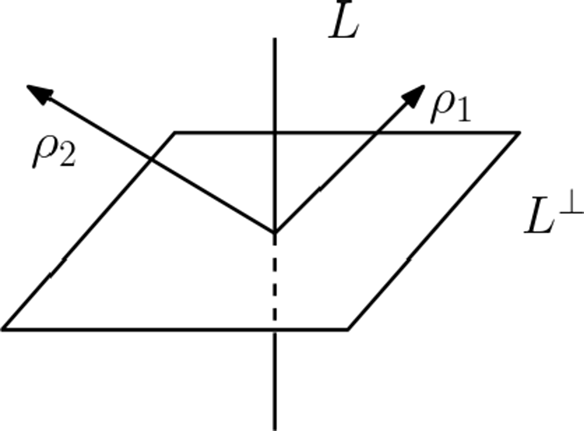


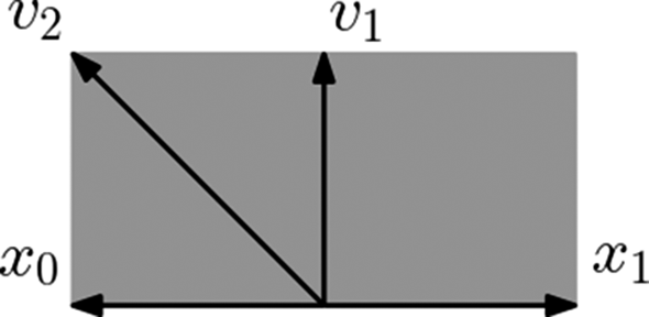

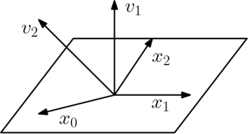

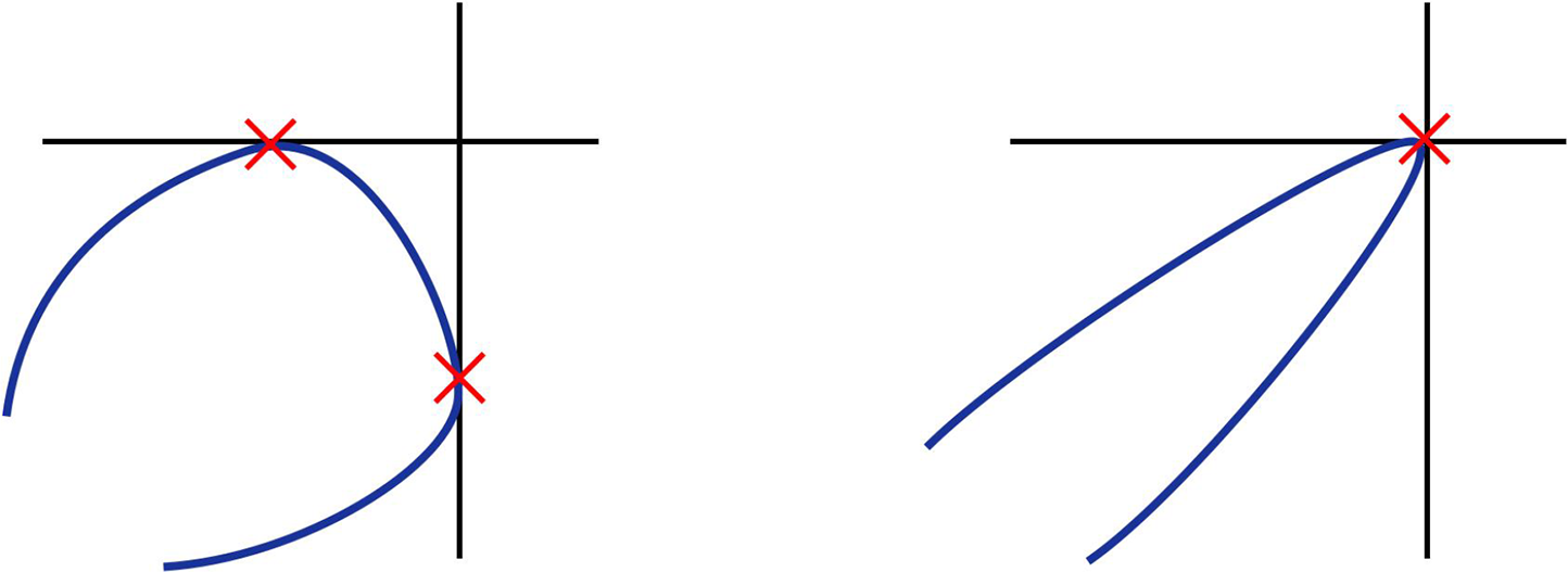

 Open access