





1 Introduction
The primary questions driving research in the social and behavioral sciences aim to uncover cause-and-effect relationships rather than mere associations (Grosz et al., Reference Grosz, Rohrer and Thoemmes2020). Traditionally, randomized experiments have been regarded as the gold standard for drawing causal conclusions in many empirical research fields, including psychology (Rubin, Reference Rubin1974). However, successfully randomizing participants or manipulating the independent variable of interest is often unfeasible, unethical, or impractical in many psychological research contexts. Consequently, while many research questions in psychology implicitly involve causality, researchers must often rely on observational data as their only viable option to draw inferential conclusions (Grosz et al., Reference Grosz, Rohrer and Thoemmes2020).
In causal reasoning, research objectives can generally be divided into related but distinct categories (Shimizu, Reference Shimizu2019). The first involves estimating the magnitude of true causal effects, assuming that one already knows that x causes y. The second is causal structure learning (or causal discovery), where the goal is to uncover the causal structure or determine the directionality of relationships between variables. The research focus in the present study falls into the latter category, aiming to identify whether x causes y.
Learning causal structures from observational data is challenging; hence, the well-known adage correlation does not imply causation. In other words, a correlation between two events does not prove that one event causes the other. Assuming two events are truly correlated, however, it is philosophically implied that the data-generating process involves some form of underlying causal structure that introduces such correlation. According to Reichenbach’s Common Cause Principle (Reichenbach, Reference Reichenbach1956), if two events are correlated, the correlation arises either from a direct causal relationship between the events or from a third factor that generates the correlation, known as a Reichenbachian “common cause” (Hofer-Szabó et al., Reference Hofer-Szabó, Rédei and Szabó2013; Reichenbach, Reference Reichenbach1956).
In the context of causal structure learning, the Reichenbach Common Cause Principle naturally applies in common research scenarios involving two variables of interest (i.e., x and y). If x and y are truly associated (i.e., the association is not due to random or sampling error), at least seven possible causal structures could explain the observed correlation in the data. These seven data-generating models are illustrated as panels (a–g) in Figure 1. Footnote 1 Specifically, the association can be the result of a direct causal relationship between the two variables, that is, (a) x causes y (or in path notation, x → y); (b) y causes x (y → x); or (c) a reciprocal causal structure exists (i.e., x → y and y → x). Alternatively, the observed association may not result from a direct causal relationship but can instead be fully attributed to a (set of) hidden confounder(s), u, as depicted in panel d (i.e., x ← u → y). In addition, the direct causal paths from models (a–c) and hidden confounders (u) can coexist, as shown in models (e–g). For example, in model e, the association between x and y is driven by both: (1) a direct causal path from x to y and (2) a (set of) hidden confounders, u (i.e., x → y and x ← u → y).
A list of possible data-generating models: x is associated with y.

Distinguishing among competing data-generating models is often a central objective in psychological research, even if not explicitly articulated, with the true causal structure between two variables of interest carrying significant theoretical and practical implications. For example, consider loneliness (x) and depression (y). If researchers hypothesize that loneliness causes depression (i.e., in path notation, loneliness → depression, as represented by models a, c, e, or g in Figure 1), targeted interventions can be designed to alleviate depressive symptoms by reducing loneliness. Conversely, when the true data-generating model does not include the loneliness → depression path (e.g., models b, d, or f in Figure 1), interventions focusing solely on loneliness can be expected to be ineffective in ameliorating depressive symptoms.
Unfortunately, competing models cannot be distinguished using commonly employed linear methods that rely on first- and second-order moments (i.e., means, variances, and covariances), such as correlational analysis, linear regression, and structural equation modeling (SEM). When applying these statistical techniques with only x and y being observed, all seven causally competing models presented in Figure 1 are statistically equivalent (or symmetrical) and provide identical representations of the information in the data. In recent years, various causal discovery algorithms (e.g., Hyvärinen et al., Reference Hyvärinen, Karhunen and Oja2001; Mooij et al., Reference Mooij, Peters, Janzing, Zscheischler and Schölkopf2016; Peters et al., Reference Peters, Mooij, Janzing and Schölkopf2014; Shimizu et al., Reference Shimizu, Hoyer, Hyvärinen, Kerminen and Jordan2006) and statistical methods for directional dependence (e.g., Dodge & Rousson, Reference Dodge and Rousson2000; Sungur, Reference Sungur2005; von Eye & DeShon, Reference von Eye and DeShon2012; Wiedermann & von Eye, Reference Wiedermann and von Eye2015; Wiedermann et al., Reference Wiedermann, Li, von Eye, Wiedermann, Kim, Sungur and von Eye2021) have been developed. In contrast to standard methods of associations, these causal learning techniques make use of higher than second order moments (e.g., skewness, kurtosis, co-skewness, and co-kurtosis). These methodological advancements have allowed researchers to investigate the causal structure between variables using observational data.
While many causal discovery algorithms (e.g., Shimizu et al., Reference Shimizu, Inazumi, Sogawa, Hyvärinen, Kawahara, Washio and Bollen2011; Spirtes et al., Reference Spirtes, Glymour and Scheines2001) are designed to explore causal structures in multivariate data involving multiple variables, we focus on bivariate causal discovery within the framework of linear non-Gaussian models (Shimizu et al., Reference Shimizu, Hoyer, Hyvärinen, Kerminen and Jordan2006; Wiedermann et al., Reference Wiedermann, Li, von Eye, Wiedermann, Kim, Sungur and von Eye2021). It is worth noting that, although both aim to infer causal direction and may share underlying statistical foundations,Footnote 2 bivariate causal discovery is not necessarily a special or simpler case of multivariate causal discovery. Specifically, many multivariate causal discovery techniques rely on information from multiple observed variables, such as conditional independencies used in the Peter-Clark (PC) algorithm (Spirtes et al., Reference Spirtes, Glymour and Scheines2001), and therefore, they aim to explore the causal structure for part, if not all, of the underlying network of variables. In contrast, in the bivariate case, such as the research scenario considered in the current study, researchers can only leverage information from the two observed variables. As a result, whereas methods for multivariate causal learning are exploratory in nature for the entire causal network, the bivariate approach is often used as a confirmatory framework for testing specific hypotheses and/or comparing competing theories about the causal directionality between two variables of interest. In this study, we focus on the bivariate case, as it frequently addresses fundamental questions regarding psychological theories, particularly during the early stages of research (cf. Wiedermann & von Eye, Reference Wiedermann and von Eye2025).
Under linear non-Gaussian models, methodologists aim to differentiate causally competing models by leveraging higher-moment information inherent in nonnormally distributed data. Many properties and tests have been developed to uncover the causal structure of the true data-generating model within this context. The associated asymmetry properties that facilitate this identification have been integrated and unified into the comprehensive framework of Direction Dependence Analysis (DDA; Wiedermann & von Eye, Reference Wiedermann and von Eye2025; Wiedermann et al., Reference Wiedermann, Li, von Eye, Wiedermann, Kim, Sungur and von Eye2021).
By applying DDA principles, a subgroup of causally competing models (such as those in Figure 1) can be uniquely identified from the data. Specifically, under the assumption of no unmeasured confounding, DDA leverages higher-order information from observed variables and error terms of fitted linear models to differentiate two causally competing models, such as Model 1a (x → y) and Model 1b (y → x) (Wiedermann & von Eye, Reference Wiedermann and von Eye2025; Wiedermann et al., Reference Wiedermann, Li, von Eye, Wiedermann, Kim, Sungur and von Eye2021). These properties have been validated through analytical derivations, and their performance in finite samples has been evaluated in previous simulation studies (e.g., von Eye & DeShon, Reference von Eye and DeShon2012; Wiedermann & von Eye, Reference Wiedermann and von Eye2015). However, the assumption of no unobserved confounding is rather strict and is often violated in practical scenarios.
To account for the presence of unmeasured confounders (u), more general properties and tests based on the independence of predictors and regression errors have been introduced in the DDA framework (Wiedermann & Sebastian, Reference Wiedermann and Sebastian2020; Wiedermann et al., Reference Wiedermann, Li, von Eye, Wiedermann, Kim, Sungur and von Eye2021). These asymmetry properties enable researchers to distinguish between unconfounded and confounded models. Specifically, it allows one to differentiate among Model 1a (x → y), Model 1b (y → x), and a family of models involving latent confounders (i.e., 1d–1f). When unmeasured confounders (u) are present, however, existing approaches provide limited information about either the presence or the direction of causality between x and y. In other words, causally competing models involving u (i.e., 1d–1f) are indistinguishable using extant methods without imposing additional assumptions (e.g., the assumption that the convolution of hidden confounders follows a normal distribution; Chen & Chan, Reference Chen and Chan2013; Schultheiss et al., Reference Schultheiss, Bühlmann and Yuan2024; Wiedermann, Reference Wiedermann2022; Wiedermann & von Eye, Reference Wiedermann and von Eye2025).
More recently, Shi et al. (Reference Shi, Zhang, Wiedermann and Fairchild2025) proposed an algorithm that shows promise in detecting the directionality of causation in the presence of arbitrarily distributed unmeasured confounders (i.e., distinguishing between Models 1e and 1f). However, the proposed algorithm also relies on additional untenable assumptions: (1) the unobserved confounding is minor and (2) a true causal path exists between x and y. Chen et al. (Reference Chen, Huang, Cai, Hao and Zhang2024) developed a statistical approach to identify causal links between observed variables and then determine their causal direction in the presence of non-Gaussian latent confounder (i.e., distinguishing among Models 1d, 1e, and 1f). The algorithm by Chen et al. (Reference Chen, Huang, Cai, Hao and Zhang2024) relies on higher-order cumulants (at least of the fifth order) and, unsurprisingly, requires very large sample sizes (around 100,000) for acceptable performance.
While the framework of linear non-Gaussian models offers valuable insights into bivariate causal discovery, particularly by enabling researchers to identify causal structures between variables without temporal information (i.e., such as in cross-sectional data), only a subset of causally competing models can be distinguished with current methods. Determining the existence and direction of causal paths becomes particularly challenging in the presence of unmeasured or latent confounders. In real-world observational studies, unmeasured confounders are often the norm rather than the exception (D’Onofrio et al., Reference D’Onofrio, Sjölander, Lahey, Lichtenstein and Öberg2020), significantly limiting the applicability of causal discovery techniques in realistic scenarios commonly encountered in psychological research.
Incorporating temporal order information from longitudinal data can complement existing causal discovery algorithms, by offering additional information on the underlying causal structure that generated the observed variable association. One advantage of using a longitudinal design, widely recognized by psychologists, is its capacity to more effectively test causal hypotheses (Maxwell & Cole, Reference Maxwell and Cole2007; Rutter, Reference Rutter1994). Specifically, a key implicit assumption of longitudinal designs is that an effect always follows its cause in time. Thus, in the context of causal structure learning, when the variables x and y are truly associated, and x is measured earlier in time than y (i.e., when the competing causal path, y → x, can be ruled out on theoretical grounds), integrating temporal order information reduces the number of possible competing causal models from 7 (Figure 1) to 3, as shown in Figure 2.
A list of possible data-generating models: x is associated with y, and x is measured before y.

Temporal information can therefore bring researchers closer to concluding that x causes y (i.e., Models 2a and 2b), as illustrated in Figure 2, though there remains an alternative causal model where the association between x and y is fully explained by unmeasured confounders u (i.e., Model 2c). As discussed earlier, existing non-Gaussian structure learning algorithms can distinguish Model 2a from Models 2b and 2c.Footnote 3 However, Model 2a represents a rather unrealistic scenario, as it assumes that there are no unmeasured confounders between x and y. In most applications, the more crucial (and unresolved) question is how to distinguish between Models 2b and 2c.
In this study, we aim to integrate insights from both distributional information in the data and temporal information over time to address the issue of learning longitudinal causal structures from observational data. Within the framework of linear non-Gaussian models, we introduce statistical theories and corresponding algorithms to test the existence of longitudinal causal paths (i.e., whether x at time 1 causes y at time 2) when unmeasured confounders are present. In contrast to many existing approaches (e.g., Shi et al., Reference Shi, Zhang, Wiedermann and Fairchild2025; Wiedermann et al., Reference Wiedermann, Li, von Eye, Wiedermann, Kim, Sungur and von Eye2021), which view unmeasured confounders as undesirable external factors hampering sound causal conclusions, the algorithm proposed here explicitly leverages the information carried by latent confounders, as we will demonstrate in detail later.
The remainder of this article is organized as follows. First, we derive the statistical theory and propose an algorithm for bivariate longitudinal causal discovery based on joint higher-order cumulants. Next, we evaluate the performance of the proposed algorithm through Monte Carlo simulations (Study I). In Study II, we further examine the factors influencing the behavior of the proposed test statistics, with the aim of explaining the observed statistical power rates and offering guidelines for researchers applying the proposed methods. We then present two empirical examples to illustrate the real-world application of the proposed algorithms with psychological data: the first real-world example uses a cross-sectional design with temporal information provided from retrospective reports; the second example uses a truly longitudinal design. Finally, we conclude with a discussion of the implications of our findings, best-practice recommendations for empirical researchers and potential directions for future research.
2 Non-Gaussian longitudinal causal learning
2.1 Notations and assumptions
For two variables of interest with temporal information, we consider two competing causal models as shown in Figure 3:
-
a. Model I: There is no causal relationship between x and y. Any observed association between x and y is fully explained by the unobserved confounder u (i.e., x ← u → y).
-
b. Model II: x causes y, and both x and y are also caused by the unobserved confounder u (x → y with x ← u → y).
Population causal models considered in the current study.

Assuming that the data-generating mechanism can be approximated by the linear model, the population Model I can be expressed as follows (without loss of generality, the intercept terms are omitted):


where
${\unicode{x3b2}}_1$
 and
${\unicode{x3b2}}_2$
and
${\unicode{x3b2}}_2$
 represent the causal effects from u to x and y, respectively.
${e}_x$
represent the causal effects from u to x and y, respectively.
${e}_x$
 and
${e}_y$
and
${e}_y$
 denote the corresponding error terms for x and y. For Model II, the true data-generating model can be expressed as follows:


where
$\unicode{x3b7}$
 indicates the true causal effect from x to y. Other notations are the same as defined before.
Note that there is only one latent confounder (u) in the above equations. Without loss of generality, however, this global latent confounder (u) can be conceptualized as an additive combination of k independent hidden confounders
${u}_i$
 (i = 1, …, k), representing all possible common causes between x and y (see Figure S1 in the Supplementary Material; Chen & Chan, Reference Chen and Chan2013; Wiedermann & von Eye, Reference Wiedermann and von Eye2025). Importantly, researchers need not assume that the confounders are independent. The reason for this is that, in linear acyclic causal systems, a set of dependent hidden confounders can always be expressed as the linear sum of hidden independent factors (Hoyer et al., Reference Hoyer, Shimizu, Kerminen and Palviainen2008; Shimizu, Reference Shimizu2022).
As a key observation, under linearity, Model II can be viewed as a special case of Model I when
$\unicode{x3b7} =0$
 . Thus, distinguishing between Model I and Model II is equivalent to testing whether
$\unicode{x3b7} =0$
. Thus, distinguishing between Model I and Model II is equivalent to testing whether
$\unicode{x3b7} =0$
 . The two causally competing models cannot be distinguished when fitting a simple linear regression (or SEM) model that relies solely on the first- and second-order moments of the observed data. Specifically, assuming the data-generating model follows Equations (3) and (4), the estimated ordinary least square regression coefficient of the mis-specified model
$y={\unicode{x3b7}}^{\prime }x+{e_y}^{\prime }$
. The two causally competing models cannot be distinguished when fitting a simple linear regression (or SEM) model that relies solely on the first- and second-order moments of the observed data. Specifically, assuming the data-generating model follows Equations (3) and (4), the estimated ordinary least square regression coefficient of the mis-specified model
$y={\unicode{x3b7}}^{\prime }x+{e_y}^{\prime }$
 (i.e., the model that erroneously ignores the presence of u) can be expressed as
$\widehat{\unicode{x3b7}^{\prime }}\overset{p}{\to}\frac{Cov\left(x,y\right)}{Var(x)}=\unicode{x3b7} +\frac{\unicode{x3b2}_1{\unicode{x3b2}}_2\mathit{{var}}(u)}{{\unicode{x3b2}_1}^2\mathit{{var}}(u)+\mathit{{var}}\left({e}_x\right)}$
(i.e., the model that erroneously ignores the presence of u) can be expressed as
$\widehat{\unicode{x3b7}^{\prime }}\overset{p}{\to}\frac{Cov\left(x,y\right)}{Var(x)}=\unicode{x3b7} +\frac{\unicode{x3b2}_1{\unicode{x3b2}}_2\mathit{{var}}(u)}{{\unicode{x3b2}_1}^2\mathit{{var}}(u)+\mathit{{var}}\left({e}_x\right)}$
 . As a consequence, the estimated slope
$\widehat{\eta}$
. As a consequence, the estimated slope
$\widehat{\eta}$
 will always be nonzero, regardless of its true population value, unless either
${\unicode{x3b2}}_1$
will always be nonzero, regardless of its true population value, unless either
${\unicode{x3b2}}_1$
 or
${\unicode{x3b2}}_2$
or
${\unicode{x3b2}}_2$
 are zero (i.e., in the absence of u).
Building on the notations introduced above, we make the following additional assumptions to facilitate detecting the presence of longitudinal causal effects from x to y within the linear non-Gaussian framework.
(A1). Temporal order. Observed variable x precedes y (i.e., the reverse causal path y → x is not permitted).
(A2). Linearity. The relationships between all variables are linear.
(A3).
Independence.
$\ {e}_x$
 and
$ {e}_y$
and
$ {e}_y$
 are additive error terms with zero means and constant variances that are independent of u and of each other, that is,
${e}_x\perp {e}_y$
are additive error terms with zero means and constant variances that are independent of u and of each other, that is,
${e}_x\perp {e}_y$
 ,
${e}_x\perp u$
,
${e}_x\perp u$
 , and
${e}_y\perp u$
, and
${e}_y\perp u$
 .
.
(A4).
Presence of a hidden confounder.
There exist hidden factors (
${u}_i$
 ) that cause both x and y. For
$i>1$
) that cause both x and y. For
$i>1$
 , multiple hidden factors
${u}_i$
, multiple hidden factors
${u}_i$
 can be represented by a global hidden component u. In the presence of u,
${\unicode{x3b2}}_1\ne 0$
can be represented by a global hidden component u. In the presence of u,
${\unicode{x3b2}}_1\ne 0$
 and
${\unicode{x3b2}}_2\ne 0$
and
${\unicode{x3b2}}_2\ne 0$
 .
.
(A5).
Nonnormality. Both u and
${e}_x$
 are nonnormally distributed.Footnote
4
are nonnormally distributed.Footnote
4
Here, Assumption (A5) is in sharp contrast to the distributional assumptions routinely made in standard second-order moment-based methods of association. While OLS regression and SEMs usually rely on the assumption that variables follow a normal distribution, the methods presented here rest on the assumption that variables deviate from normality. This requirement is justifiable from both, an empirical and a theoretical perspective. From an empirical perspective, nonnormality of variables constitutes a phenomenon that is ubiquitous across the empirical sciences (see, e.g., Blanca et al. Reference Blanca, Arnau, López-Montiel, Bono and Bendayan2013; Micceri, Reference Micceri1989), suggesting that the requirement of nonnormality can be expected to be fulfilled in practice.
From a theoretical perspective, the ubiquitousness of nonnormality can be explained using Cramér’s decomposition theorem (Cramér, Reference Cramér1970), stating that when the sum of two independent real-values variates follows a normal distribution, both summand variates must follow a normal distribution as well. This holds accordingly for more than two independent variables, that is, when the sum of many finite independent variables follows a normal distribution, then all independent variables must be normal. As a consequence, the sum of independent variables cannot be exactly normal, except all independent summands are exactly normal (known as the linear closure property of the normal distribution; see, e.g., Glymour et al., Reference Glymour, Zhang and Spirtes2019). Since this strict requirement is likely to be violated in real-world settings, nonnormality can be expected to be omnipresent in practice.
It should be noted that Cramér’s decomposition theorem is not in conflict with the central limit theorem (CLT), which is well known among psychologists.Footnote 5 Specifically, under the Lyapunov condition (Lyapunov, Reference Lyapunov1901), the sum of independent variables converges to a normal distribution as the number of variables approaches infinity. However, with a finite number of variables (e.g., independent confoundersFootnote 6 ), the sum may come close to the normal distribution but will never be exactly normally distributed. Moreover, the rate of convergence to normality can be slow, particularly when the independent variables have large third moments (Zhang et al., Reference Zhang, Astivia, Kroc and Zumbo2023). Note that the number of potential confounders never reaches infinity in practice. In most clinical or psychological applications, the number of potential confounders is typically moderate to small. For example, Pocock et al. (Reference Pocock, Collier, Dandreo, de Stavola, Goldman, Kalish and McCormack2004) reviewed 73 articles in observational epidemiology and found that the median number of potential confounders was 7.
While we believe the assumption of nonnormality is quite realistic, given both empirical evidence and theoretical justifications via Cramér’s decomposition theorem, a practical question is whether the variables exhibit enough nonnormality to yield adequate statistical power when implementing the proposed algorithm, as we will demonstrate later in this article. From a practical perspective, justification may draw on prior theory regarding factors such as the number of potential confounders and the degree of their skewness. In addition, we would like to emphasize that, in the theoretical framework, we conceptualize u as a global latent (or hidden) construct of hidden confounding influences not considered in the analysis. This issue of approximate normality can be addressed at the research design stage. For instance, researchers may collect information on major confounders guided by substantive theory and adjust for selected confounders in the data analysis. Consequently, the set of latent (hidden) confounders u decreases with the number of observed confounding covariates which, in turn, can decrease the “Gaussianization effect” of u. This way, data situations can be constructed based on a limited number of confounders, possibly as few as one, that are expected to be strongly nonnormal by design. In addition, incorporating various measured confounders may also serve as a tool for sensitivity analysis of the proposed algorithm, helping to evaluate the robustness of its assumptions and the stability of the causal conclusions.
Under Assumptions (A1)–(A5), we can derive properties and tests to examine the presence of the longitudinal causal path (
$\unicode{x3b7}$
 ) using marginal and joint higher cumulants (Chen & Chan, Reference Chen and Chan2013; Chen et al., Reference Chen, Huang, Cai, Hao and Zhang2024; Hyvärinen & Smith, Reference Hyvärinen and Smith2013; Wiedermann, Reference Wiedermann2022). Before we present the main theoretical results, we briefly review basic properties of cumulants.
2.2 Cumulants
Cumulants are a set of descriptive constants of a given (joint) probability distribution that are, from a theoretical perspective, sometimes more useful than moments (Stuart & Ord, Reference Stuart and Ord1987).
Definition 1
(Joint cumulants)
(Brillinger, Reference Brillinger2001). Let
$\mathbf{X}=\left({X}_1,{X}_2,\dots {X}_{\mathrm{n}}\right)$
 be a random vector of length n. The joint cumulants are formally defined as partial derivatives of the joint cumulant generating function (cgf) at zero and are denoted as follows:

The joint cgf of X is given by

where
${M}_X(t)=\mathbb{E}\left[\exp (tX)\right]$
 is the joint moment generating function (mgf).
Footnote
7
is the joint moment generating function (mgf).
Footnote
7
By taking the coefficients of the Taylor series expansion of
${\unicode{x3ba}}_X(t)$
 , the joint cumulants of X can be then evaluated using the following function (Brillinger, Reference Brillinger2001):

where P is the set of all partitions of the set
$\left\{1,2,\dots k\right\}$
 ,
$\left|\pi \right|$
,
$\left|\pi \right|$
 is the number of blocks in the partition
$\pi$
is the number of blocks in the partition
$\pi$
 , and B is the block in the partition
$\pi$
, and B is the block in the partition
$\pi$
 .
.
For convenience, we use
${Cum}_i(x)$
 to denote the ith order cumulants for a single variable x and
$Cum\left(x,x,\dots, y,y,\dots \right)$
to denote the ith order cumulants for a single variable x and
$Cum\left(x,x,\dots, y,y,\dots \right)$
 to indicate joint cumulants involving two variables. For example,
${Cum}_3(x)$
to indicate joint cumulants involving two variables. For example,
${Cum}_3(x)$
 and
${Cum}_4(x)$
and
${Cum}_4(x)$
 refer to the third- and fourth-order (marginal) cumulants describing the skewness and excess-kurtosis of x,
$Cum\left(x,x,y\right)$
refer to the third- and fourth-order (marginal) cumulants describing the skewness and excess-kurtosis of x,
$Cum\left(x,x,y\right)$
 and
$Cum\left(x,y,y\right)$
and
$Cum\left(x,y,y\right)$
 describe the third-order (joint) cumulants, and
$Cum\left(x,x,x,y\right)$
describe the third-order (joint) cumulants, and
$Cum\left(x,x,x,y\right)$
 ,
$Cum\left(x,y,y,y\right)$
,
$Cum\left(x,y,y,y\right)$
 , and
$Cum\left(x,x,y,y\right)$
, and
$Cum\left(x,x,y,y\right)$
 describe the fourth-order (joint) cumulants of x and y. For simplicity and without restricting generality, the observed variables x and y are hereinafter assumed to be standardized. All variables in the system are expressed in mean-centered form (mean = 0).
Lemma 1. Under Model II (defined by Equations (3) and (4) and Assumptions (A2)–(A5), we obtain the following results for the third- and fourth-order joint cumulants of observed variables x and y:


A proof for Lemma 1 is given in Appendix A. Note that under Model I, that is, when
$\unicode{x3b7} =0$
 , joint cumulants simplify to


In the following section, we make use of these higher-order cumulants to develop measures for the presence of longitudinal causal paths under hidden confounding.
2.3 Measures for the presence of a longitudinal causal path (
$\boldsymbol{\unicode{x3b7}}$
 )
)

Using the results from Lemma 1, we derive the following theorems.
Theorem 1. Let
${\Delta }_1= Cum\left(x,x,x,y\right)\times Cum\left(x,y,y,y\right)-{\left[ Cum\left(x,x,y,y\right)\right]}^2$
 . If no true causal effect from x to y exists (i.e.,
$\unicode{x3b7} =0$
. If no true causal effect from x to y exists (i.e.,
$\unicode{x3b7} =0$
 ), we have
${\Delta }_1=0$
), we have
${\Delta }_1=0$
 . If x truly causes y (
$\unicode{x3b7} \ne 0$
. If x truly causes y (
$\unicode{x3b7} \ne 0$
 ), with the faithfulness assumption that
$\unicode{x3b7} \ne -\frac{\unicode{x3b2}_2}{\unicode{x3b2}_1}$
), with the faithfulness assumption that
$\unicode{x3b7} \ne -\frac{\unicode{x3b2}_2}{\unicode{x3b2}_1}$
 , we have
${\Delta }_1\ne 0$
, we have
${\Delta }_1\ne 0$
 .
.
Corresponding Proof. Given Equations (10)–(12), we obtain

By setting
${\Delta }_1=0$
 and simplifying the result, we obtain the following quadratic equation for
$\eta$
and simplifying the result, we obtain the following quadratic equation for
$\eta$
 , assuming
${Cum}_4(u)\ne 0$
, assuming
${Cum}_4(u)\ne 0$
 ,
${Cum}_4\left({e}_x\right)\ne 0$
,
${Cum}_4\left({e}_x\right)\ne 0$
 ,
${\unicode{x3b2}}_1\ne 0,$
,
${\unicode{x3b2}}_1\ne 0,$
 and
${\unicode{x3b2}}_2\ne 0$
and
${\unicode{x3b2}}_2\ne 0$
 :
:

Solving Equation (19) for
$\eta$
 , the only two solutions are

Therefore, when
$\unicode{x3b7} =0$
 , it follows that
${\Delta }_1=0$
, it follows that
${\Delta }_1=0$
 and, assuming faithfulness holds (i.e.,
$\unicode{x3b7} \ne -\frac{\unicode{x3b2}_2}{\unicode{x3b2}_1}$
and, assuming faithfulness holds (i.e.,
$\unicode{x3b7} \ne -\frac{\unicode{x3b2}_2}{\unicode{x3b2}_1}$
 ), when
$\unicode{x3b7} \ne 0$
), when
$\unicode{x3b7} \ne 0$
 , then
${\Delta }_1\ne 0$
, then
${\Delta }_1\ne 0$
 .
.
It should be noted that by utilizing information based on higher-order cumulants, our method is related to prior work in causal discovery (e.g., Chen & Chan, Reference Chen and Chan2013; Chen et al., Reference Chen, Huang, Cai, Hao and Zhang2024), although the research goals and algorithms differ in several important ways. For instance, the same analytic result in Theorem 1 was also used by Chen et al. (Reference Chen, Huang, Cai, Hao and Zhang2024) as the first step (i.e., Case 1) in their causal learning algorithm. In addition, Chen et al. (Reference Chen, Huang, Cai, Hao and Zhang2024) provided and proved a more general result based on joint cumulants of fourth order or higher (see their Theorem 3). A more detailed comparison between our algorithm and other cumulant-based causal learning methods is presented later in the article.
In a similar manner, using Equations (8)–(12), we can derive two additional theorems by utilizing both third- and fourth-order joint cumulants as follows.
Theorem 2
. Let
${\Delta }_2= Cum\left(x,x,y\right)\times Cum\left(x,x,y,y\right)- Cum\left(x,y,y\right)\times Cum\left(x,x,x,y\right)$
 . When no true causal effect from x to y exists (i.e.,
$\unicode{x3b7} =0$
. When no true causal effect from x to y exists (i.e.,
$\unicode{x3b7} =0$
 ), one obtains
${\Delta }_2=0$
), one obtains
${\Delta }_2=0$
 . When x truly causes y (
$\unicode{x3b7} \ne 0$
. When x truly causes y (
$\unicode{x3b7} \ne 0$
 ), with the faithfulness assumption that
$\unicode{x3b7} \ne -\frac{\unicode{x3b2}_2}{\unicode{x3b2}_1}$
), with the faithfulness assumption that
$\unicode{x3b7} \ne -\frac{\unicode{x3b2}_2}{\unicode{x3b2}_1}$
 , one obtains
${\Delta }_2\ne 0$
, one obtains
${\Delta }_2\ne 0$
 .
.
The corresponding proof for Theorem 2 is given in Appendix B.
Theorem 3
. Let
${\Delta }_3= Cum\left(x,x,y\right)\times Cum\left(x,y,y,y\right)- Cum\left(x,y,y\right)\times Cum\left(x,x,y,y\right)$
 . When no true causal effect from x to y exists (i.e.,
$\unicode{x3b7} =0$
. When no true causal effect from x to y exists (i.e.,
$\unicode{x3b7} =0$
 ), one obtains
${\Delta }_3=0$
), one obtains
${\Delta }_3=0$
 . When x truly causes y (
$\eta \ne 0$
. When x truly causes y (
$\eta \ne 0$
 ), with the faithfulness assumption that
$\unicode{x3b7} \ne -\frac{\unicode{x3b2}_2}{\unicode{x3b2}_1}$
), with the faithfulness assumption that
$\unicode{x3b7} \ne -\frac{\unicode{x3b2}_2}{\unicode{x3b2}_1}$
 and
$\unicode{x3b7} \ne -\frac{Cum_4(u){Cum}_3\left({e}_x\right){\unicode{x3b2}}_2}{Cum_4(u){Cum}_3\left({e}_x\right){\unicode{x3b2}}_1-{Cum}_3(u){Cum}_4\left({e}_x\right)}$
and
$\unicode{x3b7} \ne -\frac{Cum_4(u){Cum}_3\left({e}_x\right){\unicode{x3b2}}_2}{Cum_4(u){Cum}_3\left({e}_x\right){\unicode{x3b2}}_1-{Cum}_3(u){Cum}_4\left({e}_x\right)}$
 , one obtains
${\Delta }_3\ne 0$
, one obtains
${\Delta }_3\ne 0$
 .
.
The corresponding proof for Theorem 3 is given in Appendix C.
With the assumptions stated above and
$n\to \infty$
 , all three test statistics (
${\Delta }_1,{\Delta }_2,\mathrm{and}\;{\Delta }_3$
, all three test statistics (
${\Delta }_1,{\Delta }_2,\mathrm{and}\;{\Delta }_3$
 ) can be used to detect the presence of a direct causal path from x to y. Specifically,
$\unicode{x3b7} \ne 0$
) can be used to detect the presence of a direct causal path from x to y. Specifically,
$\unicode{x3b7} \ne 0$
 finds empirical support when
${\Delta }_1\ne 0$
finds empirical support when
${\Delta }_1\ne 0$
 ,
${\Delta }_2\ne 0,\mathrm{or}\;{\Delta }_3\ne 0$
,
${\Delta }_2\ne 0,\mathrm{or}\;{\Delta }_3\ne 0$
 . In finite samples where only x and y are observed, the test statistics
${\Delta }_1,{\Delta }_2,\mathrm{and}\;{\Delta }_3$
. In finite samples where only x and y are observed, the test statistics
${\Delta }_1,{\Delta }_2,\mathrm{and}\;{\Delta }_3$
 can be computed using the sample joint cumulants estimated from Equation (7). In addition, statistical significance tests can be performed using 100(1 − α) % nonparametric bootstrapping confidence intervals (Davison & Hinkley, Reference Davison and Hinkley1997).
A key point to recognize is that
${\Delta }_1$
 relies solely on the fourth-order joint cumulants and presupposes nonzero marginal fourth-order cumulants for both u and
${e}_x$
relies solely on the fourth-order joint cumulants and presupposes nonzero marginal fourth-order cumulants for both u and
${e}_x$
 . In contrast, both
${\Delta }_2$
. In contrast, both
${\Delta }_2$
 and
${\Delta }_3$
and
${\Delta }_3$
 incorporate third- and fourth-order joint cumulants, requiring the existence of third-order cumulants (i.e., skewness) for u and
${e}_x$
incorporate third- and fourth-order joint cumulants, requiring the existence of third-order cumulants (i.e., skewness) for u and
${e}_x$
 . In this sense,
${\Delta }_1$
. In this sense,
${\Delta }_1$
 is regarded as a more general test that relies on fewer assumptions. However, by incorporating third-order information when available, using
${\Delta }_2$
is regarded as a more general test that relies on fewer assumptions. However, by incorporating third-order information when available, using
${\Delta }_2$
 and
${\Delta }_3$
and
${\Delta }_3$
 offers incremental power to detect the presence of
$\eta$
offers incremental power to detect the presence of
$\eta$
 . Furthermore, even when the third-order cumulants are zero, both
${\Delta }_2$
. Furthermore, even when the third-order cumulants are zero, both
${\Delta }_2$
 and
${\Delta }_3$
and
${\Delta }_3$
 are expected to be zero (as shown in Equations B2 and C2), which does not necessarily lead to incorrect conclusions, particularly within the framework of the multiple testing algorithm introduced in the following section.
2.4 Operationalizing a multiple testing algorithm
We proposed three test statistics (
${\Delta }_1,{\Delta }_2,\mathrm{and}\;{\Delta }_3$
 ) for evaluating the presence of a nonzero direct causal effect
$\eta$
) for evaluating the presence of a nonzero direct causal effect
$\eta$
 . In finite samples, the statistical power to detect a true effect (
$\eta \ne 0$
. In finite samples, the statistical power to detect a true effect (
$\eta \ne 0$
 ) is expected to be influenced by two primary factors: the sample size (n) and the absolute magnitudes of the test statistics (
${\Delta }_1,{\Delta }_2,\mathrm{and}\;{\Delta }_3$
) is expected to be influenced by two primary factors: the sample size (n) and the absolute magnitudes of the test statistics (
${\Delta }_1,{\Delta }_2,\mathrm{and}\;{\Delta }_3$
 ). As shown in the previous section, the magnitudes of these test statistics can be expected to be influenced by the complex interplay of several parameters, including
${Cum}_4(u),{Cum}_4\left({e}_x\right),{Cum}_3(u),{Cum}_3\left({e}_x\right)$
). As shown in the previous section, the magnitudes of these test statistics can be expected to be influenced by the complex interplay of several parameters, including
${Cum}_4(u),{Cum}_4\left({e}_x\right),{Cum}_3(u),{Cum}_3\left({e}_x\right)$
 ,
${\unicode{x3b2}}_1$
,
${\unicode{x3b2}}_1$
 , and
${\unicode{x3b2}}_2$
, and
${\unicode{x3b2}}_2$
 . Therefore, each test statistic is expected to exhibit greater sensitivity to detect
$\eta$
. Therefore, each test statistic is expected to exhibit greater sensitivity to detect
$\eta$
 for a given combination of these parameters. In practice, the values of the above parameters are unknown, given that u is unobserved. To achieve higher statistical power, we recommend using all three test statistics in conjunction within a multiple testing algorithm, as described below.

Long description
A multiple testing algorithm presented in a numbered list.
* Step 1. Set the significance level alpha and apply the Bonferroni correction for multiple testing using the adjusted alpha prime equals alpha all over 3.
* Step 2. Standardize the observed variables x and y in subsequent analyses.
* Step 3. Compute Delta sub 1, and obtain the 100 times open parenthesis 1 minus alpha prime close parenthesis percent percentile bootstrapping confidence interval, open bracket Delta sub 1 super L, Delta sub 1 super U close bracket.
* Step 4. Compute Delta sub 2, and obtain the 100 times open parenthesis 1 minus alpha prime close parenthesis percent percentile bootstrapping confidence interval, open bracket Delta sub 2 super L, Delta sub 2 super U close bracket.
* Step 5. Compute Delta sub 3, and obtain the 100 times open parenthesis 1 minus alpha prime close parenthesis percent percentile bootstrapping confidence interval, open bracket Delta sub 3 super L, Delta sub 3 super U close bracket.
* Step 6. If 0 is not an element of open bracket Delta sub 1 super L, Delta sub 1 super U close bracket or 0 is not an element of open bracket Delta sub 2 super L, Delta sub 2 super U close bracket or 0 is not an element of open bracket Delta sub 3 super L, Delta sub 3 super U close bracket, then select x yields y. Otherwise, fail to detect the presence of a direct causal path.
3 Study I: Assessing the performance of the proposed algorithm
3.1 Data generation
We conducted Monte Carlo simulations to evaluate the performance of the proposed algorithm in the context of longitudinal bivariate causal discovery with unmeasured confounders. We generated data from a linear non-Gaussian model, where the population model is the same as the one presented in Figure 3b. Specifically, the variables of interest include x and y, and we assumed a temporal order such that x occurs before y. Both x and y share a common cause (confounder), u. All exogenous variables (i.e., u) and error terms for the endogenous variables (i.e., x and y) were generated from various Gamma distributions. Since the research goal is to determine the existence of the causal effect from x to y (i.e., x → y), the effect size of the true causal path (
$\eta$
 ) was manipulated as a key factor of the simulation design, with details discussed below. We also manipulated the sample size, the distribution of the hidden confounder (u), the distribution of the error term (
${e}_x$
) was manipulated as a key factor of the simulation design, with details discussed below. We also manipulated the sample size, the distribution of the hidden confounder (u), the distribution of the error term (
${e}_x$
 ), and the effect size of β1 and β2 paths. Linear transformations were applied to the generated endogenous variables and error terms, so that all population path coefficients in the simulation reflect standardized metrics.
Sample size (N). Four levels of sample sizes were considered, including N = 2,000, 5,000, 10,000, and 50,000. It is worth noting that to accurately estimate higher-order statistics beyond the first and second moments, a larger sample size is generally required (Chan et al., Reference Chan, Chen, Li, Wong and Yau2020). The selection of these sample sizes represents a range from small to large samples for causal discovery under linear non-Gaussian models (Chen et al., Reference Chen, Huang, Cai, Hao and Zhang2024; Shi et al., Reference Shi, Fairchild and Wiedermann2023; Shimizu et al., Reference Shimizu, Hoyer, Hyvärinen, Kerminen and Jordan2006; Tramontano et al., Reference Tramontano, Kivva, Salehkaleybar, Drton and Kiyavash2024).
Distribution of the hidden confounder (u). The latent confounder u was generated from a Gamma distribution, with the scale parameter fixed at 1 and the shape parameter manipulated to create three levels of population skewness, 0.75, 1.50, and 2.25, mimicking mild, moderate, and highly skewed distributions. These distributional choices align with previous simulation studies in causal learning (Shi et al., Reference Shi, Fairchild and Wiedermann2023; Wiedermann & Li, Reference Wiedermann and Li2020).
Distribution of the error term (
${e}_x$
 ). The error term of x (
${e}_x$
). The error term of x (
${e}_x$
 ) was generated from a Gamma distribution with three levels of population: 0.75, 1.50, and 2.25. For simplicity, the error term of y (
${e}_y$
) was generated from a Gamma distribution with three levels of population: 0.75, 1.50, and 2.25. For simplicity, the error term of y (
${e}_y$
 ) was set to follow the same distribution as
${e}_x$
) was set to follow the same distribution as
${e}_x$
 .
.
Effect size of
$\unicode{x3b7}$
 .
The x → y path represents the true longitudinal causal effect of interest. Four levels of effect size for
$\unicode{x3b7}$
.
The x → y path represents the true longitudinal causal effect of interest. Four levels of effect size for
$\unicode{x3b7}$
 were considered: 0, 0.14, 0.39, and 0.59. These population parameters were chosen to represent scenarios with no causal effect between x and y, as well as true causal effects ranging from small to large effect sizes (Cohen, Reference Cohen1988).
Effect sizes of the β1 and β2. The strength of the confounder was manipulated by altering the effect sizes of the β1 and β2 paths. For each path, three effect sizes were considered: 0.14, 0.39, and 0.59, representing small, medium, and larger confounder effects. These levels were fully crossed for the two paths, resulting in nine unique combinations.
In total, 1,296 (4 × 3 × 3 × 4 × 9) simulation conditions were considered. Note that 36 conditions were not included because they were inadmissible (i.e., conditions with
${\unicode{x3b2}}_1$
 =
${\unicode{x3b2}}_2$
=
${\unicode{x3b2}}_2$
 =
$\unicode{x3b7}$
=
$\unicode{x3b7}$
 = 0.59, which yields a negative error variance). Therefore, the final number of simulated conditions was 1,296 – 36 = 1,260. For each simulation condition, 1,000 replications were generated using R 4.1.2 (R Core Team, 2025).
3.2 Data analyses and outcome variables
For each simulated data set, we conducted joint-cumulant-based tests, that is, Δ1, Δ2, and Δ3, to detect the presence of the x → y path. Statistical inferences were drawn based on the 100(1 − α) % percentile bootstrapping confidence intervals with 2,000 resamples. Conclusions were based on the multiple-testing algorithm described in the previous section. That is, a nonzero causal effect was confirmed, when at least one of the three test statistics significantly differed from zero. To control for Type I error rates due to multiple testing, the Bonferroni correction (Bonferroni, Reference Bonferroni1936) was applied. Specifically, for α = 0.05 with a Bonferroni correction (
${\unicode{x3b1}}^{\prime }=0.05/3$
 ), 98.33% bootstrap confidence intervals were constructed.
Using the proposed multiple-testing algorithm, two possible decisions can be made: (1) x causes y and (2) there is no evidence that x causes y. For each simulation condition, we computed the proportions of these decisions across replications. As the outcome measure, we reported the proportion of cases concluding that x causes y (x → y) across simulation conditions. Note that the proportions represent Type I error rates when
$\unicode{x3b7}$
 = 0, whereas for conditions where
$\unicode{x3b7}$
= 0, whereas for conditions where
$\unicode{x3b7}$
 ≠ 0, proportions indicate power rates for detecting the presence of a true causal path x → y. The Type I error rates across simulated conditions (i.e., when η = 0) are summarized in Table 1. The power rates to detect a true causal path from x to y (i.e., when η ≠ 0) are reported in Tables 2–4.
Type I error rates in percent for detecting the causal path x → y (
$\unicode{x3b7}$
 = 0)
= 0)

Table 1 Long description
The table presents Type I error rates for the causal path x yields y where beta sub 7 equals 0.
Column Structure:
* The first three columns define the parameters: Skewness of e sub x (0.75, 1.50, 2.25), beta sub 2 (0.14, 0.39, 0.59), and beta sub 1 (0.14, 0.39, 0.59).
* The remaining columns are grouped into three main sections based on the Skewness of u: 0.75, 1.50, and 2.25.
* Each Skewness of u section is further divided by sample size N: 2,000, 5,000, 10,000, and 50,000.
Row Data Trends:
* For Skewness of e sub x at 0.75, error rates are generally low (0.0 to 1.0) when beta values are low, but increase up to 6.6 as beta sub 1 and beta sub 2 increase to 0.59.
* For Skewness of e sub x at 1.50, error rates show a similar upward trend with higher beta values, reaching a maximum of 8.6 at N equals 10,000 when beta sub 1 and beta sub 2 are 0.59.
* For Skewness of e sub x at 2.25, the highest error rates are observed, peaking at 8.4 for Skewness of u equals 1.50 and N equals 10,000.
* Across all categories, Type I error rates tend to be higher when both beta sub 1 and beta sub 2 are at their maximum value of 0.59, regardless of the skewness of u or sample size N.
Power rates in percent for detecting the causal path x → y (
$\unicode{x3b7}$
 = 0.14)
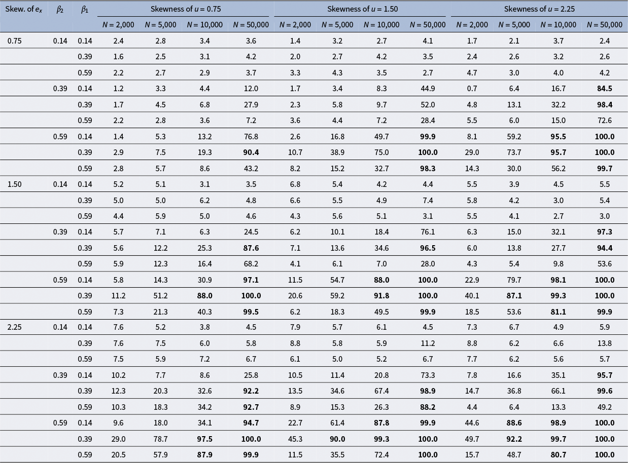
Table 2 Long description
The table presents power rates for detecting the causal path x yields y with a fixed effect size of 0.14.
Vertical Hierarchy:
* The primary row variable is Skewness of e sub x, with levels 0.75, 1.50, and 2.25.
* Within each skewness level, there are sub-rows for beta sub 2 (0.14, 0.39, 0.59).
* Within each beta sub 2 level, there are sub-rows for beta sub 1 (0.14, 0.39, 0.59).
Horizontal Hierarchy:
* The columns are grouped by Skewness of u (0.75, 1.50, and 2.25).
* Under each Skewness of u group, there are four sample size columns: N = 2,000, N = 5,000, N = 10,000, and N = 50,000.
Key Data Trends:
* Power rates generally increase as sample size N increases.
* Power rates are highest when Skewness of e sub x and beta sub 2 are at their maximum values (0.59 and 2.25 respectively).
* Bolded values indicate power rates above 80 percent. For example, at Skewness of e sub x = 0.75, beta sub 2 = 0.39, beta sub 1 = 0.39, and Skewness of u = 2.25, the power reaches 98.4 percent at N = 50,000.
* At the highest settings (Skewness of e sub x = 2.25, beta sub 2 = 0.59, beta sub 1 = 0.39), power reaches 100.0 percent for N = 5,000 and above across all Skewness of u categories.
Note: Power rates above 80% are highlighted in bold.
Power rates in percent for detecting the causal path x → y (
$\unicode{x3b7}$
 = 0.39)

Table 3 Long description
Fallback
Note: Power rates above 80% are highlighted in bold.
Power rates in percent for detecting the causal path x → y (
$\unicode{x3b7}$
 = 0.59)

Table 4 Long description
The table presents power rates for detecting a causal path where gamma equals 0.59.
Column Structure:
* The first three columns define the parameters: Skewness of e sub x (0.75, 1.50, 2.25), beta sub 2 (0.14, 0.39, 0.59), and beta sub 1 (0.14, 0.39, 0.59).
* The remaining columns are grouped into three main sections based on the Skewness of u: 0.75, 1.50, and 2.25.
* Each skewness section is further divided by sample size N: 2,000, 5,000, 10,000, and 50,000.
Data Trends:
* Power rates generally increase as the sample size N increases from 2,000 to 50,000.
* Higher values of beta sub 1 and beta sub 2 correlate with higher power rates.
* Power rates above 80 percent are highlighted in bold, appearing most frequently at N equals 10,000 and N equals 50,000.
* For Skewness of e sub x at 0.75, beta sub 2 at 0.39, and beta sub 1 at 0.39, the power reaches 100.0 at N equals 50,000 when Skewness of u is 1.50 or 2.25.
* Some cells for beta sub 1 and beta sub 2 at 0.59 are marked with dashes, indicating no data or inapplicable conditions.
Note: Power rates above 80% are highlighted in bold.
3.3 Results: Type I error rates
As shown in Table 1, the Type I error rates of the proposed multiple-testing algorithm were well-controlled under the simulated conditions. Across the 324 conditions with
$\unicode{x3b7}$
 = 0, the Type I error rates ranged from 0% to 8.6%. Only three simulation conditions with relatively small sample sizes (i.e., N < 5,000) produced Type I error rates marginally above the 7.5% criterion suggested by Bradley (Reference Bradley1978). Thus, we conclude that researchers using the proposed algorithm face a low risk of falsely concluding that x causes y when no true causal path exists, particularly in large-sample contexts.
3.4 Results: Power rates
As shown in Tables 2–4, under conditions where x is truly a cause of y (i.e., η ≠ 0), the proposed multiple-testing algorithm can successfully detect the presence of the causal path of x → y. The power rates for detecting a true causal path varied across simulation conditions. Below, we summarize the main factors that drive power rates.
First, not surprisingly, the power to detect the true causal path (η) increased with the sample size. For example, as indicated in Table 2, when the population skewness of the latent confounder (u) was 1.50 and the population skewness of
${e}_x$
 was 0.75, with N = 2,000,
${\unicode{x3b2}}_1=0.14$
was 0.75, with N = 2,000,
${\unicode{x3b2}}_1=0.14$
 , and
${\unicode{x3b2}}_2=0.59$
, and
${\unicode{x3b2}}_2=0.59$
 , the power to detect a causal x → y path of
$\unicode{x3b7}$
, the power to detect a causal x → y path of
$\unicode{x3b7}$
 = 0.14 was only 10.7 %. Keeping all other factors the same, the power increased to 38.9%, 75.0%, and 100% as the sample size increased to 5,000, 10,000, and 50,000, respectively.
Second, the power rates to detect the x → y path generally increased with the true effect size (
$\unicode{x3b7}$
 ). For example, when the population skewness of u = 0.75, the population skewness of
${e}_x$
). For example, when the population skewness of u = 0.75, the population skewness of
${e}_x$
 = 0.75,
${\unicode{x3b2}}_1={\unicode{x3b2}}_2=$
= 0.75,
${\unicode{x3b2}}_1={\unicode{x3b2}}_2=$
 0.39, and N = 50,000, the power rates were 27.9%, 63.9%, and 88.0% for
$\unicode{x3b7} =$
0.39, and N = 50,000, the power rates were 27.9%, 63.9%, and 88.0% for
$\unicode{x3b7} =$
 0.14,
$\unicode{x3b7} =$
0.14,
$\unicode{x3b7} =$
 0.39, and
$\unicode{x3b7} =$
0.39, and
$\unicode{x3b7} =$
 0.59, respectively.
Third, the power rates were related to the strength of the latent confounder, particularly the magnitude of
${\unicode{x3b2}}_2$
 (i.e., the u → y path). For instance, as demonstrated in Table 3, when the population skewness of the latent confounder (u) was 1.50, the population skewness of the
${e}_x$
(i.e., the u → y path). For instance, as demonstrated in Table 3, when the population skewness of the latent confounder (u) was 1.50, the population skewness of the
${e}_x$
 was 2.25, with a relatively small sample size of N = 2,000,
${\unicode{x3b2}}_1$
was 2.25, with a relatively small sample size of N = 2,000,
${\unicode{x3b2}}_1$
 = 0.39, and
${\unicode{x3b2}}_2$
= 0.39, and
${\unicode{x3b2}}_2$
 = 0.14, the proposed algorithm was underpowered (i.e., 12.0%) to detect the presence of the causal path x → y with an effect size of η = 0.39. However, holding all other factors constant, the power increased to 35.5% when
${\unicode{x3b2}}_2$
= 0.14, the proposed algorithm was underpowered (i.e., 12.0%) to detect the presence of the causal path x → y with an effect size of η = 0.39. However, holding all other factors constant, the power increased to 35.5% when
${\unicode{x3b2}}_2$
 = 0.39 and to 89.0% when
${\unicode{x3b2}}_2$
= 0.39 and to 89.0% when
${\unicode{x3b2}}_2$
 = 0.59.
Finally, higher power rates were also observed as the level of nonnormality of u and/or
${e}_x$
 increased. Taking
$\unicode{x3b7} =$
increased. Taking
$\unicode{x3b7} =$
 0.59 (Table 4) as an example, with N = 10,000 and
${\unicode{x3b2}}_2=$
0.59 (Table 4) as an example, with N = 10,000 and
${\unicode{x3b2}}_2=$
 0.39, when both u and
${e}_x$
0.39, when both u and
${e}_x$
 are mildly nonnormal (i.e., population skewness = 0.75), the power rates ranged from 8.4% to 25.3%, indicating inadequate power to detect a causal path with a large effect size. Nevertheless, under conditions where both u and
${e}_x$
are mildly nonnormal (i.e., population skewness = 0.75), the power rates ranged from 8.4% to 25.3%, indicating inadequate power to detect a causal path with a large effect size. Nevertheless, under conditions where both u and
${e}_x$
 are severely nonnormal (i.e., population skewness = 2.25), the power rates greatly improved, ranging from 60.7% to 96.3%.
In summary, the proposed algorithm generally yielded higher power to detect the true causal path under desirable conditions, including larger sample sizes, larger effect sizes of the true causal path, stronger confounders (particularly with a stronger u → y path), and greater levels of nonnormality of u and/or
${e}_x$
 . Roughly speaking, when the sample size was relatively small (i.e., N = 2,000), adequate power (i.e., ≥ 80%) could be achieved only for detecting a causal path with a medium or large effect size, and under conditions in which the effect size of the u → y path was large (i.e.,
${\unicode{x3b2}}_2$
. Roughly speaking, when the sample size was relatively small (i.e., N = 2,000), adequate power (i.e., ≥ 80%) could be achieved only for detecting a causal path with a medium or large effect size, and under conditions in which the effect size of the u → y path was large (i.e.,
${\unicode{x3b2}}_2$
 = 0.59), and either u or
${e}_x$
= 0.59), and either u or
${e}_x$
 showed considerable deviations from normality. To achieve power rates ≥ 80% for detecting a causal path with a small effect size (i.e., η = 0.14), a sample size of 10,000 with a large u → y path (i.e.,
${\unicode{x3b2}}_2$
showed considerable deviations from normality. To achieve power rates ≥ 80% for detecting a causal path with a small effect size (i.e., η = 0.14), a sample size of 10,000 with a large u → y path (i.e.,
${\unicode{x3b2}}_2$
 = 0.59) and moderate to serve level of nonnormality in u and
${e}_x$
= 0.59) and moderate to serve level of nonnormality in u and
${e}_x$
 is required. When the sample size reached 50,000, most conditions yielded power rates approaching 100%, regardless of the effect size of the true causal path, provided that the effect size for the u → y path was medium or large, except under undesirable conditions where the level of nonnormality in both u and
${e}_x$
is required. When the sample size reached 50,000, most conditions yielded power rates approaching 100%, regardless of the effect size of the true causal path, provided that the effect size for the u → y path was medium or large, except under undesirable conditions where the level of nonnormality in both u and
${e}_x$
 was mild.
4 Study II: Evaluating the relationship of power rates and test statistics (
${\boldsymbol{\Delta }}_{\boldsymbol{1}},{\boldsymbol{\Delta }}_{\boldsymbol{2}},\mathbf{and}\;{\boldsymbol{\Delta }}_{\boldsymbol{3}}$
)

In Study I, a notable finding was that the power rates of the proposed algorithm were not determined solely by sample size and the magnitude of the true causal path (η). For example, our simulation results indicated that low statistical power could still occur under certain conditions when the true causal path had a large effect size (η = 0.59), even with N = 50,000.
This observation can be explained by the fact that the power rates can be expected to be related to the magnitudes (in absolute values) of the test statistics (i.e.,
${\Delta }_1,{\Delta }_2\;\mathrm{and}\;{\Delta }_3$
 ), which are not a strictly monotonic function of η. As shown in the derivations for Equations (18), (B1), and (C1), the magnitudes of the test statistics (
${\Delta }_1,{\Delta }_2,\mathrm{and}\;{\Delta }_3$
), which are not a strictly monotonic function of η. As shown in the derivations for Equations (18), (B1), and (C1), the magnitudes of the test statistics (
${\Delta }_1,{\Delta }_2,\mathrm{and}\;{\Delta }_3$
 ) are influenced not only by the true causal effect size (η) but also by a combination of several other parameters. These parameters include higher-order cumulants of u and
${e}_x$
) are influenced not only by the true causal effect size (η) but also by a combination of several other parameters. These parameters include higher-order cumulants of u and
${e}_x$
 [e.g.,
${Cum}_3(u)$
[e.g.,
${Cum}_3(u)$
 ,
${Cum}_3\left({e}_x\right)$
,
${Cum}_3\left({e}_x\right)$
 ,
${Cum}_4(u)$
,
${Cum}_4(u)$
 ,
${Cum}_4\left({e}_x\right)]$
,
${Cum}_4\left({e}_x\right)]$
 , as well as the path coefficients
${\unicode{x3b2}}_1$
, as well as the path coefficients
${\unicode{x3b2}}_1$
 and
${\unicode{x3b2}}_2$
and
${\unicode{x3b2}}_2$
 . In Study II, we further examined the factors influencing the behavior of the proposed test statistics, with the aim of explaining the observed statistical power rates and offering guidelines for researchers applying the proposed methods.
To better illustrate the influence of the magnitudes of the test statistics on the statistical power, we first calculated the average sample estimates of
${\Delta }_1,{\Delta }_2,\mathrm{and}\;{\Delta }_3$
 for each simulation condition with N = 50,000. We then obtained the maximum absolute value among the three average test statistics (i.e.,
$\mathit{max}\left|\Delta \right|$
for each simulation condition with N = 50,000. We then obtained the maximum absolute value among the three average test statistics (i.e.,
$\mathit{max}\left|\Delta \right|$
 ). The relationship between
$\mathit{max}\left|\Delta \right|$
). The relationship between
$\mathit{max}\left|\Delta \right|$
 and the observed power rates is presented in Figure 4. Note that we applied a logarithmic transformation to the x-axis to reduce compression of smaller values and to enhance the visibility of the pattern. As shown in the figure, the power rates increased with the magnitude of
$\mathit{max}\left|\Delta \right|$
and the observed power rates is presented in Figure 4. Note that we applied a logarithmic transformation to the x-axis to reduce compression of smaller values and to enhance the visibility of the pattern. As shown in the figure, the power rates increased with the magnitude of
$\mathit{max}\left|\Delta \right|$
 .
.
Relationship between
$\ln\;\left(\max \left|\Delta \right|\right)$
 and power rates (N = 50,000).

Figure 4 Long description
The horizontal X axis is labeled l n ( M a x ( | Delta | ) ) with a scale ranging from negative 10 to positive 2. The vertical Y axis is labeled Power Rates with a scale from 0 to 100. The data is represented by green plus-sign markers. From negative 10 to negative 6 on the X axis, the power rates remain low, near 0. Between negative 6 and negative 2, there is a sharp upward transition where data points disperse vertically, spanning power rates from 10 to 100. From negative 2 to positive 2, the data points plateau and concentrate heavily at the top of the graph, representing a power rate of 100.
Given the importance of the magnitudes of the test statistics, we further examined the relationship between the magnitudes of
${\Delta }_1,{\Delta }_2,\mathrm{and}\;{\Delta }_3$
 and the simulated factors that were manipulated. Specifically, we used the same simulated conditions as in Study I and computed the population values of all relevant higher-order joint cumulants and the three test statistics.Footnote
8
The results of the population values across 315 simulated conditions are provided in the Supplementary Material. We also plotted the relationship between the maximum population values of
${\Delta }_1,{\Delta }_2,\mathrm{and}\;{\Delta }_3$
and the simulated factors that were manipulated. Specifically, we used the same simulated conditions as in Study I and computed the population values of all relevant higher-order joint cumulants and the three test statistics.Footnote
8
The results of the population values across 315 simulated conditions are provided in the Supplementary Material. We also plotted the relationship between the maximum population values of
${\Delta }_1,{\Delta }_2,\mathrm{and}\;{\Delta }_3$
 and the various simulated conditions, as presented in Figures S2–S4 in the Supplementary Material. The results indicated that the main factors driving the magnitude of the test statistics matched the factors influencing power, as observed in Study I. In general, greater magnitudes of
$\max \left|\Delta \right|$
and the various simulated conditions, as presented in Figures S2–S4 in the Supplementary Material. The results indicated that the main factors driving the magnitude of the test statistics matched the factors influencing power, as observed in Study I. In general, greater magnitudes of
$\max \left|\Delta \right|$
 are associated with larger effect sizes of the true causal path, stronger confounders (particularly with a stronger u → y path), and greater levels of nonnormality in u and/or
${e}_x$
are associated with larger effect sizes of the true causal path, stronger confounders (particularly with a stronger u → y path), and greater levels of nonnormality in u and/or
${e}_x$
 .
.
On the other hand, the results also indicated that certain combinations of undesirable conditions (e.g., small effect size of η, a weak latent confounder, and a very mild level of nonnormality in u and/or e
x
) can yield test statistics that are approximately, though not exactly, zero – even when η ≠ 0 and all assumptions are satisfied. In practice, approximately zero test statistics may also occur under other conditions not examined in this study.Footnote
9
We thereby drew attention to the fact that in applied research, true causal effects can be masked when the magnitudes of the test statistics (∆1, ∆2, and ∆3) approach zero. Nonetheless, it should be acknowledged that observing undesirable conditions in which the effect sizes of the test statistics (
${\Delta }_1,{\Delta }_2\;\mathrm{and}\;{\Delta }_3$
 ) are close to zero do not necessarily imply that the proposed tests are technically flawed. Specifically, Theorems 1–3 demonstrate that, in the presence of a direct causal path (i.e., η ≠ 0), the test statistics asymptotically do not equal zero, provided all assumptions are satisfied. As a result, under undesirable conditions with a small max|∆|, the proposed algorithm is expected to achieve high statistical power as the sample size continues to increase.
To provide evidence for this argument, we selected one such undesirable condition with a population skewness of u = 1.50, population skewness of
${e}_x$
 = 0.75,
${\unicode{x3b2}}_1$
= 0.75,
${\unicode{x3b2}}_1$
 = 0.14 and
${\unicode{x3b2}}_2$
= 0.14 and
${\unicode{x3b2}}_2$
 = 0.39, and η = 0.39 (leading to population values of
${\Delta }_1$
= 0.39, and η = 0.39 (leading to population values of
${\Delta }_1$
 = 0.010,
${\Delta }_2$
= 0.010,
${\Delta }_2$
 = 0.008, and
${\Delta }_3$
= 0.008, and
${\Delta }_3$
 = 0.006). With the above combination of population parameters, we conducted additional simulations by further manipulating the sample size, ranging from 2,000 to 200,000. The power curve against sample size for the proposed algorithm is presented in Figure 5. As indicated in the figure, as the sample size continues increasing, the power rates increase from 4.8% (N = 2,000) to 99.5% (N = 200,000).
Power rate as a function of sample size (N): Skewness of u = 1.50, Skewness of
${\mathrm{e}}_{\mathrm{x}}$
 = 0.75,
${\unicode{x3b2}}_1$
= 0.75,
${\unicode{x3b2}}_1$
 = 0.14,
${\unicode{x3b2}}_2$
= 0.14,
${\unicode{x3b2}}_2$
 = 0.39, and η = 0.39.

It is also important to re-emphasize that the proposed algorithm is not intended to demonstrate the absence of a causal path. Although the algorithm may have limited statistical power to detect a true causal effect—particularly under conditions where the effect (η) is masked because the test statistics (∆1, ∆2, and ∆3) approach zero—a reassuring implication is that, from a practitioner’s perspective, a Type II error does not imply an incorrect causal conclusion. Instead, researchers will make an inconclusive decision (i.e., fail to detect the presence of a direct causal path).
5 Empirical Example I: Do adverse childhood experiences cause depression?
In the first empirical data example, we demonstrate the application of the proposed algorithm to detect the structure linking adverse childhood experiences to depressive symptoms in adulthood. Data were obtained from the Behavioral Risk Factor Surveillance System (BRFSS), a national, large-scale telephone survey collecting state-level data on U.S. residents’ health-related behaviors, chronic conditions, and preventive service use. For this analysis, we used data from the 2010 cohort to examine measures of interest.
The sample size from the BRFSS 2010 cohort was 451,075, including adults from all 50 states, the District of Columbia, Puerto Rico, Guam, and the Virgin Islands. In the current application, we included only respondents who provided complete responses to all items in the relevant measures, resulting in a final sample size of N = 18,472.
Adverse childhood experiences (ACEs) were measured with the 11-item BRFSS ACE questionnaire (Merrick et al., Reference Merrick, Ford, Ports and Guinn2018). Participants were asked to reflect on their lives before the age of 18 and indicate whether specific events occurred during their childhood. Five statements (e.g., “Did you live with anyone who was a problem drinker or alcoholic?”) were rated dichotomously as “Yes” or “No.” Participants rated the frequency of the remaining six items (e.g., “How often did a parent or adult in your home ever swear at you, insult you, or put you down?”) on a 3-point Likert scale ranging from 1 (never) to 3 (more than once). The Cronbach’s alpha for the ACE scores in the current sample was α = 0.764.
Depressive symptoms were measured using the 8-item Patient Health Questionnaire-8 (PHQ-8; Kroenke et al., Reference Kroenke, Strine, Spitzer, Williams, Berry and Mokdad2009). Participants indicated the number of days over the past 2 weeks (i.e., 0–14 days) they experienced each depressive symptom (e.g., “felt down, depressed, or hopeless”). The depression scores demonstrated high reliability, with Cronbach’s alpha of α = 0.842 in the current sample.
We calculated sum scores for each measure used in the analysis. Descriptive statistics suggested that the scores were nonnormally distributed for both adverse childhood experiences (M = 13.23, SD = 3.03; Skewness = 1.83; Excess-Kurtosis = 3.47; Kolmogorov–Smirnov D = 0.231, p < 0.001) and depression (M = 12.04, SD = 17.82; Skewness = 2.58; Excess-Kurtosis = 7.73; Kolmogorov–Smirnov D = 0.250, p < 0.001). The Pearson correlation between the two variables is 0.335 (p < 0.001). Under the framework of linear non-Gaussian models, we tested the assumption of hidden confounders using independence tests based on the Hilbert-Schmidt Independence Criterion (HSIC; Gretton et al., Reference Gretton, Fukumizu, Teo, Song, Scholkopf and Smola2008; Wiedermann & Reference Wiedermann and LiLi, 2018, Reference Wiedermann and Li2020). Results showed that when fitting the model ACEs → Depression, the predictor and error terms are significantly dependent. The test results suggested that hidden confounders exist between ACEs and depression.Footnote 10
The data indicated that adverse childhood experiences were associated with depressive symptoms in adulthood. However, this association does not necessarily imply a true causal link, as such an association can be entirely generated by latent confounders (e.g., parental mental health status; Van Santvoort et al., Reference Van Santvoort, Hosman, Janssens, Van Doesum, Reupert and Van Loon2015; Walsh et al., Reference Walsh, MacMillan and Jamieson2002). We therefore applied our proposed algorithm to examine whether a causal relationship exists between adverse childhood experiences and depressive symptoms in adulthood.
Both variables were standardized prior to the analysis. We then computed the three test statistics, Δ1, Δ2, and Δ3, and their corresponding confidence intervals separately and made collective decisions based on all three tests. To control the overall Type I error rate at α = 0.05, a Bonferroni correction (Bonferroni, Reference Bonferroni1936) was applied, resulting in an adjusted
${\unicode{x3b1}}^{\prime }$
 = 0.05/3 = 0.017. Accordingly, 98.33% confidence intervals (CIs) were constructed for each statistic using 5,000 nonparametric bootstrap resamples based on the percentile method. Results are shown in Table 5.
Results from the empirical Example I

Table 5 Long description
The table consists of four columns: Test statistics, Test, Estimate, and 98.33 percent confidence interval. Significant results are highlighted in bold.
* Row 1: Test statistic Delta sub 1. Test is cum(x,x,y,y) times cum(x,x,y,y) minus cum(x,x,x,y) times cum(x,y,y,y). Estimate is -0.514 (bold). Confidence interval is [-0.733, -0.313] (bold).
* Row 2: Test statistic Delta sub 2. Test is cum(x,x,x,y) times cum(x,y,y) minus cum(x,x,y,y) times cum(x,x,y). Estimate is 0.015. Confidence interval is [-0.036, 0.066].
* Row 3: Test statistic Delta sub 3. Test is cum(x,x,y,y) times cum(x,y,y) minus cum(x,y,y,y) times cum(x,x,y). Estimate is -0.240 (bold). Confidence interval is [-0.316, -0.172] (bold).
Note: Test statistics that are significant are highlighted in bold.
Results indicated that the 98.33% CI for Δ2 included zero, failing to provide evidence for a direct causal path. In contrast, the test statistics for both Δ1 and Δ3 are significantly different from zero, as reflected in their CIs. Using the multiple-testing algorithm and controlling for α inflation, the findings support the presence of a causal link from adverse childhood experiences to depressive symptoms in adulthood. The conclusion aligns with prior theoretical and empirical work suggesting that early life experiences play a causal role in shaping mental health outcomes (Hughes et al., Reference Hughes, Bellis, Hardcastle, Sethi, Butchart, Mikton and Dunne2017; Tan & Mao, Reference Tan and Mao2023).
It should be acknowledged that, in this example, the temporal order information is derived from retrospective reports. Specifically, ACEs capture experiences recalled from childhood, whereas depressive symptoms reflect reports of the two weeks preceding data collection. This temporal structure allows us to examine potential longitudinal causal processes. However, strictly speaking, the data in this example are cross-sectional with respect to the timing of data collection. Reliance on retrospective reports introduces the risk of several types of bias, such as “recollection biases” (remembering past states as better or worse than it actually was), “implicit theory of change biases” (reconstructing former states from the current state and assumptions on how the state changed over time), and “present state effect biases” (using information about the current state to generate a judgment on former states; for an overview, see, e.g., Blome & Augustin, Reference Blome and Augustin2015). Therefore, although the proposed algorithm can be applied, researchers should exercise additional caution when interpreting findings from cross-sectional studies that rely on retrospective reporting.
6 Empirical Example II: Does loneliness cause anxiety in older adults?
In the second data example, we apply the proposed algorithm to a truly longitudinal design, aiming to detect the causal path from loneliness (at Time 1) to anxiety symptoms (at Time 2) among older adults. The analyses used data from the Health and Retirement Study (HRS), a large-scale, nationally representative longitudinal study that surveys approximately 20,000 Americans over the age of 50 every 2 years. For the current analysis, we used data from subsample A (i.e., a rotating random 50% subsample of the longitudinal panel), collected in the 2018 and 2022 waves. After removing incomplete observations, the final sample size was N = 3,005.
Loneliness was assessed using an 11-item subscale from the 20-item Revised UCLA Loneliness Scale (Russell et al., Reference Russell, Peplau and Cutrona1980). Participants were asked to rate how often they experienced different aspects of loneliness (e.g., “lack companionship”) on a 3-point Likert scale ranging from 1 (Hardly ever or never) to 3 (Often). The Cronbach’s alpha for loneliness scores in the 2018 wave was α = 0.89.
Anxiety symptoms were measured using a five-item scale selected from the Beck Anxiety Inventory (BAI; Beck et al., Reference Beck, Epstein, Brown and Steer1988). Participants indicated how often they experienced each anxiety symptom (e.g., “I had fear of the worst happening”) using a 4-point Likert scale ranging from 1 (Never) to 4 (Most of the time). The Cronbach’s alpha for anxiety scores collected in the 2022 wave was α = 0.82.
The sum scores indicated nonnormality for both measures of loneliness (M = 16.68, SD = 4.92; Skewness = 0.83; Excess-Kurtosis = 0.07; Kolmogorov–Smirnov D = 0.133, p < 0.001) and anxiety (M = 7.78, SD = 2.92; Skewness = 1.12; Excess-Kurtosis = 0.88; Kolmogorov–Smirnov D = 0.171, p < 0.001). Loneliness at Time 1 and anxiety symptoms at Time 2 were significantly associated, with a Pearson correlation of 0.321 (p < .001). Under a linear non-Gaussian model, the independence test suggested the presence of hidden confounder(s) between the two variables of interest.Footnote 11 We then aim to investigate whether loneliness causes later anxiety symptoms in older adults or whether the longitudinal association is merely due to unobserved confounders (e.g., personality traits; Buecker et al., Reference Buecker, Maes, Denissen and Luhmann2020; Hakulinen et al., Reference Hakulinen, Elovainio, Pulkki-Råback, Virtanen, Kivimäki and Jokela2015). The same test procedure described in Example 1 was followed, and the results are reported in Table 6.
Results from the empirical Example II

Table 6 Long description
The table consists of four columns and three data rows. Significant results are indicated in bold.
* Row 1: Test statistic Delta sub 1. Test formula is cum(x,x,y,y) times cum(x,x,y,y) minus cum(x,x,x,y) times cum(x,y,y,y). Estimate is 0.040. 95% C I is [0.005, 0.104]. All values in this row are bold.
* Row 2: Test statistic Delta sub 2. Test formula is cum(x,x,x,y) times cum(x,y,y) minus cum(x,x,y,y) times cum(x,x,y). Estimate is negative 0.050. 95% C I is [negative 0.099, negative 0.017]. All values in this row are bold.
* Row 3: Test statistic Delta sub 3. Test formula is cum(x,x,y,y) times cum(x,y,y) minus cum(x,y,y,y) times cum(x,x,y). Estimate is negative 0.006. 95% C I is [negative 0.500, 0.029]. Values in this row are not bold.
Note: Test statistics that are significant are highlighted in bold.
As shown in Table 6, although the 98.33% CI for Δ3 includes zero, both Δ1 and Δ2 were significantly different from zero, as reflected in their CIs. The results support the presence of a causal link between loneliness and anxiety symptoms among older adults. The findings provide causal evidence that loneliness leads to adverse mental health outcomes and align with prior theories and empirical research (Mann et al., Reference Mann, Wang, Pearce, Ma, Schlief, Lloyd-Evans and Johnson2022; Park et al., Reference Park, Majeed, Gill, Tamura, Ho, Mansur and McIntyre2020).
7 Discussion and conclusion
7.1 Summary and discussion of major findings
In this study, we developed statistical methods for bivariate causal discovery using longitudinal data and higher-order information from joint cumulants. Within the framework of linear non-Gaussian models, we derived three test statistics and proposed a multiple-testing algorithm to detect the existence of a longitudinal causal path in the presence of hidden confounders. By integrating temporal information from longitudinal designs and higher-order distributional information from the data, the proposed method allows researchers to draw valid causal conclusions under realistic scenarios commonly encountered in psychological studies. The performance of the proposed multiple-testing algorithm was evaluated using Monte Carlo simulations.
Simulation results showed that the proposed algorithm yielded Type I error rates close to the 5% nominal level. This observation suggests that by applying the proposed algorithm, researchers are not likely to incorrectly detect a causal path that does not exist in the population data-generating model. With regard to power, the proposed multiple-testing algorithm can successfully detect the existence of a true causal path, and the power rates were found to be dependent on various characteristics of the data-generating model. Based on the conditions considered in the current simulation study, higher statistical power rates were associated with larger sample sizes, large effect sizes of the true causal path (η), and a stronger latent confounder (i.e., larger
${\unicode{x3b2}}_1$
 and
${\unicode{x3b2}}_2$
and
${\unicode{x3b2}}_2$
 paths, particularly
${\unicode{x3b2}}_2$
paths, particularly
${\unicode{x3b2}}_2$
 ).
).
Since the proposed method relies on estimating higher-order joint cumulants, not surprisingly, a larger sample size is required to achieve adequate statistical power. Therefore, the proposed algorithm is particularly suited for studies using data from national-level large-scale longitudinal surveys, such as the Health and Retirement Study (HRS, https://hrs.isr.umich.edu/), the National Longitudinal Survey of Youth 1979 (NLSY79; https://www.nlsinfo.org/), and the Adolescent Brain Cognitive Development Study (ABCD; https://abcdstudy.org/). We also provided two empirical examples to illustrate the real-world application of the proposed algorithm. As demonstrated in Example I, the algorithm can also be applied to cross-sectional designs in which temporal information is obtained through retrospective reporting, a context that typically allows for larger sample sizes. However, in such cases, researchers should exercise caution and account for potential biases associated with retrospective recall when interpreting the findings.
7.2 Recommendations for applied researchers
Based on the findings from the current study, we offer recommendations for applied researchers to consider when implementing the proposed algorithm. To begin with, it is important to note that the proposed algorithm follows the basic logic of Null Hypothesis Significance Testing (NHST). Specifically, if the multiple-testing algorithm yields significant results, researchers gain empirical evidence to support the conclusion that x at Time 1 causes y at Time 2. Our simulations indicated that Type I error rates are well-controlled at their nominal level when a causal conclusion is made. However, following the standard NHST guideline, failing to reject the hypothesis that the test statistics (
${\Delta }_1,{\Delta }_2,\mathrm{and}\;{\Delta }_3$
 ) significantly differ from zero does not provide evidence that they are equal to zero in the population. Therefore, if the results of the multiple-testing algorithm are not significant, researchers simply fail to detect a causal path based on the available evidence from the data. In this case, researchers should not blatantly conclude that x does not cause y, because nonsignificant results may arise from conditions with low statistical power, as demonstrated in our simulations.
In practice, the proposed algorithm is recommended as a methodological approach for providing sufficient evidence to support the existence of a longitudinal causal path, rather than as proof for the absence of a causal effect. In this sense, even though the proposed algorithm may require a large sample size to achieve higher statistical power, a promising takeaway is that, from a practitioner’s perspective, a Type II error does not necessarily imply that the researcher is making an incorrect causal conclusion (an inconclusive decision is made instead).
In addition, it is essential to acknowledge that the validity of the proposed algorithm depends on several key assumptions. Table 7 summarizes the key assumptions and implications of potential violations. Below, we clarify and elaborate on several critical points related to some of these assumptions.
-
1) Assumption A1 (temporal order) : In this study, we focus on longitudinal causal discovery and assume that the temporal order of the observed variables is known (i.e., x precedes y). This assumption allows researchers to rule out the causally competing path y → x. Without this temporal order assumption, the proposed algorithm cannot distinguish between causally competing models 1e, 1f, and 1g, as the properties from the developed theorems also hold in the presence of the causal path y → x.
-
2) Assumptions A2 (linearity) and A3 (independence): The assumptions of linearity and independent errors are routinely made in conventional linear models. Although the linearity assumption can be tested when the variables are observed, it is technically untestable in the current research setting, where the confounding variables are unobserved.
-
3) Assumption A4 (presence of latent confounder) : Under linear non-Gaussian models, the presence of hidden confounders (A4) can be tested based on the independence properties between the predictor and error terms (Wiedermann et al., Reference Wiedermann, Li, von Eye, Wiedermann, Kim, Sungur and von Eye2021), using omnibus independence tests such as the Hilbert-Schmidt Independence Criterion (see, e.g., Wiedermann & Li, Reference Wiedermann and Li2020)
-
4) Assumption A5 (nonnormality): The proposed algorithm assumes that both u and ${e}_x$
are nonnormally distributed. As discussed earlier, nonnormality can be considered the norm with a theoretical justification provided by Cramér’s Decomposition Theorem (Cramér, Reference Cramér1970). That is, for variables u and
${e}_x$
, if both have multiple independent causes (the sum of finite independent variables), they are expected to be nonnormally distributed as long as any of the independent causes does not follow a normal distribution (Glymour et al., Reference Glymour, Zhang and Spirtes2019). In addition, using Cramér’s Decomposition, assumption A5 is
partially
statistically testable by conducting normality tests on the observed variable x. Specifically, when x (where u and
${e}_x$
are independent summands) is nonnormally distributed, either u or
${e}_x$
must also be nonnormally distributed. -
5) Assumption A6 (faithfulness) : In deriving Theorems 1–3, we made additional faithful assumptions regarding specific magnitudes of η. These assumptions are common in the field of causal discovery and are not testable.


Assumptions of the proposed approach.

Table 7 Long description
The table consists of three columns: Assumption, Definition, and Consequences of assumption violation.
* A 1. Temporal order: Defined as observed variable x precedes y (no causal path from y to x). Violation means models with y yields x cannot be ruled out, making it impossible to distinguish between causally competing models 1e, 1f, and 1g.
* A 2. Linearity: Defined as relationships between all variables being approximately linear. Violation means test statistics no longer hold and are not trustworthy.
* A 3. Independence: Defined by the independence of error terms e sub x, e sub y, and global hidden component u. Violation means Lemma 1 no longer holds and tests are not trustworthy.
* A 4. Presence of a latent confounder: Defined as hidden factors u sub i causing both x and y, forming a global hidden component u. Violation means test statistics fail to detect a true causal path.
* A 5. Nonnormality: Defined as u and e sub x being nonnormally distributed. This includes three conditions (Delta 1, Delta 2, Delta 3) where the fourth and third cumulants of e sub x and u are not equal to 0. Violation means test statistics fail to detect a true causal path.
* A 6. Faithful assumptions: Defined by specific inequalities for eta, beta sub 1, beta sub 2, and cumulants of u and e sub x across three conditions (Delta 1, Delta 2, Delta 3). Violation means test statistics fail to detect a true causal path.
It should be emphasized that, under violations of Assumptions A4–A6, the test statistics (
${\Delta }_1,{\Delta }_2,\mathrm{and}\;{\Delta }_3$
 ) are theoretically expected to converge to zero irrespective of the parameter η. This result has two practical implications. First, from a statistical perspective, the violation of any of the Assumptions A4–A6 leads only to a Type II error (i.e., failing to detect a true causal effect). As we discussed and recommended in the revised manuscript, if the algorithm’s results are not significant, researchers should interpret this outcome as a failure to detect a causal path based on the available evidence, rather than as proof that x does not cause y. Therefore, from a practitioner’s standpoint, a Type II error does not necessarily imply an incorrect causal conclusion; instead, it results in an inconclusive decision. Second, and related to the above point, because violation of assumptions leads only to Type II errors, in practice, if the proposed algorithm identifies a causal path from x to y, and all other assumptions are satisfied with Type I error adequately controlled (as evidenced by the simulation results), then all the Assumptions A4–A6 can be regarded as indirectly verified when the algorithm yields a significant result, suggesting the presence of a causal path.
7.3 Comparison of the proposed algorithm and other cumulant-based causal learning algorithms
Our proposed algorithm is rooted in the framework of linear non-Gaussian models (Shimizu, Reference Shimizu2022; Shimizu et al., Reference Shimizu, Hoyer, Hyvärinen, Kerminen and Jordan2006) and follows a line of causal discovery methods that utilize higher-order cumulant information (e.g., Chen & Chan, Reference Chen and Chan2013; Chen et al., Reference Chen, Huang, Cai, Hao and Zhang2024; Wiedermann, Reference Wiedermann2022). Nevertheless, the algorithm introduced in this study differs from previous work in several important ways, and we illustrate this by comparing it with the algorithm of Chen et al. (Reference Chen, Huang, Cai, Hao and Zhang2024) below.
As discussed earlier, both algorithms build on the concept of higher-order cumulants, and the same analytic result from our Theorem 1 had previously been used as Case 1 in the algorithm proposed by Chen et al. (Reference Chen, Huang, Cai, Hao and Zhang2024). However, the two algorithms focus on fundamentally different substantive research problems. Specifically, Chen et al.’s (Reference Chen, Huang, Cai, Hao and Zhang2024) work addresses causal structure learning (distinguishing between x → y and y → x) in the presence of hidden confounder(s) with cross-sectional data. For Case 1, their algorithm uses a test statistic based on fourth-order joint cumulants (the same cumulants that form the basis of our
${\Delta }_1$
 ) as an initial step to detect the presence of a causal link. If a causal link is detected, the direction of causality is inferred by solving a quadratic equation using fifth-order joint cumulants (i.e., Case 2). In contrast, our study focuses on causal learning in longitudinal designs and aims to provide an innovative solution to a substantively important and challenging research question common in psychological studies: Does x at Time 1 cause y at Time 2, or is the observed association solely due to hidden confounder(s)?
In addition, whereas Chen et al.’s (Reference Chen, Huang, Cai, Hao and Zhang2024) algorithm detects causal links using only fourth-order joint cumulants (
${\Delta }_1$
 ), our study derives additional test statistics (
${\Delta }_2$
), our study derives additional test statistics (
${\Delta }_2$
 and
${\Delta }_3$
and
${\Delta }_3$
 ) that incorporate information from third-order joint cumulants. We further propose a multiple-testing procedure to enhance statistical power in detecting true longitudinal causal paths. Finally, regarding statistical inference, in Case 1, Chen et al.’s (Reference Chen, Huang, Cai, Hao and Zhang2024) algorithm performs a single-sample sign test (Dixon & Mood, Reference Dixon and Mood1946) based on sample estimates of
${\Delta }_1$
) that incorporate information from third-order joint cumulants. We further propose a multiple-testing procedure to enhance statistical power in detecting true longitudinal causal paths. Finally, regarding statistical inference, in Case 1, Chen et al.’s (Reference Chen, Huang, Cai, Hao and Zhang2024) algorithm performs a single-sample sign test (Dixon & Mood, Reference Dixon and Mood1946) based on sample estimates of
${\Delta }_1$
 calculated from 100 resamples. The proposed test exhibits limited statistical foundation, as evidenced by the highly inflated Type I error rates shown in Figure 2 of their study. By contrast, our algorithm relies on 95% bootstrap confidence intervals, which appropriately control Type I error while preserving statistical power.
While it is important to recognize that the two algorithms focus on different research scenarios, making their performance not directly comparable from a substantive standpoint, differences in their behavior can still be observed from a statistical perspective. Based on the simulation results, we identify several differences between the performance of our algorithm and Case 1 of Chen et al.’s (Reference Chen, Huang, Cai, Hao and Zhang2024) approach. First, by using formal bootstrap-based statistical tests, our proposed algorithm does not exhibit the same issue of severely inflated Type I error rates observed in Chen et al.’s (Reference Chen, Huang, Cai, Hao and Zhang2024) algorithm. Moreover, as higher-moment methods, both algorithms are expected to require larger sample sizes to achieve favorable performance. However, by incorporating information from third-order joint cumulants and conducting tests based on multiple test statistics, the sample size required for implementing our algorithm is substantially smaller than that recommended for Chen et al.’s (Reference Chen, Huang, Cai, Hao and Zhang2024) algorithm, thus making our algorithm more practical for psychological studies.
7.4 Relationship between the proposed algorithm and other causal inference techniques
During the review process, an interesting question was raised about how the proposed cumulant-based algorithm compares with approaches more familiar to psychologists. More specifically, to address potential confounders (whether observed or unobserved) in observational studies, causal inference techniques such as propensity score methods (Thoemmes & Kim, Reference Thoemmes and Kim2011), instrumental variable estimation (Maydeu-Olivares et al., Reference Maydeu-Olivares, Shi and Fairchild2020), and sensitivity analysis (Bi et al., Reference Bi, Merrin, Li, Sun, Chai, Lu and Chen2025) are well established and commonly used techniques. This leads to the question of why a new method is needed, particularly given that the proposed algorithm relies on the specific assumption of nonnormality and requires a large sample size. In this section, we explain the relationship between the proposed algorithm and other well-established causal inference techniques, with the aim of emphasizing the theoretical motivation for the proposed approach and providing practical guidelines for applied researchers in selecting appropriate methods.
First, the proposed algorithm and many classic techniques mentioned above aim to address different causal questions. For example, propensity score methods and instrumental variable analyses focus on estimating the magnitude of causal effects, assuming that the causal structure is already known. In contrast, the proposed algorithm, developed within the field of causal discovery or causal structure learning (Shimizu, Reference Shimizu2019), seeks to identify the underlying causal structure, that is, the presence of the causal path.
It is noted that the two distinct causal questions can be related. Specifically, by correctly estimating the true causal effect between two variables of interest (e.g.,
${\unicode{x3b2}}_{yx}$
 ), researchers can also determine the presence of a causal path (i.e., by testing
${H}_0:{\unicode{x3b2}}_{yx}=0$
), researchers can also determine the presence of a causal path (i.e., by testing
${H}_0:{\unicode{x3b2}}_{yx}=0$
 ). In addition, sensitivity analyses provide a useful tool for assessing how strong the unmeasured confounder would need to be to negate the observed effect. However, correctly estimating the true causal effect is not a necessary condition for detecting the presence of a causal path. The proposed algorithm, along with other causal learning methods, offers a different perspective for testing whether a causal path or causal structure exists between variables without requiring consistent estimation of the target causal path.
Second, in studying causality, confounders – whether observed or unmeasured – are a central concern. Most existing techniques view confounders as undesirable factors to be mitigated. For example, propensity score methods focus on controlling for observed confounders. Unobserved confounders can also be addressed by incorporating valid instrumental variables, or the risk posed by them can be quantified through sensitivity analyses. In contrast, the proposed algorithm, as discussed earlier, explicitly leverages higher-order information carried by latent confounders, turning what is typically seen as a limitation into a valuable source of causal evidence.
In connection with the above points, by incorporating higher-order information from latent confounders, one assumption made by the proposed algorithm is that the latent confounder is nonnormal, which is technically an untestable and relatively uncommon assumption to make. Nevertheless, all other causal inference techniques also rely on distinct sets of assumptions. For instance,Footnote 12 propensity score methods assume that all relevant confounders are observed and appropriately specified in the propensity score model. Implementation of instrumental variable estimation, on the other hand, requires the availability of at least one valid instrumental variable. To make the results from sensitivity analysis interpretable, researchers typically need to assume and specify a plausible range for the strength of the unmeasured confounders. Technically speaking, the above assumptions are not testable and are not necessarily weaker – and may sometimes arguably be stronger – in psychological studies.
Moreover, in the context of causal structural learning, violations of key assumptions across different methods may lead to different types of errors. For example, using an invalid instrumental variable results in biased estimation of the true causal effect. Thus, when no causal path exists (i.e., the true causal effect is zero), instrumental variable analysis may still produce a biased, nonzero estimate. In other words, researchers may mistakenly conclude that a causal path exists when it does not. For the proposed algorithm, as discussed earlier, if the latent confounder is normally distributed, all three test statistics (Δ1, Δ2, and Δ3) are expected to be zero, indicating that researchers would fail to detect the causal path, regardless of whether it exists or not. In this sense, when key assumptions are at risk of being violated, the proposed algorithm can be considered more conservative in drawing conclusions about the presence of a causal link compared with other established causal inference techniques.
It should be acknowledged that the methods to which we compared our proposed approach were selected because they are commonly known and applied in psychological studies. We note that the alternative approaches discussed above are not meant to be exhaustive. Other alternative approaches exist that allow researchers either to estimate causal effects or to discover the presence of a causal path. For example, without distributional or linearity assumptions, the Fast Causal Inference (FCI) algorithm (Spirtes et al., Reference Spirtes, Glymour and Scheines2001) enables researchers to identify certain local causal paths. Nevertheless, to detect the existence of a target causal path (i.e., x → y), FCI requires additional conditions, such as particular conditional independence patterns among x, y, and other variables (e.g., so-called Y-structures), along with other standard assumptions underlying constraint-based causal discovery (e.g., faithfulness; Glymour et al., Reference Glymour, Zhang and Spirtes2019).
The main point from the above comparison is that, objectively, all causal inference/learning methods have their own assumptions and appropriate application scenarios. We do not intend to suggest that the proposed algorithm is universally superior for identifying causal effects in longitudinal designs. In practice, we recommend that applied researchers select methods based on their research questions, study design, and the plausibility of underlying assumptions. Finally, the output from the proposed algorithm (as with other techniques) should not be interpreted as definitive evidence of longitudinal causal paths in the absence of substantive theories. Rather, the results are intended to help develop, complement, expand, and refine existing theories. As with any data-driven statistical technique, the integration of domain-specific knowledge and substantive theory into the decision-making process remains essential.
7.5 Limitations and future directions
We conclude this article by discussing limitations and outlining several future directions for our work. First, even though we conducted a large-scale simulation study with 1,260 unique conditions, there are many characteristics of the data-generating model that we did not consider in the simulation design. For example, we only generated nonnormal data following Gamma distributions. Future studies should examine the performance of the proposed algorithm under broader modeling conditions and data scenarios. Second, in this initial study, we estimated the sample high-joint cumulants based on the function of expected values provided in Equation (7). Methodologists have proposed alternative estimation methods for obtaining the higher-order cumulants, which could yield less biased results compared to the corresponding sample mean estimators, especially in small samples (e.g., Chan et al., Reference Chan, Chen, Li, Wong and Yau2020). Future studies should explore and compare different estimation methods for computing joint cumulants and test statistics, as well as their impact on the performance of the proposed algorithm.
Third, the proposed algorithm is developed within the framework of linear non-Gaussian models. Although the assumption of linearity (or approximate linearity) is consistent with widely accepted methodological practice and many empirical application scenarios (see Nickel et al., Reference Nickel, Roberts and Chernyshenko2019), we acknowledge that in certain psychological applications, relationships between variables may be nonlinear or take more complex functional forms (Jebb et al., Reference Jebb, Tay, Diener and Oishi2018). In our initial manuscript, we assumed that all relationships among u, x, and y are (approximately) linear. However, the proposed algorithm may also be applied even if the potential causal relationship between x and y is nonlinear. Specifically, when there is no causal link between x and y, the relationships given in Equations (13)–(17) still hold, implying that the test statistics are asymptotically zero, provided that the relationships between x and u and between y and u are approximately linear. When x causes y, the higher-order joint cumulants become more complicated with additional terms involving x, which can lead to nonzero test statistics (under different sets of faithfulness assumptions depending on the form of the causal relationship).
To verify this conjecture, we conducted a small additional simulation study in which the relationship between x and y was nonlinear; details are provided in the Supplementary Material. The results supported the applicability of the proposed algorithm in detecting the presence of a causal link between x and y (including nonlinear forms) while maintaining well-controlled Type I error rates. Future studies are expected to advance this line of work by extending cumulant-based approaches to more effectively accommodate complex nonlinear relationships (Hernandez-Lobato et al., Reference Hernandez-Lobato, Morales-Mombiela, Lopez-Paz and Suarez2016).
Fourth, in this study, we assumed that the association between the two variables of interest was not introduced by collider bias. Future research should extend the proposed algorithm to address situations involving potential collider bias, such as selection bias arising from the sampling process. Finally, this study focused on a simple design with two variables of interest, conducting longitudinal causal learning in a bivariate setting. The proposed algorithm can be naturally extended to applications with more complex longitudinal designs or modeling scenarios, such as longitudinal mediation models (Maxwell & Cole, Reference Maxwell and Cole2007) and cross-lagged panel models (Zyphur et al., Reference Zyphur, Allison, Tay, Voelkle, Preacher, Zhang and Diener2020). It is anticipated that future research will build upon the proposed algorithm and assess its potential in these more complex models.
Supplementary material
To view supplementary material for this article, please visit http://doi.org/10.1017/psy.2026.10100.
Data availability statement
Publicly available datasets were analyzed in this study. These data can be accessed at https://www.cdc.gov/brfss/annual_data/annual_data.htm (Empirical Example 1) and https://hrs.isr.umich.edu/ (for Empirical Example 2).
Funding statement
This work is supported by an ASPIRE grant from the Office of the Vice President for Research at the University of South Carolina. D.S. would like to gratefully acknowledge the sabbatical leave granted to him by the University of South Carolina, which provided the time to help make this research possible.
Competing interests
The authors declare that they have no competing interests.
Disclosure of artificial intelligence-generated content (AIGC) tools
The authors produced and take full responsibility for all written content. Note that an AIGC tool (ChatGPT-4o) was used for several grammatical checks and language polishing.
Appendix A Proofs for Lemma 1
Lemma 1. Under Model II (defined by Equations (3) and (4) and assumptions (A2)–(A5), we obtain the following results for the third- and fourth-order joint cumulants of observed variables x and y:


A Proof for (L1)
From Equations (3) and (4), we obtain

Given the independence assumption (A3),
$Cum\left(x,x,y\right)$
 can be further simplified as

A Proof for (L2)
Repeating the procedure and assumptions used in the proof for (L1), we can obtain

A Proof for (L3)
From Equations (3) and (4), we obtain

Given the independence assumption (A3),
$Cum\left(x,x,x,y\right)$
 can be further simplified as

A Proof for (L4)
Repeating the procedure and assumptions used in the proof for (L3), we can obtain

A Proof for (L5)
Repeating the procedure and assumptions used in the proof for (L3), we can obtain

Appendix B A proof for Theorem 2
Theorem 2. Let
${\Delta }_2= Cum\left(x,x,y\right)\times Cum\left(x,x,y,y\right)- Cum\left(x,y,y\right)\times Cum\left(x,x,x,y\right)$
 . When no true causal effect from x to y exists (i.e.,
$\unicode{x3b7} =0$
. When no true causal effect from x to y exists (i.e.,
$\unicode{x3b7} =0$
 ), one obtains
${\Delta }_2=0$
), one obtains
${\Delta }_2=0$
 . When x truly causes y (
$\unicode{x3b7} \ne 0$
. When x truly causes y (
$\unicode{x3b7} \ne 0$
 ), with the faithfulness assumption that
$\unicode{x3b7} \ne -\frac{\unicode{x3b2}_2}{\unicode{x3b2}_1}$
), with the faithfulness assumption that
$\unicode{x3b7} \ne -\frac{\unicode{x3b2}_2}{\unicode{x3b2}_1}$
 , one obtains
${\Delta }_2\ne 0$
, one obtains
${\Delta }_2\ne 0$
 .
.
Proof. Given Equations (8)–(11), we obtain

By setting
${\Delta }_1=0$
 and simplifying the result, we obtain the following quadratic equation for
$\eta$
and simplifying the result, we obtain the following quadratic equation for
$\eta$
 , assuming
${Cum}_4(u)\ne 0$
, assuming
${Cum}_4(u)\ne 0$
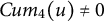 ,
${Cum}_4\left({e}_x\right)\ne 0$
,
${Cum}_4\left({e}_x\right)\ne 0$
 ,
${\unicode{x3b2}}_1\ne 0$
,
${\unicode{x3b2}}_1\ne 0$
 and
${\unicode{x3b2}}_2\ne 0$
and
${\unicode{x3b2}}_2\ne 0$
 :
:

Solving Equation (B2) for
$\eta$
 , the only two solutions are

Therefore, when
$\unicode{x3b7} =0$
 , it follows that
${\Delta }_1=0$
, it follows that
${\Delta }_1=0$
 and, assuming faithfulness holds (i.e.,
$\unicode{x3b7} \ne -\frac{\unicode{x3b2}_2}{\unicode{x3b2}_1}$
and, assuming faithfulness holds (i.e.,
$\unicode{x3b7} \ne -\frac{\unicode{x3b2}_2}{\unicode{x3b2}_1}$
 ), when
$\eta \ne 0$
), when
$\eta \ne 0$
 , then
${\Delta }_2\ne 0$
, then
${\Delta }_2\ne 0$
 .
.
Appendix C: A proof for Theorem 3
Theorem 3. Let
${\Delta }_3= Cum\left(x,x,y\right)\times Cum\left(x,y,y,y\right)- Cum\left(x,y,y\right)\times Cum\left(x,x,y,y\right)$
 . When no true causal effect from x to y exists (i.e.,
$\unicode{x3b7} =0$
. When no true causal effect from x to y exists (i.e.,
$\unicode{x3b7} =0$
 ), one obtains
${\Delta }_3=0$
), one obtains
${\Delta }_3=0$
 . When x truly causes y (
$\eta \ne 0$
. When x truly causes y (
$\eta \ne 0$
 ), with the faithfulness assumption that
$\unicode{x3b7} \ne -\frac{\unicode{x3b2}_2}{\unicode{x3b2}_1}$
), with the faithfulness assumption that
$\unicode{x3b7} \ne -\frac{\unicode{x3b2}_2}{\unicode{x3b2}_1}$
 and
$\unicode{x3b7} \ne -\frac{Cum_4(u){Cum}_3\left({e}_x\right){\unicode{x3b2}}_2}{Cum_4(u){Cum}_3\left({e}_x\right){\unicode{x3b2}}_1-{Cum}_3(u){Cum}_4\left({e}_x\right)}$
and
$\unicode{x3b7} \ne -\frac{Cum_4(u){Cum}_3\left({e}_x\right){\unicode{x3b2}}_2}{Cum_4(u){Cum}_3\left({e}_x\right){\unicode{x3b2}}_1-{Cum}_3(u){Cum}_4\left({e}_x\right)}$
 , one obtains
${\Delta }_3\ne 0$
, one obtains
${\Delta }_3\ne 0$
 .
.
Proof. Given Equations (8), (9), (11), and (12), we obtain

By setting
${\Delta }_1=0$
 and simplifying the result, we obtain the following cubic equation for
$\eta$
and simplifying the result, we obtain the following cubic equation for
$\eta$
 , assuming
${Cum}_4(u)\ne 0$
, assuming
${Cum}_4(u)\ne 0$
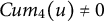 ,
${Cum}_4\left({e}_x\right)\ne 0$
,
${Cum}_4\left({e}_x\right)\ne 0$
 ,
${\unicode{x3b2}}_1\ne 0$
,
${\unicode{x3b2}}_1\ne 0$
 and
${\unicode{x3b2}}_2\ne 0$
and
${\unicode{x3b2}}_2\ne 0$
 :
:

Solving Equation (C2) for
$\unicode{x3b7}$
 , the only two solutions are

Therefore, when
$\unicode{x3b7} =0$
 , it follows that
${\Delta }_3=0$
, it follows that
${\Delta }_3=0$
 and, assuming faithfulness holds (i.e.,
$\unicode{x3b7} \ne -\frac{\unicode{x3b2}_2}{\unicode{x3b2}_1}$
and, assuming faithfulness holds (i.e.,
$\unicode{x3b7} \ne -\frac{\unicode{x3b2}_2}{\unicode{x3b2}_1}$
 and
$\unicode{x3b7} \ne -\frac{Cum_4(u){Cum}_3\left({e}_x\right){\unicode{x3b2}}_2}{Cum_4(u){Cum}_3\left({e}_x\right){\unicode{x3b2}}_1-{Cum}_3(u){Cum}_4\left({e}_x\right)}$
and
$\unicode{x3b7} \ne -\frac{Cum_4(u){Cum}_3\left({e}_x\right){\unicode{x3b2}}_2}{Cum_4(u){Cum}_3\left({e}_x\right){\unicode{x3b2}}_1-{Cum}_3(u){Cum}_4\left({e}_x\right)}$
 ), when
$\unicode{x3b7} \ne 0$
), when
$\unicode{x3b7} \ne 0$
 , then
${\Delta }_3\ne 0$
, then
${\Delta }_3\ne 0$
 .
.


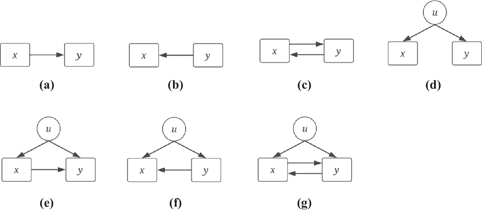
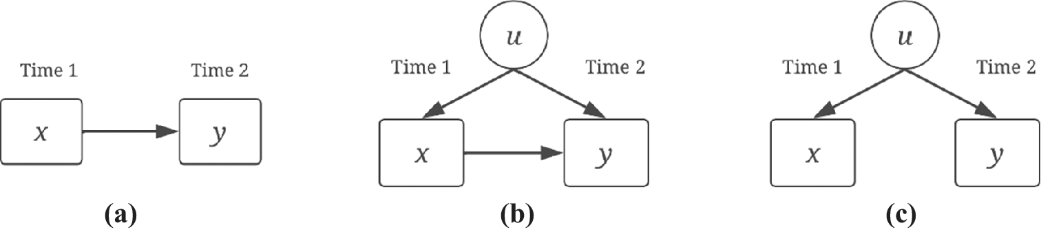
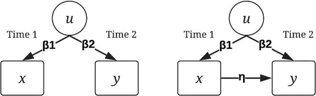
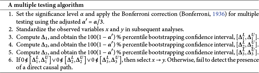


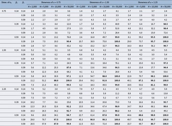

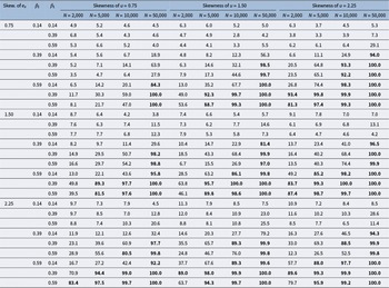

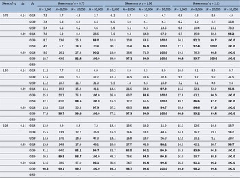


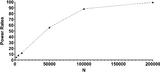




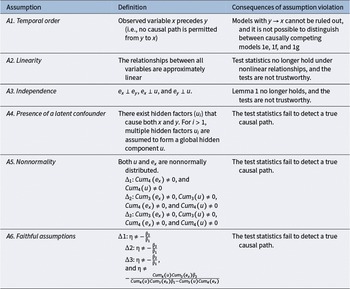


 Open access

