

Introduction
The undersides of floating ice shelves and sea ice in the Antarctic and Arctic are among the least accessible environments on Earth. Ice shelves several hundred metres thick, fed from parent ice sheets, float above submarine cavities that are up to 1 km deep and cover areas as large as about 500 000 km2 (e.g. Reference Jenkins and DoakeJenkins and Doake, 1991; Reference Mayer, Reeh, Jung-Rothenhäusler, Huybrechts and OerterMayer and others, 2000). The irregular calving of icebergs from marginal ice cliffs makes the close approach to both floating ice shelves and grounded tidewater-glacier margins hazardous. Sea ice, with ridged submarine keels that reach tens of metres deep, covers about 15 × 106 km2 of the Arctic Ocean and surrounds the Antarctic continent during winter (Reference Cavalieri, Parkinson and VinnikovCavalieri and others, 2003). The interactions between ice shelves, sea ice and the ocean are of considerable scientific interest, not least because the nature and rate of freezing and melting processes that take place are of wider significance to the global environmental system through their influence on, for example, water masses that flow equatorward as a driver of the thermohaline circulation of the oceans (e.g. Reference BroeckerBroecker, 1991).
Limitations of access have long precluded the thorough exploration and investigation of the cavities beneath ice shelves, where only a small number of drillholes have given access to the waters beneath (e.g. Reference NichollsNicholls, 1996; Reference Nicholls, Österhus, Makinson and JohnsonNicholls and others, 2001). Studies of the underwater morphology of sea ice have been restricted largely to the scientific utilization of submarines (e.g. Reference WadhamsWadhams, 1978, Reference Wadhams1988). The use of emerging technology in the form of unmanned underwater vehicles provides a method by which these very inaccessible and inhospitable parts of the global ocean and cryosphere can be investigated safely (Reference FrancoisFrancois, 1977; Reference Wadhams, Wilkinson and KaletzkyWadhams and others, 2004). Remotely operated vehicles (ROVs), tethered to a mother ship by an umbilical power and control cable, have been deployed to investigate tidewater-glacier and ice-shelf margins, but their range is restricted to hundreds or, at most, a few thousands of metres (e.g. Reference Dowdeswell and PowellDowdeswell and Powell, 1996; Reference Powell, Dawber, McInnes and PynePowell and others, 1996). However, the development of free-flying autonomous underwater vehicles (AUVs) provides a means to operate over ranges of tens to hundreds of kilometres and to depths below even the thickest floating ice shelves.
Here we describe briefly the specification of the Autosub2 AUV (Fig. 1), the scientific instrument packages it has deployed, and examples of applications to ice-shelf glaciology, sea-ice studies, oceanography and glacial geology in Antarctic and Arctic waters. Full details of the at-sea operations, together with an inventory of the scientific data, for the four cruises comprising the Autosub Under Ice programme are available on the website of the British Oceanographic Data Centre (BODC) at www.bodc.ac.uk/projects/uk/aui/cruise_programme.
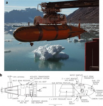
(a) The Autosub AUV being deployed in Courtauld Fjord, East Greenland, from RRS James Clark Ross. Autosub is 6.7 m long. Photograph by J.A. Dowdeswell. (b) The major systems of Autosub2 and the science sensors that were installed for the Autosub polar missions of 2003–05. The vehicle displaced 3.6 t and had a range of 400 km at 1.7 m s−1 with the payload of sensors shown.
The Autosub Autonomous Underwater Vehicle (AUV)
Design and power
Autosub2 is a 3600 kg, 6.7 m long AUV, with a 1600 m operating depth and range of 400 km at a forward speed of 1.7 m s−1. This vehicle is based on the earlier Autosub1, which had a 500 m depth limit (Reference MillardMillard and others, 1998). Autosub2 is referred to as Autosub through the remainder of this paper. For the polar science campaigns considered here, it was instrumented as illustrated in Figure 1b (Reference StevensonStevenson and others, 2003). Mechanically, the vehicle consisted of three sections. The front and rear sections were free-flooding, built around aluminium extrusion space-frames and covered with (replaceable) glass-fibre reinforced plastic (GFRP) panels. The central section comprised seven 3 m long carbon-fibre reinforced plastic (CFRP) pressure vessels, within a cylindrical matrix of syntactic foam – one central pressure vessel and the surrounding six at 60° intervals. These pressure vessels limited the vehicle operating depth to 1600 m at a safety factor of two. Four of the tubes housed the battery system of up to 5184 ‘D’ size primary manganese alkaline cells. With a total weight of 720 kg, these provided up to 60 kWh (220 MJ) of energy (depending upon usage rate and ambient temperature). Thermal insulation between the cells and the CFRP tubes enabled an internal temperature of >15°C to be maintained using the waste heat of the cells, despite external temperatures as low as −2°C (Reference Stevenson, Griffiths and WebbStevenson and others, 2002). The three other tubes housed electronics chassis for the control systems and sensors.
The rear section of Autosub housed essential subsystems (navigation, control actuation and propulsion) and scientific sensors (e.g. digital camera, upward-looking 300 kHz Teledyne RDI acoustic Doppler current profiler (ADCP), 200 kHz multibeam receiver). A single brushless direct-drive (no gearbox) direct-current motor and five-bladed propeller gave the vehicle a speed of 1–2 m s−1. A rear-mounted rudder and stern-plane controlled vehicle yaw, pitch and depth.
The free-flooding front section of Autosub housed other essential vehicle subsystems (forward-looking collision sensor, emergency abort, the homing system, Argos transmitters and flashing lights for relocation) as well as science sensors (e.g. twin Seabird 911 conductivity–temperature– depth (CTD) instruments, multibeam transmitter, EdgeTech sub-bottom profiler, Envirotech AquaLab water-sampling system). Payload restrictions meant that, on any given dive, it was possible to deploy in the front and rear sections of Autosub only a subset of the instruments actually available.
The control and data system for Autosub was based upon a distributed and networked control architecture (Reference McPhail and PebodyMcPhail and Pebody, 1998). With such architecture it is relatively straightforward to add new sensors onto the vehicle without affecting the safe operation of the control system.
Navigation and control
The rationale for a highly accurate navigation system was that when executing under-ice missions the vehicle would be required to travel 100 km or more without the possibility of global positioning system (GPS) position fixes or tracking from the mother ship. Furthermore, it would need to navigate its way back to a relatively small hole in the ice or to a polynya. The two primary sensors for navigation were a 150 kHz Teledyne RDI ADCP and Ixsea-Oceano PHINS fibre-optic gyro-based inertial navigation system (INS). To obtain the best possible navigational accuracy (errors of <0.2% of distance travelled were typically achieved, even at 80° N), the downward-looking ADCP must be able to track the seabed. The missions under the ice shelf needed as great a bottom-tracking range as possible. This meant the use of a relatively low-frequency (150 kHz) ADCP (with a bottom track range of 500 m) rather than higher-frequency versions typically fitted to AUVs. Both the INS and the 150 kHz ADCP were housed within a single pressure case so that the vital mechanical alignment between the ADCP and INS could be maintained accurately between missions. The navigation system was also able to utilize the velocity-tracking data from the upward-looking 300 kHz ADCP. This would be used when the Autosub was flying within a cavity under an ice shelf, close enough to obtain useful velocity-tracking data from the underside of the essentially stationary ice shelf (at <150 m range), but too far from the seabed to use the (preferred) seabed-tracking mode.
Collision-avoidance and emergency beacon systems
In polar waters, uncharted bathymetry, icebergs, sea-ice pressure ridges and the undersides of ice shelves with their unknown topography are all possible collision risks. This led to the development of a strategy, system and algorithms for collision avoidance specifically designed for polar operations. The system relied upon the use of sensors and data already available on the vehicle, these being:
Paroscientific Digiquartz pressure sensor
Four upward-looking ADCP beam ranges
Four downward-looking ADCP beam ranges
Forward-looking echo sounder (Simrad Mesotech 120 kHz)
The approach was to keep the hardware and software as simple as possible, triggering one straightforward, yet effective, behaviour upon detecting that a collision was imminent.
Collision-avoidance mode was entered if:
the forward-looking echo sounder detected an object continuously closing on the vehicle, and at a range <100 m, or
there was <50 m depth of water in which the vehicle could operate.
Once collision-avoidance mode was triggered, the vehicle was programmed to backtrack for 1 km along its previous course. It then returned along its original route, but with an offset of up to 500 m either side of its pre-planned track. Simultaneously, the AUV adjusted its depth safety limits, increasing the margin of safety in the vertical plane. If an imminent collision was detected again, the vehicle repeated the collision-avoidance manoeuvre, but with a new randomly chosen track offset. Once clear of the obstacle, the original course and safety limits were restored. An example of the operation of the collision-avoidance algorithm, allowing Autosub to circumvent an obstructing object, is shown in Figure 2.
Plan view of collision-avoidance behaviour, triggered by detection of a 30 m deep iceberg keel ahead on mission 365 off northeast Greenland (Reference Wadhams, Wilkinson and McPhailWadhams and others, 2006). It took three attempts for Autosub to avoid the hazard and continue eastwards on its programmed course. Axes are in decimal degrees north and west.

If the Autosub systems detected a critical failure, or if there was a catastrophic power loss during the mission, an emergency acoustic beacon would be dropped on a 15 m cable, transmitting a 4.5 kHz chirp once per minute. The beacon would be heard on the ship using a vertical-array receiver deployed to a depth of up to 100 m. By timing the arrival of the received signal at each of three or more ship’s positions, it would be possible to triangulate Autosub’s position up to a range of 30 km.
Deployment and recovery in ice
Whereas many handling problems of AUVs in the open ocean are a result of high sea states, in polar waters the main difficulties arise from fast-changing ice conditions. During the first Autosub campaign in the Antarctic, the vehicle was launched and recovered in areas that were virtually clear of ice (Reference BrierleyBrierley and others, 2002). However, sea-ice cover remained a hazard if the wind was blowing the ice out to sea. In such circumstances, the launch and recovery position could be tens of kilometres away from the area of interest and a large proportion of battery energy was expended simply getting Autosub to the ice edge.
For subsequent campaigns, a sink-weight release system was developed, allowing the vehicle to be launched in any ice-free patch of water. This avoided the need for a large open-water area to allow Autosub to dive from the surface at a shallow inclination. At a predetermined depth, usually 15–20 m, a 20 kg weight slung beneath the nose would release and the propulsion motor would start. The whole autonomous mission from that point would be carried out submerged. A disposable passive hydrostatic safety release was fitted between the weight and the programmable release to ensure that the weight fell away in the event of the programmable release failing. The sink-weight system greatly enhanced the effectiveness of under-ice work by facilitating deployment close to the ice edge.
Water-density gradients
Autosub is ballasted to be 8–12 kg positively buoyant in water and final ballast adjustments were usually made on the working site after taking water-density measurements. When working close to an East Greenland tidewater glacier, a density difference of 4 kg m−3 between the surface and 6 m was present. This density difference produced a 10 kg increase in buoyancy for the vehicle at its working depth and was on the verge of making the vehicle unable to control its depth. The solution adopted to cope with these density variations was to fit ‘winglets’ (160 mm half-span by 254 mm chord) slightly aft of the centre of gravity of the vehicle to produce additional downward force while moving. These proved effective and had the added benefit of reducing body pitch angle.
Surfacing in ice and homing system
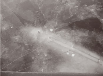
Autosub had two Argos satellite transmitter antennae and one WiFi Ethernet radio antenna mounted externally. These were vulnerable and could be damaged by the ice before the vehicle had been located visually, potentially resulting in vehicle loss simply because it could not be located. Even when ice cover was very light, it was clear that antennae could be broken easily and the vehicle could become ice-covered (Fig. 3). Autosub is particularly dependent on the Argos transmissions for location at the end of missions and a GFRP tube was made to fit over the forward antenna to give some protection against ice damage. The experience highlighted the need to control the final stages of the end of the mission remotely rather than trying to second-guess ice conditions at the mission programming stage.
Autosub surfacing in light sea-ice cover. Note the possibility of damage to antennae protruding from the vehicle.
On occasions, due to drifting sea ice, it was not possible at the time of launch to be certain that the recovery position would be clear of ice. Further, there was a need to be able to cope with situations in which the mother ship could not reach the intended recovery position, or when unexpected navigation system drift, or some other failure, could leave the AUV still operating but a long way off the intended recovery position.
To deal with these eventualities a homing system was developed, able to guide Autosub back towards the mother ship at ranges of up to 15 km. The shipboard homing beacon transmits regularly spaced swept frequencies (chirps), centred at 4.504 kHz. On the vehicle were three spherical hydrophones, which, together with the three-channel correlation receiver, allowed the direction of arrival of the homing signal to be determined. Once the system had detected four consecutive transmissions with the correct temporal spacing, the AUV entered homing mode and headed towards the source of the signal. This system was used successfully during the northeast Greenland campaign of 2004, where on mission 365 the intended recovery position had been covered by sea ice as a result of changing wind conditions.
Instrumentation for the Autosub AUV
Geophysical instruments
A swath-bathymetry system or multibeam echo sounder was included in the Autosub instrument package to measure the geometry of both the underside of ice shelves and sea ice, together with sea-floor morphology. The system could be configured to operate in upward- or downward-looking mode for glaciological and glacial–geological applications, respectively. A Kongsberg Simrad EM-2000 swathbathymetry system was used. It operates at a frequency of 200 kHz, has 111 individual beams, an angular coverage of over 120°, and a swath width of up to 300 m (depending on distance from target). Quantitative data on elevation can be gridded at a horizontal resolution of 1 m. Root-mean square (rms) errors of better than 10 cm can be achieved in the vertical. A swath-bathymetry system was preferred to a conventional marine side-scan sonar instrument because it provides quantitative three-dimensional (3-D) morphological data of high absolute accuracy, rather than imaging changes in backscatter that relate to both geometry and surface properties.
An EdgeTech chirp penetration echo sounder was also mounted on Autosub to investigate the acoustic stratigraphy of the sea floor. The profiler operates at 2–16 kHz and penetrates through up to several tens of metres of sediment, depending on grain-size, density and pore-water characteristics with a vertical resolution of 6–10 cm. Both geophysical instruments log data to internal hard drives for the duration of each Autosub mission.
Oceanographic instruments
Autosub was equipped with a Seabird 911 plus CTD system, which included two pairs of temperature and conductivity sensors. A dissolved oxygen sensor was also attached, although for accurate oxygen measurements this needed to be calibrated against laboratory measurements on concurrent water samples. The Seabird conductivity and temperature sensors were, in general, remarkably stable so that, with two pairs and regular calibration, high accuracy measurements were possible. The specified drift rate for the temperature and conductivity sensors was 0.002°C a−1 and 0.0024 siemens m−1 a−1 (0.0023 Ω m−1 a−1), respectively. The two essentially independent sensor pairs provided a check on the data quality, and we have typically found the pairs differed by no more than 0.001’C in temperature and no more than 0.002 in derived salinity. The deployment of a shipboard CTD before or after an Autosub mission provided a cross-check that the Autosub CTD sensors were making reasonable measurements. The Autosub CTD data were processed using the software provided by the manufacturer, following the standard processing pathway set out in the user manual for the software. This included calculating salinity and other derived variables.
Upward- and downward-looking Teledyne RDI ADCPs were fitted, which were used both for navigation and scientific measurements. The downward-looking 150 kHz instrument typically returned current measurements up to 150–200 m below Autosub. The upward-looking 300 kHz instrument typically provided more limited range, up to about 100 m above Autosub. The Autosub ADCP data were processed using a system of dedicated MATLABTM scripts.
Photographic instruments
Autosub was equipped with a Starlight SXV-H9, which is a black-and-white charge-coupled device (CCD) imager, to obtain images of the sea floor and the marine benthos close to and beneath floating ice. The imager was selected for its high sensitivity (particularly in the important blue part of the spectrum), low readout noise (about 20 photons rms equivalent) and high dynamic range. An integral data logger records the images on hard disk, which can be accessed via the Autosub radio network. The camera is installed in the tail section of Autosub, and a Minolta zoom flash is installed within a pressure case at the nose of Autosub. The image sensor has an array of 1040 × 1392 of 6 μm square pixels, making an imager size of 6.24 × 8.35 mm. With an air–water magnification factor of 1.4, this equates to an image diagonal of 2.2 m at a flying altitude of 10 m. The camera data are stored in a raw 16-bit binary format.
Water-sampling instruments
Autosub carried a compact water sampler to allow the measurement of a wide range of water properties. The sampler was an Envirotech AquaLab, which consists of a mechanical syringe that draws water into one of 49 EVA plastic sample bags by means of a rotary valve (Fig. 4). Samples are suitable for most tracer and nutrient studies, but not for the measurement of trace gases, due to the gaspermeable nature of the EVA bags used.
The AquaLab water sampler located in the nose of the Autosub vehicle. Individual water-sample bags are visible. Photograph by P. Dodd.

Before deployment, sample bags must be filled with a small volume of ‘prime’ fluid so that hydrostatic forces do not crush connecting parts. Ordinarily, this fluid is flushed out of each bag in situ before a sample is collected. However, this time-consuming procedure can be avoided if bags are filled with a prime fluid in which the properties of interest are known and later accounted for (Reference Dodd, Price, Heywood and PebodyDodd and others, 2006). This approach allows a 200 mL sample to be collected in 8–10 min during which Autosub would travel just under 1 km at a cruising speed of 1.6 m s−1. Samples of any size can be collected, but multiple syringe strokes are required to collect samples larger than 200 mL.
The water sampler is capable of operating in an autonomous mode, in which samples are collected at predetermined times, or it can be triggered by Autosub to collect samples at specific locations. It is also possible for Autosub to circle while a sample is collected and continue only when the sampler reports that sampling is complete. To date, the sampler has provided samples for oxygen-isotope ratio and barium concentration measurements (Reference Dodd, Price, Heywood and PebodyDodd and others, 2006).
AUV Observations of Ice, Ocean and Sea Floor: Some Examples
Ice shelves: the underside of an Antarctic ice shelf
Traditional methods for determining the topography of an ice-shelf base have used either downward-looking radar from above the upper surface of the ice shelf, generally from an aircraft platform, or the inversion of elevation data of the upper surface under the assumption that the ice column floats in hydrostatic equilibrium (Reference Bamber and BentleyBamber and Bentley, 1994; Reference Dowdeswell and BamberDowdeswell and Bamber, 2007). Both techniques have their advantages: inversion of (typically) satellite-derived surface elevations gives very good spatial coverage at horizontal scales somewhat longer than the ice is thick; downward-looking radar gives a detailed view at horizontal scales determined by the ice thickness and the wavelength of the radar waves in ice. Reliance on the results from these techniques has reinforced the notion that the base of ice shelves is generally rather smooth, and can be regarded as having a drag coefficient at the ice–water interface similar to that of the sea floor. Neither technique, however, is able to reveal basal topography at the scales important to the friction exerted on water flow beneath the ice shelf, a parameter important to the realistic modelling of flow beneath the ice shelf.
Autosub’s mission 382, beneath Fimbul Ice Shelf, East Antarctica, yielded the first acoustic image of the base of an ice shelf (Fig. 5). The upward-looking multibeam echo sounder gave a 150 m wide image of the base of this ice shelf along 18 km of the mission track. For most of the swath, the vehicle was 90 m below the ice base. The draft of the ice shelf, as seen by the multibeam system, is shown in Figure 5a. The breadth of the swath is an indication of the specularity of the ice base, with a broader swath indicative of a rougher base. Much of the swath suggests an almost specular reflection, consistent with the generally held view that the base of an ice shelf is rather smooth (Reference Holland and FelthamHolland and Feltham, 2006). A substantial fraction, however, is very rough. Figure 5b shows a 3-D visualization of a rough portion of the swath, from 18.9 to 21.5 km along track, illustrating that the basal ice-shelf topography is quite chaotic at horizontal length scales of 10 m or less, with vertical scales similarly of the order of 10 m. In reality, the image in Figure 5 is a substantially smoothed visualization, as the extreme nature of the terrain caused excessive shadowing which has been filled-in in a smooth manner.
(a) Multibeam data from mission 382 beneath Fimbul Ice Shelf, East Antarctica, showing ice-shelf draft (m), the track starting beneath the ice shelf (0 km) and ending at the ice front (26 km). (b) 3-D rendering of swath-bathymetric data, showing a portion of the ice base below a flow trace at 20 km, including the smooth base either side of the feature (from Reference NichollsNicholls and others, 2006).

The rough portions of the swath data correspond on the ice-shelf surface to flow traces. These flow traces are linear features visible from aerial or satellite imagery (Reference Fahnestock, Scambos, Bindschadler and KvaranFahnestock and others, 2000) that are often initiated at glacial features, such as shear margins, or associated with regions of fast flow. Flow traces are ubiquitous on ice shelves and, if they are generally underlain by an ice base with such dramatic topography, it is clear that the frictional drag imposed on the ocean circulation beneath the ice shelf needs to be reassessed (Reference NichollsNicholls and others, 2006).
Sea ice: a three-dimensional view
In August 2004 the Autosub AUV, in operations off northeast Greenland, obtained the first successful multibeam sonar measurements under sea ice, giving a quantitative map of the 3-D nature of the under-ice surface (Reference Wadhams, Wilkinson and McPhailWadhams and others, 2006). The vehicle, operating from RRS James Clark Ross, obtained more than 450 track-km of under-ice multi-beam sonar data using the Kongsberg EM-2000 system. Figure 6 shows examples of imagery from first- and multiyear ice, including young ridges, old hummocks and undeformed melting ice. The imagery was obtained from mission 365 on 21–22 August 2004, which headed west across the shallow Belgica Bank at 79°30′ N under partially grounded multi-year ice, then penetrated further over the 500 m deep Norske Trough, occupied mainly by undeformed first-year fast ice. Each of the displayed images is a perspective view of the underside of the ice, obtained with the AUV at 40 m depth, with scenes shown as if illuminated by a sun of elevation 20°.
Examples of EM-2000 swath-bathymetric images of the under surface of sea ice offshore of northeast Greenland. The perspective views are illuminated by a sun elevation of 20°. (a) An embedded multi-year floe with a 33 m deep sea-ice ridge. The floe is surrounded by undeformed shorefast sea ice. (b) A multi-year ridged floe of draft 3–5 m, embedded in undeformed shorefast ice of draft 1.8 m. Fast ice shows a pattern of depressions due to mirroring of surface melt pools. The floe contains a pressure ridge of maximum draft 11 m, which has partly disintegrated into individual ice blocks of diameter 5–20 m (from Reference Wadhams, Wilkinson and McPhailWadhams and others, 2006).

Two swath-bathymetric images of the underside of Arctic sea ice are shown. Figure 6a illustrates the deepest ridge encountered during mission 365, which has a 33 m draft. This ridge is embedded in a larger multi-year floe (from ∼3200 to 3800 m) that probably drifted out from the Arctic Ocean the previous summer. The undeformed ice surrounding this floe is 1.75 m in draft and is almost certainly first-year ice. Since the individual ice blocks that make up ridges are quite small, the ridge is a relatively uniform triangle in cross-section, representing the angle of repose of a pile of buoyant ice. A number of thinner floes, 10–15 m in draft, are also visible in the image.
Figure 6b shows an old multi-year ridged floe of thickness 3–5 m which is embedded in younger fast ice of draft 1.8 m. The edges of the floe are sharp and linear as would occur with a fracture that occurred just before embedding. The ridge which occupies half of the floe has maximum draft of 11 m and contains separate ice blocks of typical diameters 5–20 m. In the ice surrounding the embedded floe a number of small floes, with drafts of about 10 m, are present. The faint pattern of depressions in the underside of the thinner ice occurs because of the presence of meltwater pools on the upper surface. These pools preferentially absorb incoming radiation, giving a heat flux that enhances bottom melt and generates a bottom depression which mirrors the position of each pool on the top side (Wadhams and Martin, 1990; Reference WadhamsWadhams, 2000).
Oceanography: the nature of a water-filled cavity beneath an ice shelf
The majority of Antarctic Bottom Water (AABW) is thought to have its origins in processes that take place over the Antarctic continental shelf. These processes therefore reflect the importance of AABW as a key component in the global thermohaline circulation. As a consequence, interactions between the Southern Ocean and Antarctic ice shelves, which cover 40% of the Antarctic continental shelf, are also important. Historically, exploration of the processes beneath ice shelves has been restricted to what can be achieved by drilling access holes and deploying oceanographic instrumentation into the water column beneath. The process of making access holes is demanding logistically, and a rather small number of holes can be made in any given Antarctic field season. In fact, fewer than 30 access points have been made across all ice shelves in Antarctica. Clearly AUVs offer an opportunity to improve substantially our ability to obtain data from this unique environment.
During mission 382 to the cavity beneath Fimbul Ice Shelf, Autosub executed a simple in–out track with a total track length of 60 km, 53 km of which was beneath the ice shelf. The in-going track was at an elevation above the seabed of 150 m. The vehicle then turned on a reciprocal track, ascending to an elevation of 400 m. The fact that the seabed shallows towards the ice front, combined with an overriding instruction to maintain a minimum headroom from the ice base of 90 m, meant that Autosub was terrain-following off the base of the ice shelf for much of the return track.
The temperature, salinity and current-speed data obtained from the primary oceanographic instruments during the mission are shown in Figure 7. These data exhibit a wealth of detail, and are discussed by Reference NichollsNicholls and others (2006) in the context of data obtained from the front of the ice shelf using the ship. The principal conclusion of Reference NichollsNicholls and others (2006) was that, as the properties of some of the waters observed within the cavity did not relate to the waters observed along the front of Fimbul Ice Shelf at the time of the mission, the cavity must be flushed episodically by relatively warm water that crosses the continental-shelf break from the north, possibly during the winter.
Oceanographic data from mission 382 obtained beneath Fimbul Ice Shelf, Antarctica. (a) Mission trajectory (red and blue lines indicate the outward and return Autosub legs, respectively). The vertical dashed line at 26.5 km gives the position of the ice front, referenced to the turning point in the mission; the horizontal dashed line at 570 m depth shows the depth of a nearby sill at the continental-shelf break. Also shown are the ADCP data illustrating the dramatically reduced range beneath the ice shelf that implies a dearth of appropriately sized scatterers in the water column. The upward-looking instrument operated at 300 kHz and the downward-looking instrument at 150 kHz. The data are for the north– south velocity component (positive northward, approximately perpendicular to the ice front), which have been averaged using a horizontal window 100 m wide. The inset shows the ADCP data in the vicinity of the ice front for the outward leg. (b) Vertically averaged ADCP currents after subtraction of the modelled tide. (c) Salinity (bold) and potential temperature (θ). The thin green near-horizontal dashed line is the freezing point of the water at surface pressure for salinities measured on the outward journey (from Reference NichollsNicholls and others, 2006).
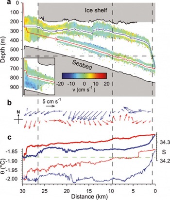
An intriguing dataset acquired by the Autosub ADCPs is shown in Figure 7a. The effective range of an ADCP in large part depends on the number and type of scatterers in the water column, and their size with respect to the wavelengths in the acoustic pulse. With a wavelength of 10 mm, the 150 kHz downward-looking instrument generally has a greater range than its 300 kHz upward-looking counterpart. This can be seen outside the cavity on the left side of Figure 7a. Once Autosub has passed beyond one or two tidal excursions into the cavity (a distance of about 3 km), the range of both instruments decreases markedly and the performance of the 300 kHz ADCP overtakes that of the 150 kHz instrument. The performance of the ADCPs indicates a different biological assemblage beneath the ice shelf, implying a reduction in the volume density of biological material and a shift towards smaller-sized scatterers. The rapid fall-off with distance into the cavity of scatterer volume density also suggests that this is an area of outflow.
Although investigation of the ocean processes within cavities beneath ice shelves will always require moored instruments capable of collecting data over periods of months or years, Autosub’s ability as a platform that can use sophisticated oceanographic instrumentation to generate spatially extensive datasets has given us a unique view of one of the least accessible parts of the world’s oceans.
Autosub was lost under the Fimbul Ice Shelf on mission 383, the one following that described above. Its low-frequency acoustic beacon signalled that an abort had been triggered and that the vehicle was stuck at a position approximately 17 km from the ice front. A full investigation (Reference StruttStrutt, 2006) concluded that either an open-circuit or network failure was the most likely cause of an abort or loss of power. This was the only time the vehicle deployed its long-range acoustic beacon.
Oceanography: fjord circulation and meltwater flux
The circulation and mixing processes of water masses within fjords can be complex, so one advantage of a rapid and continuous surveying device such as Autosub is to enable a more synoptic survey than is achievable with a ship. Typically, saline ocean water enters a fjord at mid-depth above the sill, and fresh meltwater from the surrounding glaciers or rivers exits the fjord as a surface layer (Reference Syvitski, Burrell and SkeiSyvitski and others, 1987). The deep waters within the fjord are renewed only sporadically. However, this steady-state simple picture can be complicated by the presence of tides, cross-fjord flows, sea ice entering and/or leaving the fjord, and the flows induced by inertial oscillations following storms. The net exchange of fresh water between a fjord and the continental-shelf environment is of importance in determining, for example, the influence of meltwater from the Greenland ice sheet on the formation of dense water masses in the seas surrounding Greenland.
The detailed current-velocity structure revealed by the Autosub ADCPs at the mouth of Kangerdlussuaq Fjord on the east coast of Greenland is shown in Figure 8. In the 6 hours of this survey, three passes across the fjord were made at depths of 70, 190 and 400 m. The upward- and downward-looking ADCPs are very consistent between adjacent passes some 4 hours apart, implying that tidal (or other temporally varying) flows are not dominant here. However, the velocity structure is very different from the simple three-layer flow suggested above. The primary inflows are on the southwest side of the mouth at 300–400 m and in the upper 100 m. The primary outflow is at about 200–350 m on the northwest side of the fjord mouth, implying a clockwise circulation of open ocean water in the bay at the mouth of the fjord. There is a suggestion that the water in the top 10 m may be a thin layer of ice melt leaving the fjord. Thus, Autosub has revealed, in unprecedented detail, a snapshot of the complex exchanges between an Arctic fjord environment and the adjacent continental shelf.
Cross-section of the current velocity (colour scale in m s−1) into and out of the mouth of Kangerdlussuaq Fjord, East Greenland, acquired from the upward- and downward-looking ADCPs mounted on Autosub. The Autosub navigated horizontal paths at 70, 190 and 400 m (marked as black lines), descending or rising in between, taking 6 hours to complete the survey. Positive values denote water flowing into the fjord; negative values indicate water flowing out of the fjord. Southwest is to the left and northeast to the right.

Oceanography: attenuation of waves by sea ice
A serendipitous result for the behaviour of waves propagating in sea ice was obtained from the upward-looking ADCP surface track velocity recorded on Autosub. Because the surface track ping has longer range than the profile ping, the velocity of sea ice relative to Autosub could be measured during runs as deep as 200 m. This was the first use of an AUV to measure directional and scalar wave properties during surface wave propagation through sea ice (Reference Hayes and JenkinsHayes and others, 2007). Since ice-edge detection was also possible from the surface track ping (verified by ship observations), dependence of the above wave properties on distance from the edge of the marginal ice zone could be examined.
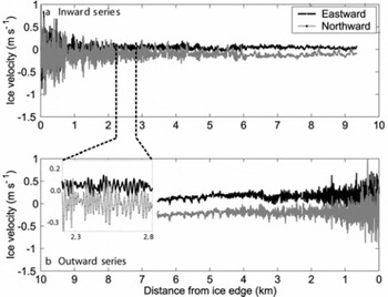
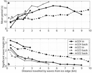
As an example, during mission 324 on 25 March 2003 in the marginal ice zone of the Bellingshausen Sea, Antarctica, the horizontal velocity of the ice was oscillating. The magnitude of this oscillation also decayed with distance from the ice edge both on the inward and outward segments (Fig. 9a). In the observed regime of small ice floes (<20 m) and long wavelength (100–350 m), the floes nearly follow the circular path of a point on the water surface. Therefore, the surface track velocity is regarded as a measurement of surface wave orbital velocity, superimposed on mean ice velocity (southeastward in the case of mission 324). The series is divided into a number of blocks (Fig. 9b) to analyze the surface velocity. The directional and scalar wave spectra are calculated for each segment, so any trend in significant wave height, mean and peak wave periods, as well as any change in the energy, wave direction or spread of various frequency components can be detected (Fig. 10). The character of waves propagating through sea ice that was observed using Autosub agrees with most of the previous observational (Reference Wadhams, Squire, Ewing and PascalWadhams and others, 1986, Reference Wadhams, Squire, Goodman, Cowan and Moore1988; Reference Liu, Holt and VachonLiu and others, 1991) and numerical (Reference Meylan, Squire and FoxMeylan and others, 1997) experiments.
Sea-ice velocity from Autosub mission 324. The upward-looking ADCP measured the surface track velocity upon (a) entering the ice pack at 90 m and (b) exiting the ice pack at 90 m. The magnified inset shows a typical segment analyzed here. Note the strong periodicity in both components, as well as mean current towards the southeast (modified from Reference Hayes and JenkinsHayes and others, 2007).
(a) Mean wave period and (b) significant wave height for Autosub missions 322–324. The label ‘in’ refers to the series collected upon entering the ice pack, while ‘back’ refers to the return series. Period and wave height are derived from the one-dimensional wave spectrum of 512 s blocks (with the exception of the return trip in mission 323 in which 256 s blocks were analyzed).
Glacial geology: submarine glacial landforms and acoustic stratigraphy
The morphology and stratigraphy of the sea floor provide important evidence for the reconstruction of the dimensions and flow of former ice sheets (e.g. Reference AndersonAnderson, 1999). Where ice flows across a sedimentary bed, landforms diagnostic of ice-flow direction and dynamics are produced. These land-forms, which are often streamlined, are preserved under water as ice retreats across continental shelves and fjords during interglacial and interstadial periods (e.g. Reference Anderson, Shipp, Lowe, Wellner and MosolaAnderson and others, 2002; Reference Ottesen, Dowdeswell and RiseOttesen and others, 2005; Reference Evans, Dowdeswell, Cofaigh, Benham and AndersonEvans and others, 2006). Characteristic assemblages of these submarine landforms are indicators of, for example, ice-stream flow, past glacier-surge activity and former grounding lines (e.g. Reference Powell, Dawber, McInnes and PynePowell and others, 1996; Reference Canals, Urgeles and CalafatCanals and others, 2000; Reference Ó Cofaigh, Pudsey, Dowdeswell and MorrisÓ Cofaigh and others, 2002; Reference Ottesen and DowdeswellOttesen and Dowdeswell, 2006).
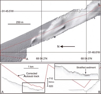
The swath-bathymetry system on Autosub, when mounted in downward- looking mode, produces data that yield high-resolution digital-terrain models and 3-D images of the sea floor. Figure 11 shows the floor of an East Greenland fjord, where the fast-flowing Kangerdlussuaq Glacier, one of the major outlet glaciers of the Greenland ice sheet (Reference Rignot and KanagaratnamRignot and Kanagaratnam, 2006), has produced streamlined sedimentary bedforms which are preserved in several hundred metres of water after ice retreat from its position at the Last Glacial Maximum (Reference Syvitski, Andrews and DowdeswellSyvitski and others, 1996). Shallow acoustic stratigraphy provides further information on the structure of the upper few metres to tens of metres of sediment. In the example shown in Figure 11b, the acoustic profiler on Autosub penetrates the fine-grained and acoustically laminated sediments in the deepest part of Kangerdlussuaq Fjord, with less transparent and probably coarser-grained sediments characteristic of glacial diamicts or tills to either side. Autosub, which has been deployed close to the calving tidewater margins of Courtauld Glacier, East Greenland (Fig. 1a), can be used to image areas of the sea floor in previously inaccessible locations near calving ice cliffs and beneath ice shelves.
Multibeam echo-sounder image of the glacially streamlined sea floor of Kangerdlussuaq Fjord, acquired from a 200 kHz swathbathymetry system mounted on Autosub. The swath width is approximately 200 m. Water depth is 710–840 m. The swathbathymetry data are gridded at a resolution of 1 m in the horizontal. The lower panels show acoustically stratified sediments on the fjord floor, acquired from the chirp 2–16 kHz sub-bottom profiler on Autosub. The acoustic profile is located in the multibeam image.
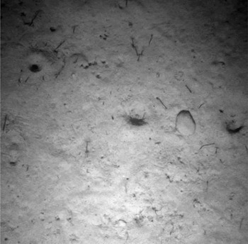
In addition to geophysical instruments, the digital camera equipment on Autosub provides detailed information on the form and composition of the sea floor and the marine biota that inhabit it. Figure 12 shows an example of a sea-floor photograph acquired by Autosub in Kangerdlussuaq Fjord. Both individual dropstones, released by iceberg melting, and bottom-dwelling marine organisms are shown. The presence of deposit-feeding species is indicated by faunal traces on the sediment surface. Evidence of disturbance to the seabed and fauna from iceberg-keel ploughing was also observed in photographs of the sea floor at water depths less than about 500 m, reducing faunal density and diversity as well as producing a sedimentologically heterogeneous environment.
Example photograph from Autosub mission 377, showing the floor of outer Kangerdlussuaq Fjord (imaged from an altitude of 9 m at a depth of 564 m). One cobble-sized iceberg-rafted drop-stone, three large burrows and numerous tubeworms are visible. The photograph is about 1 m across.
Conclusions
The Autosub AUV provided a platform for the deployment of a number of geophysical and oceanographic instruments in hazardous polar environments that ships and other manned vehicles cannot access.
Ice-covered environments investigated using Autosub include a cavity beneath the Fimbul Ice Shelf, and the relatively shallow and poorly charted waters beneath sea ice on the East Greenland continental shelf.
The multibeam echo sounder of Autosub has imaged the underside of an ice shelf for the first time, showing that some areas are very rough, with implications for the modelling of water flow and melt rates. The underside of sea ice has also been imaged in detail and quantitative shape parameters extracted. Swath images and bottom photographs of the glacial geology and marine biota close to the margins of Arctic tidewater glaciers have also been obtained.
Oceanographic data such as salinity, temperature and water velocity have been derived continuously during Auto-sub missions beneath floating Arctic and Antarctic ice, providing observations with a very dense spatial coverage in environments where previously few or no data have been available.
The Autosub3 vehicle, successor to the lost Autosub2, and AUV technology in general, is likely to be used increasingly in hazardous polar marine environments for the collection of detailed geophysical and oceanographic data close to and beneath floating ice. These data, in turn, are important in the calibration and testing of numerical models relating to ice-sheet interactions with the polar waters.
Not all of the scenarios for AUV operations in polar seas have yet been achieved in practice, although many have been described and discussed by scientists and engineers (Reference Griffiths and CollinsGriffiths and Collins, 2007; Reference Collins and GriffithsCollins and Griffiths, 2008). In August 2007, the first AUV campaign took place to search for, and then examine, hydrothermal sites at the slow-spreading Gakkel Ridge in the Arctic Ocean, an area of extensive multi-year pack ice (Reference Reves-SohnReves-Sohn and others, 2007). Other plans include multidisciplinary studies beneath the Ross Ice Shelf, Antarctica, and surveys of Southern Ocean krill populations in winter.
Acknowledgements
This work was supported by the Autosub Under Ice Thematic Programme of the UK Natural Environment Research Council (Programme Chair, S. Ackley; Programme Manager, K. Collins). We are grateful to the Autosub Technical Team and the officers and crew of RRS James Clark Ross for their invaluable contributions on four Autosub cruises.


