


Impact statement
The present work establishes a reliable and efficient framework for the buckling design of thin-walled truncated conical shells by alleviating the long-standing over-conservatism inherent in code-based KDF provisions. Through the application of various data-driven ML models, including the newly proposed hybrid (GPR + XGB) model, the study demonstrates that KDFs can be predicted with higher accuracy and substantially with reduced conservatism while remaining in close agreement with experimental evidence. These outcomes support a more rational and economical design philosophy, with the potential for meaningful material savings and improved structural performance in aerospace, marine, and other engineering applications. Finally, the proposed extension to physics-informed neural networks (PINNs) provides a promising direction for enhancing prediction robustness in data-limited scenarios by tightly coupling mechanics-based principles with advanced ML techniques.
1. Introduction
Thin-walled conical shells are extensively used in aeronautical, structural, offshore and pipeline engineering applications and are frequently subjected to axial compressive loads that can trigger buckling. For varying geometry of the shell, a series of experimental data were presented by Seide (Reference Seide1961, Reference Seide1962) and Weingarten et al. (Reference Weingarten, Morgan and Seide1965) for axially compressed isotropic conical shells. However, remarkable discrepancies between the theoretical and the experimental critical loads have been observed. Multiple studies have been conducted to investigate such discrepancies. Geometric imperfections, pre-buckling nonlinearity, modal multiplicity, erosion of membrane energy are primarily attributed to such reduction in the critical load (Arbocz, Reference Arbocz1968; Friedrich and Schroder, Reference Friedrich and Schroder2016). Therefore, the theoretical buckling load is multiplied with a conservative KDF to obtain the actual buckling load. A uniform KDF value of 0.33 is recommended by NASA SP-8019 (Weingarten and Seide, Reference Weingarten and Seide1968) irrespective of the cone geometry. However, such estimate of KDF is highly conservative in nature. An equivalent cylindrical approach may be adopted for the semi-vertex angle β ≤ 100 according to NASA: SP-8007 (Peterson et al., Reference Peterson, Seide and Weingarten1968). Rotter (Reference Rotter, Teng and Rotter2004, Reference Rotter2008, Reference Rotter2017) also established a suitable design criterion for conical shells which is also adopted by the European Design Recommendations (ECCS, 2008). Numerous studies on cylindrical and conical shells have shown that the actual buckling load may reduce to nearly 20%–30% of the classical theoretical value.
The pronounced sensitivity to imperfections, defined as deviations from an ideal shell geometry, has been extensively reviewed in the literature. Ifayefunmi et al. (Reference Ifayefunmi2014) reviewed the imperfection sensitivity of conical shells. The dominance of geometric imperfections over other modes of imperfections has also been highlighted by the author in the previous studies (Majumder et al., Reference Majumder, Chakraborty and Mishra2023; Majumder and Mishra, Reference Majumder and Mishra2024). Several researchers have examined the role of localized imperfections, such as single or multiple dimples, on the buckling response of cylindrical and conical shells, demonstrating their significant influence on critical loads (Huhne et al., Reference Huhne, Rolfes, Breitbach and Tebmer2008; Castro et al., Reference Castro, Arbelo, Zimmermann, Khakimova and Degenhardt2012; Khakimova et al., Reference Khakimova, Warren, Zimmerman, Castro and Degenhardt2014; Di Pasqua et al., Reference Di Pasqua, Khakimova and Castro2015; Gerasimidis et al., Reference Gerasimidis, Virot, Hutchinson and Rubinstein2018). In addition to geometric imperfections, loading imperfections have also been shown to further reduce buckling resistance (Wagner and Huhne, Reference Wagner and Huhne2014; Wagner et al., Reference Wagner, Huhne and Niemann2016). Alternative design methodologies based on refined analytical criteria, empirical relations, and energy-based concepts have therefore been proposed, particularly in the context of launch-vehicle structures and sandwich or composite shells. Large-scale experimental programs and international research projects have further confirmed the conservative nature of traditional recommendations and motivated the development of more rational design factors. Overall, alternative KDF formulations have largely relied on experimental evidence supplemented by numerical simulations, employing statistical approaches or conservative lower-bound estimates. However, in the absence of a unified theory capable of handling the inherent complexity of shell buckling data, conventional analysis methods are increasingly being complemented or replaced by data-driven ML techniques to achieve more accurate, robust, and efficient KDF predictions. Recently, the authors had proposed safety-consistent KDFs for truncated conical shells only via ANN-based predictions and metamodeling (Majumder and Mishra, Reference Majumder and Mishra2024). Akin to the work done by the authors, the current study meticulously compares the performance of various other ML-based predictive models such as nonlinear SVR, HGB, and RFR, against multiple metrics and evaluates. Both simulated (obtained through nonlinear FE analysis for metallic cones with aluminum, steel and copper-based alloys) and experimental data (obtained from Mylar cone tests) were employed to train the models and determine its optimal configuration for achieving the most accurate predictions. In addition, the present study also proposes a novel hybrid KDF predictive framework that integrates the GPR with XGB, which is referred to as (GPR + XGB). As detailed later on in the study, the hybrid model first uses GPR to train on the dataset and predict meta-features, i.e., the mean and covariances of the features and responses of the test set. The stacked dataset with the meta-features are then learnt by the XGB model to predict the final KDF outputs. This model is shown to outperform all the other ML models in terms of multiple performance metrics as well as runtime. Additionally, a sensitivity study to determine the most critical (influencing) geometric parameter affecting the KDF prediction was also carried out in the present study. As a concluding remark, the newly proposed hybrid ML model i.e., (GPR + XGB) can be used effectively in realistic KDF prediction and related domains to alleviate overconservatism and improve reliability-based design (RBD).
2. Truncated conical shell geometry and development of ML-based models
The geometry of a thin truncated conical shell is represented through its larger radius
 $ (R) $
, smaller radius
$ (R) $
, smaller radius
 $ (r) $
, uniform thickness
$ (r) $
, uniform thickness
 $ (t) $
, semi-vertex angle
$ (t) $
, semi-vertex angle
 $ \left(\beta \right) $
, and a slant length
$ \left(\beta \right) $
, and a slant length
 $ (L) $
. Linear elastic material behavior was assumed throughout the entire stability analysis. The analytical expression relating modulus of elasticity
$ (L) $
. Linear elastic material behavior was assumed throughout the entire stability analysis. The analytical expression relating modulus of elasticity
 $ (E) $
, Poisson’s ratio
$ (E) $
, Poisson’s ratio
 $ \left(\upsilon \right) $
, t,
$ \left(\upsilon \right) $
, t,
 $ \beta $
and the theoretical buckling load
$ \beta $
and the theoretical buckling load
 $ \left({P}_{cr}\right) $
is stated in Equation (1) (Seide, Reference Seide1961).
$ \left({P}_{cr}\right) $
is stated in Equation (1) (Seide, Reference Seide1961).
 $$ {P}_{cr}=2\pi {Et}^2{\cos}^2\left(\beta \right)/\sqrt{3\left(1-{\nu}^2\right)}\hskip0.5em $$
Equation (1) is independent of
 $ r,R $
, and
$ r,R $
, and
 $ L $
. This formulation is applicable to both axisymmetric and asymmetric buckling modes (Wagner et al., Reference Wagner, Huhne and Khakimova2018). Figure 1a demonstrates the geometry of a truncated conical shell. The finite element (FE) model with loading condition (axial compression) is shown in Figure 1b with the mesh discretization in Figure 1c. The displacement components are u, v and w respectively.
$ L $
. This formulation is applicable to both axisymmetric and asymmetric buckling modes (Wagner et al., Reference Wagner, Huhne and Khakimova2018). Figure 1a demonstrates the geometry of a truncated conical shell. The finite element (FE) model with loading condition (axial compression) is shown in Figure 1b with the mesh discretization in Figure 1c. The displacement components are u, v and w respectively.
(a) Truncated conical shell geometry, (b) FE model of truncated conical shell with axial load, and (c) FE discretization of the shell geometry.

The average radius of curvature
 $ \left({R}_a\right) $
is related to
$ \left({R}_a\right) $
is related to
 $ R,r $
and
$ R,r $
and
 $ \beta $
as shown in Equation 2.
$ \beta $
as shown in Equation 2.
 $$ {R}_a=\left(R+r\right)/\cos \left(\beta \right){\displaystyle \begin{array}{cc}& \end{array}} $$
Mathematically, KDF is defined as the ratio of the actual to the theoretical critical load
 $ \left({P}_{cr}\right) $
as given in Equation 3.
$ \left({P}_{cr}\right) $
as given in Equation 3.
 $$ KDF={P}_{actual}/{P}_{cr}{\displaystyle \begin{array}{cc}& \end{array}} $$
An illustrative example of truncated conical shell geometry to which Figure 1a–1c are related is discussed in Appendix A.
Conventional analytical and empirical formulations often find difficulties in accurately representing the high nonlinear interactions among geometric characteristics, material properties, and loading conditions, which primarily govern the shell stability. On the contrary, ML algorithms such as ANN, SVR, RFR, and Gradient Boosting methods are capable of learning complex patterns directly from experimental or simulated datasets, which results in significantly improving the prediction accuracy. Beyond enhanced precision, such models facilitate the identification of dominant sensitive parameters and substantially reduce computational effort compared to exhaustive FE simulations. However, limited datasets increase both epistemic uncertainty (uncertainty due to lack of knowledge) and model variance. Hence, the model is exposed to only a narrow portion of the underlying feature space, which makes it sensitive to noise, outliers, and sampling bias. Consequently, minute changes in training data can lead to large variations in model parameters and predictions.
In this study, multiple ML models were developed using 15 input variables (features), namely
 $ \beta $
, shell height
$ \beta $
, shell height
 $ (H) $
,
$ (H) $
,
 $ L $
,
$ L $
,
 $ R $
,
$ R $
,
 $ r $
,
$ r $
,
 $ {R}_a $
,
$ {R}_a $
,
 $ t $
, radius-to-thickness ratio
$ t $
, radius-to-thickness ratio
 $ \left({R}_a/t\right) $
, shell height-to-radius ratio
$ \left({R}_a/t\right) $
, shell height-to-radius ratio
 $ \left(L/{R}_a\right) $
, Batdorf parameter
$ \left(L/{R}_a\right) $
, Batdorf parameter
 $ (Z) $
,
$ (Z) $
,
 $ E $
,
$ E $
,
 $ \upsilon $
, fabrication tolerance quality control (FTQC) parameter, and the r.m.s (root mean square) imperfection amplitude in
$ \upsilon $
, fabrication tolerance quality control (FTQC) parameter, and the r.m.s (root mean square) imperfection amplitude in
 $ {R}_a $
and
$ {R}_a $
and
 $ t $
i.e.,
$ t $
i.e.,
 $ \left({\sigma}_{R_a},{\sigma}_t\right) $
. Both
$ \left({\sigma}_{R_a},{\sigma}_t\right) $
. Both
 $ {\sigma}_{R_a} $
and
$ {\sigma}_{R_a} $
and
 $ {\sigma}_t $
were varied from 5% to 15% to generate the simulated KDF database for aluminum (Al-6061-T6), steel and copper-based alloy cones. The KDF was considered as the single output parameter under a clamped (fixed) boundary condition along the shell periphery, with the truncated conical shell subjected to axial compressive load. The training and testing (T&T) dataset employed in this study was derived from the experimental investigations on Mylar cones conducted by Siede et al. (Reference Seide1961, Reference Seide1962) and Weingarten et al. (Reference Weingarten, Morgan and Seide1965) which was also complimented with FE simulated data. In these experimental data (133 in number), the geometric imperfections present in the specimens were quantified through FTQC, which reflects the manufacturing precision. FTQC serves as an indicator of shell fabrication quality. According to Eurocode 3 (EC-3) (ECCS, 2008), FTQC is utilized to account for geometric deviations introduced during production. EC-3 categorizes fabrication quality into three distinct classes: Excellent (Class A), High (Class B), and Normal (Class C) (ECCS, 2008; Ifayefunmi, Reference Ifayefunmi2014). It must be noted that in this study, the imperfections in the experimental dataset were quantified using the FTQC classification, whereas those in the simulated dataset were represented through randomly generated r.m.s. imperfection amplitudes in
$ {\sigma}_t $
were varied from 5% to 15% to generate the simulated KDF database for aluminum (Al-6061-T6), steel and copper-based alloy cones. The KDF was considered as the single output parameter under a clamped (fixed) boundary condition along the shell periphery, with the truncated conical shell subjected to axial compressive load. The training and testing (T&T) dataset employed in this study was derived from the experimental investigations on Mylar cones conducted by Siede et al. (Reference Seide1961, Reference Seide1962) and Weingarten et al. (Reference Weingarten, Morgan and Seide1965) which was also complimented with FE simulated data. In these experimental data (133 in number), the geometric imperfections present in the specimens were quantified through FTQC, which reflects the manufacturing precision. FTQC serves as an indicator of shell fabrication quality. According to Eurocode 3 (EC-3) (ECCS, 2008), FTQC is utilized to account for geometric deviations introduced during production. EC-3 categorizes fabrication quality into three distinct classes: Excellent (Class A), High (Class B), and Normal (Class C) (ECCS, 2008; Ifayefunmi, Reference Ifayefunmi2014). It must be noted that in this study, the imperfections in the experimental dataset were quantified using the FTQC classification, whereas those in the simulated dataset were represented through randomly generated r.m.s. imperfection amplitudes in
 $ {R}_a $
and
$ {R}_a $
and
 $ t $
. The ML models itself do not explicitly distinguish between experimental and simulation data. The only distinction arises from the imperfection-related inputs, namely, r.m.s. magnitude for simulated data and FTQC classes (A–1, B–2, C–3) for experimental data. Consequently, by including these imperfection descriptors during both T&T, the ML models implicitly identified whether a given sample originated from simulation or experiment. Nevertheless, the performance of the ML predictive network remained consistent for both categories of data, indicating that its efficiency is independent of the data source, as intended. The integration of both experimental and simulated (heterogeneous) datasets enhanced the robustness of network training, testing, and prediction, with prediction accuracy shown to be highly satisfactory based on multiple performance metrics. Despite the restricted size of the T&T dataset, the ML models have predicted highly accurate and less conservative KDFs, primarily due to the incorporation of a larger number of input features during training.
$ t $
. The ML models itself do not explicitly distinguish between experimental and simulation data. The only distinction arises from the imperfection-related inputs, namely, r.m.s. magnitude for simulated data and FTQC classes (A–1, B–2, C–3) for experimental data. Consequently, by including these imperfection descriptors during both T&T, the ML models implicitly identified whether a given sample originated from simulation or experiment. Nevertheless, the performance of the ML predictive network remained consistent for both categories of data, indicating that its efficiency is independent of the data source, as intended. The integration of both experimental and simulated (heterogeneous) datasets enhanced the robustness of network training, testing, and prediction, with prediction accuracy shown to be highly satisfactory based on multiple performance metrics. Despite the restricted size of the T&T dataset, the ML models have predicted highly accurate and less conservative KDFs, primarily due to the incorporation of a larger number of input features during training.
A concise statistical overview of the experimental and simulated dataset adopted for T&T in the present study is provided in Table 1.
Summary of the experimental and FE simulated KDFs

A total of 15 input features is considered and KDF is treated as the sole output as shown in Table 2. Twenty-three (23) outliers were identified from the initial set of 423 data (experimental and simulated), which were removed from the final T&T set.
Ranges of original (experimental and simulated) and final T&T data for developing ML-based predictive models

In the development of the ML-based predictive model, 70% of the dataset is allocated for training, while the remaining 30% is reserved for testing purposes. The T&T datasets deliberately incorporate both experimental and simulated data to preserve model generality. The experimental samples correspond to Mylar cones, whereas the simulated dataset includes metallic cones made of aluminum, steel, and copper. This integration ensures that the T&T datasets are both comprehensive and consistent. Additionally, statistical independence between the T&T subsets is strictly maintained, as required. Whenever validation inputs extend beyond the range of the training data, the ML models encounter extrapolation challenges, which may result in inaccurate predictions. Most ML algorithms are fundamentally interpolative. The degree of extrapolation risk and uncertainty varies significantly across ANN, SVR, RFR, and other boosting models. When input features lie outside the training domain, ML models operate without data support, leading to high epistemic uncertainty. Predictions in such regions are often driven by the mathematical structure of the model rather than meaningful relationships. Consequently, confidence in predictions becomes low, even if the model performs well within the calibrated range.
A 5-fold cross-validation (CV) technique (k = 5) was employed in the ML predictive models, such as SVR, RFR, HGB, and the hybrid (GPR + XGB) model in the present study. Such technique helps to manage and diagnose prediction uncertainty arising from limited datasets. It improves the efficiency of data usage by allowing every data point to be used for both training and validation across different folds. Consequently, a more reliable estimate of model performance compared to a single train–test split is achieved, especially when data are scarce. By examining the variability of performance metrics such as root mean square error (RMSE), coefficient of determination
 $ \left({R}^2\right) $
across folds, k-fold CV also provides an indirect measure of uncertainty, thus highlighting how sensitive the model is to changes in the training data. Large fluctuations across folds indicate high epistemic uncertainty and limited robustness. The k-fold CV helps in model and hyperparameter selection, favoring simpler and more regularized models that perform consistently across folds. Overall, it maximizes data utilization, reducing variance in performance estimates and thereby providing a defensible generalization assessment, making it a critical validation strategy for ML models trained on limited experimental or numerical datasets.
$ \left({R}^2\right) $
across folds, k-fold CV also provides an indirect measure of uncertainty, thus highlighting how sensitive the model is to changes in the training data. Large fluctuations across folds indicate high epistemic uncertainty and limited robustness. The k-fold CV helps in model and hyperparameter selection, favoring simpler and more regularized models that perform consistently across folds. Overall, it maximizes data utilization, reducing variance in performance estimates and thereby providing a defensible generalization assessment, making it a critical validation strategy for ML models trained on limited experimental or numerical datasets.
The performance of the various ML predictive models is presented in the subsequent sections.
2.1. ANN predictive model
ANNs are a category of ML models inspired by the structure and functioning of the human nervous system (Majumder and Mishra, Reference Majumder and Mishra2024). They consist of interconnected computational units, known as neurons, arranged in layers, namely an input layer, one hidden layer, and an output layer. Each neuron receives input signals, computes a weighted sum, and processes the result through an activation function to incorporate nonlinearity into the model. ANNs are highly effective in capturing complex nonlinear relationships and are versatile enough to handle diverse data types (Tahir et al., Reference Tahir, Mandal, Adil and Naz2021). ANNs fundamentally consist of interconnected layers of neurons that progressively update their weights during the training phase to reduce prediction errors based on experimental or simulated datasets. This data-driven learning mechanism enables the network to effectively capture complex nonlinear relationships among input variables, thereby making it particularly suitable for predicting KDFs with greater accuracy (Majumder and Mishra, Reference Majumder and Mishra2024). The overall architecture of the developed ANN model is illustrated schematically in Figure 2.
Schematic of the ANN predictive model with 15 input features, 1 hidden layer, and 1 sole output i.e., KDF.
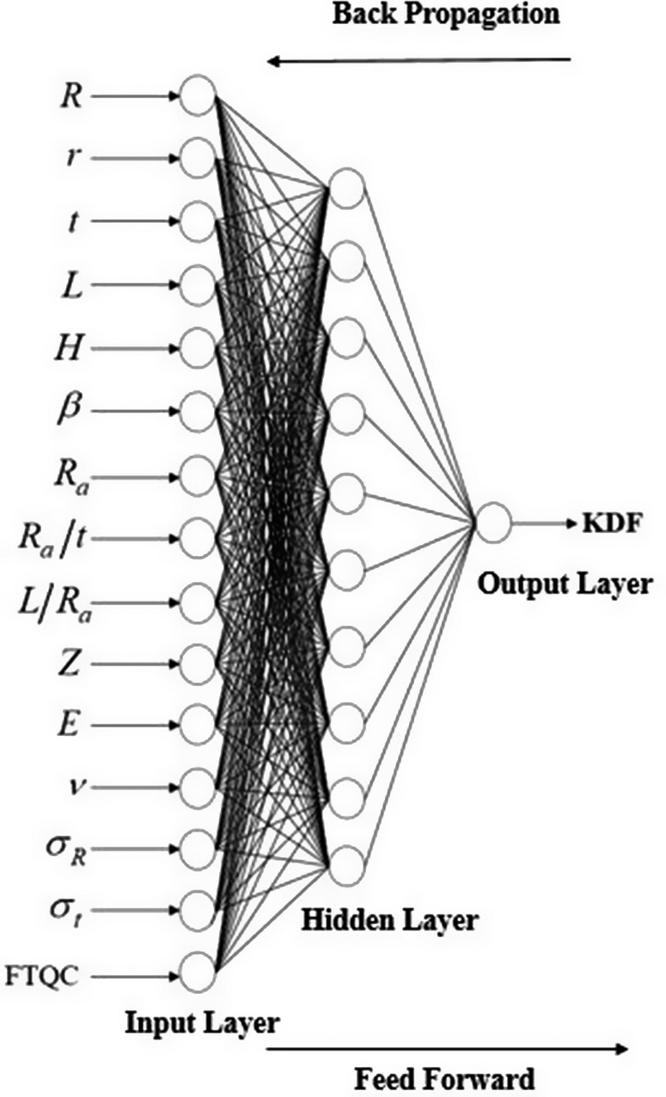
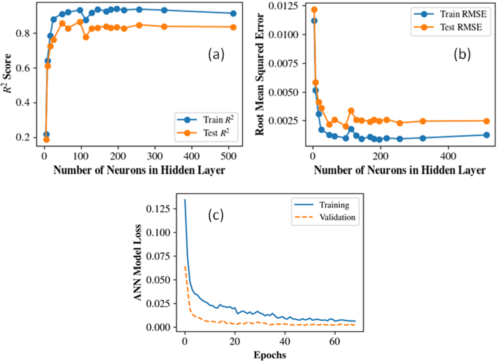
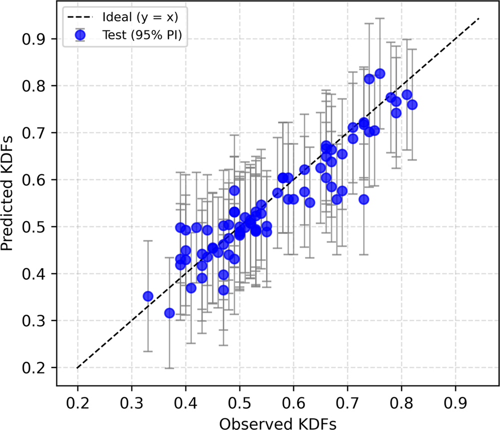
The ANN model was developed using the Keras API (Gulli and Pal, Reference Gulli and Pal2017) within the Python framework. A Rectified Linear Unit (ReLU) activation function (Dubey and Jain, Reference Dubey and Jain2019) was employed in the hidden layer, while a linear activation function was used in the single-neuron output layer to facilitate continuous value prediction. Training was carried out using the Adam optimizer (Zhang, Reference Zhang2018) with a learning rate of 10−3, and the root mean squared error (RMSE) was adopted as the loss function. The model was trained for up to 200 epochs using a batch size of 100. The Bayesian regularization algorithm was also employed. To mitigate overfitting, early stopping with a patience of 20 epochs was implemented, monitoring the validation loss and automatically restoring the weights corresponding to the best validation performance. During training, 10% of the dataset was allocated for validation. Figure 3a–3b shows the R2 and RMSE convergence plots that determined the choice of 256 hidden neurons. The model loss for training and validation against the number of epochs is also shown in Figure 3c. The ANN model predicted the KDFs in the test set with an R2 value of 0.841 along with a RMSE of 0.048. The prediction uncertainty was also quantified using split-conformal prediction intervals built from a held-out calibration split (20% of training data), giving distribution-free 95% prediction intervals (PI) for test predictions. Figure 4 shows the prediction performance of the ANN model on the test dataset. Predictions follow the (y = x) trend well across the main response range, with moderate dispersion around the diagonal and no obvious severe systematic bias. For quantification of uncertainty, an empirical coverage of 97.53% was observed with a mean interval width of 0.2355. This indicates the model is slightly conservative (coverage above nominal 95%), which is generally desirable for robustness. Overall, ANN provides good predictive accuracy with reliable and well-calibrated uncertainty bounds, making it suitable when both point prediction quality and interval reliability are important.
Convergence of (a) R2 and (b) RMSE for the ANN model to determine the optimal number of hidden neurons. (c) Training and validation model losses against the number of epochs.
KDF prediction performance of the ANN model on the test dataset.
2.2. SVR predictive model
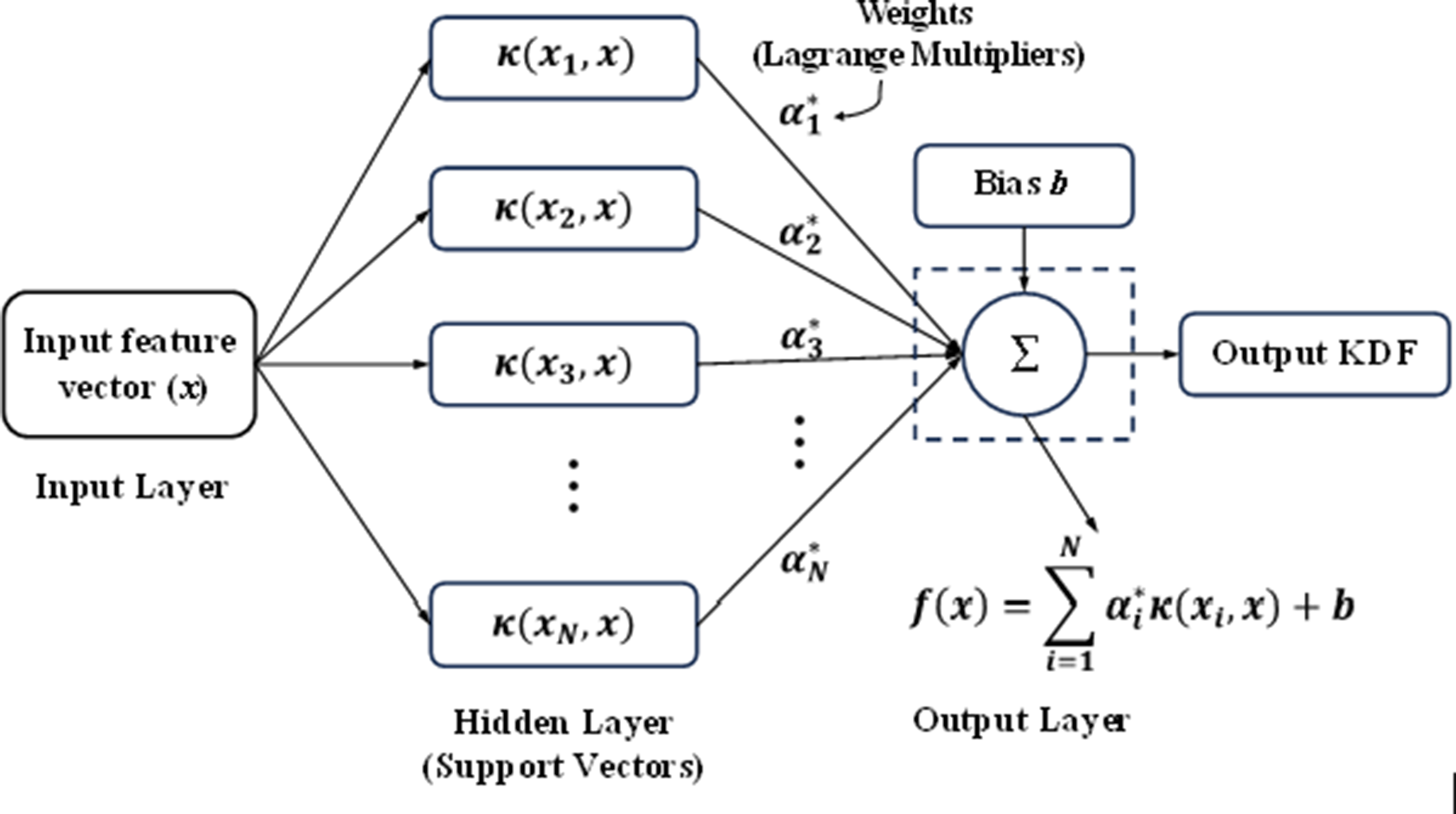
SVR is a regression-based extension of the support vector machine (SVM) framework (Zhang et al., Reference Zhang, Liu and Cao2024). It seeks to determine a function that captures the relationship between input features and target outputs while maintaining errors within a predefined tolerance limit, known as the ε-insensitive region. By applying a kernel function such as radial basis function (RBF), SVR projects the original input data into a higher-dimensional feature space, where a linear model is constructed to represent the underlying relationship. Figure 5 illustrates the general workflow of an SVR model. In this framework, the input vector
 $ x $
is transformed into a higher-dimensional feature space using kernel evaluations,
$ x $
is transformed into a higher-dimensional feature space using kernel evaluations,
 $ \kappa \left({x}_i,x\right) $
, calculated relative to each support vector
$ \kappa \left({x}_i,x\right) $
, calculated relative to each support vector
 $ {x}_i $
. The resulting kernel values are then scaled by their corresponding Lagrange multipliers,
$ {x}_i $
. The resulting kernel values are then scaled by their corresponding Lagrange multipliers,
 $ {\alpha}_i^{\ast } $
, and aggregated. Finally, the weighted sum is combined with the bias term
$ {\alpha}_i^{\ast } $
, and aggregated. Finally, the weighted sum is combined with the bias term
 $ b $
to generate the predicted regression output. SVR was established to predict the KDFs by optimizing a hyperplane that maintains deviations within a specified tolerance margin,
$ b $
to generate the predicted regression output. SVR was established to predict the KDFs by optimizing a hyperplane that maintains deviations within a specified tolerance margin,
 $ \varepsilon $
. The parameters for the SVR model were obtained through grid search optimization with a 5-fold CV, resulting in the adoption of a RBF kernel to effectively handle the nonlinear structure of the feature space. The model was configured with a regularization parameter of
$ \varepsilon $
. The parameters for the SVR model were obtained through grid search optimization with a 5-fold CV, resulting in the adoption of a RBF kernel to effectively handle the nonlinear structure of the feature space. The model was configured with a regularization parameter of
 $ C=20 $
, an epsilon tube of
$ C=20 $
, an epsilon tube of
 $ \varepsilon =0.01 $
, and a kernel coefficient of
$ \varepsilon =0.01 $
, and a kernel coefficient of
 $ \gamma =``\mathrm{scale}" $
(with polynomial degree = 2). To quantify the epistemic model uncertainty and evaluate robustness, which a standard SVR does not natively produce, a parametric bootstrap resampling approach was implemented. One hundred (
$ \gamma =``\mathrm{scale}" $
(with polynomial degree = 2). To quantify the epistemic model uncertainty and evaluate robustness, which a standard SVR does not natively produce, a parametric bootstrap resampling approach was implemented. One hundred (
 $ B=100 $
) independent SVR models were trained on random subsets of the training data sampled with replacement. The
$ B=100 $
) independent SVR models were trained on random subsets of the training data sampled with replacement. The
 $ 95\% $
confidence bounds for each prediction were then constructed using the 2.5th and 97.5th percentiles of the bootstrapped predictive distributions. Figure 6 shows the results of the SVR prediction on the test set with the 95% confidence interval (CI) vertical bars against each point estimate. When evaluated on the unseen test dataset, the model demonstrated robust generalization, yielding an
$ 95\% $
confidence bounds for each prediction were then constructed using the 2.5th and 97.5th percentiles of the bootstrapped predictive distributions. Figure 6 shows the results of the SVR prediction on the test set with the 95% confidence interval (CI) vertical bars against each point estimate. When evaluated on the unseen test dataset, the model demonstrated robust generalization, yielding an
 $ {R}^2 $
of 0.814, and a RMSE of 0.053. Despite providing reasonably accurate point estimates, the bootstrapped
$ {R}^2 $
of 0.814, and a RMSE of 0.053. Despite providing reasonably accurate point estimates, the bootstrapped
 $ 95\% $
CIs achieved a relatively low test-set empirical coverage of 54.3%, substantially lower than expected levels. The predicted CIs exhibit heterogeneous widths (signifying heteroscedasticity) across the KDF range. This implies that while the bootstrap aggregation accurately captured the variance attributable to finite training subsets, it underestimated the total predictive uncertainty (e.g., inherent data noise or systemic out-of-distribution behaviors), highlighting standard SVR’s limits in representing highly heteroscedastic regions of the structural response space.
$ 95\% $
CIs achieved a relatively low test-set empirical coverage of 54.3%, substantially lower than expected levels. The predicted CIs exhibit heterogeneous widths (signifying heteroscedasticity) across the KDF range. This implies that while the bootstrap aggregation accurately captured the variance attributable to finite training subsets, it underestimated the total predictive uncertainty (e.g., inherent data noise or systemic out-of-distribution behaviors), highlighting standard SVR’s limits in representing highly heteroscedastic regions of the structural response space.
General workflow (architecture) of SVR model.
KDF prediction performance of the SVR model on the test data.

2.3. RFR predictive model
RFR is an ensemble-based ML approach that integrates numerous decision trees (DTs) (Verma and Sharma, Reference Verma and Sharma2025) to enhance predictive performance and model stability. For estimating KDFs of conical shell structures, RFR provides an effective and relatively interpretable framework capable of capturing intricate, nonlinear interactions between geometric, material, and imperfection-related parameters and their influence on buckling strength reduction. The fundamental concept of RFR lies in constructing multiple DTs using randomly selected subsets of both input features and training samples (bootstrap aggregation). For each tree, the algorithm recursively selects the split (from the randomly selected subset of features) that minimizes the within-node mean-squared error. Terminal leaves then output the mean KDF of the training samples assigned to that leaf. The forest prediction is the ensemble mean across all trees, which reduces variance and improves generalization relative to a single DT. The generalized workflow is presented in Figure 7. In the present study, the RFR model was implemented using a bootstrap-aggregated ensemble of 500 regression trees (n_estimators = 500, bootstrap = True) with controlled complexity (max_depth = 20, min_samples_split = 5, min_samples_leaf = 1) and randomized feature sub-sampling at each split (max_features = 0.5). All the optimal hyperparameters were obtained through a randomized search with 5-fold CV. Using these tuned parameters, the developed model achieves a
 $ {R}^2 $
value of 0.834 and RMSE of 0.051 on the test data, indicating appreciable predictive capability and generalization as shown in Figure 8. It also shows the 95% CIs against each point estimate of the test KDFs. As evident from the vertical CI bounds, the range is smaller near the center of the distribution (KDFs between 0.5 and 0.7) while the dispersion increases as we move towards the tails. This can be attributed to less training data available near the tails and the model is less confident in its prediction. Since each DT in the forest predicts by averaging training targets in its terminal leaves, the RFR outputs are effectively constrained by the response values observed within the training domain. Consequently, when inputs fall outside the calibrated parameter space, predictions become less confident. An empirical 82.7% coverage on the test set was observed within the 95% CI bounds, suggesting appreciable reliability against KDF prediction.
$ {R}^2 $
value of 0.834 and RMSE of 0.051 on the test data, indicating appreciable predictive capability and generalization as shown in Figure 8. It also shows the 95% CIs against each point estimate of the test KDFs. As evident from the vertical CI bounds, the range is smaller near the center of the distribution (KDFs between 0.5 and 0.7) while the dispersion increases as we move towards the tails. This can be attributed to less training data available near the tails and the model is less confident in its prediction. Since each DT in the forest predicts by averaging training targets in its terminal leaves, the RFR outputs are effectively constrained by the response values observed within the training domain. Consequently, when inputs fall outside the calibrated parameter space, predictions become less confident. An empirical 82.7% coverage on the test set was observed within the 95% CI bounds, suggesting appreciable reliability against KDF prediction.
Random forest (RF) prediction framework comprising k individual DTs.

Performance of RFR predictive model with respect to test data.

2.4. HGB predictive model
Traditional boosting algorithms employ an ensemble strategy in which a sequence of DT models is constructed, with each successive tree attempting to reduce the errors of its predecessor. This is achieved by iteratively minimizing a predefined loss function using gradient descent. While such an approach is effective for many general datasets, it can become computationally expensive for complex problems because additional trees are progressively added to improve performance. Moreover, unlike RFR, conventional boosting methods do not naturally support parallel execution. To address these limitations, the HGB has been developed (Duc and Duc, Reference Duc and Duc2023). In HGB, continuous input features are first discretized into histogram bins, enabling approximate rather than exhaustive evaluation of potential split points. This binning process significantly lowers memory requirements and accelerates tree construction, while typically maintaining comparable predictive accuracy despite the coarser data representation. The block diagram of a typical HGB predictive model is shown in Figure 9. HGB models improve predictive accuracy and robustness within the training domain through gradient-based optimization and regularization. However, like RF, they rely on tree-based partitioning, which limits their ability to extrapolate. Predictions outside the calibrated range often follow the trend of terminal leaves near the boundary, resulting in moderate stability.
Workflow architecture (block diagram) of a typical HGB predictive model.

In this study, the HGB regressor was implemented in the Scikit-Learn library. Three parallel HGB models were run: one for the mean point prediction with “squared error” as the loss function, whereas the two remaining models (lower quantile: 0.025 and upper quantile: 0.975) were used for quantifying uncertainty of the KDF predictions with interval-order corrections applied to prevent quantile crossing. For all component models, the optimal hyperparameters were identified through a 5-fold grid search-based CV. The finalized configuration included a maximum of 500 boosting iterations, with each successive tree correcting the residuals of the previous ensemble using a learning rate of 0.1. Model complexity was controlled by limiting the maximum tree depth to 20, and overfitting was mitigated by considering only 10% of the available features at each split. The model achieved
 $ {R}^2 $
and RMSE values of 0.832 and 0.050, respectively, for the testing dataset. Overall, the HGB model shows promising predictive capabilities signified by the tighter scatter around the y = x line for low-to-mid KDF range, with a larger spread at higher observed values. Regarding the quantification of prediction uncertainty, the 95% CI bands for HGB could capture an empirical coverage of 70.4% on the test set despite a relatively narrow mean test interval (about 0.124), indicating slightly overconfident bounds under test conditions. While this coverage is better than the SVR model, it is less than the RFR model. Overall, the HGB framework is robust and effective as a deterministic regressor in this dataset, but its native quantile intervals are inadequately calibrated for reliable 95% confidence claims. Figure 10 illustrates the predictive capability of the HGB model with respect to the test dataset.
$ {R}^2 $
and RMSE values of 0.832 and 0.050, respectively, for the testing dataset. Overall, the HGB model shows promising predictive capabilities signified by the tighter scatter around the y = x line for low-to-mid KDF range, with a larger spread at higher observed values. Regarding the quantification of prediction uncertainty, the 95% CI bands for HGB could capture an empirical coverage of 70.4% on the test set despite a relatively narrow mean test interval (about 0.124), indicating slightly overconfident bounds under test conditions. While this coverage is better than the SVR model, it is less than the RFR model. Overall, the HGB framework is robust and effective as a deterministic regressor in this dataset, but its native quantile intervals are inadequately calibrated for reliable 95% confidence claims. Figure 10 illustrates the predictive capability of the HGB model with respect to the test dataset.
Performance of the HGB predictive model with respect to test data.

2.5. Hybrid (GPR + XGB) predictive model
The GPR has been successfully implemented in many domains of engineering and science for probabilistic predictions and quantifying uncertainties (Le and Le, Reference Le and Le2021; Assolie, Reference Assolie2024). GPR can estimate full distributions with means and dispersions rather than a single predicted value and offers flexibility through the use of kernel-based inductive biases that align well with shell buckling behavior (smooth but with localized imperfections). However, for complex nonlinear interdependencies within the features and observations, its capabilities can be challenged. The XGB algorithm (Ali and Burhan, Reference Ali and Burhan2023) is known for its robustness and efficiency for handling highly nonlinear relationships. XGB also reduces bias through boosted ensembles and performs well under noisy features. Therefore, in this study, a hybrid two-stage Gaussian Process-XG Boost (GPR + XGB) regressor is proposed, which combines the complementary strengths of both algorithms, enabling improved predictive performance for estimating the KDFs. The hybrid model is a residual-learning architecture where GPR is the base learner, and XGB is the residual corrector. Conceptually, it models the KDFs (predicted) as shown in Equation 4
 $$ {KDF}_{pred}={f}_{GPR}(x)+{f}_{XGB}\left(x,{\mu}_{GPR},{\sigma}_{GPR}\right)+\varepsilon $$
where,
 $ {f}_{GPR}(x) $
captures the smooth global response surface of the KDFs with respect to the input features (x), and then the second-stage
$ {f}_{GPR}(x) $
captures the smooth global response surface of the KDFs with respect to the input features (x), and then the second-stage
 $ {f}_{XGB}\left(x,{\mu}_{GPR},{\sigma}_{GPR}\right) $
learns the structured residual component that remains unexplained by the kernel model, thereby yielding a final predictor. Schematically, the entire workflow of the proposed hybrid model is shown in Figure 11 and a detailed description of the steps is provided next.
$ {f}_{XGB}\left(x,{\mu}_{GPR},{\sigma}_{GPR}\right) $
learns the structured residual component that remains unexplained by the kernel model, thereby yielding a final predictor. Schematically, the entire workflow of the proposed hybrid model is shown in Figure 11 and a detailed description of the steps is provided next.
Workflow of the proposed hybrid (GPR + XGB) predictive model (architecture).

In the first stage, the Gaussian Process kernel was constructed as a composite covariance function, as shown in Equation 5.
 $$ k\left(x,{x}^{\prime}\right)=C\ast {k}_{Matern,\nu =2.5}\left(x,{x}^{\prime}\right)+{k}_{white}\left(x,{x}^{\prime}\right) $$
where the constant Kernel (C) scaled the overall signal variance, the Matern component captured smooth but not overly rigid structure in the response, and the White Kernel explicitly modelled observation-level noise. The GPR model was then fit on the training set (split into train and validation folds) through an Out-of-Fold (OOF, 5-fold) loop. Four folds were used to train the GPR and predict only the held-out fold, repeated across all folds so that every training sample receives a prediction from a model that did not see that sample during fitting. These OOF predictions were then used to construct leakage-free residual targets
 $ {r}_{train}={KDF}_{train}-{\mu}_{OOF} $
and uncertainty features (
$ {r}_{train}={KDF}_{train}-{\mu}_{OOF} $
and uncertainty features (
 $ {\sigma}_{OOF}\Big) $
.The meta features (
$ {\sigma}_{OOF}\Big) $
.The meta features (
 $ {\mu}_{OOF},{\sigma}_{OOF} $
) were appended to the training feature set to generate an uncertainty-informed stacked design matrix for the XGB residual learner, ensuring that stage-two training reflected realistic generalization error rather than optimistically biased in-sample fit as given in Equation 6.
$ {\mu}_{OOF},{\sigma}_{OOF} $
) were appended to the training feature set to generate an uncertainty-informed stacked design matrix for the XGB residual learner, ensuring that stage-two training reflected realistic generalization error rather than optimistically biased in-sample fit as given in Equation 6.
 $$ {X}_{train,\hskip0.36em stacked}=\left[{X}_{train},{\mu}_{OOF},{\sigma}_{OOF}\right] $$
Consequently, the OOF mechanism improved the statistical validity of residual stacking and supports more reliable downstream uncertainty calibration. Additionally, residual-model fitting was weighted by (
 $ {w}_i=\frac{1}{1+{\sigma}_{OOF,i}^2}\Big) $
so that observations with higher epistemic uncertainty had proportionally lower influence during XGB optimization. Hyperparameters of the XGB learner were selected by randomized cross-validated search (using
$ {w}_i=\frac{1}{1+{\sigma}_{OOF,i}^2}\Big) $
so that observations with higher epistemic uncertainty had proportionally lower influence during XGB optimization. Hyperparameters of the XGB learner were selected by randomized cross-validated search (using
 $ {X}_{train,\hskip0.36em stacked} $
and
$ {X}_{train,\hskip0.36em stacked} $
and
 $ {r}_{train} $
) over tree depth, learning rate, subsampling, column sampling, regularization, and number of estimators and their optimal values were 6, 0.02, 0.75, 0.75, 2, and 2000 respectively. For the test set, one final GPR was fit on the entire training set to predict the mean and standard deviation for the test set, which was subsequently stacked with the test features to obtain the stacked test features (Equation 7).
$ {r}_{train} $
) over tree depth, learning rate, subsampling, column sampling, regularization, and number of estimators and their optimal values were 6, 0.02, 0.75, 0.75, 2, and 2000 respectively. For the test set, one final GPR was fit on the entire training set to predict the mean and standard deviation for the test set, which was subsequently stacked with the test features to obtain the stacked test features (Equation 7).
 $$ {X}_{test,\hskip0.36em stacked}=\left[{X}_{test},{\mu}_{test},{\sigma}_{test}\right] $$
The tuned XGB model was then used to predict the residuals for the test set (Equation 8),
 $$ {\overset{}{r\check{}}}_{test}={f}_{XGB}\left({X}_{test,\hskip0.36em stacked}\right) $$
The final hybrid KDF prediction model was then developed (Equation 9).
 $$ {\hat{KDF}}_{test}={\mu}_{test}+{\overset{}{r\check{}}}_{test} $$
To quantify predictive uncertainty on unseen data, split-conformal prediction intervals were constructed using absolute out-of-fold hybrid residuals, with finite-sample calibrated quantile correction to produce nominal 95% intervals. This hybrid strategy delivered the strongest predictive accuracy amongst the other tested alternatives, achieving a final meta-model test performance of R2 of 0.867 and RMSE of 0.04, exceeding the performances of the RFR, SVR, ANN, and HGB models. The empirical uncertainty coverage was 97.5%, which was at par with the ANN model and considerably better than the rest. This superiority is consistent with the intended bias-variance decomposition of the framework, where GPR provides globally coherent function approximation and calibrated local uncertainty descriptors, and XGB adaptively corrects high-order nonlinear residual structure that a kernel-only model may leave unresolved. Figure 12 shows the performance of the (GPR + XGB) model on the test dataset.
Hybrid (GPR + XGB) predictive model performance on test data.

3. Performance measurement of various ML predictive models
In this section, a detailed comparison of the different ML models used in this study is discussed. Table 3 shows the performance comparison of all the ML models used in the KDF predictions through various metrics like R2, RMSE, MAE (mean absolute error), explained variance, and 95% CI coverage.
Performance summary of different ML predictive models
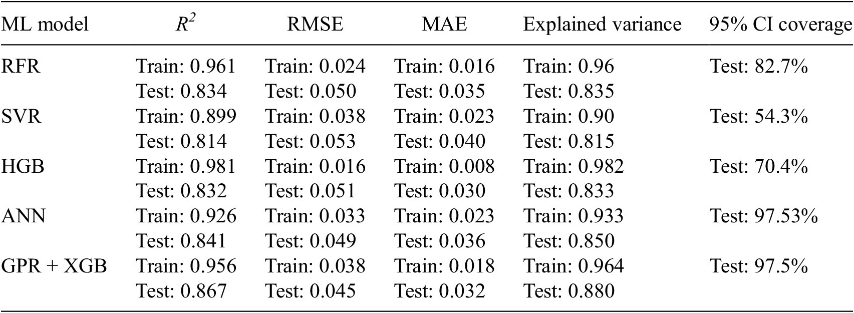
The comparative evaluation of the five ML models demonstrates a clear hierarchy in predictive fidelity, generalization behavior, and uncertainty reliability for KDF estimations. Among all predictive models, the hybrid GPR + XGB model delivered the strongest overall test performance, achieving the highest coefficient of determination (
 $ {R}^2=0.867 $
), the lowest RMSE (0.045), and the highest explained variance (0.880), while maintaining low MAE (0.032), indicating that it most effectively captured both the central trend and global variance structure of the KDF response. The ANN model ranked second overall (
$ {R}^2=0.867 $
), the lowest RMSE (0.045), and the highest explained variance (0.880), while maintaining low MAE (0.032), indicating that it most effectively captured both the central trend and global variance structure of the KDF response. The ANN model ranked second overall (
 $ {R}^2=0.841 $
, RMSE = 0.049, MAE = 0.036, explained variance = 0.850), showing consistently strong predictive skill and only marginal degradation relative to the best model, whereas RFR and HGB formed an intermediate tier. RFR exhibited balanced but weaker performance (
$ {R}^2=0.841 $
, RMSE = 0.049, MAE = 0.036, explained variance = 0.850), showing consistently strong predictive skill and only marginal degradation relative to the best model, whereas RFR and HGB formed an intermediate tier. RFR exhibited balanced but weaker performance (
 $ {R}^2=0.834 $
, RMSE = 0.050, MAE = 0.035, explained variance = 0.835), while HGB achieved the lowest MAE (0.030), suggesting high accuracy around the conditional median, but lower
$ {R}^2=0.834 $
, RMSE = 0.050, MAE = 0.035, explained variance = 0.835), while HGB achieved the lowest MAE (0.030), suggesting high accuracy around the conditional median, but lower
 $ {R}^2 $
(0.832) and explained variance (0.833), highlighting reduced ability to reproduce full KDF response dispersion. SVR was the least competitive model (
$ {R}^2 $
(0.832) and explained variance (0.833), highlighting reduced ability to reproduce full KDF response dispersion. SVR was the least competitive model (
 $ {R}^2=0.814 $
, RMSE = 0.053, MAE = 0.040, explained variance = 0.815), reflecting comparatively limited nonlinear representational adequacy under the present tuning and data regime. Train-test contrasts further suggest that ensemble tree boosting models (especially HGB) experienced larger generalization drops from training to testing, consistent with a stronger overfitting tendency despite excellent in-sample fit, whereas GPR + XGB and ANN retained superior out-of-sample stability. Importantly, uncertainty quantification results reinforced this ranking, that is 95% confidence-interval coverage was near nominal for ANN (97.53%) and GPR + XGB (97.5%), implying well-calibrated, slightly conservative KDF predictive intervals suitable for reliability-oriented contexts, but in contrast, RFR (82.7%), HGB (70.4%), and SVR (54.3%) substantially under-covered the observations, indicating overconfident intervals and underestimated epistemic/aleatoric spread. Collectively, these findings indicate that the GPR + XGB model provides the best overall compromise between deterministic accuracy and probabilistic trustworthiness, the ANN model offers a highly competitive alternative with similarly strong calibration capabilities, and the SVR is comparatively the least suitable for this KDF prediction task in its current configuration.
$ {R}^2=0.814 $
, RMSE = 0.053, MAE = 0.040, explained variance = 0.815), reflecting comparatively limited nonlinear representational adequacy under the present tuning and data regime. Train-test contrasts further suggest that ensemble tree boosting models (especially HGB) experienced larger generalization drops from training to testing, consistent with a stronger overfitting tendency despite excellent in-sample fit, whereas GPR + XGB and ANN retained superior out-of-sample stability. Importantly, uncertainty quantification results reinforced this ranking, that is 95% confidence-interval coverage was near nominal for ANN (97.53%) and GPR + XGB (97.5%), implying well-calibrated, slightly conservative KDF predictive intervals suitable for reliability-oriented contexts, but in contrast, RFR (82.7%), HGB (70.4%), and SVR (54.3%) substantially under-covered the observations, indicating overconfident intervals and underestimated epistemic/aleatoric spread. Collectively, these findings indicate that the GPR + XGB model provides the best overall compromise between deterministic accuracy and probabilistic trustworthiness, the ANN model offers a highly competitive alternative with similarly strong calibration capabilities, and the SVR is comparatively the least suitable for this KDF prediction task in its current configuration.
3.1. Data sparsity analysis and distribution of prediction error
To assess whether the KDF predictive accuracy degrades in regions with limited data support, a Kernel density estimation (KDE) based sparsity analysis was conducted on the GPR + XGB test predictions. A Gaussian kernel density model was fitted on the training set, and each test sample was assigned a sparsity score defined as the negative log-density, such that larger values indicate lower local support as given in Equation 9.1 and 9.2 respectively.
 $$ {s}_i=-\log \hat{p}\left({x}_{test,i}\right) $$
 $$ \hat{p}(x)=\frac{1}{n_{train}}\sum \limits_{j=1}^{n_{train}}k\left(x,{x}_j^{train}\right) $$
where, k is the Gaussian kernel. Test errors were then examined globally and across sparsity quintiles (Q1: densest to Q5: sparsest). The GPR + XGB model retained strong aggregate performance (RMSE = 0.0447, MAE = 0.0325), and the association between absolute error and sparsity was mildly negative (Spearman’s correlation
 $ \rho =-0.308 $
), indicating that larger errors did not systematically accumulate in sparse data regions. Stratification by KDE-based sparsity quintiles revealed a non-monotonic error pattern: performance was strongest in Q4 (RMSE = 0.0277), moderate in Q2 and Q3 (RMSE = 0.0510 and 0.0402, respectively), and degraded most in Q1 (RMSE = 0.0596). Interestingly, it was observed that the RMSE kept decreasing till Q4, and for the rarest quintile, Q5, RMSE again increased to 0.0361. Consistent with this, the stacked RMSE distribution remained centered near the zero-error reference, without considerable systematic bias. The KDF prediction error appeared to be heterogeneous but not concentrated in the sparsest regime, with the densest groups exhibiting comparatively larger errors. Altogether, these results suggest that, for the present train-test dataset, performance variation was driven more by localized KDF response complexity than by sparsity alone, and that refinement should be aimed at specific high-error subregions rather than sparsity bins in general. The prediction error distribution is shown in Figure 13.
$ \rho =-0.308 $
), indicating that larger errors did not systematically accumulate in sparse data regions. Stratification by KDE-based sparsity quintiles revealed a non-monotonic error pattern: performance was strongest in Q4 (RMSE = 0.0277), moderate in Q2 and Q3 (RMSE = 0.0510 and 0.0402, respectively), and degraded most in Q1 (RMSE = 0.0596). Interestingly, it was observed that the RMSE kept decreasing till Q4, and for the rarest quintile, Q5, RMSE again increased to 0.0361. Consistent with this, the stacked RMSE distribution remained centered near the zero-error reference, without considerable systematic bias. The KDF prediction error appeared to be heterogeneous but not concentrated in the sparsest regime, with the densest groups exhibiting comparatively larger errors. Altogether, these results suggest that, for the present train-test dataset, performance variation was driven more by localized KDF response complexity than by sparsity alone, and that refinement should be aimed at specific high-error subregions rather than sparsity bins in general. The prediction error distribution is shown in Figure 13.
Distribution of prediction errors across density-based quintiles (Q1–Q5).

3.2. Validation and performance assessment of the hybrid (GPR + XGB) model
A comparison of the proposed (GPR + XGB) predictive model with the actual results from a validation dataset (different from T&T) is shown in Figure 14. A
 $ {R}^2 $
and RMSE of 0.88 and 0.043, respectively, were attained on these external validation data. The verification dataset consisted of 20 (twenty) simulated points different from the T&T data.
$ {R}^2 $
and RMSE of 0.88 and 0.043, respectively, were attained on these external validation data. The verification dataset consisted of 20 (twenty) simulated points different from the T&T data.
(a) Comparison of the proposed (GPR + XGB) predictive model with actual KDFs on validation data different from T&T.

The (GPR + XGB) hybrid model predicts the KDFs with a high degree of accuracy, closely matching the experimental and simulated KDF values. Consequently, it can be confidently employed within the parametric bounds used during the network training phase. A strong and excellent agreement between the actual and the proposed (GPR + XGB) hybrid ML predicted KDFs was observed when tested on an additional validation data. Code prescribed KDFs such as those stipulated by NASA: SP-8019 (Weingarten and Seide, Reference Weingarten and Seide1968), Euro code (EC 3) (ECCS, 2008), energy barrier criterion (EBC) (Wagner et al., Reference Wagner, Huhne and Khakimova2018) and so forth were also included as discrete markers as shown in Figure 15. The alternative threshold KDF, as predicted by the energy barrier criterion (EBC) is shown in Equation 10 as a function of
 $ Z $
(Wagner et al., Reference Wagner, Huhne and Khakimova2018).
$ Z $
(Wagner et al., Reference Wagner, Huhne and Khakimova2018).
 $$ {KDF}_{EBC}=1.07{(Z)}^{-0.138};50\le Z\le 7000 $$
Comparative evaluation of code-recommended and the hybrid (GPR + XGB) ML predicted KDFs on a validation dataset different from T&T.

Such code-specified values consistently appear at markedly lower magnitudes compared to the proposed (GPR + XGB) based predictions, underscoring the inherent conservatism of the existing design formulations. The code-based KDFs were observed to be significantly conservative, typically underestimating the actual KDFs by approximately 20%—30%. Amongst the available design provisions, NASA SP-8019 (Weingarten and Seide, Reference Weingarten and Seide1968) yields the most conservative KDF value (0.33), regardless of the shell geometry considered. The threshold KDFs and those derived from the EBC proposed by Wagner et al. (Reference Wagner, Huhne and Khakimova2018) provides a slight improvement over the NASA recommendation, primarily due to the inclusion of additional influencing parameters in their formulation. In contrast, Eurocode (EC-3) (ECCS, 2008) accounts for fabrication quality through the FTQC classification, which leads to comparatively less conservative KDF values than the other code-based stipulations. Overall, the KDFs predicted by the proposed hybrid model (GPR + XG Boost) show the highest accuracy and least conservatism.
3.3. Sensitivity to training-set size
The predictive performance of the developed ML models exhibits a clear dependence on the size and richness of the training dataset. As highlighted in the study, models trained on limited experimental data alone would suffer from higher variance and reduced generalization capability. However, the incorporation of a larger, heterogeneous dataset (experimental + simulated) significantly enhances robustness and prediction accuracy. Complex nonlinear models such as ANN, RFR, HGB, and particularly the hybrid (GPR + XGB) framework benefit substantially from increased training data, as larger datasets enable better learning of intricate feature interactions governing buckling behavior. Conversely, in data-sparse regimes, model predictions become more sensitive to sampling variability, leading to increased epistemic uncertainty, as reflected through cross-validation variability and reduced confidence in extrapolated regions. The study mitigates this sensitivity through strategies such as 5-fold CV, ensemble learning, and uncertainty-aware modelling, which improve data efficiency and stabilize predictions. Overall, the findings emphasize that aligning model complexity with available data is crucial as richer datasets unlock the full potential of advanced ML models, whereas data-limited scenarios require regularization and hybrid strategies to maintain reliability.
4. Sensitivity assessment using the proposed (GPR + XGB) model
The relative contribution of each input parameter toward the accuracy of KDF prediction was also carried out through a detailed sensitivity analysis, as illustrated in Table 4. This assessment adopted a leave-one-variable-out approach, where individual input parameters were sequentially removed while all remaining variables were retained. The hybrid predictive model, i.e., (GPR + XGB), was adopted for this investigation, as it demonstrated the highest predictive accuracy amongst all the considered ML models as discussed before. For each reduced feature set, the performance of the (GPR + XGB) hybrid model was re-evaluated using RMSE and
 $ {R}^2 $
as a performance indicator. The corresponding changes in RMSE,
$ {R}^2 $
as a performance indicator. The corresponding changes in RMSE,
 $ {R}^2 $
as presented in Table 4, served as quantitative measures of the model’s sensitivity to specific input parameters. The study was carried out to identify the most critical geometric feature (parameter) affecting the KDF. Hence, only the geometric parameters were included in the sensitivity analysis. A significant rise in RMSE, together with a decline in
$ {R}^2 $
as presented in Table 4, served as quantitative measures of the model’s sensitivity to specific input parameters. The study was carried out to identify the most critical geometric feature (parameter) affecting the KDF. Hence, only the geometric parameters were included in the sensitivity analysis. A significant rise in RMSE, together with a decline in
 $ {R}^2 $
upon exclusion of a given feature, signified its substantial contribution to the model’s predictive capability. In contrast, minimal variations in these metrics implied a relatively limited influence of that parameter on KDF estimation. Furthermore, the sensitivity analysis offered meaningful physical insight into the problem, facilitating the identification of key governing factors and providing direction for future data collection, model refinement, and design-oriented implementation.
$ {R}^2 $
upon exclusion of a given feature, signified its substantial contribution to the model’s predictive capability. In contrast, minimal variations in these metrics implied a relatively limited influence of that parameter on KDF estimation. Furthermore, the sensitivity analysis offered meaningful physical insight into the problem, facilitating the identification of key governing factors and providing direction for future data collection, model refinement, and design-oriented implementation.
Sensitivity analysis through the proposed hybrid (GPR + XGB) ML predictive model with respect to
 $ {R}^2 $
and RMSE
$ {R}^2 $
and RMSE
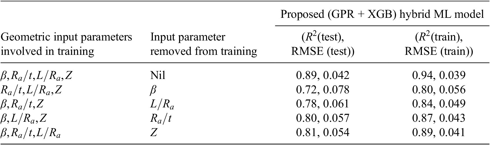
Upon removing
 $ \beta $
, the model performance degraded significantly, with
$ \beta $
, the model performance degraded significantly, with
 $ {R}^2 $
dropping to 0.72 and RMSE increasing to 0.078, indicating that
$ {R}^2 $
dropping to 0.72 and RMSE increasing to 0.078, indicating that
 $ \beta $
is the most influential parameter in governing the KDF prediction. The exclusion of
$ \beta $
is the most influential parameter in governing the KDF prediction. The exclusion of
 $ L/{R}_a $
also led to a notable reduction in accuracy
$ L/{R}_a $
also led to a notable reduction in accuracy
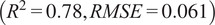 $ \left({R}^2=0.78, RMSE=0.061\right) $
confirming the strong contribution of the slenderness ratio to shell behavior. Similarly, removing
$ \left({R}^2=0.78, RMSE=0.061\right) $
confirming the strong contribution of the slenderness ratio to shell behavior. Similarly, removing
 $ {R}_a/t $
reduced the predictive capability to
$ {R}_a/t $
reduced the predictive capability to
 $ {R}^2=0.8 $
with RMSE = 0.057, demonstrating the importance of thickness-related effects in stability response. In contrast, eliminating
$ {R}^2=0.8 $
with RMSE = 0.057, demonstrating the importance of thickness-related effects in stability response. In contrast, eliminating
 $ Z $
resulted in only a moderate change in performance
$ Z $
resulted in only a moderate change in performance
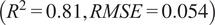 $ \left({R}^2=0.81, RMSE=0.054\right) $
, suggesting a comparatively lower influence. Overall, the sensitivity ranking can be inferred as
$ \left({R}^2=0.81, RMSE=0.054\right) $
, suggesting a comparatively lower influence. Overall, the sensitivity ranking can be inferred as
 $ \beta $
being the most dominant parameter, followed by
$ \beta $
being the most dominant parameter, followed by
 $ L/{R}_a $
,
$ L/{R}_a $
,
 $ {R}_a/t $
and
$ {R}_a/t $
and
 $ Z $
. However, the mechanical properties
$ Z $
. However, the mechanical properties
 $ E $
and
$ E $
and
 $ \upsilon $
does not significantly affect KDFs as compared to geometric properties (Majumder et al., Reference Majumder, Chakraborty and Mishra2023). This is also represented through sensitivity plots as shown in Figure 16a–16b.
$ \upsilon $
does not significantly affect KDFs as compared to geometric properties (Majumder et al., Reference Majumder, Chakraborty and Mishra2023). This is also represented through sensitivity plots as shown in Figure 16a–16b.
Sensitivity analysis by adopting a leave-one-variable-out approach with respect to (a)
 $ {R}^2 $
and (b) RMSE.
$ {R}^2 $
and (b) RMSE.

The dominance of
 $ \beta $
on KDFs is also established in the classical buckling theory (Chryssanthopoulus et al., Reference Chryssanthopoulus, Poggi and Spagnoli1998; Maiorana et al., Reference Maiorana, Aloisio and Briseghella2023) which is once again presented here through the sensitivity study. These findings confirm that the hybrid model effectively captured the nonlinear relationships among the geometric variables while also providing meaningful insight into the governing parameters affecting KDF prediction. Variations in the geometric properties
$ \beta $
on KDFs is also established in the classical buckling theory (Chryssanthopoulus et al., Reference Chryssanthopoulus, Poggi and Spagnoli1998; Maiorana et al., Reference Maiorana, Aloisio and Briseghella2023) which is once again presented here through the sensitivity study. These findings confirm that the hybrid model effectively captured the nonlinear relationships among the geometric variables while also providing meaningful insight into the governing parameters affecting KDF prediction. Variations in the geometric properties
 $ \left(\beta, {R}_a/t,Z\right) $
plays a significant role in the KDF estimation as shown through partial dependence plots (PDPs) for the hybrid (GPR + XGB) predictive model, as shown in Figure 17a–17c. PDP explains about a feature that influences the prediction of an ML model while averaging out the effects of other features.
$ \left(\beta, {R}_a/t,Z\right) $
plays a significant role in the KDF estimation as shown through partial dependence plots (PDPs) for the hybrid (GPR + XGB) predictive model, as shown in Figure 17a–17c. PDP explains about a feature that influences the prediction of an ML model while averaging out the effects of other features.
PDPs with respect to (a)
 $ \beta $
, (b)
$ \beta $
, (b)
 $ {R}_a/t $
and (c)
$ {R}_a/t $
and (c)
 $ Z $
.
$ Z $
.

Overall, the plots confirm that
 $ \beta, {R}_a/t $
and
$ \beta, {R}_a/t $
and
 $ Z $
have a strong non-linear negative influence on KDFs.
$ Z $
have a strong non-linear negative influence on KDFs.
5. Conclusion
The present study develops a comprehensive data-driven framework for predicting the buckling KDFs of thin-walled truncated conical shells subjected to axial compression. Recognizing the long-standing discrepancy between theoretical and experimentally observed buckling loads and the excessive conservatism embedded in traditional design codes, this work systematically evaluates multiple ML algorithms, including ANN, SVR, RFR, HGB, and a novel (GPR + XGB) hybrid model. A heterogeneous dataset comprising 400 samples (after outlier removal) derived from both experimental investigations and nonlinear FE simulations are utilized for model T&T under a rigorous 5-fold CV framework. Among all considered models, the proposed hybrid (GPR + XGB) framework demonstrates the highest predictive accuracy, achieving an
 $ {R}^2 $
of 0.867 and RMSE of 0.045 on the test data. The hybrid strategy effectively combines the probabilistic, uncertainty-quantifying capability of GPR with the strong nonlinear learning and residual correction strength of XGB. Comparative evaluation reveals that the hybrid model consistently outperforms individual ML models and significantly reduces the conservatism inherent in code-based KDF recommendations such as NASA SP-8019 and EC-3 provisions. Code-specified KDFs are found to underestimate actual values by nearly 20%–30%, whereas the proposed hybrid-based predictions show excellent agreement with experimental and simulated results. The sensitivity analysis conducted using a leave-one-variable-out approach further establishes
$ {R}^2 $
of 0.867 and RMSE of 0.045 on the test data. The hybrid strategy effectively combines the probabilistic, uncertainty-quantifying capability of GPR with the strong nonlinear learning and residual correction strength of XGB. Comparative evaluation reveals that the hybrid model consistently outperforms individual ML models and significantly reduces the conservatism inherent in code-based KDF recommendations such as NASA SP-8019 and EC-3 provisions. Code-specified KDFs are found to underestimate actual values by nearly 20%–30%, whereas the proposed hybrid-based predictions show excellent agreement with experimental and simulated results. The sensitivity analysis conducted using a leave-one-variable-out approach further establishes
 $ \beta $
as the most influential geometric parameter governing KDF prediction is, followed by slenderness-related and thickness-dependent parameters. The findings are consistent with classical shell buckling theory, thereby reinforcing the physical reliability of the proposed hybrid model. Overall, the study demonstrates that a hybrid (GPR + XGB) predictive framework integrating experimental evidence, simulated data, and uncertainty-aware modelling can provide accurate, robust, and less conservative KDF predictions.
$ \beta $
as the most influential geometric parameter governing KDF prediction is, followed by slenderness-related and thickness-dependent parameters. The findings are consistent with classical shell buckling theory, thereby reinforcing the physical reliability of the proposed hybrid model. Overall, the study demonstrates that a hybrid (GPR + XGB) predictive framework integrating experimental evidence, simulated data, and uncertainty-aware modelling can provide accurate, robust, and less conservative KDF predictions.
6. Future scope of research
From the probabilistic design point of view, the permissible/allowable
 $ \beta $
for achieving a target reliability index
$ \beta $
for achieving a target reliability index
 $ \left(\gamma \right) $
(or failure probability
$ \left(\gamma \right) $
(or failure probability
 $ {p}_f $
) (Haldar and Mahadevan, Reference Haldar and Mahadevan2000), using specific (or safety consistent) KDFs may be carried out as a part of future research work. Such allowable
$ {p}_f $
) (Haldar and Mahadevan, Reference Haldar and Mahadevan2000), using specific (or safety consistent) KDFs may be carried out as a part of future research work. Such allowable
 $ \beta $
s, which are to be treated as the design variables (DVs) may be enforced for quality control during the manufacturing process of conical shells. Also, as a prospective extension of the current study, PINNs may be adopted to offer a robust framework for prediction in systems governed by established physical laws, particularly in situations where experimental data are scarce or costly to obtain. By embedding governing equations directly into the learning process, PINNs enhance model generalization and improve extrapolation capability beyond the training domain. Their physics-based constraints enable more reliable predictions outside the calibration range, making them especially suitable for applications requiring physically consistent outcomes. Therefore, the proposed approach in the study offers a more rational basis for more economical and reliability-consistent buckling design of conical shells and lays the foundation for future extensions toward physics-informed and probabilistic design methodologies.
$ \beta $
s, which are to be treated as the design variables (DVs) may be enforced for quality control during the manufacturing process of conical shells. Also, as a prospective extension of the current study, PINNs may be adopted to offer a robust framework for prediction in systems governed by established physical laws, particularly in situations where experimental data are scarce or costly to obtain. By embedding governing equations directly into the learning process, PINNs enhance model generalization and improve extrapolation capability beyond the training domain. Their physics-based constraints enable more reliable predictions outside the calibration range, making them especially suitable for applications requiring physically consistent outcomes. Therefore, the proposed approach in the study offers a more rational basis for more economical and reliability-consistent buckling design of conical shells and lays the foundation for future extensions toward physics-informed and probabilistic design methodologies.
Data availability statement
The data supporting this study are adopted from published literature and are available at the following DOIs: https://doi.org/10.1016/j.ijmecsci.2018.07.016 and https://doi.org/10.1016/j.tws.2024.112541. The compiled data employed for T&T is also submitted as a supplementary material.
Author contribution
R.M.: conceptualization (lead), data curation (lead), formal analysis (lead), investigation (equal), writing original draft (lead). B.D.: investigation (equal), resources (equal), software (equal), validation (equal), writing – reviewing and editing (equal). A.D.G.: data curation (equal), investigation (equal), validation (equal), writing original draft (supporting). S.K.M.: supervision (lead), writing – reviewing and editing (equal).
Funding statement
The authors would like to acknowledge the SEED Grant (Ref No. AU/SRG/2025–01) received from Adani University, Ahmedabad, in carrying out the research.
Competing interests
The authors declare none.
A. Appendix
A.1. FE-Based buckling analysis of truncated conical shell with axial compression
A thin truncated conical shell is considered with
 $ R $
= 400 mm,
$ R $
= 400 mm,
 $ r $
=190 mm,
$ r $
=190 mm,
 $ t $
= 0.75 mm,
$ t $
= 0.75 mm,
 $ \beta $
= 35° and
$ \beta $
= 35° and
 $ L $
= 366.23 mm. The shell is made of Al 6061-T6 aluminum alloy, having a density
$ L $
= 366.23 mm. The shell is made of Al 6061-T6 aluminum alloy, having a density
 $ \left(\rho \right) $
of 2700 kg/m3,
$ \left(\rho \right) $
of 2700 kg/m3,
 $ E $
= 68.9 GPa,
$ E $
= 68.9 GPa,
 $ \upsilon $
= 0.33 and a yield stress
$ \upsilon $
= 0.33 and a yield stress
 $ (Y) $
of 240 MPa. The truncated conical shell is modeled with its base fully clamped in ABAQUS. The fundamental critical load is found to be 99.95 kN, as per Equation (1), with an associated critical stress of 59.67 MPa, which is significantly lower than the yield stress of Al-6061-T6 (240 MPa). This confirms that the buckling response occurs entirely within the elastic regime. A four-noded, fully integrated quadrilateral shell (S4) element is employed for the FE discretization. This choice is motivated by the need for higher numerical accuracy and the elimination of hourglass modes associated with bending and membrane deformations. The element formulation also allows for in-plane bending effects. Full numerical integration is adopted since shear locking is not significant for the present problem. Based on a mesh-convergence study (Wullschleger and Meyer-Piening, Reference Wullschleger and Meyer-Piening2002), the characteristic element size is selected as 8.35 mm. The discretization yields 43 and 291 elements along the longitudinal/slant direction
$ (Y) $
of 240 MPa. The truncated conical shell is modeled with its base fully clamped in ABAQUS. The fundamental critical load is found to be 99.95 kN, as per Equation (1), with an associated critical stress of 59.67 MPa, which is significantly lower than the yield stress of Al-6061-T6 (240 MPa). This confirms that the buckling response occurs entirely within the elastic regime. A four-noded, fully integrated quadrilateral shell (S4) element is employed for the FE discretization. This choice is motivated by the need for higher numerical accuracy and the elimination of hourglass modes associated with bending and membrane deformations. The element formulation also allows for in-plane bending effects. Full numerical integration is adopted since shear locking is not significant for the present problem. Based on a mesh-convergence study (Wullschleger and Meyer-Piening, Reference Wullschleger and Meyer-Piening2002), the characteristic element size is selected as 8.35 mm. The discretization yields 43 and 291 elements along the longitudinal/slant direction
 $ (L) $
and circumferential direction
$ (L) $
and circumferential direction
 $ \left(\varphi \right) $
respectively. The variation of critical load with increasing mesh refinement (i.e., increasing number of elements) is examined for all cases, including linearized eigen-buckling analysis as well as nonlinear analyses of both perfect and imperfect shells. The optimal mesh density for each case is identified when further mesh refinement leads to negligible changes in the predicted critical load.
$ \left(\varphi \right) $
respectively. The variation of critical load with increasing mesh refinement (i.e., increasing number of elements) is examined for all cases, including linearized eigen-buckling analysis as well as nonlinear analyses of both perfect and imperfect shells. The optimal mesh density for each case is identified when further mesh refinement leads to negligible changes in the predicted critical load.
The stability analysis of shell structures is fundamentally nonlinear, as evident from the underlying governing equations. Nevertheless, to extract the buckling modes, the problem is commonly linearized and formulated as an eigenvalue buckling analysis. The resulting eigenvalue problem is solved using the Lanczos solver in ABAQUS, chosen for its robustness, accuracy, and reliable convergence when dealing with closely spaced eigenmodes. The mode shapes corresponding to the first three buckling modes are illustrated in Figure A1. For short conical shells, the buckling response is characterized by symmetric mode shapes, with the deformation pattern exhibiting a characteristic wavelength of the order
 $ \sqrt{Rt} $
(Wagner et al., Reference Wagner, Huhne and Khakimova2018). The critical loads associated with the first three modes are narrowly spaced, varying from 101.26 kN to 101.28 kN as shown in Table A1.
$ \sqrt{Rt} $
(Wagner et al., Reference Wagner, Huhne and Khakimova2018). The critical loads associated with the first three modes are narrowly spaced, varying from 101.26 kN to 101.28 kN as shown in Table A1.
Linear stability analysis (first three buckling modes).

Critical load(s) corresponding to few initial (three) modes from linear buckling analysis
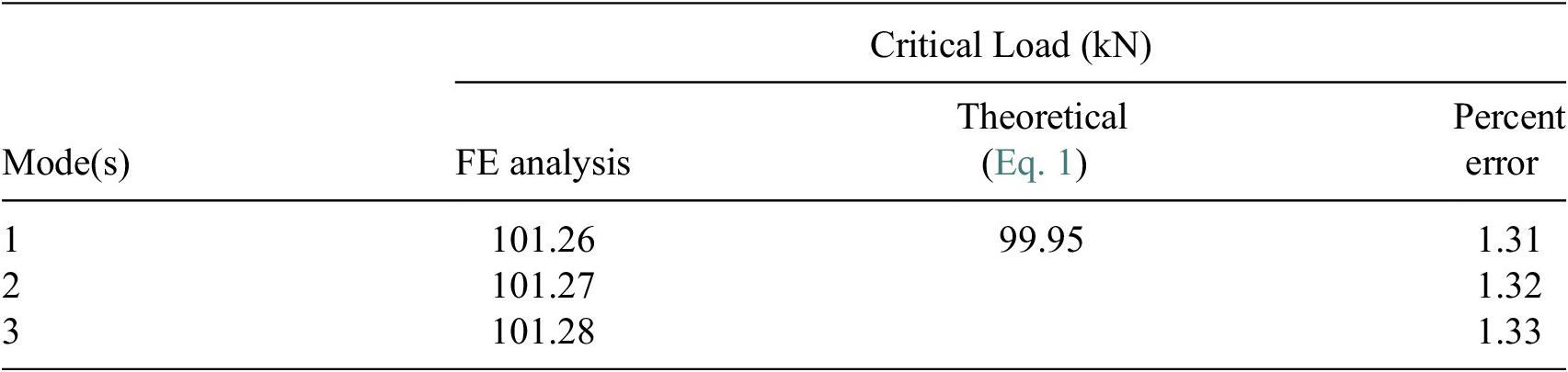
The closely spaced buckling modes obtained from linearized analysis are rarely realized in practice, as they interact through geometric nonlinearity and are strongly affected by geometric imperfections, causing instability to occur before the theoretical critical load is reached. To capture this realistic behavior, a nonlinear FE-based incremental iterative stability analysis is carried out using the Riks (arc-length) method (Riks, Reference Riks1978), which enables simultaneous load and displacement control and is well suited for tracing snap-through and snap-back responses typical of shell buckling. The procedure applies an initial reference load to compute the load proportionality factor (LPF), defined as the fraction of this load sustained at a given deformation level, with the maximum sustainable load obtained as the product of the initial load and the peak LPF. In this study, the lowest critical load from linear stability analysis is used as the reference load, and the resulting peak LPF is taken as the KDF. Figure A2 shows the typical load–displacement behavior of a perfect truncated conical shell (devoid of imperfections) with axial load.
Axial load–displacement behavior of perfect conical shell (without imperfection).

KDF is manifested by an abrupt reduction of approximately 5% in the fundamental (critical) load, primarily due to pre-buckling nonlinearity, closely spaced eigenmodes, and their nonlinear interactions. A more pronounced reduction in the critical load is observed when geometric imperfections are introduced. Figures A3a–d illustrate representative snapshots of the deformed shell configuration, denoted as points A, B, C, and D, corresponding to key stages along the load–displacement response as shown in Figure A2.
Deformed shell configurations corresponding to different fractions of the fundamental (critical) load, quantified by the LPF as (a) LPF = 0.04 at point A, (b) LPF = 0.80 at point B, (c) LPF = 0.95 at point C, and (d) LPF = 0.25 at point D.

A.2. Random geometric imperfections
Shell geometries inherently contain imperfections arising from manufacturing and construction deficiencies. Although advancements in fabrication techniques and stringent quality control measures have significantly reduced these deviations, they cannot be entirely eliminated. Such geometric imperfections lead to a further reduction in the critical buckling load. Traditionally, imperfections are assumed to be self-affine with respect to the corresponding buckling mode shapes (Riks, Reference Riks1978). In the present study, however, random imperfections are characterized using stochastic field representations (Majumder et al., Reference Majumder, Chakraborty and Mishra2023; Majumder and Mishra, Reference Majumder and Mishra2024). The geometric imperfections are modeled as two-dimensional, zero-mean, homogeneous Gaussian stochastic fields (Shinozuka and Deodatis, Reference Shinozuka and Deodatis1996), where the root mean square (r.m.s.) value defines the imperfection amplitude. For simplicity, the fields are assumed to be stationary, even though non-Gaussian imperfection patterns may also occur in practice (Papadopoulos et al., Reference Papadopoulos, Stefanou and Papadrakakis2009). Fluctuations in the geometric parameters are superimposed onto the ideal conical shell configuration to account for these imperfections (Papadopoulos and Lagaros, Reference Papadopoulos and Lagaros2009) as given in Equation A.1-A.2.
 $$ {R}_a\left(x,y\right)={\left({R}_a\right)}_0+{f}_1\left(x,y\right)\times {\left({R}_a\right)}_0{\displaystyle \begin{array}{ccccc}& (A.1)&; & t\left(x,y\right)={t}_0+{f}_2\left(x,y\right)\times {t}_0& (A.2)\end{array}} $$
where
 $ {\left({R}_a\right)}_0 $
and
$ {\left({R}_a\right)}_0 $
and
 $ {t}_0 $
are the average radius and thickness of the perfect cone and the random functions
$ {t}_0 $
are the average radius and thickness of the perfect cone and the random functions
 $ {f}_1\left(x,y\right) $
and
$ {f}_1\left(x,y\right) $
and
 $ {f}_2\left(x,y\right) $
represents random imperfections. Geometric imperfections alone are taken into account in this study, as they are recognized to have a more significant influence compared to other forms of imperfections (Majumder et al., Reference Majumder, Chakraborty and Mishra2023; Majumder and Mishra, Reference Majumder and Mishra2024).
$ {f}_2\left(x,y\right) $
represents random imperfections. Geometric imperfections alone are taken into account in this study, as they are recognized to have a more significant influence compared to other forms of imperfections (Majumder et al., Reference Majumder, Chakraborty and Mishra2023; Majumder and Mishra, Reference Majumder and Mishra2024).

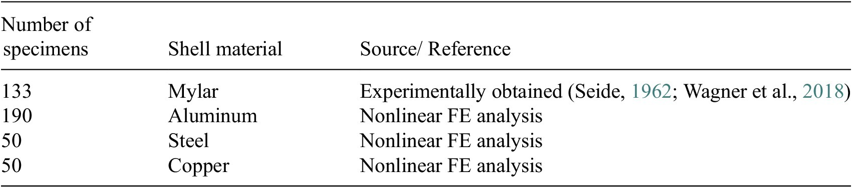
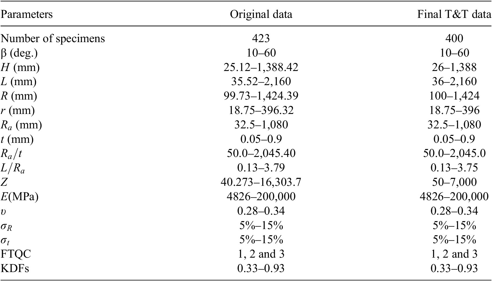

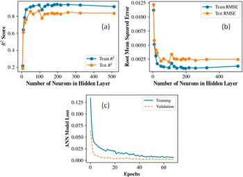


 Open access
Comments
No Comments have been published for this article.