





1 Introduction
Symmetric association measures—correlation,
$\chi ^{2}$
 , and the odds ratio (OR)—are well suited to dimensionality reduction and to discovering organizing latent factors, but they cannot distinguish
$A\rightarrow B$
, and the odds ratio (OR)—are well suited to dimensionality reduction and to discovering organizing latent factors, but they cannot distinguish
$A\rightarrow B$
 from
$B\rightarrow A$
from
$B\rightarrow A$
 . Standard regression of Y on X does not recover direction either: it presupposes it. Inferring direction from cross-sectional binary data is therefore intrinsically harder than inferring it from time-ordered data, and it is the situation that prevails in much of applied psychometrics.
Statistical implication analysis (SIA; Gras, Reference Gras1996; Gras et al., Reference Gras, Suzuki, Guillet and Spagnolo2008; Loevinger, Reference Loevinger1947, Reference Loevinger1948) reads asymmetry directly from the cells of a
$2\times 2$
 table by examining the relative scarcity of counter-examples
$(A,\bar {B})$
table by examining the relative scarcity of counter-examples
$(A,\bar {B})$
 . We adopt this stance. Existing implicative indices, however, have well-known limitations: they may saturate at their maximum without a clear implicative pattern, they ignore the contrapositive evidence
$(\bar {B}\rightarrow \bar {A})$
. We adopt this stance. Existing implicative indices, however, have well-known limitations: they may saturate at their maximum without a clear implicative pattern, they ignore the contrapositive evidence
$(\bar {B}\rightarrow \bar {A})$
 , they are not antisymmetric under direction reversal, and they do not aggregate naturally across many pairs into coherent network summaries.
This article proposes the iota index
$\iota $
 , which combines the main assertion with its contrapositive into a single asymmetric measure addressing these four points. Rather than warranting causal claims,
$\iota $
, which combines the main assertion with its contrapositive into a single asymmetric measure addressing these four points. Rather than warranting causal claims,
$\iota $
 flags pairs of events where the data permit a directional reading—statistical leverage points that downstream analyses (interventional designs, sensitivity analyses, and longitudinal follow-up) can confirm or rule out. In this sense, the index is hypothesis-generating: it identifies candidate
$A\rightarrow B$
flags pairs of events where the data permit a directional reading—statistical leverage points that downstream analyses (interventional designs, sensitivity analyses, and longitudinal follow-up) can confirm or rule out. In this sense, the index is hypothesis-generating: it identifies candidate
$A\rightarrow B$
 structure rather than certifying it. Comparable multivariate frameworks—Bayesian Networks in particular—cannot probabilistically distinguish networks that share an undirected skeleton (Verma & Pearl, Reference Verma and Pearl1990) and restrict the search space to acyclic structures, two limitations that
$\iota $
structure rather than certifying it. Comparable multivariate frameworks—Bayesian Networks in particular—cannot probabilistically distinguish networks that share an undirected skeleton (Verma & Pearl, Reference Verma and Pearl1990) and restrict the search space to acyclic structures, two limitations that
$\iota $
 -based graphs avoid.
To be clear about terminology, throughout this article, we use implication in the statistical and psychometric sense of an asymmetric dependency pattern between two binary events—the presence of one raising the probability of the other, with the same pattern showing in the contrapositive. This is the non-causal, asymmetric, predictive notion that logical implication itself encodes, and it is the pattern
$\iota $
 is designed to detect, in continuity with the SIA tradition. It should not be read as a causal statement in the counterfactual sense (Imbens & Rubin, Reference Imbens and Rubin2015; Pearl, Reference Pearl2009; Rubin, Reference Rubin1974), though it may serve as a descriptive starting point for further causal investigation under additional assumptions.
The article is organized as follows. Section 2 introduces the index, derives a significance test, and establishes its connection to the symmetric OR. Section 3 develops the link with item response theory—specifically the Rasch model—which grounds the dimensional reduction of implication graphs. The final section applies the framework to real developmental data.
2 The iota implication index
2.1 Construction
We define A and B as two binary variables that can take on values a and
$\bar {a}$
 , and b and
$\bar {b}$
, and b and
$\bar {b}$
 , respectively. We are interested in providing evidence of an implication relationship
$A\rightarrow B$
, respectively. We are interested in providing evidence of an implication relationship
$A\rightarrow B$
 , where the presence of A (
$A=a$
, where the presence of A (
$A=a$
 ) induces the presence of B (
$B=b$
) induces the presence of B (
$B=b$
 ). The available data are a joint frequency distribution, for which an underlying joint probability distribution is assumed. We will use symbols
$n_{ab}$
). The available data are a joint frequency distribution, for which an underlying joint probability distribution is assumed. We will use symbols
$n_{ab}$
 ,
$f_{ab}$
,
$f_{ab}$
 , and
$\pi _{ab}$
, and
$\pi _{ab}$
 to denote joint counts, relative frequencies, and population probabilities, respectively.
If a strict implication relationship
$A\rightarrow B$
 truly exists in the data, then there should be no exception that when A is present, B is also present, hence:

This is of course not realistic in a behavioral context, at least because the relational system constituted by A and B node events is likely not closed and many other causes are likely to interfere. But we shall take the conditional odds:

as an intensity measure of the logical implication relationship between both: Counter-examples should be rare compared to positive cases.
As is well known, a truly implicative relationship should also show itself through the contrapositive relationship
$\bar {B}\rightarrow \bar {A}$
 , so that we expect conditional odds:

to be large at the same time.
Finally, combining both expectations, we expect the following product (hereafter named the “iota” index):

to be large in the case of a statistical
$A\rightarrow B$
 implication relationship. Analogously, the reverse implication
$B\rightarrow A$
implication relationship. Analogously, the reverse implication
$B\rightarrow A$
 can be measured by

This index is asymmetric, in the sense that
$\iota _{A\rightarrow B}$
 and
$\iota _{B\rightarrow A}$
and
$\iota _{B\rightarrow A}$
 are unequal, in general. A final log transform will prove useful in the following sections, so that in practice the following form (“iota star”) will be used:

2.2 Basic properties and interpretation
In the form (1), the
$\iota ^{\ast}$
 index assesses the relative weights of concordance cases (simultaneous successes and simultaneous failures on both events) against counter-examples. A positive value shows evidence in favor of implication (concordant cases are more likely than counter-examples),
$\iota ^{\ast}=0$
index assesses the relative weights of concordance cases (simultaneous successes and simultaneous failures on both events) against counter-examples. A positive value shows evidence in favor of implication (concordant cases are more likely than counter-examples),
$\iota ^{\ast}=0$
 represents absence of implication or uncertainty (equal probabilities of concordant cases and counter-examples), and a negative value shows evidence against implication (exceptions are more probable than concordant cases). As will be demonstrated in the next section, under some conditions (but not in general), a negative value will also potentially be evidence of an inverse implicative relationship
$B\rightarrow A$
represents absence of implication or uncertainty (equal probabilities of concordant cases and counter-examples), and a negative value shows evidence against implication (exceptions are more probable than concordant cases). As will be demonstrated in the next section, under some conditions (but not in general), a negative value will also potentially be evidence of an inverse implicative relationship
$B\rightarrow A$
 .
.
In practice, available data on the association between two binary variables are joint frequencies in a
$2\times 2$
 table. Estimating the unknown joint probabilities by the observed joint frequencies leads to the following practical formula:

Four cases can be encountered in practice in the two-variable case: directed implication
$A\rightarrow B$
 , directed implication
$B\rightarrow A$
, directed implication
$B\rightarrow A$
 , symmetric implication
$A\rightleftharpoons B$
, symmetric implication
$A\rightleftharpoons B$
 , or no implication. These four cases are illustrated in Table 1.
Four examples of event asymmetric associations: (a) directed implication
$A\rightarrow B$
 , (b) directed implication
$B\rightarrow A$
, (b) directed implication
$B\rightarrow A$
 , (c) symmetric implication
$A\rightleftharpoons B$
, (c) symmetric implication
$A\rightleftharpoons B$
 , and (d) no implication

Table 1 Long description
The figure consists of four panels, each containing a two-by-two contingency table with row and column sums. All tables use variables a and bar a for rows, and b and bar b for columns.
Panel a, labeled directed implication A yields B. The header shows iota-hat star A yields B equals 2.197 and iota-hat star B yields A equals 0. Row a contains 0.30 and 0.10 with a sum of 0.40. Row bar a contains 0.30 and 0.30 with a sum of 0.60. Column sums are 0.60 and 0.40, totaling 1.00.
Panel b, labeled directed implication B yields A. The header shows iota-hat star A yields B equals 0 and iota-hat star B yields A equals 2.197. Row a contains 0.30 and 0.30 with a sum of 0.60. Row bar a contains 0.10 and 0.30 with a sum of 0.40. Column sums are 0.40 and 0.60, totaling 1.00.
Panel c, labeled symmetric implication. The header shows iota-hat star A yields B equals iota-hat star B yields A equals 2.197. Row a contains 0.375 and 0.125 with a sum of 0.5. Row bar a contains 0.125 and 0.375 with a sum of 0.5. Column sums are 0.5 and 0.5, totaling 1.00.
Panel d, labeled no implication. The header shows iota-hat star A yields B equals iota-hat star B yields A equals 0. Row a contains 0.25 and 0.25 with a sum of 0.5. Row bar a contains 0.25 and 0.25 with a sum of 0.5. Column sums are 0.5 and 0.5, totaling 1.00.
These four configurations span the qualitative space of dependence types and motivate why
$\iota ^{\ast}$
 must be reported as a pair. Cases (a) and (b) are mirror images: each shows a strong unidirectional implication (
$\hat {\iota }^{\ast}=2.197$
must be reported as a pair. Cases (a) and (b) are mirror images: each shows a strong unidirectional implication (
$\hat {\iota }^{\ast}=2.197$
 in the active direction,
$0$
in the active direction,
$0$
 in the other), so the asymmetry of the pair carries the directional information that the OR cannot resolve. Case (c) reveals that strong concordance lights up both directions simultaneously (
$\hat {\iota }_{A\rightarrow B}^{\ast}=\hat {\iota }_{B\rightarrow A}^{\ast}=2.197$
in the other), so the asymmetry of the pair carries the directional information that the OR cannot resolve. Case (c) reveals that strong concordance lights up both directions simultaneously (
$\hat {\iota }_{A\rightarrow B}^{\ast}=\hat {\iota }_{B\rightarrow A}^{\ast}=2.197$
 ), distinguishing symmetric implication from one-way implication. Case (d) anchors the zero. The key takeaway is that the pair
$(\iota _{A\rightarrow B}^{\ast},\iota _{B\rightarrow A}^{\ast})$
), distinguishing symmetric implication from one-way implication. Case (d) anchors the zero. The key takeaway is that the pair
$(\iota _{A\rightarrow B}^{\ast},\iota _{B\rightarrow A}^{\ast})$
 , rather than either component alone, characterizes the type of dependence: its asymmetry encodes direction, and its joint magnitude encodes strength.
2.3 A directional decomposition of the odds ratio
2.3.1 Relationship between the iota index and the odds ratio
The
$\iota $
 index reveals a fundamental connection to the well-established OR, providing a natural bridge between symmetric and asymmetric measures of association. The classical OR for a
$2\times 2$
index reveals a fundamental connection to the well-established OR, providing a natural bridge between symmetric and asymmetric measures of association. The classical OR for a
$2\times 2$
 contingency table is defined as

The iota index can be expressed as a directional modification of this OR:

Similarly, the reverse direction yields

This decomposition reveals that the
$\iota $
 index extends the OR by incorporating the discordance ratio
$\pi _{\bar {a}b}/\pi _{a\bar {b}}$
index extends the OR by incorporating the discordance ratio
$\pi _{\bar {a}b}/\pi _{a\bar {b}}$
 that specifically weights the relative prevalence of the two types of discordant observations. While the OR treats both discordant cells symmetrically, the iota index assigns differential importance based on the hypothesized direction of implication. This relationship between
$\iota _{A\rightarrow B}$
that specifically weights the relative prevalence of the two types of discordant observations. While the OR treats both discordant cells symmetrically, the iota index assigns differential importance based on the hypothesized direction of implication. This relationship between
$\iota _{A\rightarrow B}$
 and OR provides immediate interpretative value:
-
• When $\iota _{A\rightarrow B}>\text {OR}$
 : The directional correction factor exceeds unity, indicating that counterexamples to
$B\rightarrow A$
(i.e.,
$\pi _{\bar {a}b}$
) are more prevalent than counterexamples to
$A\rightarrow B$
(i.e.,
$\pi _{a\bar {b}}$
), supporting the
$A\rightarrow B$
direction.
: The directional correction factor exceeds unity, indicating that counterexamples to
$B\rightarrow A$
(i.e.,
$\pi _{\bar {a}b}$
) are more prevalent than counterexamples to
$A\rightarrow B$
(i.e.,
$\pi _{a\bar {b}}$
), supporting the
$A\rightarrow B$
direction. -
• When $\iota _{A\rightarrow B}<\text {OR}$
: The correction factor is less than unity, suggesting evidence against the
$A\rightarrow B$
direction. -
• When $\iota _{A\rightarrow B}\approx \text {OR}$
: The correction factor is close to unity, indicating that there is no clear directional preference in the association.


2.3.2 Reconstitution of the odds ratio
A remarkable property emerges when considering both directional indices simultaneously:

Therefore,

This elegant result demonstrates that the OR represents the geometric mean of the two directional iota indices. The symmetric association captured by the OR can thus be perfectly decomposed into two asymmetric components whose product preserves the original association strength. This shows that the well-known OR is a purely symmetric measure, while the
$\iota $
 index provides a decomposition into symmetric and asymmetric components. In psychometrics and cognitive diagnosis, where directionality is central, this decomposition offers an interpretable framework for distinguishing cumulative from reciprocal dependencies.
2.3.3 Properties on the logarithmic scale
The logarithmic transformation also yields interpretable relationships. Define the asymmetry parameter

On the log scale,

A noteworthy feature follows from the defining expression
$\iota ^{\ast}_{A\rightarrow B}=\log \pi _{ab}+\log \pi _{\bar a\bar b}-2\log \pi _{a\bar b}$
 :
$\iota ^{\ast}$
:
$\iota ^{\ast}$
 involves only three of the four cells of the
$2\times 2$
involves only three of the four cells of the
$2\times 2$
 table—the discordant cell
$\pi _{\bar a b}$
table—the discordant cell
$\pi _{\bar a b}$
 enters
$\Delta $
enters
$\Delta $
 and
$\log (\mathrm {OR})$
and
$\log (\mathrm {OR})$
 with opposite signs and cancels. This asymmetry in the roles of A and B is the formal counterpart of the directional-rule semantics: the rule “
$A \Rightarrow B$
with opposite signs and cancels. This asymmetry in the roles of A and B is the formal counterpart of the directional-rule semantics: the rule “
$A \Rightarrow B$
 ” is evaluated within the
$A=1$
” is evaluated within the
$A=1$
 row and along its contrapositive
$\bar B \Rightarrow \bar A$
row and along its contrapositive
$\bar B \Rightarrow \bar A$
 , not via the marginal frequency of B.
These expressions lead to two fundamental properties:
-
1. Sum property: The sum of the directional log-indices equals twice the log-OR:
(3) $$ \begin{align} \iota_{A\rightarrow B}^{\ast}+\iota_{B\rightarrow A}^{\ast}=2\log(\mathrm{OR}). \end{align} $$
-
2. Difference property: The difference isolates pure directionality:
(4) $$ \begin{align} \iota_{A\rightarrow B}^{\ast}-\iota_{B\rightarrow A}^{\ast}=2\Delta. \end{align} $$


2.4 Inference for directed dependence
2.4.1 Decomposition into association and asymmetry
The decompositions

or, on the log scale,

make explicit that
$\iota $
 combines two conceptually distinct sources of information: (i) the presence of statistical association between A and B, captured by the OR and (ii) directional imbalance among discordant observations, captured by the ratio
$\pi _{\bar a b}/\pi _{a\bar b}$
combines two conceptually distinct sources of information: (i) the presence of statistical association between A and B, captured by the OR and (ii) directional imbalance among discordant observations, captured by the ratio
$\pi _{\bar a b}/\pi _{a\bar b}$
 .
.
Note that, in the case of independence, the OR is one, and the
$\iota $
 index for
$A \rightarrow B$
index for
$A \rightarrow B$
 is
is

which depends only on the marginal distributions of A and B. In this situation,
$\iota $
 no longer reflects a relational property between the two variables, but merely encodes marginal heterogeneity. Consequently, directional imbalance in the absence of association is not substantively interpretable as evidence of directed dependence.
This observation motivates an inferential strategy in which the existence of an association link is treated as a prerequisite for the interpretation of directional asymmetry. Such a strategy mirrors standard practice in other areas of statistics, such as contrast testing in ANOVA, where contrasts are typically interpreted only conditional on a statistically significant omnibus effect. Analogously, in the present framework, directional asymmetry is interpreted only when there is evidence of association, as indicated by a non-unit OR.
These two steps, and their integration into a unified testing procedure, are described in the three following sections.
2.4.2 Test of association (odds ratio)
For an unordered pair
$(A,B)$
 of events, we first test the null hypothesis of no positive association:

using a one-sided Wald test for the log-OR computed from the
$2\times 2$
 contingency table. A one-sided test is appropriate here because implication relationships require positive association: whatever the direction of implication (
$A \to B$
contingency table. A one-sided test is appropriate here because implication relationships require positive association: whatever the direction of implication (
$A \to B$
 or
$B \to A$
or
$B \to A$
 ), success at one item should make success at the other more likely, implying
$\mathrm {OR}> 1$
), success at one item should make success at the other more likely, implying
$\mathrm {OR}> 1$
 . Negative associations would indicate a qualitatively different relationship (e.g., mutual exclusivity) that falls outside the scope of implication analysis.
Define the OR parameter

A natural plug-in estimator is

Under an independent Poisson sampling scheme, using
$\operatorname {Var}(\log n_{ij})= 1/\mu _{ij}$
 and
$\hat {\mu }_{ij}= n_{ij}$
and
$\hat {\mu }_{ij}= n_{ij}$
 , its asymptotic variance is obtained as

Test
$H^{\text {assoc}}_{0}$
 with
with

and
$p^{\text {assoc}}=1-\Phi (Z_{\text {OR}})$
 the corresponding one-sided p-value.
2.4.3 Test of asymmetry among discordant observations
Conditional on association, directionality is assessed through the imbalance of discordant cells. Specifically, we test

using a two-sided Wald test based on the estimated log ratio of discordant probabilities.
This test is direction-neutral: rejection indicates the presence of asymmetric dependence, while the sign of the statistic determines the direction of implication.
Define the asymmetry parameter

Assuming independent Poisson counts, its asymptotic variance is obtained as

We test
$H^{\text {asym}}:\ \Delta =0$
 using
using

and
$p^{\text {asym}}=2\bigl (1-\Phi (|Z_{\text {asym}}|)\bigr )$
 the corresponding two-sided p-value.
Direction, if any, is then given by
$\operatorname {sign}(\widehat {\Delta })$
 , with
$\widehat {\Delta }>0$
, with
$\widehat {\Delta }>0$
 (or
$n_{\bar {a}b}>n_{a\bar {b}}$
(or
$n_{\bar {a}b}>n_{a\bar {b}}$
 ) suggesting an
$A\rightarrow B$
) suggesting an
$A\rightarrow B$
 direction, and
$\widehat {\Delta }<0$
direction, and
$\widehat {\Delta }<0$
 (or
$n_{\bar {a}b}<n_{a\bar {b}}$
(or
$n_{\bar {a}b}<n_{a\bar {b}}$
 ) suggesting a
$B\rightarrow A$
) suggesting a
$B\rightarrow A$
 direction.
2.4.4 Joint inference for directed dependence
To formalize the requirement that both positive association and asymmetry be present for a directed relation to be interpretable, we define the composite null hypothesis

that is, either no positive association or no asymmetry.
The alternative hypothesis corresponds to the simultaneous presence of positive association and asymmetry. A conservative p-value for this intersection alternative is given by

which is valid by standard union–intersection testing arguments: the null is rejected only if both component tests provide evidence against their respective null hypotheses.
2.4.5 Illustration
As an illustration, we consider the data reported by Lecoutre and Charron (Reference Lecoutre and Charron2000) on the development of number knowledge among
$N = 165$
 children (Table 2). The study focuses on fraction calculation and interpretation tasks of two types: (i) part-to-part items (e.g., “there is a 3-to-4 ratio of oranges to apples in this basket of 28 fruits”) and (ii) part-to-whole items (e.g., “3 out of 6 slices have been eaten”). In the literature on numerical cognition, part-to-part fractions are generally considered more difficult than part-to-whole fractions.
Lecoutre and Charron’s (Reference Lecoutre and Charron2000) data on fraction mastery

Table 2 Long description
The table cross-tabulates two variables: Part-to-part mastery (rows) and Part-to-whole mastery (columns).
Column Headers:
* Column 1: Empty top-left cell.
* Column 2: Part-to-whole success (b).
* Column 3: Part-to-whole failure (b-bar).
* Column 4: Sums.
Row 1 (Part-to-part success (a)):
* Success in both (n sub a b): 36.
* Part-to-part success but part-to-whole failure (n sub a b-bar): 3.
* Total part-to-part success (n sub a): 39.
Row 2 (Part-to-part failure (a-bar)):
* Part-to-part failure but part-to-whole success (n sub a-bar b): 36.
* Failure in both (n sub a-bar b-bar): 90.
* Total part-to-part failure (n sub a-bar): 126.
Row 3 (Sums):
* Total part-to-whole success (n sub b): 72.
* Total part-to-whole failure (n sub b-bar): 93.
* Grand total (N): 165.
Let A denote success on the part-to-part item and B success on the part-to-whole item. The joint response counts are given in Table 2.
The OR is estimated as

yielding
$\log (\widehat {\mathrm {OR}}_{AB})=\log (30)\approx 3.40$
 .
.
Under the independent-Poisson sampling scheme, the estimated variance of
$\log (\widehat {\mathrm {OR}}_{AB})$
 is
$1/36+1/90+1/3+1/36=0.40$
is
$1/36+1/90+1/3+1/36=0.40$
 , so that the Wald statistic is
$Z_{\mathrm {OR}}=3.40/\sqrt {0.40}\approx 5.38$
, so that the Wald statistic is
$Z_{\mathrm {OR}}=3.40/\sqrt {0.40}\approx 5.38$
 , corresponding to a one-sided p-value
$p^{\mathrm {assoc}}_{AB}\approx 3.7\times 10^{-8}$
, corresponding to a one-sided p-value
$p^{\mathrm {assoc}}_{AB}\approx 3.7\times 10^{-8}$
 . This result provides strong evidence of positive association between the two items.
Directional asymmetry is assessed through the imbalance of discordant outcomes. The estimated asymmetry parameter is
$\widehat {\Delta }_{AB}=\log (36/3)=\log (12)\approx 2.48$
 , with estimated variance
$1/36+1/3\approx 0.36$
, with estimated variance
$1/36+1/3\approx 0.36$
 , leading to the Wald statistic
$Z_{\mathrm {asym}}=2.48/\sqrt {0.36}\approx 4.14$
, leading to the Wald statistic
$Z_{\mathrm {asym}}=2.48/\sqrt {0.36}\approx 4.14$
 and a two-sided p-value
$p^{\mathrm {asym}}_{AB}\approx 3.5\times 10^{-5}$
and a two-sided p-value
$p^{\mathrm {asym}}_{AB}\approx 3.5\times 10^{-5}$
 .
.
The overall implication index is then obtained as the sum of both components:
$\widehat {\iota }^{\ast}_{A\rightarrow B} = \log (\widehat {\mathrm {OR}}_{AB}) + \widehat {\Delta }_{AB} = 3.40 + 2.48 = 5.88$
 .
.
Following the inferential strategy proposed above, directional dependence is assessed through the composite null hypothesis
$H^{\mathrm {dir}}_{AB}:\ \log (\mathrm {OR}_{AB}) \leq 0\ \text {or}\ \log (\pi _{\bar a b}/\pi _{a\bar b})=0$
 , with a conservative p-value given by
$p^{\mathrm {dir}}_{AB}=\max (p^{\mathrm {assoc}}_{AB},\,p^{\mathrm {asym}}_{AB})\approx 3.5\times 10^{-5}$
, with a conservative p-value given by
$p^{\mathrm {dir}}_{AB}=\max (p^{\mathrm {assoc}}_{AB},\,p^{\mathrm {asym}}_{AB})\approx 3.5\times 10^{-5}$
 .
.
The sign of
$\widehat {\Delta }_{AB}>0$
 indicates that discordant responses are dominated by the pattern
$(\bar a,b)$
indicates that discordant responses are dominated by the pattern
$(\bar a,b)$
 , corresponding to success on the part-to-whole item without success on the part-to-part item. Equivalently, success on the more difficult part-to-part task is almost always accompanied by success on the easier part-to-whole task.
Taken together, these results indicate a strong asymmetric dependence between the two items, consistent with a cumulative structure in fraction knowledge. Importantly, this conclusion is drawn only after establishing the presence of association between the tasks, thereby avoiding the conflation of directional imbalance with marginal difficulty effects alone.
The decomposition into an asymmetry and an association component suggests a natural two-dimensional representation for pairs of binary variables. By plotting the directional asymmetry and
$\log (\widehat {\mathrm {OR}})$
 estimates on the first and second axis, respectively, one obtains an immediate visual representation where the Euclidean distance from the origin relates to the overall dependency strength, but: (i) points on the x-axis indicate directional preference and (ii) vertical displacement from the x-axis represents purely symmetric associations (OR). This is illustrated in Figure 1 for Lecoutre and Charron’s (Reference Lecoutre and Charron2000) data discussed above. This representation provides an intuitive framework for exploring asymmetric relationships, where the familiar concept of association strength (through the OR) is augmented with directional information.
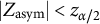
Association–directionality plot for Lecoutre and Charron’s (Reference Lecoutre and Charron2000) data on part-to-part and part-to-whole fractions. Implication appears to be in the upper right quadrant, that is, in the part-to-part
$\rightarrow $
 part-to-whole (
$A\rightarrow B$
part-to-whole (
$A\rightarrow B$
 ) direction. The shaded bands indicate non-significance regions for association (horizontal,
$|Z_{\mathrm {OR}}| < z_{\alpha }$
) direction. The shaded bands indicate non-significance regions for association (horizontal,
$|Z_{\mathrm {OR}}| < z_{\alpha }$
 ) and directionality (vertical,
$|Z_{\mathrm {asym}}| < z_{\alpha /2}$
) and directionality (vertical,
$|Z_{\mathrm {asym}}| < z_{\alpha /2}$
 ), computed from the asymptotic standard errors of
$\log (\widehat {\mathrm {OR}})$
), computed from the asymptotic standard errors of
$\log (\widehat {\mathrm {OR}})$
 and
$\widehat {\Delta }$
and
$\widehat {\Delta }$
 , respectively.

2.4.6 Conditional directed dependence (adjustment for observed covariates)
The inferential framework described above can be extended in a straightforward manner to account for observed covariates. Let
$C\in \{0,1\}$
 denote a binary covariate and consider the conditional joint distributions of A and B within strata
$C=c$
denote a binary covariate and consider the conditional joint distributions of A and B within strata
$C=c$
 .
.
For each stratum c, we define the conditional implication index

which admits the same decomposition as in the marginal case,

or, on the log scale,

Inference is conducted on both components within each stratum using the same two-step strategy as in the marginal case: a one-sided Wald test for positive association, followed by a two-sided Wald test for asymmetry. The corresponding pooled formula and inferential procedure are described in Appendix A.
3 A natural connection to the Rasch model
In this section, we consider the particular case where events are responses to success–failure tests, and the underlying structure is a one-parameter Rasch model. We first note that, as a probabilistic formulation of a Guttman scale, the Rasch model is conceptually an implicative model: Success on a given item statistically implies success on easier items, when the reverse is highly unlikely. Consider the response variables
$X_{1}$
 and
$X_{2}$
and
$X_{2}$
 on two items following a Rasch response model, with difficulty parameters
$\delta _{1}$
on two items following a Rasch response model, with difficulty parameters
$\delta _{1}$
 and
$\delta _{2}$
and
$\delta _{2}$
 .
.
Now, denoting variable values (success and failure) by 1 and 0, the marginal success probabilities for item
$X_{j}$
 under the Rasch are defined as

Assuming conditional independence among responses for a given
$\theta $
 , the theoretical joint distribution on both items is given by

with
$\gamma =\left [1+\exp (\theta -\delta _{1})\right ]\left [1+\exp (\theta -\delta _{2})\right ]$
 the normalizing constant.
Within this particular model, we have the conditional odds given
$\theta $
 :
:

and the
$\iota $
 index becomes

which is independent of
$\theta $
 .
.
This is a very simple and remarkable result: This implication measure is a simple increasing function of the inter-item distance along the latent dimension, which goes to infinity as
$\delta _{1}$
 is large with respect to
$\delta _{2}$
is large with respect to
$\delta _{2}$
 (success on a difficult item implies success on an easier item), tends to zero if
$X_{1}$
(success on a difficult item implies success on an easier item), tends to zero if
$X_{1}$
 is easier than
$X_{2}$
is easier than
$X_{2}$
 , and equals 1 when both items are of similar difficulty (i.e., success on any one of them does not help predict success on the other).
3.1 Properties under the Rasch
Four properties of the
$\iota ^{\ast}$
 index under the Rasch model are noteworthy:
-
1. Symmetry: The reversed implication $X_{2}\rightarrow X_{1}$
is measured using $$ \begin{align*} o_{.1} & = \frac{\pi_{ab}}{\pi_{\bar{a}b}}=\exp(\theta-\delta_{1}),\\ o_{0.} & = \frac{\pi_{\bar{a}\bar{b}}}{\pi_{\bar{a}b}}=\exp\left[-(\theta-\delta_{2})\right], \end{align*} $$and the reversed $\iota _{X_{2}\rightarrow X_{1}}$
index reads $$\begin{align*}\iota_{X_{2}\rightarrow X_{1}{\mid\theta}}=o_{.1}\times o_{0.}=\exp(\delta_{2}-\delta_{1})=\frac{1}{\iota}. \end{align*}$$Log transforming the $\iota $
index, we note that $$\begin{align*}\iota_{X_{1}\rightarrow X_{2}{\mid\theta}}^{\ast}=\delta_{1}-\delta_{2}=-\iota_{X_{2}\rightarrow X_{1}{\mid\theta}}^{\ast}. \end{align*}$$Provided a Rasch model holds, the $\iota ^{\ast}$
index is a signed measure of implication: It is zero when there is no implication, positive when
$(X_{1}=1)\rightarrow (X_{2}=1)$
, and negative when the reverse implication holds. The measure is symmetric in absolute value, in the sense that
$\left |\iota _{X_{1}\rightarrow X_{2}{\mid \theta }}^{\ast}\right |=\left |\iota _{X_{2}\rightarrow X_{1}{\mid \theta }}^{\ast}\right |$
, a negative value of the index meaning “is implied.”
-
2. Additivity: Under the restrictive conditions of a Rasch model, it may also be seen that $\iota ^*$
measures are additive: (8) $$ \begin{align} \iota_{X_{1}\rightarrow X_{3}{\mid\theta}}^{\ast}=\delta_{1}-\delta_{3}=(\delta_{1}-\delta_{2})+(\delta_{2}-\delta_{3})=\iota_{X_{1}\rightarrow X_{2}{\mid\theta}}^{\ast}+\iota_{X_{2}\rightarrow X_{3}{\mid\theta,}}^{\ast} \end{align} $$which can be interpreted as a transitivity property on implication relationships.
-
3. Constrained implication: From (7), we see that if $\delta _{1}\ge \delta _{2}$
, we have
$\iota \ge 1$
, so that both components in the index cannot fall below 1. -
4. Marginal asymmetry identity: The three properties above are derived conditionally on $\theta $
and do not in general carry over verbatim to the population level. The asymmetry component
$\Delta _{12}=\log (\pi _{\bar a b}/\pi _{a\bar b})$
of the
$\iota ^{\ast}$
decomposition, however, does retain a clean Rasch identity in the marginal case: under the Rasch model, (9) $$ \begin{align} \Delta_{12}=\delta_{1}-\delta_{2} \end{align} $$even when $\Delta _{12}$
is computed from population-level probabilities with variable
$\theta $
. To see this, note that under conditional independence, $$ \begin{align*} P(X_{1}=1\mid X_{1}+X_{2}=1,\theta) & =\frac{P(X_{1}=1,X_{2}=0\mid\theta)}{P(X_{1}=1,X_{2}=0\mid\theta)+P(X_{1}=0,X_{2}=1\mid\theta)}\\ & =\frac{1}{1+\exp(\delta_{1}-\delta_{2})}, \end{align*} $$which does not depend on $\theta $
. Taking the expectation over
$\theta $
therefore leaves the right-hand side unchanged, so
$P(X_{1}=1\mid X_{1}+X_{2}=1)=1/[1+\exp (\delta _{1}-\delta _{2})]$
at the population level, and hence
$\pi _{\bar a b}/\pi _{a\bar b}=\exp (\delta _{1}-\delta _{2})$
.











These properties characterize a Rasch scale as a pure, parameterized, implication structure: the first three describe its behavior within homogeneous
$\theta $
 subpopulations, while the marginal asymmetry identity (9) carries the structure to the population level and is what justifies the multidimensional scaling (MDS) approach developed below at the marginal level.
3.2 A multidimensional scaling approach to Rasch analysis
An important property of the
$\iota $
 index in the Rasch case is its independence with respect to any aptitude
$\theta $
index in the Rasch case is its independence with respect to any aptitude
$\theta $
 parameter. All pairs of observed responses
$(x_{i1},x_{i2})$
parameter. All pairs of observed responses
$(x_{i1},x_{i2})$
 on two given items for all persons (
$i=1,\ldots ,N$
on two given items for all persons (
$i=1,\ldots ,N$
 ) will bring an equivalent information in its computation. Assuming a marginal Poisson model on the joint observed counts, joint relative frequencies may be directly used to construct an empirical implication index:

provided
$f_{a\bar {b}}\neq 0$
 . If a Rasch model truly holds, an estimate of the (unsigned) inter-item distance is given by

Of course, this limits us to the cases where all counts are non-null, but note that in the case
$n_{a\bar {b}}=0$
 , an independent estimator of the same distance under the Rasch model is also provided by

which can be used as a replacement if available.
If such a distance estimate is computed for two items
$I_{1}$
 and
$I_{2}$
and
$I_{2}$
 , and then on
$I_{2}$
, and then on
$I_{2}$
 and a third item
$I_{3}$
and a third item
$I_{3}$
 , then if the Rasch model holds and from (8), we should approximately have the classical additive property:

This suggests an MDS approach to estimating item difficulties in a Rasch model. The matrix of all pairwise (unsigned) distance estimates from Equation (10) may be submitted to a classical metric MDS procedure. If all items respect a Rasch response model, then all the corresponding points should be approximately aligned in the MDS space, and a one-dimensional solution should show an acceptable fit.
We note that this property is preserved under conditioning on observed covariates (Formula (6)): when a Rasch model holds within each stratum, the conditional iota retains its interpretation as inter-item distance along the latent dimension. The dimensional analysis described above can then be applied to pooled or stratum-specific iota matrices, depending on whether homogeneity holds across strata.
This alignment property sets the stage for an integrated network/dimensional representation of dependency relationships, hereafter named as dimensional implication graph (DIG), schematically illustrated in Figure 2 for seven variables. Although various pairwise or MDS approaches for estimating Rasch model parameters, based on different proximity measures, have already been proposed in the literature (Choppin, Reference Choppin1982; Davison & Wood, Reference Davison and Wood1983; Garner & Engelhard, Reference Garner and Engelhard2009; Wright & Masters, Reference Wright and Masters1982), this one has the advantage of having a clear implicative interpretation.
Schematic illustration of a dimensional implication graph in the canonical Rasch case for seven variables. The figure deliberately combines two layers of information that, separately, are familiar but, together, are not: a directed graph structure (success on a more difficult item implies probable success on an easier item, but not the other way around), overlaid on a metrically meaningful spatial layout in which inter-node distances reflect latent difficulty differences
$|\delta _i-\delta _j|$
 .
.

Figure 2 Long description
The diagram is organized into three vertical layers.
At the top is the Implication layer, consisting of multiple gray curved arrows. These arrows originate from items on the right and point toward items on the left, indicating that success on a higher-indexed item implies success on lower-indexed items.
The middle layer, labeled Items, contains seven oval nodes arranged in a horizontal line from left to right, labeled X sub 1, X sub 2, X sub 3, X sub 4, X sub 5, X sub 6, and X sub 7.
The bottom layer, labeled Difficulties, is a horizontal metric scale. It features a thin line with vertical tick marks aligned directly under each item node. These tick marks are labeled with the Greek letter delta and a corresponding subscript number from 1 to 7. The spatial distance between these delta markers varies, representing the absolute difference in latent difficulty between the items. For example, the distance between delta sub 1 and delta sub 2 is larger than the distance between delta sub 6 and delta sub 7.
We note in passing that, under a strictly unidimensional Rasch structure, the marginal asymmetry identity
$\Delta _{ij}=\delta _i-\delta _j$
 implies that
$\delta _i$
implies that
$\delta _i$
 could equivalently be estimated by averaging the signed
$\hat \Delta _{ij}$
could equivalently be estimated by averaging the signed
$\hat \Delta _{ij}$
 over j, recovering
$\delta _i$
over j, recovering
$\delta _i$
 up to a translation constant. The MDS approach adopted here is preferred because the proportion of variance explained on the first MDS coordinate provides an internal goodness-of-fit indicator for the unidimensionality assumption itself: when the data are well described by a single Rasch scale, the first eigenvalue dominates; when they are not, the dropoff is shallow, alerting the analyst to escalate to the multiple-scale analysis developed in the next section. The simpler averaging estimator returns a value for every item regardless and cannot diagnose its own breakdown.
3.3 Separation of multiple Rasch scales
We examine in this section how a mixture of Rasch scales can be geometrically separated, by using proper association measures derived from the
$\iota ^{\ast}$
 index. Throughout this section, the model assumes one latent variable
$\theta _k$
index. Throughout this section, the model assumes one latent variable
$\theta _k$
 per Rasch scale (two in the derivations below); the population parameters
$(\mu _k,\ \sigma _k^{2})$
per Rasch scale (two in the derivations below); the population parameters
$(\mu _k,\ \sigma _k^{2})$
 and the inter-scale covariance
$\sigma _{12}$
and the inter-scale covariance
$\sigma _{12}$
 are kept explicit because they govern the empirical separability properties exploited by the methodology.
3.3.1 The expected structure
In the case of items drawn from two Rasch scales with correlated traits, the joint probabilities for a given respondent and the pair
$(\theta _{1},\ \theta _{2})$
 of corresponding aptitudes are given by

with
$\gamma _{12}=\left [1+\exp (\theta _{1}-\delta _{1})\right ]\left [1+\exp (\theta _{2}-\delta _{2})\right ]$
 the normalizing constant.
The conditional implication intensity, for a given pair
$(\theta _{1},\theta _{2})$
 , is
, is

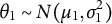
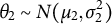
Under the common assumption of Gaussian distributions for person parameters, that is,
$\theta _{1}\sim N(\mu _{1},\sigma _{1}^{2})$
 and
$\theta _{2}\sim N(\mu _{2},\sigma _{2}^{2})$
and
$\theta _{2}\sim N(\mu _{2},\sigma _{2}^{2})$
 , we have
$\theta _{2}-\theta _{1}\sim N(\mu _{2}-\mu _{1},\sigma _{1}^{2}+\sigma _{2}^{2}-2\sigma _{12})$
, we have
$\theta _{2}-\theta _{1}\sim N(\mu _{2}-\mu _{1},\sigma _{1}^{2}+\sigma _{2}^{2}-2\sigma _{12})$
 , where
$\sigma _{12}$
, where
$\sigma _{12}$
 denotes the covariance between both latent scores. The variable
$Z=\exp (\theta _{2}-\theta _{1})$
denotes the covariance between both latent scores. The variable
$Z=\exp (\theta _{2}-\theta _{1})$
 is by definition log-normally distributed with parameters
$\mu _{2}-\mu _{1}$
is by definition log-normally distributed with parameters
$\mu _{2}-\mu _{1}$
 and
$\frac {\sigma _{1}^{2}+\sigma _{2}^{2}-2\sigma _{12}}{2}$
and
$\frac {\sigma _{1}^{2}+\sigma _{2}^{2}-2\sigma _{12}}{2}$
 . From the properties of the lognormal, the corresponding expectation is
$E(Z)=\exp \left (\mu _{2}-\mu _{1}+\tfrac {\sigma _{1}^{2}+\sigma _{2}^{2}}{2}-\sigma _{12}\right )$
. From the properties of the lognormal, the corresponding expectation is
$E(Z)=\exp \left (\mu _{2}-\mu _{1}+\tfrac {\sigma _{1}^{2}+\sigma _{2}^{2}}{2}-\sigma _{12}\right )$
 .
.
Finally, we have, marginally,

and on the log-scale,

This last expression helps clarify that, in the presence of two Rasch scales, the
$\iota ^*$
 index decomposes into two components: a directional component, reflecting item and scale shifts, and a symmetric component that reflects the latent covariance structure.
Both components can be separated. Writing the symmetric counterpart of (11) gives

Analogously to Equations (3) and (4), (half) summing and differencing both expressions then yield the pure association and directionality quantities:

We note that only the A component depends upon the latent ability.
3.3.2 Extraction from empirical data
From Equations (3) and (4), the half-sum and half-difference within a pair of empirical
$\iota ^*$
 are interpretable as a difficulty difference (
$\hat {\Delta }$
are interpretable as a difficulty difference (
$\hat {\Delta }$
 ) and an association strength (
$\log (\widehat {\mathrm {OR}})$
) and an association strength (
$\log (\widehat {\mathrm {OR}})$
 ). Given the marginal nature of observed counts, some attenuation is expected on the association component, which depends on the latent ability variance. It is shown in Appendix B that, under the Rasch model, the expected marginal log-OR for any item pair within a scale is approximately constant, and given by the special case of Formula (B.1) with
$a_i=a_j=1$
). Given the marginal nature of observed counts, some attenuation is expected on the association component, which depends on the latent ability variance. It is shown in Appendix B that, under the Rasch model, the expected marginal log-OR for any item pair within a scale is approximately constant, and given by the special case of Formula (B.1) with
$a_i=a_j=1$
 :
:

where
$\sigma ^2$
 is the latent ability variance. In the multiple Rasch scale case, the expected marginal log-OR also depends upon the latent correlation between the scales and may be approximated by (Formula (B.2))

Figure 3 illustrates the quality of these approximations, in a
$(\hat {\Delta },\log (\widehat {\mathrm {OR}}))$
 representation of a simulated dataset that mixes two 8-item Rasch scales, equally spaced in
$[-2;2]$
representation of a simulated dataset that mixes two 8-item Rasch scales, equally spaced in
$[-2;2]$
 , with two levels of latent correlation (
$\rho =0$
, with two levels of latent correlation (
$\rho =0$
 and
$\rho =0.5$
and
$\rho =0.5$
 ). Within-scale pairs—which share a common latent trait—exhibit elevated
$\log (\widehat {\mathrm {OR}})$
). Within-scale pairs—which share a common latent trait—exhibit elevated
$\log (\widehat {\mathrm {OR}})$
 due to the positive marginal association induced by marginalization over
$\theta $
due to the positive marginal association induced by marginalization over
$\theta $
 . In contrast, cross-scale pairs under independence show near-zero
$\log (\widehat {\mathrm {OR}})$
. In contrast, cross-scale pairs under independence show near-zero
$\log (\widehat {\mathrm {OR}})$
 (see gray triangles aligned along the x-axis in panels (a) and (c)). But these cross-scale association values increase with trait correlation, reducing the difference with the within log-OR values (panels (b) and (d)) and thereby degrading separability. Expected within- and between-scale log-OR levels, computed from these approximations, are plotted as horizontal gray lines on the figure.
Directionality (
$\hat {\Delta }$
 ) versus Association (
$\log (\widehat {\mathrm {OR}})$
) versus Association (
$\log (\widehat {\mathrm {OR}})$
 ) for 120 item pairs from two simulated 8-item Rasch scales, varying latent correlation (
$\rho =0,0.5$
) for 120 item pairs from two simulated 8-item Rasch scales, varying latent correlation (
$\rho =0,0.5$
 ) and variance (
$\sigma _1=1,2$
) and variance (
$\sigma _1=1,2$
 ). The constant vertical offset between within-scale and between-scale pairs reflects the difference in marginal association (augmented by variance and diminished by correlation). The approximately constant expected marginal within- and between-scale log-OR levels (obtained from the within- and between-scale approximations of Appendix B) are plotted as gray horizontal lines.

Figure 3 Long description
A four-panel scatter plot grid labeled a through d. Each panel has a horizontal x-axis labeled with the symbol phi ranging from negative 4 to 4 and a vertical y-axis labeled log O R ranging from negative 0.5 to 2.5. Three data series are present in each panel: Within scale 1 represented by blue circles, Within scale 2 represented by red squares, and Between scales represented by gray triangles.
* Panel a: sigma sub 1 equals 1, sigma sub 2 equals 1, rho equals 0. Blue circles and red squares are clustered together between log O R 0.5 and 1.0. Gray triangles are clustered lower, around log O R 0.0.
* Panel b: sigma sub 1 equals 1, sigma sub 2 equals 1, rho equals 0.5. The blue and red clusters remain between 0.5 and 1.0, but the gray triangles shift upward toward log O R 0.5, narrowing the gap between series.
* Panel c: sigma sub 1 equals 2, sigma sub 2 equals 1, rho equals 0. Blue circles shift significantly upward to cluster around log O R 1.8. Red squares remain around 0.7, and gray triangles remain around 0.0.
* Panel d: sigma sub 1 equals 2, sigma sub 2 equals 1, rho equals 0.5. Blue circles remain high at 1.8. Red squares and gray triangles both shift slightly upward, with gray triangles now overlapping the lower range of the red squares around log O R 0.6.
In all panels, gray dashed horizontal lines indicate the expected marginal levels for each scale grouping.
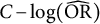
Individual item layout reconstructed from separate unidimensional MDS analyses i) on the
$|\hat {\Delta }|$
 matrix (x-axis) and ii) on the
$C-\log (\widehat {\mathrm {OR}})$
matrix (x-axis) and ii) on the
$C-\log (\widehat {\mathrm {OR}})$
 matrix (y-axis), for the simulated data of Figure 3. Horizontal dashed lines illustrate a separation obtained through k-means clustering. Scale separability increases with difference in latent variance and decreases with latent correlation. In the absence of latent correlation (panels a and c), no between-scale links appear; in the correlated case (panels b and d), undirected between-scale links (black) tend to connect items of similar difficulty across the two scales, while directed links (dark gray) arise when a difficulty difference is also present.

Figure 4 Long description
The four panels are arranged in a two-by-two grid, labeled a through d. Each panel shares the same axes: the x-axis represents Difficulty ranging from negative 2 to 2, and the y-axis represents Associative locations ranging from negative 2 to 2.
* Panel a (top-left): Sigma sub 1 equals 1, sigma sub 2 equals 1, rho equals 0. Items i 1 through i 8 form a horizontal cluster at y equals 0.5, connected by light blue curved links. Items i 9 through i 16 form a horizontal cluster at y equals negative 0.5, connected by dark red curved links. No links exist between the two clusters.
* Panel b (top-right): Sigma sub 1 equals 1, sigma sub 2 equals 1, rho equals 0.5. The item clusters are positioned similarly to panel a. However, black symmetric links and dark gray directed links now connect items between the top and bottom clusters, primarily between items of similar difficulty.
* Panel c (bottom-left): Sigma sub 1 equals 2, sigma sub 2 equals 1, rho equals 0. The top cluster (i 1 to i 8) is shifted upward to y equals 1.2, while the bottom cluster (i 9 to i 16) is shifted downward to y equals negative 1.2. There are no links between the clusters.
* Panel d (bottom-right): Sigma sub 1 equals 2, sigma sub 2 equals 1, rho equals 0.5. The clusters are vertically separated as in panel c. Dense networks of dark gray directed links connect the two clusters, showing a high degree of cross-scale interaction despite the increased vertical distance.
A legend in the top-right of panel b identifies the link types: light blue for Within scale A, dark red for Within scale B, black for Between symmetric, and dark gray for Between directed.
For graph plotting, an optimal item layout may be obtained by extracting individual item locations from these two sets of item pair relationships. This is obtained through two separate unidimensional MDS on the properly transformed
$\hat {\Delta }$
 and
$\log (\widehat {\mathrm {OR}})$
and
$\log (\widehat {\mathrm {OR}})$
 matrices. On the
$\hat {\Delta }$
matrices. On the
$\hat {\Delta }$
 component, since
$|\hat {\Delta }_{ij}|$
component, since
$|\hat {\Delta }_{ij}|$
 represents the magnitude of the difficulty difference regardless of direction, it has a natural distance interpretation; we therefore take absolute values. From the results in the previous section, we expect a unidimensional MDS on this matrix to recover the true latent Rasch difficulties with good precision, and this is observed in practice. On the second component, the symmetric
$\log (\widehat {\mathrm {OR}})$
represents the magnitude of the difficulty difference regardless of direction, it has a natural distance interpretation; we therefore take absolute values. From the results in the previous section, we expect a unidimensional MDS on this matrix to recover the true latent Rasch difficulties with good precision, and this is observed in practice. On the second component, the symmetric
$\log (\widehat {\mathrm {OR}})$
 association matrix can be transformed into distances using any monotone decreasing function of the form
$d_{ij}=C-\log (\widehat {\mathrm {OR}}_{ij})$
association matrix can be transformed into distances using any monotone decreasing function of the form
$d_{ij}=C-\log (\widehat {\mathrm {OR}}_{ij})$
 , for any
$(i,j)$
, for any
$(i,j)$
 item pair. We use
$C=\max \bigl (\log (\widehat {\mathrm {OR}}_{ij})\bigr )$
item pair. We use
$C=\max \bigl (\log (\widehat {\mathrm {OR}}_{ij})\bigr )$
 in practice. This matrix can also be submitted to a one-dimensional MDS, to obtain “associative coordinates” at the item level, where similar association levels will translate into close values on the y-axis.
From the properties discussed above (within-scale constant association, and between-scale lower association), we expect items to form separate horizontal alignments if they belong to different Rasch scales, with a vertical offset determined by the difference in latent variances and moderated by scale correlation. The offset becomes larger as difference in latent variance increases, but smaller as scale correlation increases. Separability is, therefore, expected to be better in the independence and/or heterogeneity of variance cases. The inflating effect of variance heterogeneity, the moderating effect of scale correlation on the vertical offset, and the alignment property are all clearly visible in Figure 4 for the simulated data of Figure 3. Separability is easily achieved using a clustering analysis on the y-axis coordinates. The result of a k-means algorithm is plotted as horizontal lines on the figure for illustration.
In the scale independence case (panel (a) of Figure 4), directed arrows (in dark gray) appear only within each scale, following the difficulty ordering, and no between-scale links appear at all. In the correlated case (panels (b) and (d),
$\rho = 0.5$
 ), between-scale links do appear, since the shared latent covariance raises the cross-scale log-OR above zero, passing the first gate of the association test. Two types of between-scale links are visible: (i) undirected links (solid black), which tend to connect items at similar difficulty levels across the two scales—items that are vertically aligned in the plot—reflecting a purely associative relationship with no net asymmetry and (ii) directed arrows (dark gray), which appear when a non-negligible difficulty difference exists between a pair of cross-scale items, so that the asymmetric component is also significant.
4 Application to real data
To test the ability of the DIG methodology to recover expected oriented dependencies and discover unexpected features, we analyze a developmental data set made publicly available by Golino and Epskamp (Reference Golino and Epskamp2017). The data, collected on
$N=1,803$
 subjects that answered to the Inductive Reasoning Developmental Test (IRDT), contain binary variables measuring success on 56 tasks. These tasks assess seven developmental stages based on the hierarchical complexity model (Commons & Richards, Reference Commons, Richards, Commons, Richards and Armon1984) and Fischer’s dynamic skill theory (Fischer, Reference Fischer1980). The seven neo-Piagetian stages are: Pre-Operational, Primary, Concrete, Abstract, Formal, Systematic, and Meta-systematic. A key theoretical question is whether development is continuous or involves disruptive stages.
According to the model of hierarchical complexity (Commons & Pekker, Reference Commons and Pekker2008), tasks at higher stages are defined in terms of two or more tasks at lower stages, organize these lower-order tasks in a non-arbitrary way, and produce new organizations that cannot be reduced to simpler components. The seven stages assessed by the IRDT correspond to increasingly complex cognitive coordinations: Pre-Operational items require simple inductions from singular stimuli (e.g., identifying which letter differs among identical ones); Primary items demand mapping relations between pairs of coordinated stimuli; Concrete items involve analyzing systems of mapped letter pairs; Abstract items require comparing singular classes of abstract systems arranged in closed, reversible patterns; Formal items demand logical induction through analysis of coordinated abstraction classes; Systematic items involve comparing systems of coordinated abstract mappings; and Meta-systematic items require comparing systems of classes of abstract systems, the highest level of hierarchical complexity.
In the continuous view, each ability enables more sophisticated ones to develop. Along these lines, authors have successfully applied unidimensional cumulative models (Rasch and Partial Credit) to similar data (Commons & Pekker, Reference Commons and Pekker2008). In this case, we expect DIG to show both: i) item horizontal alignment and ii) a cumulative implicative structure where success on difficult items implies success on easier ones (but not vice versa).
In the discontinuous/stage view, abrupt changes bring new behavioral and cognitive abilities, with homogeneity within stages. Commons and Pekker (Reference Commons and Pekker2008) found stage items clustering around similar difficulty levels, while Golino and Epskamp (Reference Golino and Epskamp2017) showed that exploratory graph analysis reconstructed the seven stages well, in the form of dense subnetworks. In this case, we expect DIG to show stage-level clusters with strong symmetric associative links within clusters.
A more complex mixed pattern may also emerge, with some abilities aligned and connected by directional implication links (suggesting continuity), while others may show strong associative links, with no directionality (suggesting discontinuity). Along these lines, Dawson et al. (Reference Dawson, Goodheart, Draney, Wilson and Commons2010) demonstrated that a two-level Saltus model (Wilson, Reference Wilson1989) better matched the developmental data, supporting this mixed view.
4.1 Method
The construction of a DIG is a 4-step process:
-
1. Indices computation: The first step quantifies pairwise asymmetric dependence on every ordered variable pair, producing the raw material for all subsequent stages. The $\iota ^{\ast}$
indices are calculated on all
$p(p-1)$
pairs of variables, using Formula (2), and gathered into a square
$p\times p$
implication matrix. When a zero-count cell is observed in a particular
$2\times 2$
cross table, a pseudo-Bayesian correction is applied (1 is added to all cells). -
2. Graph construction: The second step turns the matrix of $\iota ^{\ast}$
values into a sparse directed graph by retaining only those pairs for which both the association and the asymmetry components survive multiple-testing correction. Implication links detected as significant from Formula (5) are coded as 1 (and 0 otherwise) to construct a binary graph matrix. Given the potentially large number of links, a hierarchical gatekeeping procedure is used for multiple testing correction. Because tests share variables and are therefore dependent, the correction procedure proposed by Benjamini and Yekutieli (Reference Benjamini and Yekutieli2001) to control the false discovery rate under arbitrary dependence is applied. First, BY correction is applied to all
$p^{\text {OR}}_{AB}$
values to identify significant associations. Then, BY correction is applied to
$p^{\Delta }_{AB}$
values only for pairs that passed the first gate. This preserves statistical power by not penalizing for asymmetry tests on pairs where association is already non-significant. The final adjusted p-value for directed implication is then
$p^{\text {dir}}_{\text {adj}} = \max (p^{\text {OR}}_{\text {adj}}, p^{\Delta }_{\text {adj}})$
. For each pair declared significant after correction, the sign of
$\hat {\Delta }=\log \left (f_{\bar a b} / f_{a\bar b}\right )$
determines the direction of implication. -
3. Mapping: The third step turns the significant pairs into a metric, item-level layout in two sub-stages:
(3a) Pair-level decomposition: Each pairwise implication index is decomposed into a directionality component $\hat {\Delta }_{ij}$
and a symmetric log-OR component
$\log (\widehat {\mathrm {OR}}_{ij})$
. The two components are plotted against each other for all retained pairs, yielding the
$\iota ^{\ast}$
-decomposition plot. This plot is read as a diagnostic intermediate before any item-level aggregation: it exposes pair-level features—variance heterogeneity across stages, discrimination patterns, and anomalous-direction pairs—that the subsequent aggregation necessarily compresses.(3b) Item-level aggregation: The pair-level decomposition components are arranged into two symmetric distance matrices: $|\hat {\Delta }_{ij}|$
for directionality and
$\max \bigl (\log (\widehat {\mathrm {OR}})\bigr )-\log (\widehat {\mathrm {OR}}_{ij})$
for association. A separate unidimensional MDS is then applied to each matrix, yielding two coordinates per item: one reflecting its position on the asymmetry continuum (interpretable as a difficulty continuum under a Rasch structure), the other its association profile. The resulting two-coordinate item layout is the DIG—a single, item-level plot that is easier to interpret substantively than the pair-level decomposition. Under a simple Rasch structure, items align horizontally in this two-dimensional space; deviations from this pattern signal departures from this simple structure. -
4. Clustering: The fourth step is optional but useful when the substantive question concerns the existence of qualitative groupings of items—typical of stage-like versus continuous-development debates—rather than only their dimensional ordering. In the context of an expected cumulative structure, classical network classification algorithms focused on maximization of modularity (e.g., Traag et al., Reference Traag, Waltman and van Eck2019) would not be appropriate. The flow of directed links going from difficult to easy items is expected to be massive and would likely result in a unique cluster. Instead, we use a Bernoulli stochastic block modeling approach (SBM; Holland et al., Reference Holland, Laskey and Leinhardt1983; Wang & Wong, Reference Wang and Wong1987), performed on the whole graph matrix using the blockmodels R package (Leger et al., Reference Leger, Barbillon and Chiquet2021). The SBM assumes stochastic equivalence: Two items belong to the same block when they exhibit identical probabilities of pointing to (and being pointed to by) every other block. Consequently, the model clusters items that share the same pattern of one-way implications toward other stages, even if they never link to one another directly. This approach is more likely to recover groups of items that play a similar role in the developmental sequence.







4.2 Results
Throughout this section, “clusters” refers to the seven blocks recovered by the SBM (Method, Step 4); “within-cluster” and “between-cluster” refer to item pairs lying inside the same SBM block or across two different blocks, respectively. The seven SBM-recovered blocks coincide exactly with the seven theoretically expected Piagetian developmental stages—all 56 items are assigned to the stage predicted by the underlying framework, with no misclassification—which is why we refer to them directly by their stage names (Pre-Operational, Primary, Concrete, Abstract, Formal, Systematic, and Meta-systematic) rather than by neutral block indices throughout the rest of this section.
4.2.1 The
$\iota ^*$
-decomposition plot

Examination of the
$(\hat {\Delta },\log (\widehat {\mathrm {OR}}))$
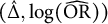 decomposition for each item pair (Figure 5) reveals structural features that depart from a simple Rasch model.
$\iota ^*$
 -decomposition plot for 56 inductive reasoning tasks (Golino & Gomes, Reference Golino, Gomes, Golino, Gomes, Amantes and Coelho2015). Each marker is one item pair, plotted at
$(\hat {\Delta }_{ij}, \log (\widehat {\mathrm {OR}}_{ij}))$
-decomposition plot for 56 inductive reasoning tasks (Golino & Gomes, Reference Golino, Gomes, Golino, Gomes, Amantes and Coelho2015). Each marker is one item pair, plotted at
$(\hat {\Delta }_{ij}, \log (\widehat {\mathrm {OR}}_{ij}))$
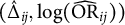 , with two cluster glyphs flanking the coordinate (left = item i, right = item j), joined by an arrow when the implication is unidirectional and by a plain segment when bidirectional. Within-cluster pairs (identical flanking glyphs) concentrate near the y-axis; between-cluster directed pairs (different flanking glyphs) fan out to the right. Gray lines: first principal components of between-cluster alignments. Shaded bands: (median) non-significance regions (
$\alpha =0.05$
, with two cluster glyphs flanking the coordinate (left = item i, right = item j), joined by an arrow when the implication is unidirectional and by a plain segment when bidirectional. Within-cluster pairs (identical flanking glyphs) concentrate near the y-axis; between-cluster directed pairs (different flanking glyphs) fan out to the right. Gray lines: first principal components of between-cluster alignments. Shaded bands: (median) non-significance regions (
$\alpha =0.05$
 ).
).

Figure 5 Long description
The X-axis represents Delta - Directional asymmetry, ranging from -2 to 8, with labels easy to hard on the left and hard to easy on the right. The Y-axis represents log O R - Symmetric association, ranging from -2 to 8.
Data points are pairs of items represented by two cluster glyphs. Within-cluster pairs, where both glyphs are identical, are concentrated near the Y-axis at Delta equals 0. Between-cluster pairs, featuring different glyphs joined by arrows or segments, fan out toward the positive X-axis.
A legend in the top right identifies seven cognitive levels by color and shape:
* Red circle: Pre-Operational
* Blue triangle: Primary
* Green square: Concrete
* Purple diamond: Abstract
* Orange asterisk: Formal
* Brown plus: Systematic
* Pink cross: Meta-systematic
Gray diagonal lines indicate the first principal components of between-cluster alignments. Shaded gray bands represent non-significance regions for association (horizontal band around Y equals 0) and directionality (vertical band around X equals 0).
Within-cluster pairs: Within-cluster item pairs concentrate near the y-axis, showing little directionality—consistent with items sharing similar difficulties within each stage. However,
$\log (\widehat {\mathrm {OR}})$
 values vary markedly across clusters, from roughly 5–7 for Pre-Operational pairs down to 1–2.5 for Systematic and Meta-systematic pairs. Since within-scale expected
$\log (\mathrm {OR})$
values vary markedly across clusters, from roughly 5–7 for Pre-Operational pairs down to 1–2.5 for Systematic and Meta-systematic pairs. Since within-scale expected
$\log (\mathrm {OR})$
 is a monotone increasing function of the latent variance (Equation (12)), this vertical stratification suggests that each stage operates with a different effective latent variance.
Between-cluster directed pairs: Between-cluster directed links fan out toward increasing
$\hat {\Delta }$
 and decreasing
$\log (\widehat {\mathrm {OR}})$
and decreasing
$\log (\widehat {\mathrm {OR}})$
 . Virtually all lie in the
$\hat {\Delta }>0$
. Virtually all lie in the
$\hat {\Delta }>0$
 region, confirming a cumulative “hard
$\to $
region, confirming a cumulative “hard
$\to $
 easy” structure. However, unlike the Rasch case, where between-pair
$\log (\mathrm {OR})$
easy” structure. However, unlike the Rasch case, where between-pair
$\log (\mathrm {OR})$
 would be approximately constant (horizontal alignments), these pairs follow diagonal patterns (gray lines on the figure). Within each pair type, the positive slopes indicate that items within a stage are not equally discriminating. Since
$\log (\mathrm {OR})$
would be approximately constant (horizontal alignments), these pairs follow diagonal patterns (gray lines on the figure). Within each pair type, the positive slopes indicate that items within a stage are not equally discriminating. Since
$\log (\mathrm {OR})$
 depends on the product
$a_i\,a_j$
depends on the product
$a_i\,a_j$
 of item discriminations (Equation (B.1)), this is a departure from the Rasch assumption that may reflect differences in item complexity (Bolt, Reference Bolt2022; Samejima, Reference Samejima2000), and the tightness of each alignment suggests that discrimination covaries smoothly with difficulty rather than varying randomly. Across pair types, adjacent stages show higher
$\log (\widehat {\mathrm {OR}})$
of item discriminations (Equation (B.1)), this is a departure from the Rasch assumption that may reflect differences in item complexity (Bolt, Reference Bolt2022; Samejima, Reference Samejima2000), and the tightness of each alignment suggests that discrimination covaries smoothly with difficulty rather than varying randomly. Across pair types, adjacent stages show higher
$\log (\widehat {\mathrm {OR}})$
 than distant ones, reflecting a graded latent correlation structure consistent with Equation (13), but this correlation between adjacent stages tends to decrease in higher stages, for comparable difficulty gaps. This might suggest some kind of progressive differentiation in cognitive abilities.
Together, these patterns support a mixed continuity/discontinuity picture: the within-cluster
$\log (\widehat {\mathrm {OR}})$
 stratification indicates stage-like groupings with distinct measurement properties, while the graded between-cluster diagonals indicate a hierarchically correlated developmental continuum. The data are not well described by either a single Rasch scale (which would produce a single horizontal band) or by fully independent stages (which would produce near-zero between-cluster
$\log (\widehat {\mathrm {OR}})$
stratification indicates stage-like groupings with distinct measurement properties, while the graded between-cluster diagonals indicate a hierarchically correlated developmental continuum. The data are not well described by either a single Rasch scale (which would produce a single horizontal band) or by fully independent stages (which would produce near-zero between-cluster
$\log (\widehat {\mathrm {OR}})$
 ).
).
Read as a diagnostic for downstream modeling, the joint pattern points to a specific class of model. Vertical stratification across stages indicates discrimination heterogeneity between clusters, while the positive slopes of the within-pair-type alignments indicate that, within a stage, discrimination is itself an increasing function of difficulty—the structural signature of items requiring multiple ordered cognitive operations. This is the regime in which a free-discrimination 2PL is unparsimonious: fitting one would recover
$a_i$
 values that correlate with
$\delta _i$
values that correlate with
$\delta _i$
 as an artifact of the symmetric link rather than as a substantive parameter (Bolt, Reference Bolt2022; Samejima, Reference Samejima2000). The appropriate next-step model is therefore not a 2PL with free discriminations, but an item-complexity/asymmetric-IRF model in which the discrimination–difficulty link is built into the response function, a path still to be explored on these data.
4.2.2 The dimensional implication graph
The final DIG is plotted in Figure 6. The seven SBM-recovered clusters, as noted above, coincide exactly with the seven expected Piagetian developmental stages and are materialized as ellipses on the figure. Significant links (
$p<0.05$
 , after BY adjustment) are shown as gray arrows: within-cluster symmetric links as double-headed arrows, and between-cluster directed links as single-headed arrows. Because of the high number of between-cluster links, and thanks to the clean within/between separation, all oriented links from one cluster to another are summarized as a single large arrow, with a label indicating the number of significant links included. Five log-OR levels, detected by k-means clustering on the MDS-derived associative coordinates, are marked as horizontal dashed lines, and item success rates are shown in parentheses within nodes.
Dimensional implication graph for 56 inductive reasoning tasks (Golino & Gomes, Reference Golino, Gomes, Golino, Gomes, Amantes and Coelho2015). Double-headed arrows: within-cluster symmetric links. Wider single-headed arrows: between-cluster directed links (labels give the count). Horizontal dashed lines: five log-OR levels. Diagonal dotted line: direction of increasing success rates (shown in parentheses).

Figure 6 Long description
The graph is organized on a coordinate system with a diagonal dotted line labeled Difficulty gradient running from the top-left to the bottom-right. Six shaded elliptical clusters are positioned along this gradient.
* The Primary cluster is at the top-left, containing items i 1 through i 16 with high success rates between 0.92 and 0.98. It is sub-labeled Pre-Operational.
* The Concrete cluster follows, containing items i 17 through i 24 with success rates between 0.71 and 0.81.
* The Abstract cluster is located near the center, containing items i 25 through i 32 with success rates between 0.44 and 0.52.
* The Formal cluster is positioned below the horizontal axis, containing items i 33 through i 41 with success rates between 0.20 and 0.29.
* The Systematic cluster is further down the gradient, containing items i 42 through i 48 with success rates between 0.09 and 0.12.
* The Meta-systematic cluster is at the bottom-right, containing items i 49 through i 56 with the lowest success rates between 0.02 and 0.04.
Within clusters, nodes are connected by thin double-headed arrows. Between clusters, thick grey single-headed arrows point from easier clusters toward more difficult ones, labeled with counts such as 64, 63, 62, 34, and 13. Five horizontal dashed lines mark log-O R levels at 2.61, 2, 1.5, 1, and negative 0.5.
Table 3 provides a quantitative summary of detected links. Two striking patterns emerge.
Summary of detected links across the seven clusters recovered by the SBM, ordered by decreasing success rate

Table 3 Long description
The table consists of 8 columns and 8 rows. The column headers are: P O, P r, C o, A b, F o, S y, and M S. The row headers represent seven clusters: 1-Pre-operational, 2-Primary, 3-Concrete, 4-Abstract, 5-Formal, 6-Systematic, and 7-Meta-systematic.
Diagonal entries (bold) represent within-cluster symmetric links:
- 1-Pre-operational (P O): 28
- 2-Primary (P r): 26
- 3-Concrete (C o): 13
- 4-Abstract (A b): 21
- 5-Formal (F o): 17
- 6-Systematic (S y): 20
- 7-Meta-systematic (M S): 27
Lower triangle entries represent between-cluster directed links:
- Row 2 (Primary): 63 in P O
- Row 3 (Concrete): 64 in P O, 64 in P r
- Row 4 (Abstract): 62 in P O, 64 in P r, 64 in C o
- Row 5 (Formal): 1 in P O, 61 in P r, 64 in C o, 64 in A b
- Row 6 (Systematic): 13 in C o, 34 in A b, 63 in F o
- Row 7 (Meta-systematic): 1 in F o, 34 in S y
Upper triangle entry:
- Row 1 (Pre-operational) at column P r: 1 (representing a single between-cluster symmetric link).
Empty cells indicate zero links.
Note: Diagonal entries (bold): within-cluster symmetric (associative) links, out of a maximum of
$\binom {8}{2}=28$
 . Lower triangle: between-cluster directed (implicative) links, out of a maximum of
$8\times 8=64$
. Lower triangle: between-cluster directed (implicative) links, out of a maximum of
$8\times 8=64$
 . The single between-cluster symmetric link (items 4–16) is shown in the upper triangle at position (PO, Pr). Empty cells indicate zero links.
Within-cluster symmetric links: All within-cluster links are of the symmetric (bidirectional) type, confirming the stage-like homogeneity expected when items within a cluster share similar difficulties. The density is highest for Pre-Operational (28/28) and Meta-systematic (27/28), and lowest for Concrete (13/28) and Formal (17/28), suggesting that the middle stages exhibit more internal heterogeneity.
Between-cluster directed links: All between-cluster links are directed, consistently oriented from harder to easier stages—no link goes in the reverse direction. However, the pattern is not purely cumulative: the table reveals a characteristic diagonal form in which backward implication links decrease with developmental distance. For instance, Formal items imply virtually all Abstract (64/64) and Concrete (64/64) items, most Primary items (61/64), but almost no Pre-Operational items (1/64). This fading of implication with developmental distance is the signature of an unfolding rather than a purely cumulative structure (Davison, Reference Davison1977; Davison et al., Reference Davison, Robbins and Swanson1978; Kohlberg, Reference Kohlberg and Goslin1969): each stage primarily implies adjacent stages within a limited developmental window, beyond which the statistical link fades as earlier skills are superseded rather than merely accumulated—a developmental-distance counterpart to the within-pair correlation weakening noted earlier in the decomposition plot. The contrast with the canonical 7-node cumulative case schematized in Figure 2 is informative: there, every harder node implies every easier node and the table of links would be uniformly filled below the diagonal; here, the lower triangle visibly thins out away from the diagonal. While part of this fade may be attributable to the reduced statistical power of the asymmetry test for pairs with very different success rates—where the discordant cell
$\pi _{a\bar {b}}$
 becomes sparse and inflates the variance of
$\hat {\Delta }$
becomes sparse and inflates the variance of
$\hat {\Delta }$
 —the same cell-sparsity/power-loss mechanism applies to genuine cumulative Rasch scales, where the canonical pattern (every harder item implying every easier item, including across wide difficulty gaps) is nevertheless empirically observed; the graded fade documented here is, therefore, not naturally attributable to power loss alone. Possible substantive explanations for this fading association phenomenon would point instead to processes, such as replacement or differentiation.
Difficulty gradient: Both figures display a clear difficulty gradient from easy items with high association (upper left) to hard items with low association (lower right). On Figure 6, this gradient is materialized as a dotted diagonal line labeled “Difficulty gradient,” running from the Pre-Operational cluster in the upper left to the Meta-systematic cluster in the lower right. Rotating the axes would recover the unidimensional difficulty continuum of a 2PL model, but the
$\iota ^*$
 -decomposition deliberately keeps the two components separate, making visible structural features—vertical stratification, discrimination heterogeneity, and the within/between separation—that a single IRT difficulty parameter would collapse.
Overall, the DIG simultaneously captures stage-like clustering (dense symmetric association within stages) and developmental ordering (directed implications cascading across stages within a limited window), revealing a structure intermediate between strict cumulativity and strict stage independence. The decomposition plot further disentangles two distinct sources of heterogeneity: differences in effective latent variance across stages (vertical stratification of within-cluster pairs) and item-level discrimination differences within stages (positive slopes of between-cluster alignments). The only cross-cluster symmetric link—between items 4 and 16 (Pre-Operational and Primary)—is consistent with a floor effect at the easy end of the continuum; no symmetric links cross boundaries between middle or advanced stages.
5 Discussion
This article introduced the
$\iota $
 -index, a measure of asymmetric statistical dependence designed to detect directional structures in multivariate binary data. The index synthesizes information from both positive and contrapositive evidence to quantify directional strength, and it yields a Rasch-metric interpretation under monotone item response models. Importantly, while the
$\iota $
-index, a measure of asymmetric statistical dependence designed to detect directional structures in multivariate binary data. The index synthesizes information from both positive and contrapositive evidence to quantify directional strength, and it yields a Rasch-metric interpretation under monotone item response models. Importantly, while the
$\iota $
 -index may uncover structures resembling developmental progressions or prerequisite relations, it does not identify causal effects in the counterfactual sense. Its purpose is exploratory: to reveal organized, directional patterns of association, in the form of what we call DIGs, that may support substantive theory building, item selection, or dimensional reduction.
The distinction between directed dependence and causality is essential. Causal inference from observational data requires strong assumptions—such as no unmeasured confounding, positivity, and well-defined counterfactuals (Imbens & Rubin, Reference Imbens and Rubin2015; Pearl, Reference Pearl2009)—that are not imposed in the present framework. Accordingly, the
$\iota $
 -index should be viewed as a tool for identifying structural asymmetries in the joint distribution of responses. Such asymmetries may arise from cognitive prerequisites, developmental ordering, or latent variable hierarchies, but causal conclusions would require additional design- or model-based assumptions beyond the scope of this work.
Building on previous proposals (Gras, Reference Gras1996; Loevinger, Reference Loevinger1947) that assess the rarity of counter-examples for a rule
$A\rightarrow B$
 , the
$\iota $
, the
$\iota $
 -index additionally incorporates its contrapositive
$\bar {B}\rightarrow \bar {A}$
-index additionally incorporates its contrapositive
$\bar {B}\rightarrow \bar {A}$
 . Both components are integrated into a product of imbalance ratios, connecting the index to the OR—which emerges as the geometric mean of
$\iota $
. Both components are integrated into a product of imbalance ratios, connecting the index to the OR—which emerges as the geometric mean of
$\iota $
 in both directions. The pair
$(\iota _{A\rightarrow B},\iota _{B\rightarrow A})$
in both directions. The pair
$(\iota _{A\rightarrow B},\iota _{B\rightarrow A})$
 thus contains strictly more information than OR alone, providing association and direction within a unified structure. A further property is that the index evaluates directed dependence on a Rasch metric, leading to graphical representations where items belonging to a common Rasch scale are aligned, with all links oriented in the difficult
$\rightarrow $
thus contains strictly more information than OR alone, providing association and direction within a unified structure. A further property is that the index evaluates directed dependence on a Rasch metric, leading to graphical representations where items belonging to a common Rasch scale are aligned, with all links oriented in the difficult
$\rightarrow $
 easy direction. In more general settings, the graph may take arbitrary forms, bridging the gap between purely graphical and purely dimensional representations.
When a dimensional structure underlies the data, a pure network approach, such as exploratory graph analysis (Golino & Epskamp, Reference Golino and Epskamp2017; Golino & Gomes, Reference Golino, Gomes, Golino, Gomes, Amantes and Coelho2015), will detect item clusters as factors but miss how these clusters form a hidden cumulative scale—as observed in the developmental data above. DIGs may thus be viewed as a directional, Rasch-aware extension of EGA, able to uncover embedded dimensional structures together with their implicative ordering.
However, DIGs are not designed as a strategy for Rasch parameter estimation, for which dedicated software will provide better estimates. More work is needed to study the robustness of
$\iota ^{\ast}$
 estimates under various conditions of sample size, effect size, and dependence structure.
In the Rasch case, a null
$\iota ^{\ast}$
 corresponds to a null difficulty difference, so not all links within a true Rasch scale would be retained—only those between sufficiently distant items. The visual alignment remains a useful diagnostic, and retaining only items with significant implication links provides a natural pruning strategy when a simplified scale is desired.
Beyond the Rasch model, this approach has the ability to detect more generic cumulative structure, appearing in the graph as chains of implication links, all going from the rarest to the most common items, but not necessarily aligned in the graphical representation. This may be viewed as a non-parametric item scaling procedure, along the lines of Mokken scaling (Mokken, Reference Mokken1971), but with the additional advantages that multiple scales, or only partially cumulative scales, can be visually detected.
The pairwise nature of the computation also offers practical advantages: missing data are handled naturally by computing frequencies on available pairs, the computation is easily parallelizable, and DIG construction may help reveal local dependencies in a generalized cumulative structure, along the lines of the mixed network-IRT model of Ueno (Reference Ueno2002).
We believe that this approach could be useful in a number of applied psychometric contexts, including mixed dimensional/categorical representation of mental disorders (Borsboom, Reference Borsboom2017; Borsboom et al., Reference Borsboom, Cramer, Schmittmann, Epskamp and Waldorp2011), identification of the number of factors in cognitive tasks (Golino & Epskamp, Reference Golino and Epskamp2017), or item selection in scale construction—where a DIG may provide a fast visual indication of which items deviate from an expected alignment.
More broadly, the exploratory detection of directed dependencies within large sets of binary indicators is of growing interest. The DIG approach could complement structure-learning methods by narrowing the search space when latent variables are suspected (Colombo et al., Reference Colombo, Maathuis, Kalisch and Richardson2012; Ogarrio et al., Reference Ogarrio, Spirtes and Ramsey2016), or serve as a lag-screening tool in multivariate binary time series (Runge, Reference Runge, Peters and Sontag2020).
Data availability statement
Code to reproduce the empirical illustration is publicly available at https://github.com/yvonnicknoel/iota-implication-graphs. The Inductive Reasoning Developmental Test dataset analyzed in the empirical illustration was made publicly available by Golino and Epskamp (Reference Golino and Epskamp2017).
Acknowledgements
The author wishes to thank Hudson Golino and Sacha Epskamp for making the Inductive Reasoning dataset available. The author is also indebted to an anonymous reviewer whose suggestion led to a sharper formulation of the marginal asymmetry identity and the dimensional analysis built upon it.
Author contributions
Y.N. is the sole author and is responsible for all aspects of the work, including conceptualization, methodology, formal analysis, software, writing of the original draft, and review and editing.
Funding statement
This research received no specific grant from any funding agency, commercial, or not-for-profit sectors.
Competing interests
The author declares none.
Ethical standards
The research meets all ethical guidelines, including adherence to the legal requirements of the study country. The empirical illustration relies solely on a publicly available, de-identified secondary dataset and involved no new data collection from human participants.
Use of AI tools
No artificial intelligence tools were used in the conception, analysis, or writing of this manuscript.
A Adjustment for observed covariates
The inferential framework described in the article can be extended in a straightforward manner to account for observed covariates. Let
$C\in \{0,1\}$
 denote a binary covariate and consider the conditional joint distributions of A and B within strata
$C=c$
denote a binary covariate and consider the conditional joint distributions of A and B within strata
$C=c$
 .
.
For each stratum c, we define the conditional implication index

which admits the same decomposition as in the marginal case:

or, on the log scale,

Inference is conducted on both components within each stratum using the same two-step strategy as in the marginal case: a one-sided Wald test for positive association, followed by a two-sided Wald test for asymmetry.
Heterogeneity can be assessed using Cochran’s Q statistic (Cochran, Reference Cochran1954) (ideally when more than two strata are available) or by inspection when stratum-specific estimates diverge markedly. If stratum-specific estimates are heterogeneous—for instance, showing opposite signs for
$\log (\mathrm {OR})$
 or
$\Delta $
or
$\Delta $
 across levels of C—this pattern suggests confounding or effect modification, and the marginal association may be entirely spurious, as in Simpson’s paradox. Significant heterogeneity warrants reporting stratum-specific effects rather than common estimates. Confounding may of course affect both components differently across strata.
Conversely, if stratum-specific estimates are homogeneous—pointing in the same direction with comparable magnitudes—common estimates are legitimate. In these cases, pooling stratum-specific estimates is preferable to simply analyzing the marginal table, which may conflate within-stratum associations with between-stratum variation in base rates, potentially yielding spurious associations. Pooling avoids this by averaging within-stratum effects, thereby removing confounding by C.
When homogeneity holds, stratum-specific estimates may be pooled on the log scale using inverse-variance weighting (Agresti, Reference Agresti2013; Cochran, Reference Cochran1954). Let
$\log (\widehat {\mathrm {OR}})_c$
 and
$\widehat {\Delta }_c=\log (\pi _{\bar a b\mid c}/\pi _{a\bar b\mid c})$
and
$\widehat {\Delta }_c=\log (\pi _{\bar a b\mid c}/\pi _{a\bar b\mid c})$
 denote the stratum-specific estimators, with estimated variances
$\widehat {V}^{\mathrm {OR}}_c$
denote the stratum-specific estimators, with estimated variances
$\widehat {V}^{\mathrm {OR}}_c$
 and
$\widehat {V}^{\Delta }_c$
and
$\widehat {V}^{\Delta }_c$
 , respectively. The pooled estimators are

and

Wald tests for
$\log (\mathrm {OR})_{\mathrm {pool}}=0$
 and
$\Delta _{\mathrm {pool}}=0$
and
$\Delta _{\mathrm {pool}}=0$
 then provide tests of association and directional asymmetry adjusted for C. As in the marginal case, directional dependence is interpreted only when both components provide evidence against their respective null hypotheses.
B Marginal log odds ratio under the 2PL and Rasch models
This appendix derives the expected marginal log OR between pairs of items under the 2PL model, as a function of the latent trait variance and item discriminations, both within a single scale and across two correlated scales. The Rasch model is recovered as the special case of equal discriminations.
B.1 Within-scale log odds ratio
Consider two items
$X_i$
 and
$X_j$
and
$X_j$
 following a 2PL model with difficulties
$\delta _i$
following a 2PL model with difficulties
$\delta _i$
 and
$\delta _j$
and
$\delta _j$
 , discriminations
$a_i$
, discriminations
$a_i$
 and
$a_j$
and
$a_j$
 , and a normally distributed latent trait
$\theta \sim N(0, \sigma ^2)$
, and a normally distributed latent trait
$\theta \sim N(0, \sigma ^2)$
 . Conditional on
$\theta $
. Conditional on
$\theta $
 , responses are locally independent with
$P(X_k = 1 \mid \theta ) = 1/\{1 + \exp [-a_k(\theta - \delta _k)]\}$
, responses are locally independent with
$P(X_k = 1 \mid \theta ) = 1/\{1 + \exp [-a_k(\theta - \delta _k)]\}$
 . The Rasch model is the special case
$a_k = 1$
. The Rasch model is the special case
$a_k = 1$
 for all items.
This response function can be expressed as a threshold model (Birnbaum, Reference Birnbaum, Lord and Novick1968):
$X_k = 1$
 if and only if
$a_k\theta + e_k> a_k\delta _k$
if and only if
$a_k\theta + e_k> a_k\delta _k$
 , where
$e_k$
, where
$e_k$
 follows a standard logistic distribution with mean 0 and variance
$\pi ^2/3$
follows a standard logistic distribution with mean 0 and variance
$\pi ^2/3$
 (Camilli, Reference Camilli1994), independently of
$\theta $
(Camilli, Reference Camilli1994), independently of
$\theta $
 and of the other error terms. Defining the latent continuous variables
$Y_k = a_k\theta + e_k$
and of the other error terms. Defining the latent continuous variables
$Y_k = a_k\theta + e_k$
 , we have
$\mathrm {Var}(Y_k) = a_k^2\,\sigma ^2 + \pi ^2/3$
, we have
$\mathrm {Var}(Y_k) = a_k^2\,\sigma ^2 + \pi ^2/3$
 and
$\mathrm {Cov}(Y_i, Y_j) = a_i\,a_j\,\sigma ^2$
and
$\mathrm {Cov}(Y_i, Y_j) = a_i\,a_j\,\sigma ^2$
 , since the logistic errors
$e_i$
, since the logistic errors
$e_i$
 and
$e_j$
and
$e_j$
 are mutually independent and independent of
$\theta $
are mutually independent and independent of
$\theta $
 . The induced correlation between
$Y_i$
. The induced correlation between
$Y_i$
 and
$Y_j$
and
$Y_j$
 is therefore

Under the Rasch model (
$a_k=1$
 for all k), this simplifies to
$\sigma ^2/(\sigma ^2+\pi ^2/3)$
for all k), this simplifies to
$\sigma ^2/(\sigma ^2+\pi ^2/3)$
 , the latent-variable intraclass correlation coefficient used in logistic multilevel models (Snijders & Bosker, Reference Snijders and Bosker2012).
In general, this correlation depends on the discriminations
$a_i$
 and
$a_j$
and
$a_j$
 through their product, and therefore varies across item pairs. Under the Rasch model, however, this dependence vanishes: with
$a_k=1$
through their product, and therefore varies across item pairs. Under the Rasch model, however, this dependence vanishes: with
$a_k=1$
 for all items, the correlation is the same for all item pairs, since each
$Y_k$
for all items, the correlation is the same for all item pairs, since each
$Y_k$
 has the same variance and the covariance
$\sigma ^2$
has the same variance and the covariance
$\sigma ^2$
 does not depend on item difficulties. The marginal cell probabilities
$P(X_i = x_i,\, X_j = x_j)$
does not depend on item difficulties. The marginal cell probabilities
$P(X_i = x_i,\, X_j = x_j)$
 are determined by the bivariate distribution of
$(Y_i, Y_j)$
are determined by the bivariate distribution of
$(Y_i, Y_j)$
 together with the thresholds
$(\delta _i, \delta _j)$
together with the thresholds
$(\delta _i, \delta _j)$
 , so the marginal OR does, in principle, depend on item difficulties through those thresholds. However, for bivariate normal variables, the log OR is primarily governed by the latent correlation, with only a weak second-order dependence on the cut points. This is a classical result in the tetrachoric correlation literature (see, e.g., Becker & Clogg, Reference Becker and Clogg1988): the log OR between two dichotomized normal variables depends primarily on their latent correlation, with only a weak second-order sensitivity to the threshold locations. Since the tetrachoric correlation recovers the latent
$\rho (Y_i,Y_j)$
, so the marginal OR does, in principle, depend on item difficulties through those thresholds. However, for bivariate normal variables, the log OR is primarily governed by the latent correlation, with only a weak second-order dependence on the cut points. This is a classical result in the tetrachoric correlation literature (see, e.g., Becker & Clogg, Reference Becker and Clogg1988): the log OR between two dichotomized normal variables depends primarily on their latent correlation, with only a weak second-order sensitivity to the threshold locations. Since the tetrachoric correlation recovers the latent
$\rho (Y_i,Y_j)$
 under bivariate normality, and this correlation is the same for all item pairs within a Rasch scale, the log OR is approximately constant across item difficulties.
More generally, the threshold impact remains modest when (i) items are not too extreme (moderate
$|\delta _k|/\sigma $
 ), (ii) difficulty grids are balanced so that midpoint effects tend to cancel, and (iii) the induced correlation is moderate. Under these conditions—typically met in well-constructed psychometric instruments—the variance-only approximation below provides an adequate summary, with deviations visible mainly for very easy or very difficult items (Figure 3).
Over the moderate range of
$\sigma $
 encountered in practice, the mapping
$\sigma \mapsto \mathbb {E}[\log (\mathrm {OR})_{\mathrm {within}}]$
encountered in practice, the mapping
$\sigma \mapsto \mathbb {E}[\log (\mathrm {OR})_{\mathrm {within}}]$
 is close to linear, so association strength grows approximately proportionally to
$\sigma $
is close to linear, so association strength grows approximately proportionally to
$\sigma $
 , which motivates a linear approximation. We use the logistic variance
$\pi ^2/3$
, which motivates a linear approximation. We use the logistic variance
$\pi ^2/3$
 as a scaling constant to relate the marginal log OR to the underlying correlation. This yields a convenient approximation:

Under the Rasch model, this reduces to
$(\pi ^2/3)\,\sigma ^2/(\sigma ^2 + \pi ^2/3)$
 , which is constant across item pairs and has a variance ratio form analogous to reliability coefficients in classical test theory (its accuracy for Rasch scales is illustrated in Figure 3). Under the 2PL model, the expected log OR depends on the product
$a_i\,a_j$
, which is constant across item pairs and has a variance ratio form analogous to reliability coefficients in classical test theory (its accuracy for Rasch scales is illustrated in Figure 3). Under the 2PL model, the expected log OR depends on the product
$a_i\,a_j$
 : pairs involving more discriminating items produce higher
$\log (\mathrm {OR})$
: pairs involving more discriminating items produce higher
$\log (\mathrm {OR})$
 .
.
B.2 Between-scale log odds ratio
Now consider two scales with latent traits
$\theta _1 \sim N(0,\ \sigma _1^2)$
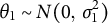 and
$\theta _2 \sim N(0,\ \sigma _2^2)$
and
$\theta _2 \sim N(0,\ \sigma _2^2)$
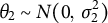 , with correlation
$\rho = \mathrm {Cor}(\theta _1,\ \theta _2)$
, with correlation
$\rho = \mathrm {Cor}(\theta _1,\ \theta _2)$
 . For item i on scale 1 (discrimination
$a_i$
. For item i on scale 1 (discrimination
$a_i$
 ) and item j on scale 2 (discrimination
$a_j$
) and item j on scale 2 (discrimination
$a_j$
 ), the underlying continuous variables are
$Y_i = a_i\theta _1 + e_i$
), the underlying continuous variables are
$Y_i = a_i\theta _1 + e_i$
 and
$Y_j = a_j\theta _2 + e_j$
and
$Y_j = a_j\theta _2 + e_j$
 , with
$\mathrm {Var}(Y_i) = a_i^2\,\sigma _1^2 + \pi ^2/3$
, with
$\mathrm {Var}(Y_i) = a_i^2\,\sigma _1^2 + \pi ^2/3$
 ,
$\mathrm {Var}(Y_j) = a_j^2\,\sigma _2^2 + \pi ^2/3$
,
$\mathrm {Var}(Y_j) = a_j^2\,\sigma _2^2 + \pi ^2/3$
 , and
$\mathrm {Cov}(Y_i,\ Y_j) = a_i\,a_j\,\rho \,\sigma _1\sigma _2$
, and
$\mathrm {Cov}(Y_i,\ Y_j) = a_i\,a_j\,\rho \,\sigma _1\sigma _2$
 . The induced correlation is

and the between-scale log OR follows by the same
$(\pi ^2/3)$
 scaling:

When
$\sigma _1 = \sigma _2 = \sigma $
 and
$\rho = 1$
and
$\rho = 1$
 (i.e., items on the same scale), this reduces to Equation (B.1). When
$\rho = 0$
(i.e., items on the same scale), this reduces to Equation (B.1). When
$\rho = 0$
 (independent scales), the between-scale log OR vanishes, confirming that marginally independent latent traits induce no marginal association between their respective items. For intermediate correlations, the between-scale log OR takes values between zero and the within-scale levels, governed by the latent covariance
$\rho \,\sigma _1\sigma _2$
(independent scales), the between-scale log OR vanishes, confirming that marginally independent latent traits induce no marginal association between their respective items. For intermediate correlations, the between-scale log OR takes values between zero and the within-scale levels, governed by the latent covariance
$\rho \,\sigma _1\sigma _2$
 scaled by the geometric mean of the total variances.
Obviously, approximations B.1 and B.2 neglect the impact of item difficulties. However, for moderate correlations and not-too-extreme marginals, they were found in simulations to provide satisfactory approximations; we include them as an argument for separability and as a basis for easy-to-interpret graph layouts.
An important consequence for the
$(\hat {\Delta },\log (\widehat {\mathrm {OR}}))$
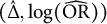 decomposition plot concerns the slope of within-pair-type alignments. Under the Rasch model,
$\log (\mathrm {OR})$
decomposition plot concerns the slope of within-pair-type alignments. Under the Rasch model,
$\log (\mathrm {OR})$
 is approximately constant within each pair type (since the induced correlation does not depend on individual items):
$\hat {\Delta }$
is approximately constant within each pair type (since the induced correlation does not depend on individual items):
$\hat {\Delta }$
 varies with the difficulty gap but
$\log (\mathrm {OR})$
varies with the difficulty gap but
$\log (\mathrm {OR})$
 does not, producing horizontal alignments. Under the 2PL model,
$\log (\mathrm {OR})$
does not, producing horizontal alignments. Under the 2PL model,
$\log (\mathrm {OR})$
 depends on
$a_i\,a_j$
depends on
$a_i\,a_j$
 , so items with higher discriminations produce both stronger association and—through steeper response functions—more extreme difficulty contrasts. The approximate independence between
$\hat {\Delta }$
, so items with higher discriminations produce both stronger association and—through steeper response functions—more extreme difficulty contrasts. The approximate independence between
$\hat {\Delta }$
 and
$\log (\mathrm {OR})$
and
$\log (\mathrm {OR})$
 breaks down, and within-pair-type alignments acquire a positive slope. Non-zero slopes in the decomposition plot thus serve as a visual diagnostic for discrimination heterogeneity.


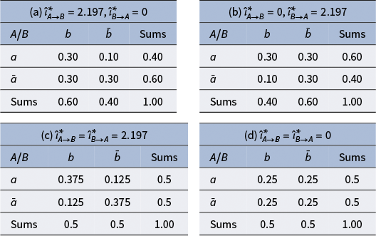



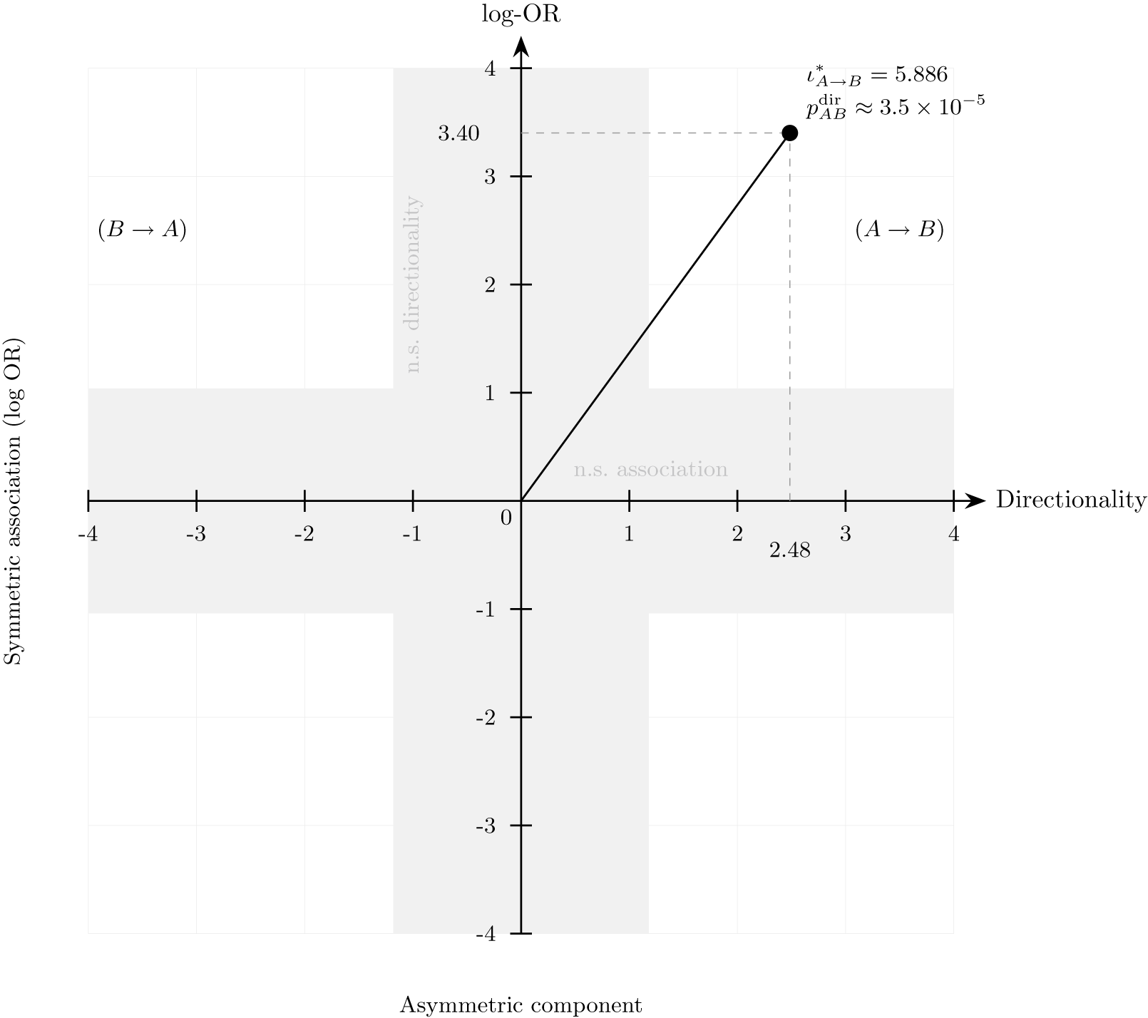


 ), computed from the asymptotic standard errors of



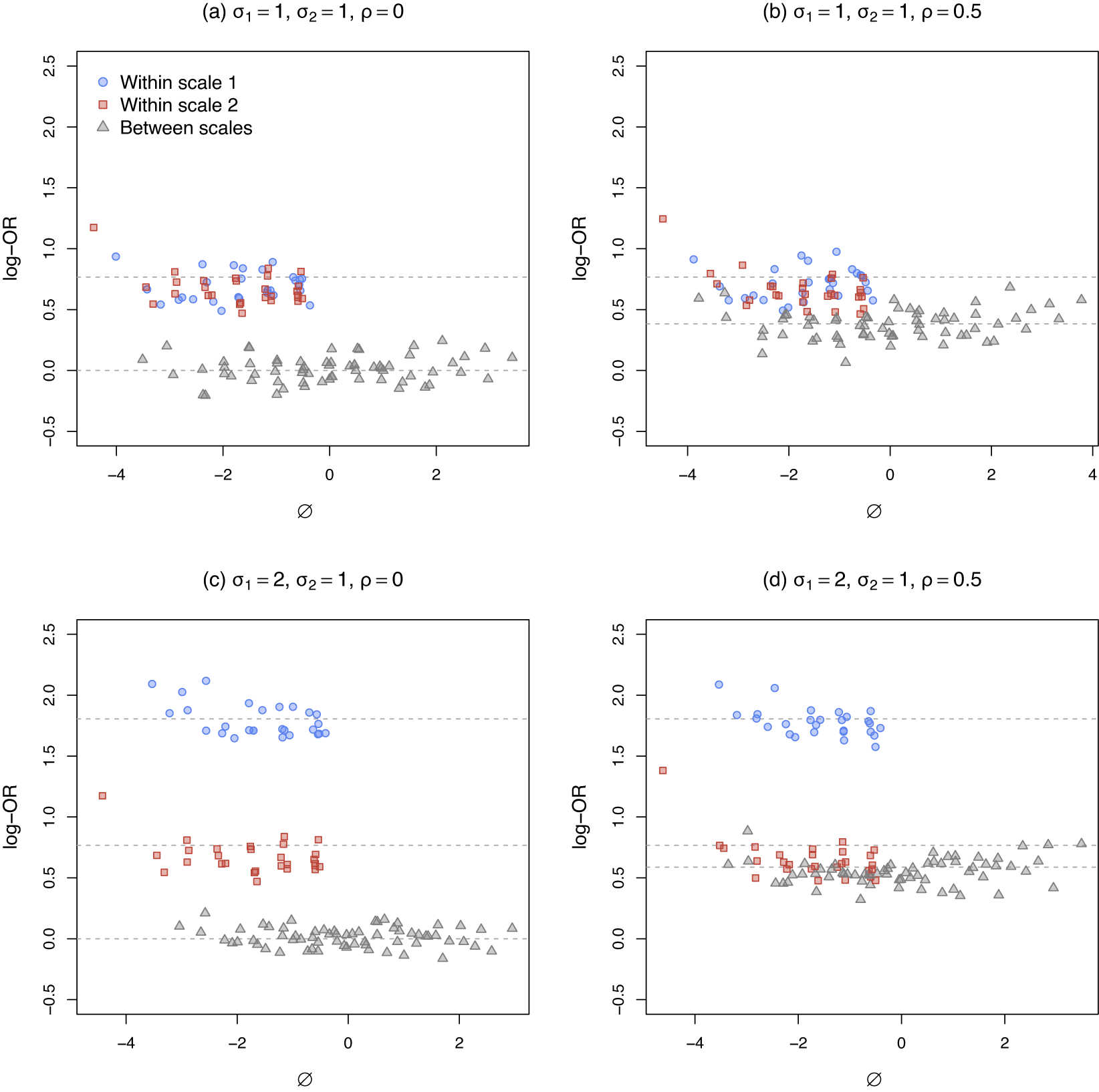


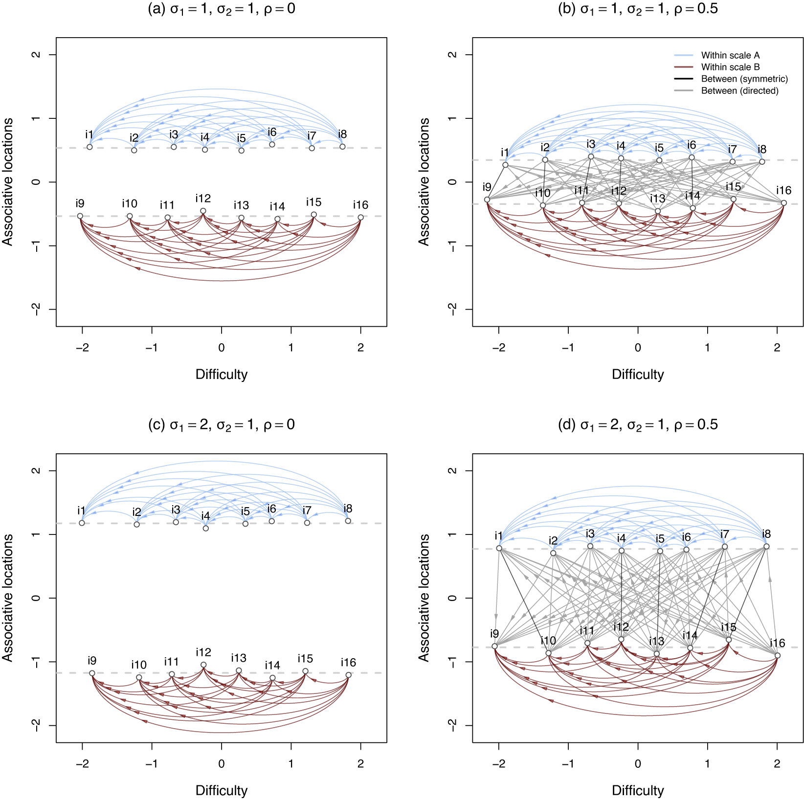


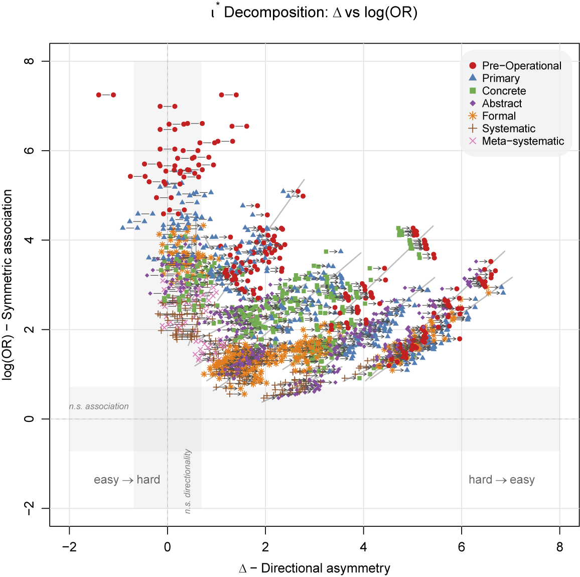


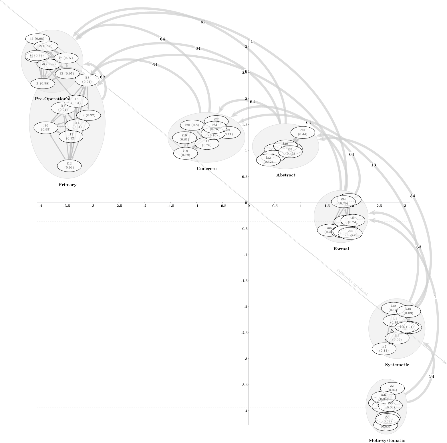
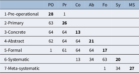

 Open access

