


1 Introduction
We develop a model of stability and constraint between multiple attitudes, measured on ordinal scales. We are motivated by the fact that attitude stability and constraint with related attitudes are two of the three factors, together with influence on other newly formed attitudes, which are used to assess an attitude’s degree of crystallization (Sears and Funk Reference Sears and Funk1999).Footnote 1 Understanding whether political attitudes are stable is essential for the study of public opinion, participatory behavior, and how people relate to politics more broadly.
Stability is an attitude’s resistance to the effects of change-inducing shocks (Erber, Hodges, and Wilson Reference Erber, Hodges and Wilson1995). We conceptualize attitude stability as arising from the interplay of the resistance to change and the pressures to change (Sears Reference Sears1983). An attitude’s stability is indicative of its strength (Prislin Reference Prislin1996) and of how well it predicts other attitudes and behaviors (Glasman and Albarracín Reference Glasman and Albarracín2006). Constraint between attitudes refers to the extent to which a change in one necessitates compensating changes in closely related but distinct attitudes (Converse Reference Converse and Apter1964). It is one metric for the attitude’s influence. The degree of constraint among a group of attitudes speaks to whether they form a constrained attitude system. We define an attitude system as an arrangement of related attitudes that are functionally interdependent.Footnote 2 The stability of individual attitudes and the constraint between theoretically related attitudes together capture the degree to which people hold meaningful political attitudes (Converse Reference Converse and Apter1964).
We employ dynamic discrete choice methods to model the joint evolution of attitudes as reflecting: observed covariates and controls, e.g., demographics, permanent, multidimensional unobserved heterogeneity, wave- or time-specific effects, and shocks disciplined by a flexible covariance structure, allowing for both persistence of shocks over time as well as spillovers between attitudes.
“Shocks” or “errors” capture variance of all unobserved model components. In keeping with the idea of a dynamic attitude system, the process of attitudinal change proceeds as follows: 1) an equilibrium is maintained in the system; 2) a shock causes a change in one attitude; and 3) this change then triggers a chain of shock spillovers to functionally interdependent attitudes in the system.
We assume that every period, every attitude is perturbed by a shock of its own, which we call “own shocks.” For identification, we assume that shocks are not contemporaneously correlated across attitudes but allow shocks to impact the shocks to other attitudes in subsequent time periods without further restrictions. We call these correlations of shocks over time “spillover effects” or “shock spillovers.” Since the triggering shock occurs one period before subsequent spillovers, this restriction identifies the causal direction of attitude change within the system.
Critically, our model handles the ordered, discrete nature of attitudes’ measurement scales. To the best of our knowledge, there is no off-the-shelf statistical software or package that allows the joint determination of ordinal variables with shocks correlated over outcomes and over time.Footnote 3 Compared to prior approaches, our model captures more fully the data-generating process by incorporating a wide array of sources of attitudinal variance and by accounting for the joint determination of attitudes that theory describes as related.
We present two analytic approaches. First, variance decomposition characterizes the stability of an attitude via the proportion of variance explained by each model component. The greater the proportion attributable to time-invariant, person-specific effects and infrequently-changing explanatory variables, the higher is its inherent stability.
Our second analytical approach consists of estimating the size, direction, and persistence of shock spillovers between theoretically related attitudes. It quantifies each attitude’s susceptibility or resistance to spillovers from other attitudes, providing insights into the degree to which the studied attitudes reflect an overarching attitude system and their relative degree of influence (Freeder, Lenz, and Turney Reference Freeder, Lenz and Turney2019). Examining the constraint between attitudes informs theories about why people hold the bundles of attitudes that they do. For example, this provides an avenue for testing the theory of Lenz (Reference Lenz2012), arguing that support for a candidate structures policy attitudes.Footnote 4
We describe two applications using the British Election Study Internet Panel (BESIP) and the U.S. General Social Survey (GSS). From BESIP, we examine five attitudes used to predict political behavior: the sense of civic duty to vote, people’s trust in Members of Parliament, internal political efficacy, external political efficacy, and satisfaction with how democracy is working in the UK. We focus on these because of their importance in the literature, because they are theoretically and empirically related, and because they are likely influenced by the same pressures to change (e.g., corruption scandals and referendums). We expect these attitudes to be part of a dynamic attitude system, based on their well-documented association and their moderating effect on each other.
We preview several results: first, we find that all attitudes are stable; second, we identify two attitude systems, one capturing how people see their role in politics, and another on how they evaluate the external political world; and third, we document a limited role for time-invariant unobserved heterogeneity in explaining civic duty to vote and trust in MPs. Internal efficacy has far more influence on civic duty than vice versa, suggesting that it is relatively important in how people see their role in politics. The second attitude system, how people evaluate the external political world, is less constrained, with the three attitudes exerting minimal to moderate influence on each other.
The GSS application examines ideological identification, party identification, and attitudes toward immigrants, military spending, welfare spending, and environmental spending. We expect these attitudes to be related, given work showing the growing influence of party identification on ideological identification, and the many studies on the influence of symbolic identities on issue attitudes. Both ideological and party identification are fairly stable, with a substantial share of their variance explained by time-invariant individual traits. Transitory shocks suggest measurement error and/or expressive responding. The four issue positions are unstable. Transitory own shocks account for most of the variance in issue attitudes, hinting at attitudinal instability caused by frequently-changing consideration pools (Zaller and Feldman Reference Zaller and Feldman1992), random measurement error, and differential item functioning of survey instruments. This instability raises questions about the extent to which members of the public hold true attitudes about these issues. Even if shocks reflect only changing consideration pools, the only source indicative of true attitude change, concerns would remain about how easily the public might be persuaded and the strength of their held attitudes.
2 Attitude Stability and Constraint
We overview key ideas in the study of attitudes, concerning stability and constraint within attitude systems. We expand on the comparison with existing methods in Appendix D of the Supplementary Material, including contrasting our results to reference models.
2.1 Attitude Stability
Work on the stability of political attitudes falls within seven broad categories. The first two operationalize stability as the extent to which respondents maintain their relative position in the distribution, employing test–retest correlations. A first set of papers computes rank correlations over time for attitudes measured across sets of two panel waves and interprets correlations as measures of stability (Freeder et al. Reference Freeder, Lenz and Turney2019). The second approach reports rank correlations for each individual’s attitude across time to evaluate whether correlations are stable. Focusing on rank correlations stresses the distinction between attitude changes that are broadly shared across the population and each individual’s relative position. By focusing exclusively on the latter, this approach does not capture shifts of the entire population (Green, Palmquist, and Schickler Reference Green, Palmquist and Schickler2002), nor does it decompose variance by sources. Such strategies do not provide point estimates for stability, making comparisons across attitudes challenging. Examples include Sears and Funk (Reference Sears and Funk1999) and Green et al. (Reference Green, Palmquist and Schickler2002).
A third approach involves absolute-agreement intraclass correlation coefficients (ICCs). These measure the degree of agreement between measurements made on the same individual in different waves. An attitude is perfectly stable if individuals report the same score across all waves. This approach considers both the correlation between variables and systematic differences. However, it does not account for the ordered discrete nature of measures. Nor does it speak to different sources of attitudinal (in)stability. It requires balanced panels, precluding the use of all available data.Footnote 5
A fourth branch of the literature studies whether individuals return to their long-term attitude by developing a typology of trajectories for attitudes over time, e.g., some who never change their attitude, while others express persistent changes. The focus is on the share of people whose attitude never changes or returns promptly (Sears and Funk Reference Sears and Funk1999). There is no notion of how far different categories on the ordinal scale are from each other. This risks producing fragile estimates, since the likelihood of providing the exact same response might depend on the number of response categories. Fewer categories could increase the probability that respondents report the same attitude across waves and give the impression that attitudes measured with fewer options are more stable. In contrast, we employ a latent dependent variable with well-defined units relative to other variables in the model. For us, staying in the same cell is not critical or special, and has no effect on notions of stability. Instead, the relevant notion is how much the latent variable changes.Footnote 6
A fifth approach employs time-series methods, stressing measurement error, for stability at the population level. Examples include Krosnick (Reference Krosnick1991) and Feitosa and Galais (Reference Feitosa and Galais2020). Such a model cannot address spillovers, ordinal measures, individual-level characteristics, or time-specific factors.
The sixth approach uses linear panel models with autocorrelated shocks. These are the simplest models that include a rich set of controls and effects. A typical specification is
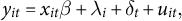 $ y_{it} = x_{it} \beta + \lambda _i + \delta _t + u_{it}, $
with
$ y_{it} = x_{it} \beta + \lambda _i + \delta _t + u_{it}, $
with
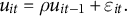 $ u_{it} = \rho u_{it-1} + \varepsilon _{it}. $
This model can only study each attitude in isolation, unable to speak to spillovers and attitude systems. Still, it does accommodate individual- and time-specific effects,
$ u_{it} = \rho u_{it-1} + \varepsilon _{it}. $
This model can only study each attitude in isolation, unable to speak to spillovers and attitude systems. Still, it does accommodate individual- and time-specific effects,
 $ \lambda _i $
and
$ \lambda _i $
and
 $ \delta _t $
, observable covariates
$ \delta _t $
, observable covariates
 $ x_{it} $
, and autoregressive shocks
$ x_{it} $
, and autoregressive shocks
 $ u_{it} $
. Stability is a statement about the persistence with which shocks today impact future values of the attitude, governed by the
$ u_{it} $
. Stability is a statement about the persistence with which shocks today impact future values of the attitude, governed by the
 $ \rho $
coefficient.
$ \rho $
coefficient.
Finally, another extension of linear panels is the linear dynamic panel model,
 $ y_{it} = x_{it} \beta + \lambda _i + \delta _t + \rho y_{it-1} + \varepsilon _{it} $
(Green and Palmquist Reference Green and Palmquist1994; Prior Reference Prior2010). This model’s distinguishing feature is the inclusion of a lag as a right-hand-side variable; its
$ y_{it} = x_{it} \beta + \lambda _i + \delta _t + \rho y_{it-1} + \varepsilon _{it} $
(Green and Palmquist Reference Green and Palmquist1994; Prior Reference Prior2010). This model’s distinguishing feature is the inclusion of a lag as a right-hand-side variable; its
 $ \rho $
coefficient reflects the impact of past variables on the attitude. Including lags raises endogeneity concerns, necessitating specific estimators (Arellano and Bond Reference Arellano and Bond1991). Stability is the degree to which past shocks, past individual- and time-specific effects, and past observables affect the attitude. This method shares all the aforementioned limitations of linear panel models.
$ \rho $
coefficient reflects the impact of past variables on the attitude. Including lags raises endogeneity concerns, necessitating specific estimators (Arellano and Bond Reference Arellano and Bond1991). Stability is the degree to which past shocks, past individual- and time-specific effects, and past observables affect the attitude. This method shares all the aforementioned limitations of linear panel models.
Against this background, we address the joint determination of attitudes, differentiating between own shocks and spillovers from related attitudes. This improves over the time series approach and linear panel models, which are silent on spillovers. The test–retest, ICC, and “typology” approaches do not quantify the effects of shocks, including measurement error. For us, own shocks capture (1) random measurement error, defined as the i.i.d. portion of the error term, (2) consideration pool randomness related to true latent attitudinal changeFootnote 7 (Zaller and Feldman Reference Zaller and Feldman1992), and (3) differential item functioning, differences in how individuals convert their latent attitude to survey question responses (Aldrich and McKelvey Reference Aldrich and McKelvey1977; Brady Reference Brady1985; Simas Reference Simas2018).Footnote 8 Also different, we model time-invariant differences between individuals flexibly, with a multidimensional random effect.Footnote 9 Moreover, we tackle the ordinalFootnote 10 nature of survey measures and treat explicitly the fact that the time between interviews varies across waves.
2.2 Constraint within Attitude Systems
The approaches above are silent on the constraint of multiple attitudes. Modeling attitudes jointly allows us to estimate the level of constraint between attitude pairs and the way shocks to one impact each of the others. Our approach identifies groups of attitudes that form attitude systems and the relative influence of attitudes within them. We operationalize an attitude’s influence as the proportion of “spillover variance”Footnote 11 in other attitudes explained by its spillovers.
Our framework improves over calculating correlations between attitudes at various points in time (Sears and Funk Reference Sears and Funk1999) because we model explicitly the processes through which shocks to one attitude influence others, accounting for multiple sources of variation. Traditionally, a pair of attitudes is considered as constraining each other if they maintain a relatively high correlation over time. Correlations recover the strength and direction of a linear association, regardless of the nature and source of changes. They do not adjust for confounders that might contribute to observed constraint, or lack thereof. Correlation-based approaches do not handle missing data well, often employing listwise or pairwise deletion as necessary. We consider multiple sources of attitudinal change across time and individuals, which can affect all attitudes in the system.
3 A Dynamic Discrete Choice Approach
We introduce a dynamic panel model for multiple attitudes. Attitudes are latent, observed imprecisely, via the Likert scales of survey questions. The textbook model closest to ours is ordered probit. We depart from it in three major ways: we study multiple dependent variables jointly; we employ a rich structure of heterogeneity and shocks, to capture interactions over time and across attitudes; and we accommodate unequal time between survey interviews.
We model attitudes as reflecting: 1) observed covariates and controls, e.g., demographics, 2) permanent, multidimensional, unobserved heterogeneity, 3) time-specific effects, and 4) shocks with a flexible covariance structure, allowing both persistence and spillovers. We capture time-invariant unobserved heterogeneity via a multivariate random effect: attitudes load on two uncorrelated normal factors (Dean et al. Reference Dean, Pepper, Schmidt and Stern2015). This is flexible enough to uncover a rich heterogeneity in the population, permanent differences in attitudes toward politics and government.
We showcase results in several ways: we discuss coefficient estimates directly, e.g., the impact of age on civic duty; we report variance decompositions, how much of the observed variation in survey answers, across time and between people, is accounted for by each of model component; and we illustrate attitudinal dynamics via impulse response functions (IRFs) and correlational heatmaps.
3.1 The Model
 $ y^*_{ijt} $
is a latent variable associated with the ordered variable
$ y^*_{ijt} $
is a latent variable associated with the ordered variable
 $ y_{ijt} $
, where
$ y_{ijt} $
, where
 $ i = 1, \dots , n $
indexes people,
$ i = 1, \dots , n $
indexes people,
 $ j=1, \dots , J $
dependent variables (attitudes), and
$ j=1, \dots , J $
dependent variables (attitudes), and
 $ t = 1, \dots , T $
time. The observed data are
$ t = 1, \dots , T $
time. The observed data are
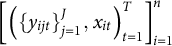 $ \left [ \left ( \left \{ y_{ijt}\right \}^J_{j=1}, \: x_{it} \right )^T_{t=1} \right ]^n_{i=1} $
.
$ \left [ \left ( \left \{ y_{ijt}\right \}^J_{j=1}, \: x_{it} \right )^T_{t=1} \right ]^n_{i=1} $
.
 $ x_{it} $
is a vector of observed, exogenous variables affecting
$ x_{it} $
is a vector of observed, exogenous variables affecting
 $ y^*_{ijt} $
. In words, for each person and each time period, we observe a set of explanatory variables
$ y^*_{ijt} $
. In words, for each person and each time period, we observe a set of explanatory variables
 $ x_{it} $
and a set of answers to the attitudes questions
$ x_{it} $
and a set of answers to the attitudes questions
 $ y_{ijt} $
. We model each latent attitude
$ y_{ijt} $
. We model each latent attitude
 $ j $
as
$ j $
as
 $$ \begin{align} y^*_{ijt} = x_{it} \: \beta_j + \delta_{jt} + \sum_{m=1}^M \lambda_{jm} \: e_{im} + u_{ijt}, \end{align} $$
where
 $ \delta _{jt} $
is a time- and-attitude-specific fixed effect,
$ \delta _{jt} $
is a time- and-attitude-specific fixed effect,
 $ e_{im} $
are unobserved time-invariant person-specific factors, and the
$ e_{im} $
are unobserved time-invariant person-specific factors, and the
 $ u_{ijt} $
shocks are jointly distributed.
$ u_{ijt} $
shocks are jointly distributed.
There are
 $ M $
uncorrelated factors
$ M $
uncorrelated factors
 $ \left \{ e_{im} \right \}_{m=1}^M $
, factor
$ \left \{ e_{im} \right \}_{m=1}^M $
, factor
 $ m $
for individual
$ m $
for individual
 $ i $
, and attitudes load on them using the
$ i $
, and attitudes load on them using the
 $ \lambda _{jm} $
coefficients, equivalent to a multivariate normal random effect. Setting
$ \lambda _{jm} $
coefficients, equivalent to a multivariate normal random effect. Setting
 $ M = 2 $
in both applications is flexible enough to capture substantial permanent attitudinal variation across the population. The inclusion of the factor loadings
$ M = 2 $
in both applications is flexible enough to capture substantial permanent attitudinal variation across the population. The inclusion of the factor loadings
 $ \lambda _{jm} $
means that the permanent person-specific effects can be correlated.
$ \lambda _{jm} $
means that the permanent person-specific effects can be correlated.
We employ a flexible shock structure. Denote by
 $ u_{it} $
the shocks to individual
$ u_{it} $
the shocks to individual
 $ i $
at time
$ i $
at time
 $ t $
across attitudes, i.e.,
$ t $
across attitudes, i.e.,
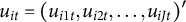 $ u_{it} = \left ( u_{i1t}, u_{i2t}, \dots , u_{iJt} \right )' $
. Let
$ u_{it} = \left ( u_{i1t}, u_{i2t}, \dots , u_{iJt} \right )' $
. Let
 $ u_i $
be all the shocks experienced by individual
$ u_i $
be all the shocks experienced by individual
 $ i $
for all attitudes and all time periods, i.e.,
$ i $
for all attitudes and all time periods, i.e.,
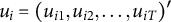 $ u_i = \left ( u_{i1}, u_{i2}, \dots , u_{iT} \right )' $
. Each individual’s shocks are distributed,
$ u_i = \left ( u_{i1}, u_{i2}, \dots , u_{iT} \right )' $
. Each individual’s shocks are distributed,
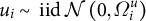 $ u_i \sim \text { iid } \mathcal {N}\left ( 0, \Omega _i^u \right ) $
. The covariance matrix
$ u_i \sim \text { iid } \mathcal {N}\left ( 0, \Omega _i^u \right ) $
. The covariance matrix
 $ \Omega _i^u $
is of size
$ \Omega _i^u $
is of size
 $ JT{\times }JT $
, and we fix all
$ JT{\times }JT $
, and we fix all
 $ \Omega ^u_{ittjj} = 1 $
, an assumption that normalizes units, common to all ordered discrete models.
$ \Omega ^u_{ittjj} = 1 $
, an assumption that normalizes units, common to all ordered discrete models.
The time between interviews varies across waves and people, making it inappropriate to assume that
 $ \Omega ^u_i $
is constant across individuals. We specify
$ \Omega ^u_i $
is constant across individuals. We specify
 $ \Omega ^u_i $
as
$ \Omega ^u_i $
as
 $$ \begin{align} \Omega_i^u = \begin{pmatrix} I & \Upsilon_{i12} & \Upsilon_{i13} & \dots & \Upsilon_{i1T} \\ \Upsilon_{i12} & I & \Upsilon_{i23} & \dots & \Upsilon_{i2T} \\ \Upsilon_{i13} & \Upsilon_{i23} & I & \dots & \Upsilon_{i3T} \\ \vdots & \vdots & \vdots & \ddots & \vdots \\ \Upsilon_{i1T} & \Upsilon_{i2T} & \Upsilon_{i3T} & \dots & I \end{pmatrix}, \end{align} $$
where the blocks on the main diagonal are identity matrices. All blocks are
 $ J{\times }J $
. Define
$ J{\times }J $
. Define
 $ \rho _{jk} $
as the effect of
$ \rho _{jk} $
as the effect of
 $ u_{ijt} $
on
$ u_{ijt} $
on
 $ u_{ikt'} $
for
$ u_{ikt'} $
for
 $ t' $
equal to some time after
$ t' $
equal to some time after
 $ t $
, and model the
$ t $
, and model the
 $ jk$
-element of
$ jk$
-element of
 $ \Upsilon _{itt'} $
as
$ \Upsilon _{itt'} $
as
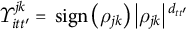 $ \Upsilon ^{jk}_{itt'} = \text { sign}\left ( \rho _{jk} \right ) \left | \rho _{jk} \right |{}^{d_{tt'}} $
, with
$ \Upsilon ^{jk}_{itt'} = \text { sign}\left ( \rho _{jk} \right ) \left | \rho _{jk} \right |{}^{d_{tt'}} $
, with
 $ d_{tt'} $
the time between
$ d_{tt'} $
the time between
 $ t $
and
$ t $
and
 $ t' $
.Footnote 12 This adjusts
$ t' $
.Footnote 12 This adjusts
 $ \Omega ^u_i $
across people and waves.
$ \Omega ^u_i $
across people and waves.
 $y^*_{ijt}$
is latent. It translates to the discrete choices in the data through
$y^*_{ijt}$
is latent. It translates to the discrete choices in the data through
 $$\begin{align*}y_{ijt} = k, \text{ if and only if } \tau_{kj} < y^*_{ijt} \le \tau_{k+1j}, \end{align*}$$
i.e., individual
 $ i $
chooses option
$ i $
chooses option
 $ k $
in response to survey question
$ k $
in response to survey question
 $ j $
in period
$ j $
in period
 $ t $
if and only if the latent attitude falls within an interval specific to option
$ t $
if and only if the latent attitude falls within an interval specific to option
 $ k $
. The probability that the individual reports
$ k $
. The probability that the individual reports
 $ y_{ijt} = k $
is the probability that
$ y_{ijt} = k $
is the probability that
 $ y^*_{ijt} $
is between
$ y^*_{ijt} $
is between
 $ \tau _{kj} $
and
$ \tau _{kj} $
and
 $ \tau _{k+1j} $
.
$ \tau _{k+1j} $
.
We use maximum simulated likelihood for estimation (Börsch-Supan and Hajivassiliou Reference Börsch-Supan and Hajivassiliou1993; Stern Reference Stern1997). We relegate our model’s estimation and implementation to Appendix A.1 of the Supplementary Material, including conditions for stationarity, data requirements, and computation time requirements.
3.2 Identification
To disentangle the joint evolution of attitudes and provide a causal interpretation, further identifying assumptions are necessary. Our model nests a (structural) vector autoregressive specification for shocks. Multiple identification schemes for such structures are available (Kilian and Lütkepohl Reference Kilian and Lütkepohl2017). We choose to achieve identification by restricting shocks to be uncorrelated contemporaneously across attitudes. We do allow, though, unrestricted spillovers across attitudes with a lag. This restriction is implemented through the imposition of identity matrices for the main diagonal of Equation (2). In practice, this means that we do not allow attitudes to exhibit contemporaneously correlated shocks, but that, following a shock to an attitude today, other attitudes' shocks can respond, either positively or negatively, after at least one time period. The lack of contemporaneous correlation in shocks is, in part, mitigated by the correlation in the unobserved time-invariant person-specific effects, which captures the time-invariant component of the correlation between shocks.
Other identifying schemes are possible. For example, if we hold strong, theory-informed prior beliefs that shocks to one attitude should impact a certain other attitude contemporaneously, and not vice versa, we could employ a “lower triangular,” Cholesky scheme, where the ordering of attitudes determines which attitudes can spill over immediately to others. We lack such strong priors and therefore find our assumption most appropriate for our applications. Alternative schemes would require appropriate alterations of the covariance in Equation (2) and little or no changes to the rest of the model.
3.3 Model Analytics and Visualization
We report all coefficient estimates for both applications in the Appendices B and C of the Supplementary Material, but results are better showcased via more concise summaries and figures. In Appendix A.3 of the Supplementary Material, we detail the implementation of variance decomposition, which computes the contribution of each model component to the variation of attitudes in the data. For example, we report how much of the variation in Trust in MPs, in the BESIP, is due to variation across permanent unobserved individual effects, versus how much of it comes from time-specific effects capturing key events in the UK. Appendix A.4 of the Supplementary Material describes IRFs, a standard way to visualize the dynamics of interrelated shocks over time (Kilian and Lütkepohl Reference Kilian and Lütkepohl2017). We plot the evolution of multiple attitudes following a one-time shock to one of them, allowing visual inspection of the persistence of shocks and the spillovers that characterize attitude systems.
3.4 Heterogeneous Effects
Appendix A.5 of the Supplementary Material tackles the possibility that effects are heterogeneous across subpopulations or subsamples. We implement Lagrange multiplier tests for both applications, which allows us to evaluate whether coefficients vary across subgroups, at low computational cost. For example, we reject the null hypothesis that coefficients are the same pre- and post-Brexit.
4 An Application to Core Political Attitudes
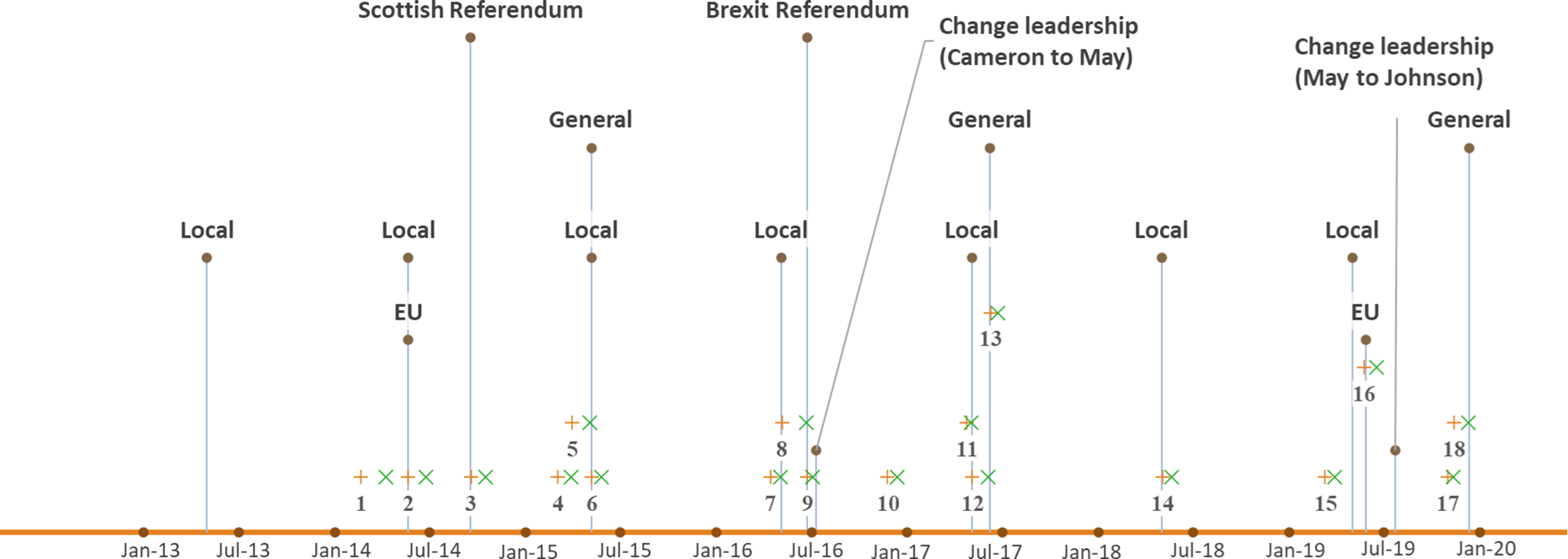
We use the BESIP (Fieldhouse et al. Reference Fieldhouse2024a,Reference Fieldhouseb) to assess the stability and constraint between five attitudes: the sense of civic duty to vote, people’s trust in Members of Parliament, internal political efficacy, external political efficacy, and satisfaction with how democracy is working in the UK. Appendix B.3 of the Supplementary Material discusses our rationale for examining these particular attitudes. BESIP is close to an ideal dataset as individuals are surveyed repeatedly and relatively frequently. We use a sample of 484,616 observations over
 $ 15 $
waves, 2014–2019,Footnote 13 a turbulent time for political attitudes: three general elections, six sets of local elections, two E.U. elections, two referendums, including “Brexit” in 2016, and two changes to the ruling party’s leadership.Footnote 14
$ 15 $
waves, 2014–2019,Footnote 13 a turbulent time for political attitudes: three general elections, six sets of local elections, two E.U. elections, two referendums, including “Brexit” in 2016, and two changes to the ruling party’s leadership.Footnote 14
We characterize stability in terms of the half-life of shocks, the time it takes an attitude to revert halfway to the individual’s average level following a shock. All attitudes have half-life estimates below five weeks, meaning that any unexpectedly stronger or weaker attitude returns quickly to the person’s baseline level. We find unexplained deviations to be short-lived and the transmission of shocks across attitudes generally small, with a much bigger role for wave-specific effects and infrequently-changing demographic characteristics, like age, party affiliation, or education. In short, people exhibit permanent level differences in their political attitudes, much of which is explained by infrequently changing observed characteristics. Time-specific effects, which shift everyone’s attitudes equally, play a notable role too, which is to be expected given two high-stakes referendums and several scandals during our sample (Anderson and Tverdova Reference Anderson and Tverdova2003; Banducci and Karp Reference Banducci and Karp2003; Bowler and Karp Reference Bowler and Karp2004; Feitosa Reference Feitosa2020; Galais and Blais Reference Galais and Blais2016; Hansen and Pedersen Reference Hansen and Pedersen2014; Kim Reference Kim2021; Mendelsohn and Cutler Reference Mendelsohn and Cutler2000; Schuck et al. Reference Schuck2013). We find a meaningful but limited scope for permanent differences across individuals, time-invariant unobserved heterogeneity, in particular, for Trust in MPs and Civic Duty to Vote. Drawing on previous research and the timeline of significant political events outlined in Table B1 in the Supplementary Material, we comment in Appendix B.9 of the Supplementary Material on possible sources of wave-specific effects and own shocks, to gain further insights into the factors influencing the stability of these attitudes.
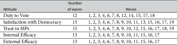
BESIP Data: Due to attrition and missing data, we use only between
 $ 12 $
and
$ 12 $
and
 $ 15 $
out of the
$ 15 $
out of the
 $ 19 $
waves for each attitude. Table 1 lists the waves used and Appendix B.4 of the Supplementary Material discusses BESIP’s strategies to manage panel attrition and conditioning. The resulting subset captures 86,816 respondents interviewed
$ 19 $
waves for each attitude. Table 1 lists the waves used and Appendix B.4 of the Supplementary Material discusses BESIP’s strategies to manage panel attrition and conditioning. The resulting subset captures 86,816 respondents interviewed
 $ 5.5 $
times on average, ample opportunity to observe repeatedly a large respondent pool. The sample covers multiple noteworthy developments associated by theory to changes in attitudes. Figure 1 illustrates the timing of waves and proximity to key events. A “
$ 5.5 $
times on average, ample opportunity to observe repeatedly a large respondent pool. The sample covers multiple noteworthy developments associated by theory to changes in attitudes. Figure 1 illustrates the timing of waves and proximity to key events. A “
 $ + $
” marks the beginning of each wave, while “
$ + $
” marks the beginning of each wave, while “
 $ \times $
” marks the end. The wave number is noted below each “
$ \times $
” marks the end. The wave number is noted below each “
 $+$
.” Events are marked using vertical lines. Controversial scandals are not plotted, but are listed in Table B1 in the Supplementary Material.
$+$
.” Events are marked using vertical lines. Controversial scandals are not plotted, but are listed in Table B1 in the Supplementary Material.
BESIP—Waves used for attitudes.

BESIP—Timeline of data collection and key elections.

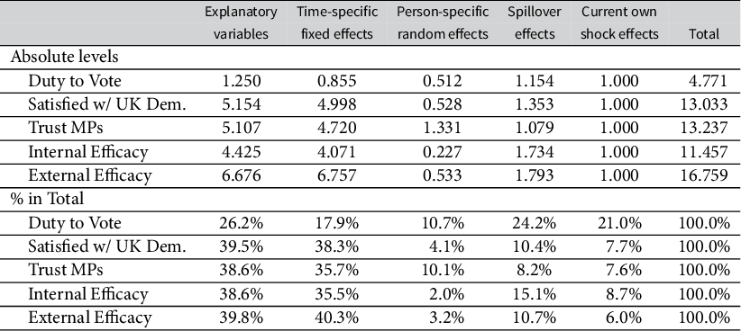
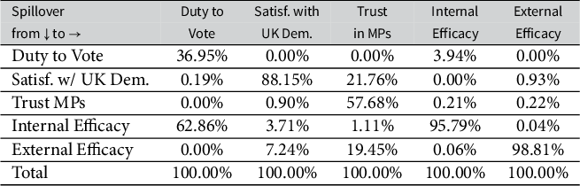
Findings: Table 2 reports the coefficient estimates for autocorrelations and spillovers across shocks (e.g., see the heatmap of Figure 2), Table 3 reports the variance decomposition, Table 4 outlines the relative influence of attitudes, while Table 5 reports the loadings of each attitude on the factors capturing time-invariant, unobserved heterogeneity. Figure 3 plots impulse responses, illustrating shocks’ dynamics. Appendix B.7 of the Supplementary Material discusses coefficients on observables, while other estimates and associated discussion are relegated to Appendices B.8, B.9, and B.10 of the Supplementary Material.
BESIP—Own persistence (
 $\rho _{jj}$
) and spillover coefficients (
$\rho _{jj}$
) and spillover coefficients (
 $\rho _{jk}$
).
$\rho _{jk}$
).

Note: Single-starred items are statistically significant at the 5% level. Standard errors are in parentheses.
 $ \rho $
estimates are restricted to be between
$ \rho $
estimates are restricted to be between
 $ (-1, 1) $
and are reported as monthly effects. Half-life standard errors are computed using the Delta Method. See the paragraph annotated with footnote 13 for further details.
$ (-1, 1) $
and are reported as monthly effects. Half-life standard errors are computed using the Delta Method. See the paragraph annotated with footnote 13 for further details.
BESIP—Variance decomposition.

BESIP—Relative attitude influence.

Note: Columns decompose the variance explained by shock-spillovers, “spillover variance,” by source attitude. Rows represent the sources of spillovers, one month after their respective own shocks.
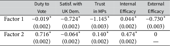
BESIP—Factor loadings on individual level random effects (
 $\lambda $
).
$\lambda $
).

Note: Single-starred items are statistically significant at the 5% level. Standard errors are in parentheses. The factor 2 loading for external efficacy is set to 0 as a normalization.
4.1 Attitude Stability
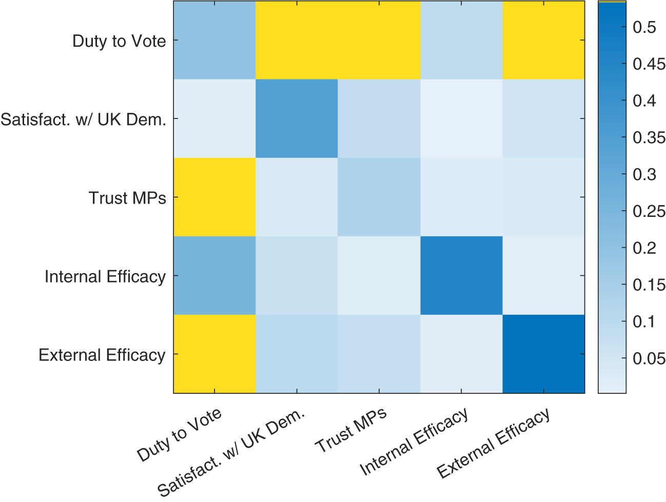
We evaluate each attitude’s resistance to both own and spillover shocks, the speed with which shocks decay. We decompose the variance of every attitude into proportions attributable to each model components. An attitude deemed stable is subject to highly transitory effects, from own and spillover shocks, and most of its variance is explained by time-invariant individual traits and infrequently-changing characteristics. The covariance of shocks, detailed in Table 2 and visualized in the heatmap Figure 2, summarizes the persistence of shocks.
The Persistence of Own Shocks: The main diagonal of Table 2 reports the autocorrelation of own shocks to each attitude. For example, the correlation between a shock to Internal Efficacy and the shock one month later is about
 $ 0.45 $
. Note that, because our shocks have unit variance, the covariances in Table 2 are correlations as well. These autocorrelations range from roughly
$ 0.45 $
. Note that, because our shocks have unit variance, the covariances in Table 2 are correlations as well. These autocorrelations range from roughly
 $ 0.13 $
for Trust in MPs, the least persistent, to about
$ 0.13 $
for Trust in MPs, the least persistent, to about
 $ 0.53 $
for External Efficacy, the most persistent. These are highly transitory shocks.
$ 0.53 $
for External Efficacy, the most persistent. These are highly transitory shocks.
Another way to interpret autocorrelations uses the half-life implied by
 $ \rho $
coefficients, via
$ \rho $
coefficients, via
 $ h_j = -\frac {\log 2}{\log \rho _{jj}} $
. The half-lives of shocks range from roughly one-third of a month, for Trust in MPs, to about a month, for External Efficacy. A quarter of the initial shock is expected after twice the half-life length, etc. The last row of Table 2 reports half-lives, and Delta Method standard errors.Footnote 15
$ h_j = -\frac {\log 2}{\log \rho _{jj}} $
. The half-lives of shocks range from roughly one-third of a month, for Trust in MPs, to about a month, for External Efficacy. A quarter of the initial shock is expected after twice the half-life length, etc. The last row of Table 2 reports half-lives, and Delta Method standard errors.Footnote 15
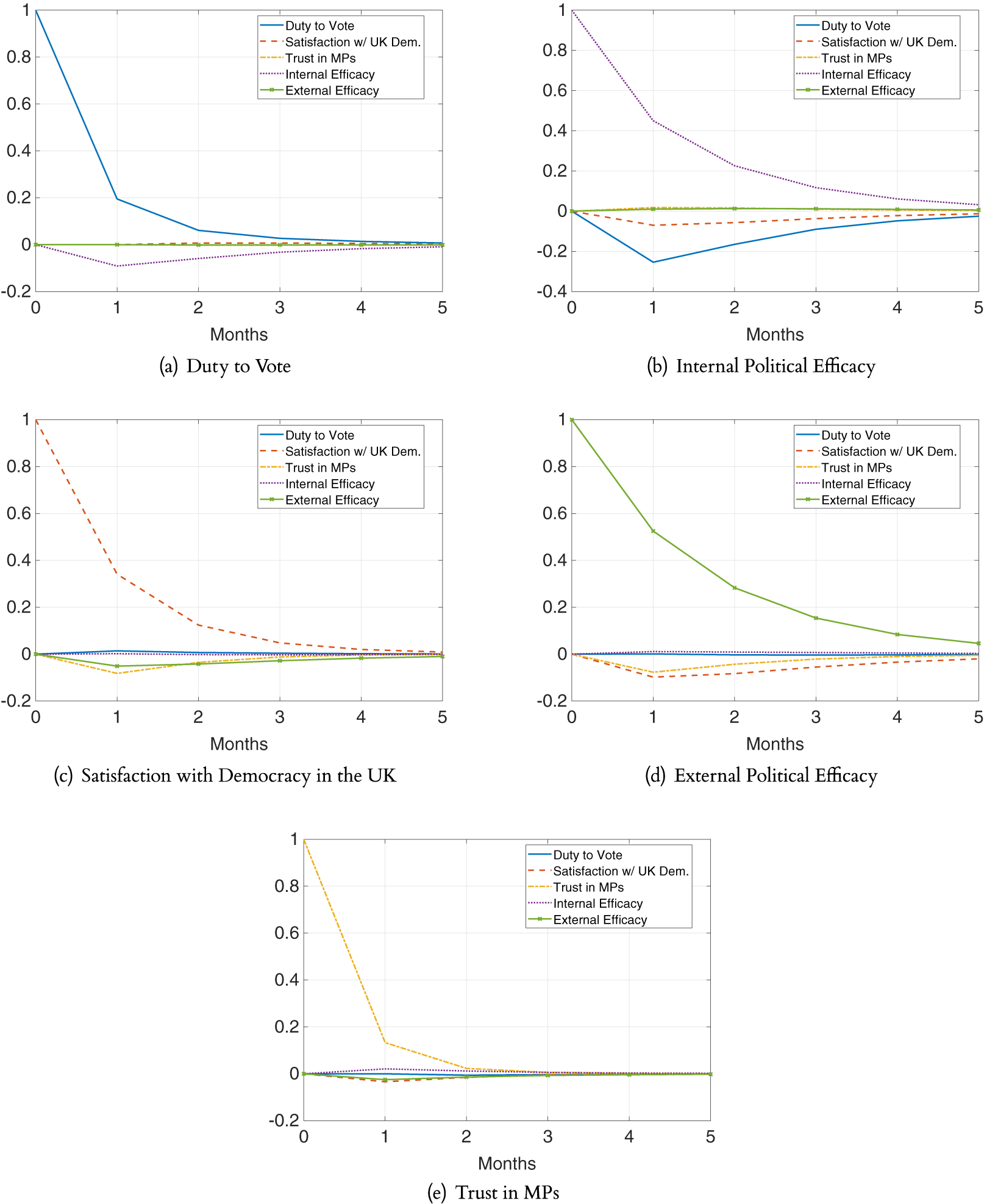
Figure 3 illustrates shocks via impulse responses. Each panel plots the evolution of all five shocks over time, following a one-time standard deviation (s.d.) increase in one of them.Footnote 16 Given our identification restriction, other shocks do not respond on impact, only the own shock increases by
 $ 1 $
. Following the initial impulse, all shocks are free to react with unrestricted sign. The most transitory shock is the one to Trust in MPs panel (e). For all practical purposes, the shock reverts to its baseline level within two months. This is similar for all attitudes, except External Efficacy panel (d), still modestly elevated five months after the initial impulse. In sum, shocks to latent attitudes are highly transitory; an idiosyncratically high attitude now is only weakly predictive of a higher value even a few weeks later.
$ 1 $
. Following the initial impulse, all shocks are free to react with unrestricted sign. The most transitory shock is the one to Trust in MPs panel (e). For all practical purposes, the shock reverts to its baseline level within two months. This is similar for all attitudes, except External Efficacy panel (d), still modestly elevated five months after the initial impulse. In sum, shocks to latent attitudes are highly transitory; an idiosyncratically high attitude now is only weakly predictive of a higher value even a few weeks later.
BESIP—Correlation heatmap of own (
 $|\rho _{jj}|$
) and spillover coefficients (
$|\rho _{jj}|$
) and spillover coefficients (
 $|\rho _{jk}|$
).
$|\rho _{jk}|$
).
Note: Coefficients are reported in absolute value, to ease comparison. Yellow cells denote correlations that are statistically insignificantly different from zero. Darker blue shades correspond to correlations that are larger in absolute value. The rows represent the source of the spillover effects.

BESIP—Impulse responses.
Note: Impulse response functions plot the dynamics over time of all attitudes, following a unit standard deviation shock to one of the attitudes, keeping fixed all other model components (i.e., observed explanatory variables, time and attitude specific fixed effects, and the individuals’ random factors).

Spillovers: Figure 3 also captures the spillovers of shocks. Using Internal Efficacy as an example, panel (b), the sequence of events is as follows: in month 0, a shock causes a unit standard deviation (s.d.) increase in Internal Efficacy. This induces spillovers to the other attitudes, one month later. At the one month mark, the spillovers are a
 $ 0.254 $
s.d. decrease in Civic Duty, a
$ 0.254 $
s.d. decrease in Civic Duty, a
 $ 0.07 $
s.d. decrease in Satisfaction with UK Democracy, a
$ 0.07 $
s.d. decrease in Satisfaction with UK Democracy, a
 $ 0.018 $
s.d. increase in Trust in MPs, and a
$ 0.018 $
s.d. increase in Trust in MPs, and a
 $ 0.01 $
s.d. increase in External Efficacy. The following month, month 2, there are new spillovers caused by (i) the initial, persistent own shock to Internal Efficacy and (ii) the spillovers from month 1. These dynamics continue indefinitely. In practice, due to small
$ 0.01 $
s.d. increase in External Efficacy. The following month, month 2, there are new spillovers caused by (i) the initial, persistent own shock to Internal Efficacy and (ii) the spillovers from month 1. These dynamics continue indefinitely. In practice, due to small
 $ \rho _{jk} $
estimates, effects become small quickly, indistinguishable from zero within months.
$ \rho _{jk} $
estimates, effects become small quickly, indistinguishable from zero within months.
Several takeaways are noteworthy. Spillovers are quantitatively modest, never exceeding
 $ \approx 0.3 $
s.d. in absolute value. They are transitory and fade monotonically. Finally, the spillovers reflects underlying attitude systems. For example, a positive shock to Duty to Vote is associated with a negative response in Internal Efficacy one month later, and vice versa, consistent with the factor loadings in Table 5, the permanent individual-level associations between attitudes. We expand on attitude systems in Section 4.3.
$ \approx 0.3 $
s.d. in absolute value. They are transitory and fade monotonically. Finally, the spillovers reflects underlying attitude systems. For example, a positive shock to Duty to Vote is associated with a negative response in Internal Efficacy one month later, and vice versa, consistent with the factor loadings in Table 5, the permanent individual-level associations between attitudes. We expand on attitude systems in Section 4.3.
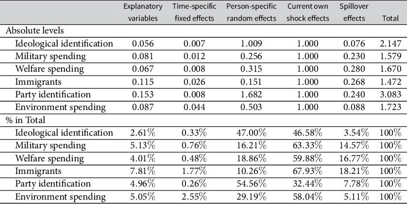
4.2 Variance Decomposition
So far, we discussed aspects of stability captured by the shocks. For a broader account, Table 3 reports the variance decomposition of Equation (1), in absolute levels and shares of total. Our model attributes latent
 $ y^*_{ijt} $
variation to several independent sources: infrequently-changing observable explanatory variables, time-specific effects, person-specific random effects, and shocks, either own or spillovers. Own shocks have unit variance by assumption, a normalization of the absolute levels, while spillovers are possible only with a lag, our identification restriction.
$ y^*_{ijt} $
variation to several independent sources: infrequently-changing observable explanatory variables, time-specific effects, person-specific random effects, and shocks, either own or spillovers. Own shocks have unit variance by assumption, a normalization of the absolute levels, while spillovers are possible only with a lag, our identification restriction.
Across attitudes,
 $ 25\% $
–
$ 25\% $
–
 $ 40\% $
of variance is due to infrequently-changing observed explanatory variables. A comparable share comes from time-specific effects, moving everyone’s attitudes together over time. The person-specific random effect contributes little, under
$ 40\% $
of variance is due to infrequently-changing observed explanatory variables. A comparable share comes from time-specific effects, moving everyone’s attitudes together over time. The person-specific random effect contributes little, under
 $ 11\% $
, a modest role for permanent unobserved heterogeneity across individuals. Shocks capture the rest, of which roughly half from own shocks. These findings hold across attitudes, with one exception: Duty to Vote is less sensitive to time effects, and more of its variance comes from shocks with about a quarter from spillovers. This captures the negative co-movement with Internal Efficacy, in Figure 3, when Internal Efficacy increases, Duty to Vote decreases slightly afterward.
$ 11\% $
, a modest role for permanent unobserved heterogeneity across individuals. Shocks capture the rest, of which roughly half from own shocks. These findings hold across attitudes, with one exception: Duty to Vote is less sensitive to time effects, and more of its variance comes from shocks with about a quarter from spillovers. This captures the negative co-movement with Internal Efficacy, in Figure 3, when Internal Efficacy increases, Duty to Vote decreases slightly afterward.
This decomposition reinforces the conclusion that attitudes are fairly stable at the individual level. Together, the time-invariant and infrequently-changing components of the model explain between
 $ 37\% $
and
$ 37\% $
and
 $ 49\% $
of the data. We treat the explanatory variables as stable because individuals seldom change education, income bins, or their party affiliation. The person-specific random effects explain little of the variance and capture permanent, unobserved heterogeneity. Finally, shocks are highly transitory; any deviation is effectively reverted within two months. On the other hand, one source of instability is possibly sizable: about a third of the variance is due to time-specific effects, common to all individuals.
$ 49\% $
of the data. We treat the explanatory variables as stable because individuals seldom change education, income bins, or their party affiliation. The person-specific random effects explain little of the variance and capture permanent, unobserved heterogeneity. Finally, shocks are highly transitory; any deviation is effectively reverted within two months. On the other hand, one source of instability is possibly sizable: about a third of the variance is due to time-specific effects, common to all individuals.
4.3 Constraint between Attitudes
We examine constraint in terms of spillovers, the relative influence of attitudes, and time-invariant individual traits.
Attitude Systems: The estimates reveal the presence of two attitude systems, as illustrated by the off-diagonal elements of Table 2, the correlation heatmap in Figure 2, and the shock spillovers in each panel of Figure 3. These systems are connected via Internal Efficacy and, to a lesser extent, Satisfaction with Democracy in the UK.
The first system captures how people view themselves as political actors, it consists of Civic Duty and Internal Efficacy. A one s.d. increase in Civic Duty results in a
 $ 0.09 $
s.d. decrease in Internal Efficacy, and this spillover persists for four months. In contrast, increases in Internal Efficacy have a relatively larger effect on Civic Duty. A
$ 0.09 $
s.d. decrease in Internal Efficacy, and this spillover persists for four months. In contrast, increases in Internal Efficacy have a relatively larger effect on Civic Duty. A
 $ 1 $
s.d. increase in Internal Efficacy causes a
$ 1 $
s.d. increase in Internal Efficacy causes a
 $ 0.25 $
s.d. decrease in Civic Duty, an effect of comparable persistence. Importantly, shocks to Civic Duty have no discernible spillovers to the other remaining three attitudes, while shocks to Internal Efficacy have only weak and short-lived effects.
$ 0.25 $
s.d. decrease in Civic Duty, an effect of comparable persistence. Importantly, shocks to Civic Duty have no discernible spillovers to the other remaining three attitudes, while shocks to Internal Efficacy have only weak and short-lived effects.
Another attitude system captures people’s evaluations of the external political world. It consists of Satisfaction with UK Democracy, External Efficacy, and Trust in MPs. Shocks to any of these result in decreases in the other two. Spillovers here are small, implying that attitudes are only weakly constrained. A one s.d. shock to Trust in MPs leads to a
 $ 0.025 $
s.d. decrease in External Efficacy and a
$ 0.025 $
s.d. decrease in External Efficacy and a
 $ 0.034 $
s.d. decrease in Satisfaction with UK Democracy. Spillovers from Trust in MPs continue to affect the other attitudes for about two months. Shocks to Satisfaction with UK Democracy and External Efficacy have larger and longer-lived spillovers, but even these decay within three months. Shocks from this system have no effect on Civic Duty and impact Internal Efficacy only weakly.
$ 0.034 $
s.d. decrease in Satisfaction with UK Democracy. Spillovers from Trust in MPs continue to affect the other attitudes for about two months. Shocks to Satisfaction with UK Democracy and External Efficacy have larger and longer-lived spillovers, but even these decay within three months. Shocks from this system have no effect on Civic Duty and impact Internal Efficacy only weakly.
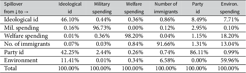
Relative Influence: Table 4 reports the decomposition of spillover variance, by source. Columns correspond to the attitudes that receive the spillovers, the rows are the sources. For example, the second column breaks down Civic Duty’s spillover variance, one month after each row attitude’s own shocks. The persistent effects of its own shock contribute
 $ 37\% $
and effects from Internal Efficacy explains
$ 37\% $
and effects from Internal Efficacy explains
 $ 62.9\% $
. The rest have no influence. Civic Duty and Internal Efficacy have the strongest influence on each other, with Internal Efficacy substantially more influential. External Efficacy receives modest spillovers. It is the most influential of the three attitudes capturing how people evaluate the external political world.
$ 62.9\% $
. The rest have no influence. Civic Duty and Internal Efficacy have the strongest influence on each other, with Internal Efficacy substantially more influential. External Efficacy receives modest spillovers. It is the most influential of the three attitudes capturing how people evaluate the external political world.
Unobserved Individual-Level Heterogeneity: Table 5 reports factor loadings. Consistent with the spillovers, Civic Duty and Internal Efficacy both have their highest loading on factor 2, time-invariant unobserved heterogeneity in how people view themselves as political actors. Both attitudes load in the same direction: people who tend to feel politically efficacious are also predisposed to believe that citizens have a duty to vote. The second system, the other three attitudes, loads the highest on factor 1, unobserved time-invariant heterogeneity in people’s evaluations of the external political world. Individuals with an innate tendency toward satisfaction with UK democracy are predisposed to higher levels of external efficacy and trust in MPs.
5 An Application to Symbolic Identifications and Issue Attitudes
We estimate our model on a smaller dataset, in terms of respondents and waves, closer to frequently used panels. We study party identification, ideological identification, and attitudes about immigration and government spending. We stress the relationships within and between symbolic identifications and issue attitudes. All attitudes form a single, weakly-constrained system. Party identification is the most influential, particularly through its impact on ideological identification. Both symbolic identifications induce small but statistically significant spillovers to issue attitudes. Party and ideological identifications are stable, most variance coming from infrequently-changing or time-invariant model components. The issue attitudes are unstable, explained mainly by transitory shocks. Drawing on prior research, we comment in Appendix C.3 of the Supplementary Material on changes in respondents’ consideration pool, differential item functioning, and random measurement error.
5.1 GSS Data
The GSS is a full-probability survey of non-institutionalized adults (Davern et al. Reference Davern, Bautista, Freese, Herd and Morgan2025). We stacked four rotating panels, to study six attitudes. Appendix C.1 of the Supplementary Material lists the survey questions, Table C.5 in the Supplementary Material reports descriptive statistics, and Appendix C.2 of the Supplementary Material summarizes our rationale for examining these attitudes. Appendix C.4 of the Supplementary Material discusses work examining panel conditioning and attrition for the GSS rotating panel.
The format of results mirrors the BESIP application. Table 6 compiles estimates of autocorrelations and spillovers (Figure 4 and 5). Table 7 reports variance decompositions, Table 8 the relative influence of attitudes, and Table 9 lists factor loadings for permanent unobserved heterogeneity. Figure 5 plots impulse responses. Remaining estimates are in Appendices C.8 and C.9 of the Supplementary Material.
GSS—Own persistence and spillover coefficients (
 $\rho _{jk}$
).
$\rho _{jk}$
).

Note: Single-starred items are statistically significant at the 5% level. Standard errors are in parentheses.
 $ \rho $
estimates are restricted to be between
$ \rho $
estimates are restricted to be between
 $ (-1, 1) $
and are reported as monthly effects. Half-life standard errors are computed using the Delta Method. See the paragraph annotated with footnote 13 for further details.
$ (-1, 1) $
and are reported as monthly effects. Half-life standard errors are computed using the Delta Method. See the paragraph annotated with footnote 13 for further details.
GSS—Variance decomposition.

GSS—Relative attitude influence.

Note: Columns decompose the variance explained by spillover-shocks (“spillover variance”) by source attitude. Rows represent the sources of shock-spillovers one month after their respective own-shocks.
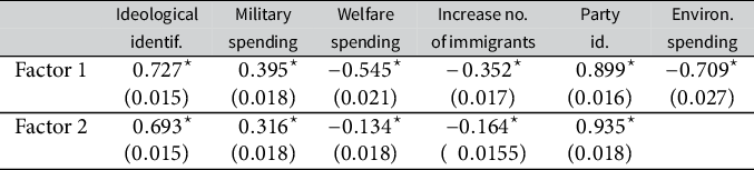
GSS—Factor loadings on individual level random effects (
 $\lambda $
).
$\lambda $
).

Note: Single-starred items are statistically significant at the 5% level. Standard errors are in parentheses. The factor 2 loading for environment spending is set to 0 as a normalization.
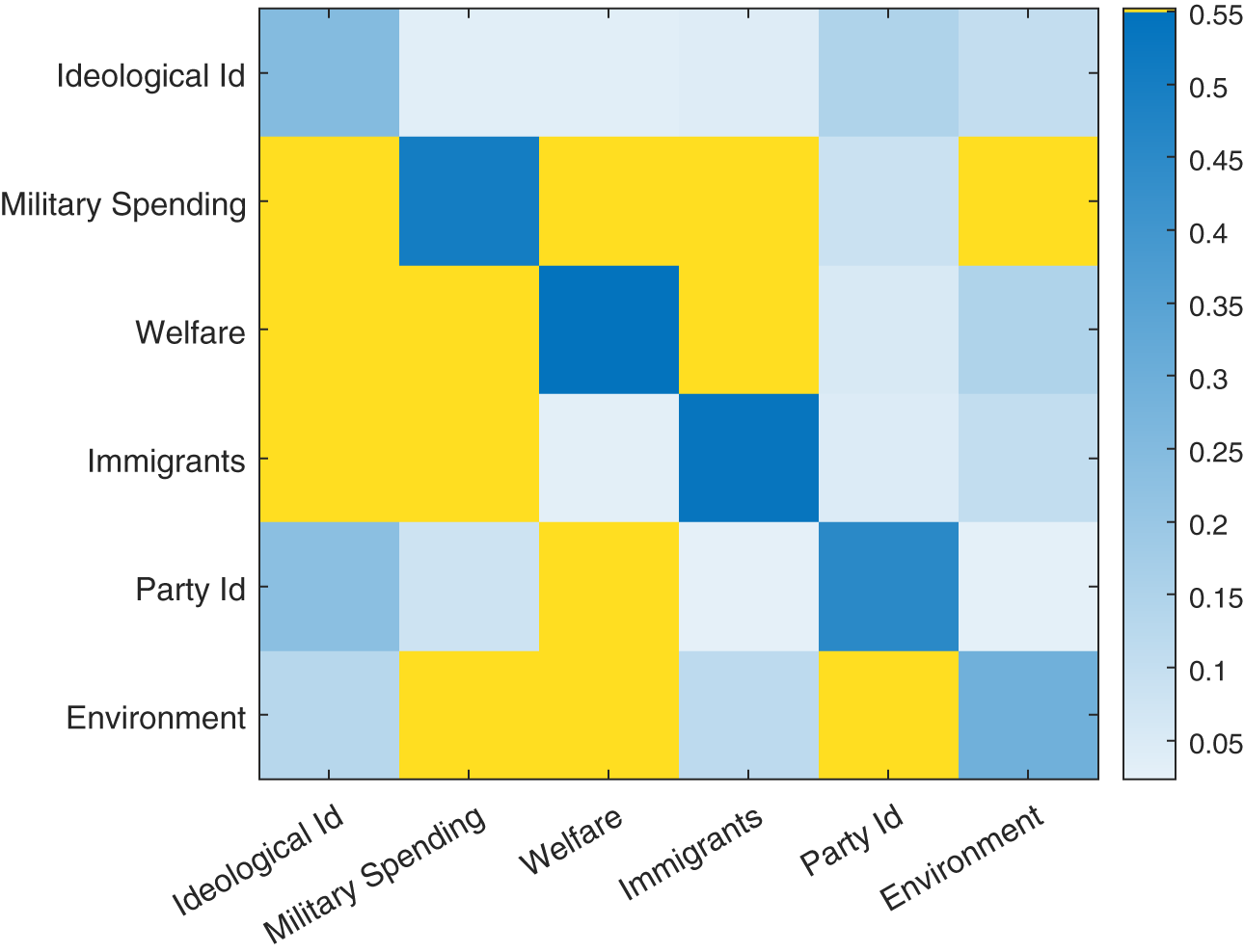
GSS—Correlation heatmap of own (
 $|\rho _{jj}|$
) and spillover coefficients (
$|\rho _{jj}|$
) and spillover coefficients (
 $|\rho _{jk}|$
).
$|\rho _{jk}|$
).
Note: Coefficients are reported in absolute value, to ease comparison. Yellow cells denote correlations that are statistically insignificantly different from zero. Darker blue shades correspond to correlations that are larger in absolute value. The rows represent the source of the spillover effects.

GSS—Impulse responses.

5.2 Stability and Variance Decomposition
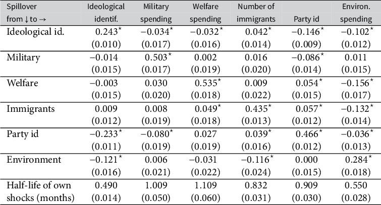
Based on Table 6 and Figure 5, shocks are transitory, with half-lives below
 $ 1.1 $
months. Ideological identification is the most transitory. Spillovers are modest, ranging from
$ 1.1 $
months. Ideological identification is the most transitory. Spillovers are modest, ranging from
 $ 0.001 $
to
$ 0.001 $
to
 $ -0.23 $
.
$ -0.23 $
.
Substantial variation in party (
 $ 59.5\% $
) and ideological identification (
$ 59.5\% $
) and ideological identification (
 $ 49.6\% $
) are explained by infrequently-changing observables and permanent, unobserved heterogeneity. This aligns with work on the important role of permanent characteristics and stable factors, e.g., core values (Alford, Funk, and Hibbing Reference Alford, Funk and Hibbing2005; Dawes and Fowler Reference Dawes and Fowler2009; Feldman Reference Feldman, Sears, Huddy and Jervis2003; Hatemi et al. Reference Hatemi2010; Jost Reference Jost2017; Jost, Nosek, and Gosling Reference Jost, Nosek and Gosling2008; Kandler, Bleidorn, and Riemann Reference Kandler, Bleidorn and Riemann2012; Niemi and Jennings Reference Niemi and Jennings1991; Smith et al. Reference Smith, Oxley, Hibbing, Alford and Hibbing2011). For both symbolic identifications, own shocks contribute the next highest proportion. Spillovers are small, and time-specific effects are negligible.
$ 49.6\% $
) are explained by infrequently-changing observables and permanent, unobserved heterogeneity. This aligns with work on the important role of permanent characteristics and stable factors, e.g., core values (Alford, Funk, and Hibbing Reference Alford, Funk and Hibbing2005; Dawes and Fowler Reference Dawes and Fowler2009; Feldman Reference Feldman, Sears, Huddy and Jervis2003; Hatemi et al. Reference Hatemi2010; Jost Reference Jost2017; Jost, Nosek, and Gosling Reference Jost, Nosek and Gosling2008; Kandler, Bleidorn, and Riemann Reference Kandler, Bleidorn and Riemann2012; Niemi and Jennings Reference Niemi and Jennings1991; Smith et al. Reference Smith, Oxley, Hibbing, Alford and Hibbing2011). For both symbolic identifications, own shocks contribute the next highest proportion. Spillovers are small, and time-specific effects are negligible.
Issue attitudes are unstable, most variance comes from volatile sources,
 $ 65.7\% $
–
$ 65.7\% $
–
 $ 81.9\% $
. The one concerning immigrants is the least stable, while environmental spending is the most stable. Transitory shocks and spillovers, and the large proportion of variance they explain,
$ 81.9\% $
. The one concerning immigrants is the least stable, while environmental spending is the most stable. Transitory shocks and spillovers, and the large proportion of variance they explain,
 $ 63.2\% $
–
$ 63.2\% $
–
 $ 86.1\% $
, suggest that shocks capture frequently-changing consideration pools (Zaller and Feldman Reference Zaller and Feldman1992), random measurement error, and issues of differential item functioning of survey instruments. This puts into question the extent to which members of the public hold true attitudes about these issues. Even if, in the best-case scenario, all shocks reflect changing consideration pools, the only source indicative of true attitude change, the transient nature of the shocks still suggests that the public is either easily and frequently persuaded by competing arguments or often engages in temporary expressive responding.
$ 86.1\% $
, suggest that shocks capture frequently-changing consideration pools (Zaller and Feldman Reference Zaller and Feldman1992), random measurement error, and issues of differential item functioning of survey instruments. This puts into question the extent to which members of the public hold true attitudes about these issues. Even if, in the best-case scenario, all shocks reflect changing consideration pools, the only source indicative of true attitude change, the transient nature of the shocks still suggests that the public is either easily and frequently persuaded by competing arguments or often engages in temporary expressive responding.
5.3 Constraint and Time-Invariant Unobserved Heterogeneity
All attitudes form a single, weakly constrained attitude system. Table 8 decomposes spillover variance. Party identification is the most influential, particularly, via spillovers to ideological identification, which explain
 $ 42.3\% $
of the spillover variance in ideology, comparable to ideological identification’s own shocks. This echoes the literature’s emphasis on the increasing association between party and ideological identification (Abramowitz and Saunders Reference Abramowitz and Saunders2006; Halliez and Thornton Reference Halliez and Thornton2021; Levendusky Reference Levendusky2009) and the growing importance of party identification (Bafumi and Shapiro Reference Bafumi and Shapiro2009; Bartels Reference Bartels2000). Party identification has a stronger influence on attitudes toward defense spending than ideological identification, which, in turn, has a stronger influence on attitudes toward immigration, welfare, and environmental spending. Issue attitudes have small but meaningful influence on each other, under
$ 42.3\% $
of the spillover variance in ideology, comparable to ideological identification’s own shocks. This echoes the literature’s emphasis on the increasing association between party and ideological identification (Abramowitz and Saunders Reference Abramowitz and Saunders2006; Halliez and Thornton Reference Halliez and Thornton2021; Levendusky Reference Levendusky2009) and the growing importance of party identification (Bafumi and Shapiro Reference Bafumi and Shapiro2009; Bartels Reference Bartels2000). Party identification has a stronger influence on attitudes toward defense spending than ideological identification, which, in turn, has a stronger influence on attitudes toward immigration, welfare, and environmental spending. Issue attitudes have small but meaningful influence on each other, under
 $ 19\% $
.
$ 19\% $
.
In Table 9, all attitudes except party identification load the strongest on factor 1, which represents both ideological identity and operational ideology. Given party identification’s sizable influence on ideological identification and military spending, we treat it as part of the same attitude system. Attitudes load as expected based on their partisan leaning. Ideological and party identification, coded with Conservatives and Republicans scoring higher, load in the same direction as increasing military spending, an issue historically associated with the Republican Party (Petrocik Reference Petrocik1996). The remaining three issue attitudes, which historically the Democratic party has championed, load in the opposite direction.
6 Conclusion
Our model opens several avenues for future work. It applies to many settings where multiple ordinal outcomes are studied with panel data and where questions of stability or co-evolution are salient. Methodologically, we provide a toolkit for the study of stability and constraint between attitudes measured using ordinal scales. It detects attitude systems, informs assessments of stability and influence, and illustrates attitudinal dynamics following identified shocks. Our results match previous findings, for example, the measured constraint between party and ideological identifications fits the emphasis on their growing association (Abramowitz and Saunders Reference Abramowitz and Saunders2006; Halliez and Thornton Reference Halliez and Thornton2021; Levendusky Reference Levendusky2009), and party identification’s stronger influence (Bafumi and Shapiro Reference Bafumi and Shapiro2009; Bartels Reference Bartels2000). We also report novel substantive findings, e.g., concerning the large role of unobserved permanent heterogeneity, and precise quantification of relationships discussed in the literature.
Supplementary Material
For supplementary material accompanying this paper, please visit https://doi.org/10.1017/pan.2026.10034.
Data Availability Statement
Replication data and code for both applications, together with detailed instructions, can be found in Harvard Dataverse: https://doi.org/10.7910/DVN/DUCHYS.
Acknowledgments
We are grateful to three anonymous reviewers and the editorial team at Political Analysis, Jason Barabas, Jennifer Jerit, Patrick Kraft, especially Gabriel Mihalache, Thomas Nelson, Ryan Vander Wielen, and Nicole Yadon, as well as participants at Political Psychology Workshop at The Ohio State University for their insightful comments and suggestions.
Author Contributions
Conceptualization: A.N., S.S.; Methodology: A.N., S.S.; Data curation: A.N., S.S.; Data visualization: A.N., S.S.; Writing original draft: A.N., S.S. Both authors approved the final submitted draft.
Competing Interests
The authors declare none.
Ethical Standards
The research meets all ethical guidelines, including adherence to the legal requirements of the study country.


 Open access