





Impact Statement
Detection of defects and identification of symptoms in monitoring industrial systems is a widely studied problem with applications in a large range of domains. In this article, we propose a novel method, dCAM, based on a convolutional neural network, dCNN, to detect precursors of anomalies in multivariate data series. Experiments with several synthetic datasets demonstrate that dCAM is more accurate than previous classification approaches and a viable solution for discriminant feature discovery and classification explanation in multivariate time series. We then experimentally evaluate our approach on a real and challenging use case dedicated to identifying vibration precursors on pumps in nuclear power plants.
1. Introduction
Massive collections of data series (or time series) are becoming a reality in virtually every scientific and social domain, and there is an increasingly pressing need for relevant applications to develop techniques that can efficiently analyze them (Palpanas, Reference Palpanas2015; Bagnall et al., Reference Bagnall, Cole, Palpanas and Zoumpatianos2019; Wang and Palpanas, Reference Wang and Palpanas2021; Jakovljevic et al., Reference Jakovljevic, Kostadinov, Aghasaryan, Palpanas, Benito, Cherifi, Cherifi, Moro, Rocha and Sales-Pardo2022). Data series anomaly detection is a crucial problem with applications in a wide range of fields (Palpanas, Reference Palpanas2015; Boniol et al., Reference Boniol, Paparrizos, Kang, Palpanas, Tsay, Elmore and Franklin2022; Paparrizos et al., Reference Paparrizos, Boniol, Palpanas, Tsay, Elmore and Franklin2022a, Reference Paparrizos, Kang, Boniol, Tsay, Palpanas and Franklin2022b), that all share the same well-studied goal (Barnet and Lewis, Reference Barnet and Lewis1994; Subramaniam et al., Reference Subramaniam, Palpanas, Papadopoulos, Kalogeraki and Gunopulos2006; Yeh et al., Reference Yeh, Zhu, Ulanova, Begum, Ding, Dau, Silva, Mueen and Keogh2016): detecting anomalies as fast as possible to avoid any critical event. Such applications can be found in biology, astronomy, and engineering areas. Some of these sectors are well-studied and theoretically well-explored. The knowledge acquired by the expert can be used to build an algorithm that efficiently detects any kind of behavior derived from a potential well-defined normality. However, such algorithms can be difficult to concretize and might have difficulty adapting to unknown or unclear changes over time. On the other side, if the data available are representative enough to correctly illustrate the system’s health state, a data-driven method could provide more flexibility. For instance, in the case of fraud detection, a knowledge-based model looks for known frauds, while a data-driven model might be helpful in finding new patterns, which is crucial since frauds can change frequently and dynamically. The same statement can be made in the general case of anomaly or outlier detection.
1.1. Anomaly detection primer
First, one should note that no single, universal definition of outliers or anomalies exists. In general, an anomaly is an observation that appears to deviate markedly from other members of the sample in which it occurs. This fact may raise suspicions that the specific observation was generated by a different mechanism than the remainder of the data. This mechanism may be an erroneous data measurement and collection procedure or an inherent variability in the domain of the data under inspection. Nevertheless, such observations are interesting in both cases, and the analyst would like to know about them. The latter can be tackled by either looking at single values or a sequence of points. In the specific context of points, we are interested in finding points that are far from the normal distribution of values that correspond to healthy states. In the specific context of sequences, we are interested in identifying anomalous subsequences that are, unlike an outlier, not a single abnormal value but rather an abnormal evolution of values. This work will study the specific case of subsequence anomaly detection in data series.
As usually addressed in the literature (Breunig et al., Reference Breunig, Kriegel, Ng and Sander2000; Keogh et al., Reference Keogh, Lonardi, Ratanamahatana, Wei, Lee and Handley2007; Liu et al., Reference Liu, Ting and Zhou2008; Liu et al., Reference Liu, Chen and Wang2009; Senin et al., Reference Senin, Lin, Wang, Oates, Gandhi, Boedihardjo, Chen and Frankenstein2015; Yeh et al., Reference Yeh, Zhu, Ulanova, Begum, Ding, Dau, Silva, Mueen and Keogh2016), one can decide to adopt a fully unsupervised method. These approaches benefit from working without needing any collection of known and tagged anomalies and can automatically detect unknown abnormal behaviors. Several approaches have been proposed. For example, general methods for multi-dimensional points outlier detection have been proposed (Breunig et al., Reference Breunig, Kriegel, Ng and Sander2000; Liu et al., Reference Liu, Ting and Zhou2008; Ma et al., Reference Ma, Ghojogh, Samad, Zheng and Crowley2020). Nevertheless, algorithms such as Isolation forest (Liu et al., Reference Liu, Ting and Zhou2008) seem to perform well for the specific case of subsequence anomaly detection (Boniol and Palpanas, Reference Boniol and Palpanas2020). Moreover, recently proposed approaches, such as NormA (Boniol et al., Reference Boniol, Linardi, Roncallo, Palpanas, Meftah and Remy2021) (that aims to build a weighted set of centroids summarizing the different recurrent subsequences in the data series) and Series2Graph (Boniol and Palpanas, Reference Boniol and Palpanas2020) (that aims to build a directed graph in which a trajectory corresponds to a subsequence in the time series), model the normal behaviors of the data series and have shown to outperform the previous state-of-the-art approaches.
1.2. Supervised detection of anomaly precursors
In the previous section, anomalies were considered unknown. However, one can assume that experts know precisely which event they want to detect and have a data series collection corresponding to these anomalies. In that case, we have a database of anomalies at our disposal. As a consequence, one can decide to adopt supervised methods. A question that naturally arises is the following: is it possible to detect subsequences that happened before the known anomaly that might lead to an explanation of the anomaly (and potentially predict it)? Such subsequences can be called precursors or symptoms of anomalies. Usually used in medical domains, we can infer the medical definition and adapt it to the task of anomaly detection in large data series. We will use the generic term precursors in the remainder of the article. Detecting such subsequences might be significantly helpful for knowledge experts to prevent future anomalies from occurring or understand why an anomaly occurred (or facilitate its understanding). In several engineering applications, it is required to analyze measurements from many sensors (across many different locations) to detect potential failures. Being able to detect failures is not enough, and identifying which sensors (and which timestamps) are related to the failure provides essential information on the origin of the failure. For instance, in the monitoring of nuclear power plants, it is as important to detect the vibration of a given pump as to identify precursors and unusual measurements of sensors within the plant that could explain or prevent future vibrations. Thus, the task is to detect (in a supervised manner) known anomalies and retrieve potential precursors. We now propose a formal definition of the problem mentioned above.
Problem 1 (Precursors Identification Problem Definition). Given a monitored system $ \mathcal{M} $
, a set of data series
$ \mathcal{M} $
, a set of data series $ {T}_{\mathcal{M}}^{\mathcal{N}} $
that represents the healthy state of
$ {T}_{\mathcal{M}}^{\mathcal{N}} $
that represents the healthy state of $ \mathcal{M} $
(healthy state labeled
$ \mathcal{M} $
(healthy state labeled $ \mathcal{N} $
), a set of data series
$ \mathcal{N} $
), a set of data series $ {T}_{\mathcal{M}}^{\mathcal{A}} $
that represents the state of
$ {T}_{\mathcal{M}}^{\mathcal{A}} $
that represents the state of $ \mathcal{M} $
before an anomalous state (anomalous state labeled
$ \mathcal{M} $
before an anomalous state (anomalous state labeled $ \mathcal{A} $
), we first have to find a function
$ \mathcal{A} $
), we first have to find a function $ f $
that takes as input
$ f $
that takes as input $ {T}_{\mathcal{M}}^{\mathcal{A}} $
and
$ {T}_{\mathcal{M}}^{\mathcal{A}} $
and $ {T}_{\mathcal{M}}^{\mathcal{N}} $
, and returns
$ {T}_{\mathcal{M}}^{\mathcal{N}} $
, and returns $ s\in \left\{\mathcal{N},\mathcal{A}\right\} $
. We then have to find a function
$ s\in \left\{\mathcal{N},\mathcal{A}\right\} $
. We then have to find a function $ g $
that takes as input
$ g $
that takes as input $ {T}_{\mathcal{M}}^{\mathcal{A}} $
and
$ {T}_{\mathcal{M}}^{\mathcal{A}} $
and $ f $
, and returns
$ f $
, and returns $ S\subset {T}_{\mathcal{M}}^{\mathcal{A}} $
(
$ S\subset {T}_{\mathcal{M}}^{\mathcal{A}} $
( $ S $
being the set of subsequences in
$ S $
being the set of subsequences in $ {T}_{\mathcal{M}}^{\mathcal{A}} $
precursors of the upcoming anomalies). Formally,
$ {T}_{\mathcal{M}}^{\mathcal{A}} $
precursors of the upcoming anomalies). Formally, $ f $
and
$ f $
and $ g $
can be written as follows:
$ g $
can be written as follows: $ f:{T}_{\mathcal{M}}^{\mathcal{N}},{T}_{\mathcal{M}}^{\mathcal{A}}\to \left\{\mathcal{N},\mathcal{A}\right\} $
and
$ f:{T}_{\mathcal{M}}^{\mathcal{N}},{T}_{\mathcal{M}}^{\mathcal{A}}\to \left\{\mathcal{N},\mathcal{A}\right\} $
and $ g:{T}_{\mathcal{M}}^{\mathcal{A}},\hskip0.5em f\to S $
.
$ g:{T}_{\mathcal{M}}^{\mathcal{A}},\hskip0.5em f\to S $
.
As Problem 1 is defined as a supervised task, one can decide to use time series classification approaches. The latter can be performed using either (1) pre-extracted features or (2) raw values of the time series.
For the first category (1), the main idea is to use the dataset of time series (or subsequences of time series) to create a dataset whose samples are described by features common to all-time series. For the specific case of time series, the feature extraction step can be performed using TSFresh Python library (Christ et al., Reference Christ, Braun, Neuffer and Kempa-Liehr2018) (Time Series Feature extraction based on scalable hypothesis tests). The latter is used for automated time series feature extraction and selection based on the FRESH algorithm (Christ et al., Reference Christ, Kempa-Liehr and Feindt2016). More specifically, it automatically selects relevant features for a specific task. This is achieved using statistical tests, time series heuristics, and machine learning algorithms. Then, using the feature-based dataset, standard machine learning classifiers can be employed to classify each time series. Examples of traditional machine learning classifiers are Support Vector Classifier (SVC) (Boser et al., Reference Boser, Guyon and Vapnik1992) (i.e., classifiers that map instances in space in order to maximize the width of the gap between the classes), naive Bayes classifier (Zhang, Reference Zhang2004) (i.e., classifiers based on Bayes’ theorem to predict the class of a new instance based on prior probabilities and class-conditional probabilities), Multi-Layer Perceptron (MLP) (Hinton, Reference Hinton1989) (i.e., fully connected neural networks), AdaBoost (Freund and Schapire, Reference Freund and Schapire1995) (i.e., boosting ensemble machine learning algorithms), or Random Forest Classifier (Ho, Reference Ho1995) (ensemble machine learning algorithm that combines multiple decision trees, where each tree is built using a random subset of the features and a random sample of the data). On top of the aforementioned classifiers, explainability frameworks, such as LIME (Ribeiro et al., Reference Ribeiro, Singh and Guestrin2016) and SHAP (Lundberg and Lee, Reference Lundberg and Lee2017) can be used in order to identify which features have the most important effect on the classification prediction. However, feature-based classification and explanation methods can be limited when applied to time series. Whereas features are efficient for summarizing time series datasets (e.g., setting a constant number of features for variable length time series), it might miss important information in the shape of consecutive values, which may be crucial for anomaly detection and precursor identification. Moreover, the choice of features heavily impacts the classification accuracy and is not desirable in tasks related to precursors identification with unknown properties. Therefore, using methods that do not need any feature selection step is preferable when working on agnostic scenarios.
For methods based on raw values of the time series (ii), standard data series classification methods are based on distances to the instances’ nearest neighbors, with k-NN classification (using the Euclidean or Dynamic Time Warping (DTW) distances) being a popular baseline method (Dau et al., Reference Dau, Bagnall, Kamgar, Yeh, Zhu, Gharghabi, Ratanamahatana and Keogh2019). Nevertheless, recent works have shown that ensemble methods using more advanced classifiers achieve better performance (Bagnall et al., Reference Bagnall, Lines, Hills and Bostrom2015; Lines et al., Reference Lines, Taylor and Bagnall2016). Following recent breakthroughs in the computer vision community, new studies successfully propose deep learning methods for data series classification (Chen et al., Reference Chen, Tang, Tino and Yao2013; Zheng et al., Reference Zheng, Liu, Chen, Ge and Zhao2014; Cui et al., Reference Cui, Chen and Chen2016; Le Guennec et al., Reference Le Guennec, Malinowski and Tavenard2016; Zhao et al., Reference Zhao, Lu, Chen, Liu and Wu2017; Wang et al., Reference Wang, Wang, Li and Wu2018; Fawaz et al., Reference Fawaz, Forestier, Weber, Idoumghar and Muller2019), such as Convolutional Neural Network (CNN) and Residual Neural Network (ResNet) (Wang et al., Reference Wang, Yan and Oates2017). For some CNN-based models, the Class Activation Map (CAM) (Zhou et al., Reference Zhou, Khosla, Oliva and Torralba2016) can be used as an explanation for the classification result. CAM has been used for highlighting the parts of an image that contribute the most to a given class prediction and has also been adapted to data series (Wang et al., Reference Wang, Yan and Oates2017; Fawaz et al., Reference Fawaz, Forestier, Weber, Idoumghar and Muller2019). Thus, CAM can be used to identify subsequences that contribute the most to the anomaly prediction and, consequently, to solve Problem 1. This article considers Convolutional Neural Network joined with the Class Activation Map as a strong baseline.
1.3. Limitations of previous approaches
As regards existing methods that can solve Problem 1, CNN/CAM for data series suffers from one important limitation. CAM is a weighted mapping technique that returns a univariate series (of the same length as the input instances) with high values aligned with the subsequences of the input that contribute the most to a given class identification. Thus, in the case of multivariate data series as input, no information can be retrieved from CAM on which dimension is contributing. Therefore, precursors within specific dimensions cannot be retrieved using existing methods.
1.4. Contributions
In this article, we will focus on solving Problem 1. First, we explore the possibility of using a supervised time series classification algorithm to solve precursor discovery tasks. We then propose a novel method, dCNN/dCAM, that overcomes the limitations of previous supervised algorithms. Moreover, dCNN/dCAM permits the identification of specific patterns (without any prior knowledge) and alerts the expert on the imminent occurrence of the anomaly. Finally, we demonstrate this latter claim in a real industrial use case. The article is structured as follows:
-
• Section 2: We first describe the notations and the concepts related to time series and neural networks. We then describe the usual Class Activation Map and explain its limitations regarding multivariate data series in detail.
-
• Section 3: We describe a new convolutional architecture, dCNN, that enables the comparison of dimensions by changing the structure of the network input and using two-dimensional convolutional layers. We then introduce dCAM, a novel method that takes advantage of dCNN and returns a multivariate CAM that identifies the important parts of the input series for each dimension.
-
• Section 4 : We then experimentally evaluate the classification accuracy of dCNN/dCAM over CNN/CAM on a synthetic benchmark and demonstrate the benefit of our proposed approach.
-
• Section 5 : We experimentally evaluate our proposed approach over a real industrial use case.
2. Background and related work
[Data Series] A multivariate, or D-dimensional data series $ T\in {\mathrm{\mathbb{R}}}^{\left(D,n\right)} $
is a set of
$ T\in {\mathrm{\mathbb{R}}}^{\left(D,n\right)} $
is a set of $ D $
univariate data series of length
$ D $
univariate data series of length $ n $
. We note
$ n $
. We note $ T=\left[{T}^{(0)},\dots, {T}^{\left(D-1\right)}\right] $
and for
$ T=\left[{T}^{(0)},\dots, {T}^{\left(D-1\right)}\right] $
and for $ j\in \left[0,D-1\right] $
, we note the univariate data series
$ j\in \left[0,D-1\right] $
, we note the univariate data series $ {T}^{(j)}=\left[{T}_0^{(j)},{T}_1^{(j)},\dots, {T}_{n-1}^{(j)}\right] $
. A subsequence
$ {T}^{(j)}=\left[{T}_0^{(j)},{T}_1^{(j)},\dots, {T}_{n-1}^{(j)}\right] $
. A subsequence $ {T}_{i,\mathrm{\ell}}^{(j)}\in {\mathrm{\mathbb{R}}}^{\mathrm{\ell}} $
of the dimension
$ {T}_{i,\mathrm{\ell}}^{(j)}\in {\mathrm{\mathbb{R}}}^{\mathrm{\ell}} $
of the dimension $ {T}^{(j)} $
of the multivariate data series
$ {T}^{(j)} $
of the multivariate data series $ T $
is a subset of contiguous values from
$ T $
is a subset of contiguous values from $ {T}^{(j)} $
of length
$ {T}^{(j)} $
of length $ \mathrm{\ell} $
(usually
$ \mathrm{\ell} $
(usually $ \mathrm{\ell}\ll n $
) starting at position
$ \mathrm{\ell}\ll n $
) starting at position $ i $
; formally,
$ i $
; formally, $ {T}_{i,\mathrm{\ell}}^{(j)}=\left[{T}_i^{(j)},{T}_{i+1}^{(j)},\dots, {T}_{i+\mathrm{\ell}-1}^{(j)}\right] $
.
$ {T}_{i,\mathrm{\ell}}^{(j)}=\left[{T}_i^{(j)},{T}_{i+1}^{(j)},\dots, {T}_{i+\mathrm{\ell}-1}^{(j)}\right] $
.
[Neural Network Notations] We are interested in classifying data series using a neural network architecture model. We define the neural network input as $ X\in {\mathrm{\mathbb{R}}}^n $
for univariate data series (with
$ X\in {\mathrm{\mathbb{R}}}^n $
for univariate data series (with $ {x}_i $
the
$ {x}_i $
the $ {i}^{th} $
value and
$ {i}^{th} $
value and $ {X}_{i,\mathrm{\ell}} $
the sequence of
$ {X}_{i,\mathrm{\ell}} $
the sequence of $ \mathrm{\ell} $
values following the
$ \mathrm{\ell} $
values following the $ {i}^{th} $
value), and
$ {i}^{th} $
value), and $ \mathbf{X}\in {\mathrm{\mathbb{R}}}^{\left(D,n\right)} $
for multivariate data series (with
$ \mathbf{X}\in {\mathrm{\mathbb{R}}}^{\left(D,n\right)} $
for multivariate data series (with $ {x}_{j,i} $
the
$ {x}_{j,i} $
the $ {i}^{th} $
value on the
$ {i}^{th} $
value on the $ {j}^{th} $
dimension and
$ {j}^{th} $
dimension and $ {\mathbf{X}}_{j,i,\mathrm{\ell}} $
the sequence of
$ {\mathbf{X}}_{j,i,\mathrm{\ell}} $
the sequence of $ \mathrm{\ell} $
values following the
$ \mathrm{\ell} $
values following the $ {i}^{th} $
value on the
$ {i}^{th} $
value on the $ {j}^{th} $
dimension).
$ {j}^{th} $
dimension).
Dense Layer: The basic layer of neural networks is a fully connected layer (also called $ \mathrm{dense} $ $ \mathrm{layer} $
) in which every input neuron is weighted and summed before passing through an activation function. For univariate data series, given an input data series
$ \mathrm{layer} $
) in which every input neuron is weighted and summed before passing through an activation function. For univariate data series, given an input data series $ X\in {\mathrm{\mathbb{R}}}^n $
, given a vector of weights
$ X\in {\mathrm{\mathbb{R}}}^n $
, given a vector of weights $ W\in {\mathrm{\mathbb{R}}}^n $
and a vector
$ W\in {\mathrm{\mathbb{R}}}^n $
and a vector $ B\in {\mathrm{\mathbb{R}}}^n $
, we have:
$ B\in {\mathrm{\mathbb{R}}}^n $
, we have:
 $ {f}_a $
is called the activation function and is a nonlinear function. The commonly used activation function
$ {f}_a $
is called the activation function and is a nonlinear function. The commonly used activation function $ {f}_a $
is the rectified linear unit (ReLU) (Nair and Hinton, Reference Nair and Hinton2010) that prevents the saturation of the gradient (other functions that have been proposed are Tanh and Leaky ReLU (Xu et al., Reference Xu, Wang, Chen and Li2015)). For the specific case of multivariate data series, all dimensions are concatenated to give input
$ {f}_a $
is the rectified linear unit (ReLU) (Nair and Hinton, Reference Nair and Hinton2010) that prevents the saturation of the gradient (other functions that have been proposed are Tanh and Leaky ReLU (Xu et al., Reference Xu, Wang, Chen and Li2015)). For the specific case of multivariate data series, all dimensions are concatenated to give input  . Finally, one can decide to have several output neurons. In this case, each neuron is associated with a different $ W $
and
$ W $
and $ B $
, and equation (1) is executed independently.
$ B $
, and equation (1) is executed independently.
Convolutional Layer: This layer has played a significant role in image classification (Krizhevsky et al., Reference Krizhevsky, Sutskever and Hinton2012; LeCun et al., Reference LeCun, Bengio and Hinton2015; Wang et al., Reference Wang, Yan and Oates2017), and recently for data series classification (Fawaz et al., Reference Fawaz, Forestier, Weber, Idoumghar and Muller2019). Formally, for multivariate data series, given an input vector $ \mathbf{X}\in {\mathrm{\mathbb{R}}}^{\left(D,n\right)} $
, and given matrices weights
$ \mathbf{X}\in {\mathrm{\mathbb{R}}}^{\left(D,n\right)} $
, and given matrices weights $ \mathbf{W},\mathbf{B}\in {\mathrm{\mathbb{R}}}^{\left(D,\mathrm{\ell}\right)} $
, the output
$ \mathbf{W},\mathbf{B}\in {\mathrm{\mathbb{R}}}^{\left(D,\mathrm{\ell}\right)} $
, the output $ h\in {\mathrm{\mathbb{R}}}^n $
of a convolutional layer can be seen as a univariate data series. The tuple
$ h\in {\mathrm{\mathbb{R}}}^n $
of a convolutional layer can be seen as a univariate data series. The tuple $ \left(W,B\right) $
is also called a kernel, with
$ \left(W,B\right) $
is also called a kernel, with $ \left(D,\mathrm{\ell}\right) $
the size of the kernel. Formally, for
$ \left(D,\mathrm{\ell}\right) $
the size of the kernel. Formally, for $ h=\left[{h}_0,\dots, {h}_n\right] $
, we have:
$ h=\left[{h}_0,\dots, {h}_n\right] $
, we have:

In practice, we have several kernels of size $ \left(D,\mathrm{\ell}\right) $
. The result is a multivariate series with dimensions equal to the number of kernels,
$ \left(D,\mathrm{\ell}\right) $
. The result is a multivariate series with dimensions equal to the number of kernels, $ {n}_f $
. For a given input
$ {n}_f $
. For a given input $ \mathbf{X}\in {\mathrm{\mathbb{R}}}^{\left(D,n\right)} $
, we define
$ \mathbf{X}\in {\mathrm{\mathbb{R}}}^{\left(D,n\right)} $
, we define $ A\in {\mathrm{\mathbb{R}}}^{\left({n}_f,n\right)} $
to be the output of a convolutional layer
$ A\in {\mathrm{\mathbb{R}}}^{\left({n}_f,n\right)} $
to be the output of a convolutional layer $ \mathrm{conv}\left({n}_f,\mathrm{\ell}\right) $
.
$ \mathrm{conv}\left({n}_f,\mathrm{\ell}\right) $
. $ {A}_m $
is thus a univariate series corresponding to the output of the
$ {A}_m $
is thus a univariate series corresponding to the output of the $ {m}^{th} $
kernel. We denote with
$ {m}^{th} $
kernel. We denote with $ {A}_m(T) $
the univariate series corresponding to the output of the
$ {A}_m(T) $
the univariate series corresponding to the output of the $ {m}^{th} $
kernel when
$ {m}^{th} $
kernel when $ T $
is used as input.
$ T $
is used as input.
Global Average Pooling Layer: Another type of layer frequently used is pooling. Pooling layers compute average/max/min operations, aggregating values of previous layers into a smaller number of values for the next layer. A specific type of pooling layer is Global Average Pooling (GAP). This operation averages an entire output of a convolutional layer $ {A}_m(T) $
into one value, thus providing invariance to the position of the discriminative features.
$ {A}_m(T) $
into one value, thus providing invariance to the position of the discriminative features.
Learning Phase: The learning phase uses a loss function $ \mathrm{\mathcal{L}} $
that measures the accuracy of the model and optimizes the various weights. For the sake of simplicity, we note
$ \mathrm{\mathcal{L}} $
that measures the accuracy of the model and optimizes the various weights. For the sake of simplicity, we note $ \Omega $
the set containing all weights (e.g., matrices
$ \Omega $
the set containing all weights (e.g., matrices $ \mathbf{W} $
and
$ \mathbf{W} $
and $ \mathbf{B} $
defined in the previous sections). Given a set of instances
$ \mathbf{B} $
defined in the previous sections). Given a set of instances $ \mathcal{X} $
, we define the average loss as:
$ \mathcal{X} $
, we define the average loss as: $ J\left(\Omega \right)=\frac{1}{\mid \mathcal{X}\mid }{\sum}_{\mathbf{X}\in \mathcal{X}}\mathrm{\mathcal{L}}\left(\mathbf{X}\right) $
. Then for a given learning rate
$ J\left(\Omega \right)=\frac{1}{\mid \mathcal{X}\mid }{\sum}_{\mathbf{X}\in \mathcal{X}}\mathrm{\mathcal{L}}\left(\mathbf{X}\right) $
. Then for a given learning rate $ \alpha $
, the average loss is back-propagated to all weights in the different layers. Formally, back-propagation is defined as follows:
$ \alpha $
, the average loss is back-propagated to all weights in the different layers. Formally, back-propagation is defined as follows: $ \forall \omega \in \Omega, \omega \leftarrow \omega -\alpha \frac{\partial J}{\partial \omega } $
. In this article, we use the stochastic gradient descent using the ADAM optimizer (Kingma and Ba, Reference Kingma and Ba2015) and cross-entropy loss function.
$ \forall \omega \in \Omega, \omega \leftarrow \omega -\alpha \frac{\partial J}{\partial \omega } $
. In this article, we use the stochastic gradient descent using the ADAM optimizer (Kingma and Ba, Reference Kingma and Ba2015) and cross-entropy loss function.
2.1. Convolutional-based neural network
We now describe the standard architectures used in the literature. The first is Convolutional Neural Networks (CNNs) (Wang et al., Reference Wang, Yan and Oates2017; Fawaz et al., Reference Fawaz, Forestier, Weber, Idoumghar and Muller2019). CNN is a concatenation of convolutional layers (joined with ReLU activation functions and batch normalization). The last convolutional layer is connected to a Global Average Pooling layer and a dense layer. In theory, instances of multiple lengths can be used with the same network. A second architecture is the Residual Neural Network (ResNet) (Wang et al., Reference Wang, Yan and Oates2017; Fawaz et al., Reference Fawaz, Forestier, Weber, Idoumghar and Muller2019). This architecture is based on the classical CNN, to which we add residual connections between successive blocks of convolutional layers to prevent the gradients from exploding or vanishing. Other methods have been proposed in the literature (Cui et al., Reference Cui, Chen and Chen2016; Serrà et al., Reference Serrà, Pascual and Karatzoglou2018; Fawaz et al., Reference Fawaz, Forestier, Weber, Idoumghar and Muller2019; Ismail Fawaz et al., Reference Ismail Fawaz, Lucas, Forestier, Pelletier, Schmidt, Weber, Webb, Idoumghar, Muller and Petitjean2020), though CNN and ResNet have been shown to perform the best for multivariate time series classification (Fawaz et al., Reference Fawaz, Forestier, Weber, Idoumghar and Muller2019). InceptionTime (Ismail Fawaz et al., Reference Ismail Fawaz, Lucas, Forestier, Pelletier, Schmidt, Weber, Webb, Idoumghar, Muller and Petitjean2020) has not been evaluated on multivariate data series but demonstrated state-of-the-art performance on univariate data series.
2.2. Class activation map
Once the model is trained, we need to find the discriminative features that led the model to decide which class to attribute to each instance. Class Activation Map (Zhou et al., Reference Zhou, Khosla, Oliva and Torralba2016) (CAM) has been proposed to highlight the parts of an image that contributes the most to a given class identification. The latter has been experimented on data series (Wang et al., Reference Wang, Yan and Oates2017; Fawaz et al., Reference Fawaz, Forestier, Weber, Idoumghar and Muller2019) (univariate and multivariate). This method explains the classification of a certain deep learning model by emphasizing the subsequences that contribute the most to a certain classification. Note that the CAM method can only be used if (1) a Global Average Pooling layer has been used before the softmax classifier, and (2) the model accuracy is high enough. Thus, only the standard architectures CNN and ResNet proposed in the literature can benefit from CAM. We now define the CAM method (Wang et al., Reference Wang, Yan and Oates2017; Fawaz et al., Reference Fawaz, Forestier, Weber, Idoumghar and Muller2019). For an input data series $ T $
, let
$ T $
, let $ A(T) $
be the result of the last convolutional layer
$ A(T) $
be the result of the last convolutional layer $ \mathrm{conv}\left({n}_f,\mathrm{\ell}\right) $
, which is a multivariate data series with
$ \mathrm{conv}\left({n}_f,\mathrm{\ell}\right) $
, which is a multivariate data series with $ {n}_f $
dimensions and of length
$ {n}_f $
dimensions and of length $ n $
.
$ n $
. $ {A}_m(T) $
is the univariate time series for the dimension
$ {A}_m(T) $
is the univariate time series for the dimension $ m\in \left[1,{n}_f\right] $
corresponding to the
$ m\in \left[1,{n}_f\right] $
corresponding to the $ {m}^{th} $
kernel. Let
$ {m}^{th} $
kernel. Let $ {w}_m^{{\mathcal{C}}_j} $
be the weight between the
$ {w}_m^{{\mathcal{C}}_j} $
be the weight between the $ {m}^{th} $
kernel and the output neuron of class
$ {m}^{th} $
kernel and the output neuron of class $ {\mathcal{C}}_j\in \mathcal{C} $
. Since a Global Average Pooling layer is used, the input to the neuron of class
$ {\mathcal{C}}_j\in \mathcal{C} $
. Since a Global Average Pooling layer is used, the input to the neuron of class $ {\mathcal{C}}_j $
can be expressed by the following equation:
$ {\mathcal{C}}_j $
can be expressed by the following equation:
 $$ {z}_{{\mathcal{C}}_j}(T)=\sum \limits_m{w}_m^{{\mathcal{C}}_j}\sum \limits_{A_{m,i}(T)\in {A}_m(T)}{A}_{m,i}(T). $$
The second sum represents the averaged time series over the whole time dimension. Note that weight $ {w}_m^{{\mathcal{C}}_j} $
is independent of index
$ {w}_m^{{\mathcal{C}}_j} $
is independent of index $ i $
. Thus,
$ i $
. Thus, $ {z}_{{\mathcal{C}}_j} $
can also be written by the following equation:
$ {z}_{{\mathcal{C}}_j} $
can also be written by the following equation:
 $$ {z}_{{\mathcal{C}}_j}(T)=\sum \limits_{A_{m,i}(T)\in {A}_m(T)}\sum \limits_m{w}_m^{{\mathcal{C}}_j}{A}_{m,i}(T). $$
Finally, $ {\mathrm{CAM}}_{{\mathcal{C}}_j}(T)=\left[{\mathrm{CAM}}_{{\mathcal{C}}_j,0}(T),\dots, {\mathrm{CAM}}_{{\mathcal{C}}_j,\hskip0.2em n-1}(T)\right] $
that underlines the discriminative features of class
$ {\mathrm{CAM}}_{{\mathcal{C}}_j}(T)=\left[{\mathrm{CAM}}_{{\mathcal{C}}_j,0}(T),\dots, {\mathrm{CAM}}_{{\mathcal{C}}_j,\hskip0.2em n-1}(T)\right] $
that underlines the discriminative features of class $ {\mathcal{C}}_j $
is defined as follows:
$ {\mathcal{C}}_j $
is defined as follows:
 $$ \forall i\in \left[0,n-1\right],{\mathrm{CAM}}_{{\mathcal{C}}_j,i}(T)=\sum \limits_m{w}_m^{{\mathcal{C}}_j}{A}_{m,i}(T). $$
As a consequence, $ {\mathrm{CAM}}_{{\mathcal{C}}_j}(T) $
is a weighted mapping technique that returns a univariate data series where each element at index
$ {\mathrm{CAM}}_{{\mathcal{C}}_j}(T) $
is a weighted mapping technique that returns a univariate data series where each element at index $ i $
indicates the significance of the index
$ i $
indicates the significance of the index $ i $
(regardless of the dimensions) for the classification as class
$ i $
(regardless of the dimensions) for the classification as class $ {\mathcal{C}}_j $
. Figure 1a depicts the process of computing CAM and finding the discriminant subsequences in the initial series.
$ {\mathcal{C}}_j $
. Figure 1a depicts the process of computing CAM and finding the discriminant subsequences in the initial series.
Illustration of Class Activation Map for (a) CNN architecture and (b) cCNN architecture with three convolutional layers ( $ {n}_{f1} $
,
$ {n}_{f1} $
, $ {n}_{f2} $
, and
$ {n}_{f2} $
, and $ {n}_{f3} $
different kernels respectively of size all equal to
$ {n}_{f3} $
different kernels respectively of size all equal to $ \mathrm{\ell} $
).
$ \mathrm{\ell} $
).

2.3. CAM limitations for multivariate series
As mentioned earlier, a CAM that highlights the discriminative subsequences of class $ {\mathcal{C}}_j $
,
$ {\mathcal{C}}_j $
, $ {\mathrm{CAM}}_{{\mathcal{C}}_j}(T) $
, is a weighted mapping technique that returns a univariate data series. The information provided by
$ {\mathrm{CAM}}_{{\mathcal{C}}_j}(T) $
, is a weighted mapping technique that returns a univariate data series. The information provided by $ {\mathrm{CAM}}_{{\mathcal{C}}_j}(T) $
is sufficient for the case of univariate series classification, but not for multivariate series classification. Even though the significant temporal index may be correctly highlighted, no information can be retrieved on which dimension is significant or not. Solving this serious limitation is a significant challenge in several domains. For that purpose, one can propose rearranging the input structure of the network so that the CAM becomes a multivariate data series. A new solution would be to decide to use a 2D convolutional neural network with kernel size
$ {\mathrm{CAM}}_{{\mathcal{C}}_j}(T) $
is sufficient for the case of univariate series classification, but not for multivariate series classification. Even though the significant temporal index may be correctly highlighted, no information can be retrieved on which dimension is significant or not. Solving this serious limitation is a significant challenge in several domains. For that purpose, one can propose rearranging the input structure of the network so that the CAM becomes a multivariate data series. A new solution would be to decide to use a 2D convolutional neural network with kernel size $ \left(\mathrm{\ell},1\right) $
, such that each kernel slides on each dimension separately. Thus, for an input data series
$ \left(\mathrm{\ell},1\right) $
, such that each kernel slides on each dimension separately. Thus, for an input data series $ T $
,
$ T $
, $ {\mathbf{A}}_m(T) $
would become a multivariate data series for the variable
$ {\mathbf{A}}_m(T) $
would become a multivariate data series for the variable $ m\in \left[1,{n}_f\right] $
, and
$ m\in \left[1,{n}_f\right] $
, and $ {A}_m^{(d)}(T)\in {\mathbf{A}}_m(T) $
would be a univariate time series that would correspond to the dimension
$ {A}_m^{(d)}(T)\in {\mathbf{A}}_m(T) $
would be a univariate time series that would correspond to the dimension $ d $
of the initial data series. We call this solution cCNN, and we use cCAM to refer to the corresponding Class Activation Map. Figure 1b illustrates cCNN architecture and cCAM. Note that if a GAP layer is used, then architectures other than CNN can be used, such as ResNet and InceptionTime. We denote these baselines as cResNet and cInceptionTime.
$ d $
of the initial data series. We call this solution cCNN, and we use cCAM to refer to the corresponding Class Activation Map. Figure 1b illustrates cCNN architecture and cCAM. Note that if a GAP layer is used, then architectures other than CNN can be used, such as ResNet and InceptionTime. We denote these baselines as cResNet and cInceptionTime.
Nevertheless, new limitations arise from this solution. First, the dimensions are not compared together: Each kernel of the input layer will take as input only one of the dimensions at a time. Thus, features depending on more than one dimension will not be detected.
Recent works study the specific case of multivariate data series classification explanation. A benchmark study analyzing the saliency/explanation methods for multivariate time series concluded that the explainable methods work better when the multivariate data series is handled as an image (Ismail et al., Reference Ismail, Gunady, Bravo and Feizi2020), such as in the CNN architecture. This confirms the need to propose a method specifically designed for multivariate data series. Finally, some recently proposed approaches (Assaf et al., Reference Assaf, Giurgiu, Bagehorn and Schumann2019; Hsieh et al., Reference Hsieh, Wang, Sun and Honavar2021) address the problems of identifying the discriminant features and discriminant temporal windows independently from one another. For instance, MTEX-CNN (Assaf et al., Reference Assaf, Giurgiu, Bagehorn and Schumann2019) is an architecture composed of two blocks. The first block is similar to cCNN. The second block consists of merging the results of the first block into a 1D convolutional layer, which enables comparing dimensions. A variant of CAM (Selvaraju et al., Reference Selvaraju, Cogswell, Das, Vedantam, Parikh and Batra2017) is applied to the last convolutional layer of the 1st block in order to find discriminant features for each dimension. The discriminant temporal windows are detected with the CAM applied to the last convolutional layer of the second block. In practice, however, this architecture does not manage to overcome the limitations of cCNN: discriminant features that depend on several dimensions are not correctly identified by MTEX-CNN, which has similar accuracy to cCNN (we elaborate on this in Section 4.2).
In our experimental evaluation, we compare our approach to the MTEX-CNN, cCNN, cResNet, and cInceptionTime, and further demonstrate their limitations when addressing the problem at hand.
3. Proposed approach
In this section, we describe our proposed approach, dCAM (dimension-wise Class Activation Map). Based on a new architecture that we call dCNN, (as well as variant architectures such as dResNet and dInceptionTime), dCAM aims to provide a multivariate CAM pointing to the discriminant features within each dimension. Contrary to the previously described baseline (cCNN, cResNet, and cInceptionTime), one kernel on the first convolutional layer will take as input all the dimensions together with different permutations. Thus, similarly to the standard CNN architecture, features depending on more than one dimension will be detectable while still having a multivariate CAM. Nevertheless, the latter has to be processed such that the significant subsequences are detected.
We first describe the proposed architecture dCNN that we need in order to provide a dimension-wise Class Activation Map (dCAM) while still being able to extract multivariate features. We then demonstrate that the transformation needed to change CNN to dCNN can also be applied to other, more sophisticated architectures, such as ResNet and InceptionTime, which we denote as dResNet and dInceptionTime. We demonstrate that using permutations of the input dimensions makes the classification more robust when important features are localized into small subsequences within some specific dimensions.
We then present in detail how we compute dCAM (based on a dCNN). Our solution benefits from the permutations injected into the dCNN to identify the most discriminant subsequences used for the classification decision.
3.1. Dimension-wise architecture
As mentioned earlier, the classical CNN architecture mixes all dimensions in the first convolutional layer. Thus, the CAM is a univariate data series and does not provide any information on which dimension is the discriminant one for the classification. To address this issue, we can use a two-dimensional CNN architecture by re-organizing the input (i.e., the cCNN solution we described earlier). In this architecture, one kernel (of size $ \left(1,\mathrm{\ell},1\right) $
) slides on each dimension independently. Thus, for a given data series
$ \left(1,\mathrm{\ell},1\right) $
) slides on each dimension independently. Thus, for a given data series $ \left({T}^{(0)},\dots, {T}^{\left(D-1\right)}\right) $
of length
$ \left({T}^{(0)},\dots, {T}^{\left(D-1\right)}\right) $
of length $ n $
, the convolutional layers return an array of three dimensions
$ n $
, the convolutional layers return an array of three dimensions $ \left({n}_f,D,n\right) $
, each row
$ \left({n}_f,D,n\right) $
, each row $ m\in \left[0,D\right] $
corresponding to the extracted features on dimension
$ m\in \left[0,D\right] $
corresponding to the extracted features on dimension $ m $
. Nevertheless, the kernels
$ m $
. Nevertheless, the kernels $ \left(1,\mathrm{\ell},1\right) $
get as input each dimension independently. Evidently, such an architecture cannot learn features that depend on multiple dimensions.
$ \left(1,\mathrm{\ell},1\right) $
get as input each dimension independently. Evidently, such an architecture cannot learn features that depend on multiple dimensions.
3.2. A first architecture: dCNN
In order to have the best of both cases, we propose the dCNN architecture, where we transform the input into a cube, in which each row contains a given combination of all dimensions. One kernel (of size $ \left(D,\mathrm{\ell},1\right) $
) slides on all dimensions
$ \left(D,\mathrm{\ell},1\right) $
) slides on all dimensions $ D $
times. This allows the architecture to learn features on multiple dimensions simultaneously. Moreover, the resulting CAM is a multivariate data series. In this case, one row of the CAM corresponds to a given combination of the dimensions. However, we still need to be able to retrieve information for each dimension separately, as well. To do that, we ensure that each row contains a different permutation of the dimensions. As the weights of the kernels are at fixed positions (for specific dimensions), a permutation of the dimensions will result in a different CAM. Formally, for a given data series
$ D $
times. This allows the architecture to learn features on multiple dimensions simultaneously. Moreover, the resulting CAM is a multivariate data series. In this case, one row of the CAM corresponds to a given combination of the dimensions. However, we still need to be able to retrieve information for each dimension separately, as well. To do that, we ensure that each row contains a different permutation of the dimensions. As the weights of the kernels are at fixed positions (for specific dimensions), a permutation of the dimensions will result in a different CAM. Formally, for a given data series $ T $
, we note
$ T $
, we note $ C(T)\in {\mathrm{\mathbb{R}}}^{\left(D,D,n\right)} $
the input data structure of dCNN, defined as follows:
$ C(T)\in {\mathrm{\mathbb{R}}}^{\left(D,D,n\right)} $
the input data structure of dCNN, defined as follows:
 $$ C(T)=\left(\begin{array}{ccccc}{T}^{\left(D-1\right)}& {T}^{(0)}& \dots & {T}^{\left(D-3\right)}& {T}^{\left(D-2\right)}\\ {}:& :& \dots & :& :\\ {}{T}^{(1)}& {T}^{(2)}& \dots & {T}^{\left(D-1\right)}& {T}^{(0)}\\ {}{T}^{(0)}& {T}^{(1)}& \dots & {T}^{\left(D-2\right)}& {T}^{\left(D-1\right)}\end{array}\right). $$
Note that each row and column of $ C(T) $
contains all dimensions. Thus, a given dimension
$ C(T) $
contains all dimensions. Thus, a given dimension $ {T}^{(i)} $
is never at the same position in
$ {T}^{(i)} $
is never at the same position in $ C(T) $
rows. The latter is a crucial property for the computation of dCAM. In practice, we guarantee the latter property by shifting the order of the dimensions by one position. For instance, in equation (6), the dimension order of the first row is
$ C(T) $
rows. The latter is a crucial property for the computation of dCAM. In practice, we guarantee the latter property by shifting the order of the dimensions by one position. For instance, in equation (6), the dimension order of the first row is $ \left[{T}^{(0)},{T}^{(1)},\dots, {T}^{\left(D-2\right)},{T}^{\left(D-1\right)}\right] $
(i.e., the first dimension of
$ \left[{T}^{(0)},{T}^{(1)},\dots, {T}^{\left(D-2\right)},{T}^{\left(D-1\right)}\right] $
(i.e., the first dimension of $ T $
is at the first position in the row and the last dimension of T is at the last position in the row), and the dimension order of the second row is
$ T $
is at the first position in the row and the last dimension of T is at the last position in the row), and the dimension order of the second row is $ \left[{T}^{(1)},{T}^{(2)},\dots, {T}^{\left(D-1\right)},{T}^{(0)}\right] $
(i.e., the first dimension of
$ \left[{T}^{(1)},{T}^{(2)},\dots, {T}^{\left(D-1\right)},{T}^{(0)}\right] $
(i.e., the first dimension of $ T $
is now at the last position in the row, and the second dimension of T is now at the first position in the row). Thus
$ T $
is now at the last position in the row, and the second dimension of T is now at the first position in the row). Thus $ {T}^{(0)} $
in the first row is aligned with
$ {T}^{(0)} $
in the first row is aligned with $ {T}^{(1)} $
in the second row. A different order of
$ {T}^{(1)} $
in the second row. A different order of $ T $
dimensions will thus generate a different matrix
$ T $
dimensions will thus generate a different matrix $ C(T) $
.
$ C(T) $
.
Figure 2 depicts the dCNN architecture. The input $ C(T) $
is forwarded into a classical two-dimensional CNN. The rest of the architecture is independent of the input data structure. Similarly, the training procedure can be freely chosen by the user. For the rest of the article, we will use the cross-entropy loss function and the ADAM optimizer.
$ C(T) $
is forwarded into a classical two-dimensional CNN. The rest of the architecture is independent of the input data structure. Similarly, the training procedure can be freely chosen by the user. For the rest of the article, we will use the cross-entropy loss function and the ADAM optimizer.
dCNN architecture and application of the CAM.
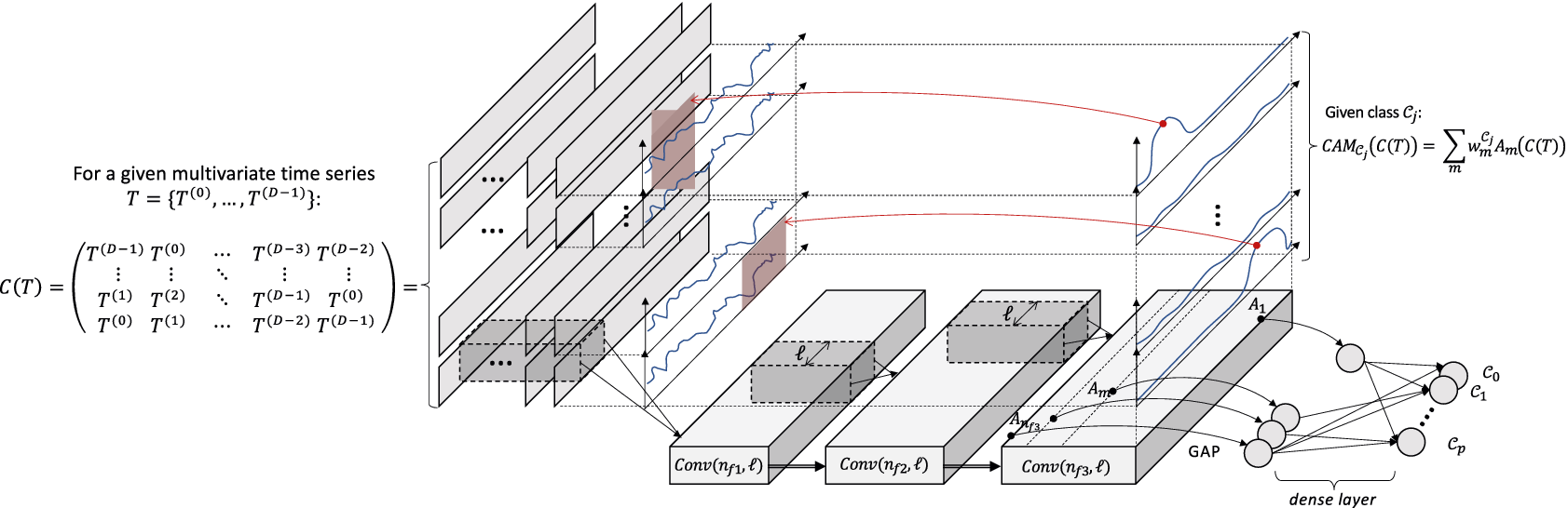
Observe that multiple permutations of the original multivariate series (provided only by the different rows of $ C(T) $
) will be processed by several convolutional filters, enabling the kernel to examine multiple different combinations of dimensions and subsequences. Note that the kernels of the dCNN will be sparse, which has a significant impact on overfitting.
$ C(T) $
) will be processed by several convolutional filters, enabling the kernel to examine multiple different combinations of dimensions and subsequences. Note that the kernels of the dCNN will be sparse, which has a significant impact on overfitting.
3.3. Variant architectures: dResNet and dInceptionTime
As mentioned earlier, any architecture using a GAP layer after the last convolutional layer can benefit from dCAM. Thus, different (and more sophisticated) architectures can be used with our approach. To that effect, we propose two new architectures dResNet and dInceptionTime, based on the state-of-the-art architectures ResNet (Wang et al., Reference Wang, Yan and Oates2017) and InceptionTime (Ismail Fawaz et al., Reference Ismail Fawaz, Lucas, Forestier, Pelletier, Schmidt, Weber, Webb, Idoumghar, Muller and Petitjean2020). The transformations that lead to dResNet and dInceptionTime are very similar to that from CNN to dCNN, using $ C(T) $
as input to the transformed networks. The convolutional layers are transformed from 1D (as proposed in the original architecture (Wang et al., Reference Wang, Yan and Oates2017; Ismail Fawaz et al., Reference Ismail Fawaz, Lucas, Forestier, Pelletier, Schmidt, Weber, Webb, Idoumghar, Muller and Petitjean2020)) to 2D. Similarly to dCNN, the kernel sizes are
$ C(T) $
as input to the transformed networks. The convolutional layers are transformed from 1D (as proposed in the original architecture (Wang et al., Reference Wang, Yan and Oates2017; Ismail Fawaz et al., Reference Ismail Fawaz, Lucas, Forestier, Pelletier, Schmidt, Weber, Webb, Idoumghar, Muller and Petitjean2020)) to 2D. Similarly to dCNN, the kernel sizes are $ \left(D,\mathrm{\ell},1\right) $
and convolute over each row of
$ \left(D,\mathrm{\ell},1\right) $
and convolute over each row of $ C(T) $
independently.
$ C(T) $
independently.
We demonstrate in the experimental section that these architectures do not affect the usage of our proposed approach dCAM, and we evaluate the choice of architecture on both classification and discriminant feature identification. In the following sections, we describe our methods assuming the dCNN architecture. Nevertheless, it works exactly the same for the other two architectures.
3.4. Dimension-wise class activation map
At this point, we have our network trained to classify instances among classes $ {\mathcal{C}}_0,{\mathcal{C}}_1,\dots, {\mathcal{C}}_p $
. We now describe in detail how to compute dCAM that will identify discriminant features within dimensions. We assume that the network has to be accurate enough in order to provide a meaningful dCAM. At first glance, one can compute the regular Class Activation Map
$ {\mathcal{C}}_0,{\mathcal{C}}_1,\dots, {\mathcal{C}}_p $
. We now describe in detail how to compute dCAM that will identify discriminant features within dimensions. We assume that the network has to be accurate enough in order to provide a meaningful dCAM. At first glance, one can compute the regular Class Activation Map $ {\mathrm{CAM}}_{{\mathcal{C}}_j}\left(C(T)\right)={\sum}_m{w}_m^{{\mathcal{C}}_j}{A}_m\left(C(T)\right) $
. However, a high value on the
$ {\mathrm{CAM}}_{{\mathcal{C}}_j}\left(C(T)\right)={\sum}_m{w}_m^{{\mathcal{C}}_j}{A}_m\left(C(T)\right) $
. However, a high value on the $ {i}^{th} $
row at position
$ {i}^{th} $
row at position $ t $
on
$ t $
on $ {\mathrm{CAM}}_{{\mathcal{C}}_j}\left(C(T)\right) $
does not mean that the subsequence at position
$ {\mathrm{CAM}}_{{\mathcal{C}}_j}\left(C(T)\right) $
does not mean that the subsequence at position $ t $
on the
$ t $
on the $ {i}^{th} $
dimension is important for the classification. It instead means that the combination of dimensions at the
$ {i}^{th} $
dimension is important for the classification. It instead means that the combination of dimensions at the $ {i}^{th} $
row of
$ {i}^{th} $
row of $ C(T) $
is important.
$ C(T) $
is important.
3.4.1. Random permutation computations
Given those different combinations of dimensions (i.e., one row of $ C(T) $
) produce different outputs (i.e., the same row in
$ C(T) $
) produce different outputs (i.e., the same row in $ {\mathrm{CAM}}_{{\mathcal{C}}_j}\left(C(T)\right) $
), the positions of the dimensions within the
$ {\mathrm{CAM}}_{{\mathcal{C}}_j}\left(C(T)\right) $
), the positions of the dimensions within the $ C(T) $
rows have an impact on the Class Activation Map. Consequently, for a given combination of dimensions, we can assume that at least one dimension at a given position is responsible for the high value in the Class Activation Map row. For the remainder of this article, we use
$ C(T) $
rows have an impact on the Class Activation Map. Consequently, for a given combination of dimensions, we can assume that at least one dimension at a given position is responsible for the high value in the Class Activation Map row. For the remainder of this article, we use $ {\Sigma}_T $
as the set of all possible permutations of
$ {\Sigma}_T $
as the set of all possible permutations of $ T $
dimensions, and
$ T $
dimensions, and $ {S}_T^i\in {\Sigma}_T $
for a single permutation of
$ {S}_T^i\in {\Sigma}_T $
for a single permutation of $ T $
. For example, for a given data series
$ T $
. For example, for a given data series $ T=\left\{{T}^{(0)},{T}^{(1)},{T}^{(2)}\right\} $
, one possible permutation is
$ T=\left\{{T}^{(0)},{T}^{(1)},{T}^{(2)}\right\} $
, one possible permutation is $ {S}_T^i=\left\{{T}^{(1)},{T}^{(0)},{T}^{(2)}\right\} $
.
$ {S}_T^i=\left\{{T}^{(1)},{T}^{(0)},{T}^{(2)}\right\} $
.
Figure 3 depicts an example of Class Activation Maps for different permutations. In this figure, for three given permutations of $ T $
(i.e.,
$ T $
(i.e., $ {S}_T^0 $
,
$ {S}_T^0 $
, $ {S}_T^1 $
, and
$ {S}_T^1 $
, and $ {S}_T^2 $
), we notice that when
$ {S}_T^2 $
), we notice that when $ {T}^{(2)} $
is in position two of the second row of
$ {T}^{(2)} $
is in position two of the second row of $ C\left({S}_T^i\right) $
, the Class Activation Map
$ C\left({S}_T^i\right) $
, the Class Activation Map $ \mathrm{CAM}\left(C\left({S}_T^i\right)\right) $
is greater than when
$ \mathrm{CAM}\left(C\left({S}_T^i\right)\right) $
is greater than when $ {T}^{(2)} $
is not in position two. We infer that the second dimension of
$ {T}^{(2)} $
is not in position two. We infer that the second dimension of $ T $
in position two is responsible for the high value. Thus, we may examine different dimension combinations by keeping track of which dimension at which position is activating the Class Activation Map the most. In the remainder of this section, we describe the steps necessary to retrieve this information.
$ T $
in position two is responsible for the high value. Thus, we may examine different dimension combinations by keeping track of which dimension at which position is activating the Class Activation Map the most. In the remainder of this section, we describe the steps necessary to retrieve this information.
Definition 1. For a given data series $ T=\left\{{T}^{(0)},{T}^{(1)},\dots, {T}^{\left(D-1\right)}\right\} $
of length
$ T=\left\{{T}^{(0)},{T}^{(1)},\dots, {T}^{\left(D-1\right)}\right\} $
of length $ n $
and its input data structure
$ n $
and its input data structure $ C(T) $
, we define function
$ C(T) $
, we define function $ \mathrm{idx} $
, such that
$ \mathrm{idx} $
, such that $ \mathrm{idx}\left({T}^{(i)},{p}_j\right) $
returns the row indices in
$ \mathrm{idx}\left({T}^{(i)},{p}_j\right) $
returns the row indices in $ C(T) $
that contain the dimension
$ C(T) $
that contain the dimension $ {T}^{(i)} $
at position
$ {T}^{(i)} $
at position $ {p}_j $
.
$ {p}_j $
.
Example of Class Activation Map results for different permutations.

We can now define the following transformation $ \mathcal{M} $
.
$ \mathcal{M} $
.
Definition 2. For a given data series $ T=\left\{{T}^{(0)},{T}^{(1)},\dots, {T}^{\left(D-1\right)}\right\} $
of length
$ T=\left\{{T}^{(0)},{T}^{(1)},\dots, {T}^{\left(D-1\right)}\right\} $
of length $ n $
, a given class
$ n $
, a given class $ {\mathcal{C}}_j $
and Class Activation Map, we define
$ {\mathcal{C}}_j $
and Class Activation Map, we define $ \mathcal{M}\left({\mathrm{CAM}}_{{\mathcal{C}}_j}\left(C(T)\right)\right)\in {\mathrm{\mathbb{R}}}^{\left(D,D,n\right)} $
(with
$ \mathcal{M}\left({\mathrm{CAM}}_{{\mathcal{C}}_j}\left(C(T)\right)\right)\in {\mathrm{\mathbb{R}}}^{\left(D,D,n\right)} $
(with $ {\mathrm{CAM}}_{{\mathcal{C}}_j}\left(C(T)\right)\in {\mathrm{\mathbb{R}}}^{\left(D,n\right)} $
and
$ {\mathrm{CAM}}_{{\mathcal{C}}_j}\left(C(T)\right)\in {\mathrm{\mathbb{R}}}^{\left(D,n\right)} $
and $ {\mathrm{CAM}}_{{\mathcal{C}}_j}{\left(C(T)\right)}_i $
its
$ {\mathrm{CAM}}_{{\mathcal{C}}_j}{\left(C(T)\right)}_i $
its $ {i}^{th} $
row) as follows:
$ {i}^{th} $
row) as follows:
 $$ \mathcal{M}\left({\mathrm{CAM}}_{{\mathcal{C}}_j}\left(C(T)\right)\right)=\left(\begin{array}{ccc}{\mathrm{CAM}}_{{\mathcal{C}}_j}{\left(C(T)\right)}_{\mathrm{idx}\left({T}^{(0)},0\right)}& \dots & {\mathrm{CAM}}_{{\mathcal{C}}_j}{\left(C(T)\right)}_{\mathrm{idx}\left({T}^{(0)},D-1\right)}\\ {}{\mathrm{CAM}}_{{\mathcal{C}}_j}{\left(C(T)\right)}_{\mathrm{idx}\left({T}^{(1)},0\right)}& \dots & {\mathrm{CAM}}_{{\mathcal{C}}_j}{\left(C(T)\right)}_{\mathrm{idx}\left({T}^{(1)},D-1\right)}\\ {}:& \dots & :\\ {}{\mathrm{CAM}}_{{\mathcal{C}}_j}{\left(C(T)\right)}_{\mathrm{idx}\left({T}^{\left(D-1\right)},0\right)}& \dots & {\mathrm{CAM}}_{{\mathcal{C}}_j}{\left(C(T)\right)}_{\mathrm{idx}\left({T}^{\left(D-1\right)},D-1\right)}\end{array}\right)\hskip-0.1em . $$
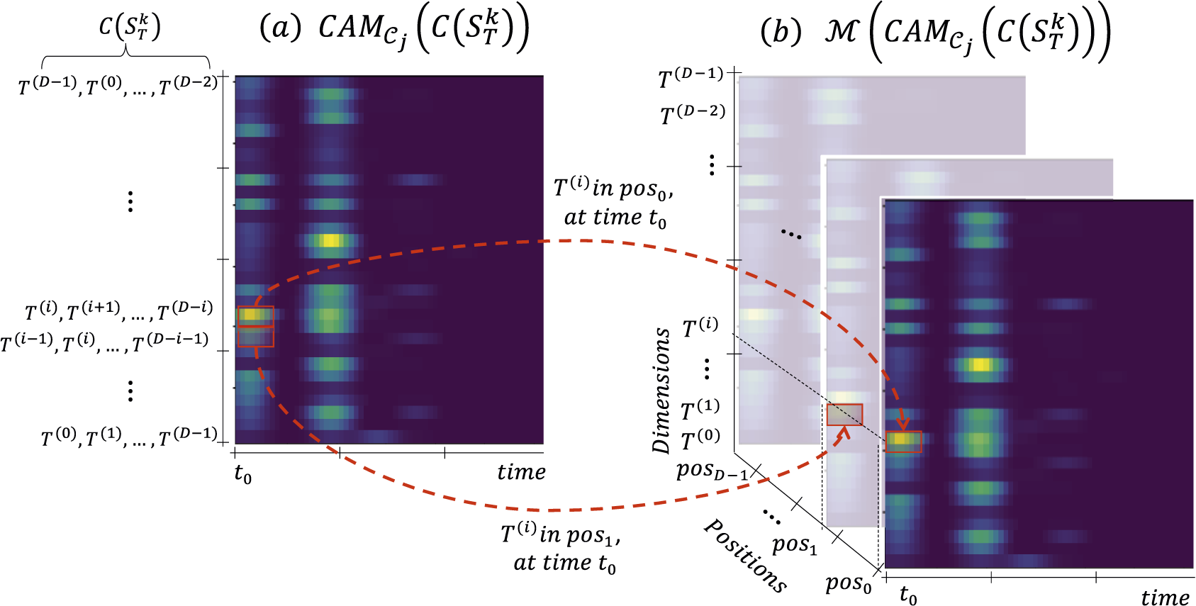
Figure 4 depicts the $ \mathcal{M} $
transformation. As explained in Definition 2, the
$ \mathcal{M} $
transformation. As explained in Definition 2, the $ \mathcal{M} $
transformation enriches the Class Activation Map by adding the dimension position information. Note that if we change the dimension order of
$ \mathcal{M} $
transformation enriches the Class Activation Map by adding the dimension position information. Note that if we change the dimension order of $ T $
, their
$ T $
, their $ \mathcal{M}\left({\mathrm{CAM}}_{{\mathcal{C}}_j}\left(C(T)\right)\right) $
changes as well. Indeed, for a given dimension
$ \mathcal{M}\left({\mathrm{CAM}}_{{\mathcal{C}}_j}\left(C(T)\right)\right) $
changes as well. Indeed, for a given dimension $ {T}^{(i)} $
and position
$ {T}^{(i)} $
and position $ {p}_j $
,
$ {p}_j $
, $ \mathrm{idx}\left({T}^{(i)},\hskip0.5em ,{p}_j\right) $
will not have the same value for two different dimension orders of
$ \mathrm{idx}\left({T}^{(i)},\hskip0.5em ,{p}_j\right) $
will not have the same value for two different dimension orders of $ T $
. Thus, computing
$ T $
. Thus, computing $ \mathcal{M}\left({\mathrm{CAM}}_{{\mathcal{C}}_j}\left(C(T)\right)\right) $
for different dimension orders of
$ \mathcal{M}\left({\mathrm{CAM}}_{{\mathcal{C}}_j}\left(C(T)\right)\right) $
for different dimension orders of $ T $
will provide distinct information regarding the importance of a given position (subsequence) in a given dimension. We expect that subsequences (of a specific dimension) that discriminate one class from another will also be associated (most of the time) with a high value in the Class Activation Map.
$ T $
will provide distinct information regarding the importance of a given position (subsequence) in a given dimension. We expect that subsequences (of a specific dimension) that discriminate one class from another will also be associated (most of the time) with a high value in the Class Activation Map.
Transformation $ \mathcal{M} $
for a given data series
$ \mathcal{M} $
for a given data series $ T $
.
$ T $
.
3.4.2. Merging permutations
We compute $ \mathcal{M}\left({\mathrm{CAM}}_{{\mathcal{C}}_j}\left(C\left({S}_T\right)\right)\right) $
for different
$ \mathcal{M}\left({\mathrm{CAM}}_{{\mathcal{C}}_j}\left(C\left({S}_T\right)\right)\right) $
for different $ {S}_T\in {\Sigma}_T $
. Note that the total number of permutations for high-dimensional data series
$ {S}_T\in {\Sigma}_T $
. Note that the total number of permutations for high-dimensional data series $ \mid {\Sigma}_T\mid $
is enormous. In practice, we only compute
$ \mid {\Sigma}_T\mid $
is enormous. In practice, we only compute $ \mathcal{M} $
for a randomly selected subset of
$ \mathcal{M} $
for a randomly selected subset of $ {\Sigma}_T $
. We thus merge
$ {\Sigma}_T $
. We thus merge $ k=\mid {\Sigma}_T\mid $
permutations
$ k=\mid {\Sigma}_T\mid $
permutations $ {S}_T^k $
, by computing the averaged matrix
$ {S}_T^k $
, by computing the averaged matrix $ {\overline{\mathcal{M}}}_{{\mathcal{C}}_j}(T) $
of all the
$ {\overline{\mathcal{M}}}_{{\mathcal{C}}_j}(T) $
of all the $ \mathcal{M} $
transformations of the permutations. Formally,
$ \mathcal{M} $
transformations of the permutations. Formally, $ {\overline{\mathcal{M}}}_{{\mathcal{C}}_j}(T) $
is defined as follows:
$ {\overline{\mathcal{M}}}_{{\mathcal{C}}_j}(T) $
is defined as follows:
 $$ {\overline{\mathcal{M}}}_{{\mathcal{C}}_j}(T)=\frac{1}{\mid {\Sigma}_T\mid}\sum \limits_{S_T^k\in {\Sigma}_T}\mathcal{M}\left({\mathrm{CAM}}_{{\mathcal{C}}_j}\left(C\left({S}_T^k\right)\right)\right) $$
Figure 5 illustrates the process of computing $ {\overline{\mathcal{M}}}_{{\mathcal{C}}_j}(T) $
from the set of permutations of
$ {\overline{\mathcal{M}}}_{{\mathcal{C}}_j}(T) $
from the set of permutations of $ T $
,
$ T $
, $ {\Sigma}_T $
.
$ {\Sigma}_T $
. $ {\overline{\mathcal{M}}}_{{\mathcal{C}}_j}(T) $
can be seen as a summarization of the importance of each dimension at each position in
$ {\overline{\mathcal{M}}}_{{\mathcal{C}}_j}(T) $
can be seen as a summarization of the importance of each dimension at each position in $ C(T) $
, for all the computed permutations. Figure 5b’ (at the top of the figure) depicts
$ C(T) $
, for all the computed permutations. Figure 5b’ (at the top of the figure) depicts $ {\overline{\mathcal{M}}}_{{\mathcal{C}}_j}{(T)}_d $
, which corresponds to the
$ {\overline{\mathcal{M}}}_{{\mathcal{C}}_j}{(T)}_d $
, which corresponds to the $ {d}^{th} $
row (i.e., the dotted box in Figure 5b) of
$ {d}^{th} $
row (i.e., the dotted box in Figure 5b) of $ {\overline{\mathcal{M}}}_{{\mathcal{C}}_j}(T) $
. Each row of
$ {\overline{\mathcal{M}}}_{{\mathcal{C}}_j}(T) $
. Each row of $ {\overline{\mathcal{M}}}_{{\mathcal{C}}_j}{(T)}_d $
corresponds to the average activation of dimension
$ {\overline{\mathcal{M}}}_{{\mathcal{C}}_j}{(T)}_d $
corresponds to the average activation of dimension $ d $
(for each timestamp) when dimension
$ d $
(for each timestamp) when dimension $ d $
is in a given position in
$ d $
is in a given position in $ C(T) $
.
$ C(T) $
.
dCAM computation framework.

Note that all permutations of $ T $
are forwarded into the dCNN network without training it again. Thus, even though the permutations of
$ T $
are forwarded into the dCNN network without training it again. Thus, even though the permutations of $ T $
generate radically different inputs to the network, the network can still classify most of the instances correctly. For
$ T $
generate radically different inputs to the network, the network can still classify most of the instances correctly. For $ k $
permutations, we use
$ k $
permutations, we use $ {n}_g $
to denote the number of permutations the model has correctly classified.
$ {n}_g $
to denote the number of permutations the model has correctly classified.
3.4.3. dCAM extraction
We can now use the previously computed $ {\overline{\mathcal{M}}}_{{\mathcal{C}}_j} $
to extract explanatory information on which subsequences are considered important by the network. First, we note that each row of
$ {\overline{\mathcal{M}}}_{{\mathcal{C}}_j} $
to extract explanatory information on which subsequences are considered important by the network. First, we note that each row of $ C(T) $
corresponds to the input format of the standard CNN architecture. Thus, we expect that the result of a row of
$ C(T) $
corresponds to the input format of the standard CNN architecture. Thus, we expect that the result of a row of $ {\overline{\mathcal{M}}}_{{\mathcal{C}}_j} $
(1 of the 10 lines in Figure 5b) is similar to the standard CAM. Hence, we can assume that
$ {\overline{\mathcal{M}}}_{{\mathcal{C}}_j} $
(1 of the 10 lines in Figure 5b) is similar to the standard CAM. Hence, we can assume that  is equivalent to standard Class Activation Map $ {\mathrm{CAM}}_{{\mathcal{C}}_j}(T) $
(this approximation is depicted in Figure 5d). Moreover, we can extract temporal information per dimension in addition to the global temporal information. We know that for a given position
$ {\mathrm{CAM}}_{{\mathcal{C}}_j}(T) $
(this approximation is depicted in Figure 5d). Moreover, we can extract temporal information per dimension in addition to the global temporal information. We know that for a given position $ p $
and a given dimension
$ p $
and a given dimension $ d $
,
$ d $
, $ {\overline{\mathcal{M}}}_{{\mathcal{C}}_j}^{d,p}(T) $
represents the averaged activation for a given set of permutations. If the activation
$ {\overline{\mathcal{M}}}_{{\mathcal{C}}_j}^{d,p}(T) $
represents the averaged activation for a given set of permutations. If the activation $ {\overline{\mathcal{M}}}_{{\mathcal{C}}_j}^{d,p}(T) $
for a given dimension is constant (regardless of its value or the position
$ {\overline{\mathcal{M}}}_{{\mathcal{C}}_j}^{d,p}(T) $
for a given dimension is constant (regardless of its value or the position $ p $
), then the position of dimension
$ p $
), then the position of dimension $ d $
is not important, and no subsequence in that dimension
$ d $
is not important, and no subsequence in that dimension $ d $
is discriminant. On the other hand, a high or low value at a specific position
$ d $
is discriminant. On the other hand, a high or low value at a specific position $ p $
means that the subsequence at this specific position is discriminant. While it is intuitive to interpret a high value, interpreting a low value is counterintuitive. Usually, a subsequence at position
$ p $
means that the subsequence at this specific position is discriminant. While it is intuitive to interpret a high value, interpreting a low value is counterintuitive. Usually, a subsequence at position $ p $
with a low value should be regarded as nondiscriminant. Nevertheless, if the activation is low for
$ p $
with a low value should be regarded as nondiscriminant. Nevertheless, if the activation is low for $ p $
and high for other positions, then the subsequence at position
$ p $
and high for other positions, then the subsequence at position $ p $
is the consequence of the low value and is thus discriminant. We experimentally observe this situation, where a nondiscriminant dimension has a constant activation per position (e.g., see dotted red rectangle in Figure 5b: this pattern corresponds to a nondiscriminant subsequence of the dataset). On the contrary, for discriminant dimensions, we observe a strong variance for the activation per position: either high values or low values (e.g., see solid red rectangles in Figure 5b: these patterns correspond to the (injected) discriminant subsequences highlighted in red in Figure 5e). We thus can extract the significant subsequences per dimension by computing the variance of all positions of a given dimension. We can filter out the irrelevant temporal windows using the averaged
$ p $
is the consequence of the low value and is thus discriminant. We experimentally observe this situation, where a nondiscriminant dimension has a constant activation per position (e.g., see dotted red rectangle in Figure 5b: this pattern corresponds to a nondiscriminant subsequence of the dataset). On the contrary, for discriminant dimensions, we observe a strong variance for the activation per position: either high values or low values (e.g., see solid red rectangles in Figure 5b: these patterns correspond to the (injected) discriminant subsequences highlighted in red in Figure 5e). We thus can extract the significant subsequences per dimension by computing the variance of all positions of a given dimension. We can filter out the irrelevant temporal windows using the averaged $ \mu \left({\overline{\mathcal{M}}}_{{\mathcal{C}}_j}(T)\right) $
for all dimensions, and use the variance to identify the important dimensions in the relevant temporal windows. Formally, we define
$ \mu \left({\overline{\mathcal{M}}}_{{\mathcal{C}}_j}(T)\right) $
for all dimensions, and use the variance to identify the important dimensions in the relevant temporal windows. Formally, we define $ {\mathrm{dCAM}}_{{\mathcal{C}}_j}(T) $
as follows.
$ {\mathrm{dCAM}}_{{\mathcal{C}}_j}(T) $
as follows.
Definition 3. For a given data series $ T $
and a given class
$ T $
and a given class $ {\mathcal{C}}_i $
,
$ {\mathcal{C}}_i $
, $ {\mathrm{dCAM}}_{{\mathcal{C}}_j}(T) $
is defined as:
$ {\mathrm{dCAM}}_{{\mathcal{C}}_j}(T) $
is defined as:

3.5. Time complexity analysis
3.5.1. Training step
CNN/ResNet/InceptionTime require $ O\left(\mathrm{\ell}\ast |T|\ast D\right) $
computations per kernel, while dCNN/dResNet/dInceptionTime require
$ O\left(\mathrm{\ell}\ast |T|\ast D\right) $
computations per kernel, while dCNN/dResNet/dInceptionTime require $ O\left(\mathrm{\ell}\ast |T|\ast {D}^2\right) $
computations per kernel. Thus, the training time per epoch is higher for dCNN than CNN. However, given that the size of the input of dCNN is larger (containing
$ O\left(\mathrm{\ell}\ast |T|\ast {D}^2\right) $
computations per kernel. Thus, the training time per epoch is higher for dCNN than CNN. However, given that the size of the input of dCNN is larger (containing $ D $
permutations of a single series) than CNN, the number of epochs to reach convergence is lower for dCNN when compared to CNN. Intuitively, dCNN trains on more data during a single epoch. This leads to similar overall training times.
$ D $
permutations of a single series) than CNN, the number of epochs to reach convergence is lower for dCNN when compared to CNN. Intuitively, dCNN trains on more data during a single epoch. This leads to similar overall training times.
3.5.2. dCAM step
The CAM computation complexity is $ O\left(|T|\hskip0.3em \ast \hskip0.3em D\hskip0.3em \ast \hskip0.3em {n}_f\right) $
, where
$ O\left(|T|\hskip0.3em \ast \hskip0.3em D\hskip0.3em \ast \hskip0.3em {n}_f\right) $
, where $ {n}_f $
is the number of filters in the last convolutional layer. Let
$ {n}_f $
is the number of filters in the last convolutional layer. Let $ {N}_f=\left[{n}_{f_1},\dots {n}_{f_n}\right] $
be the number of filters of the
$ {N}_f=\left[{n}_{f_1},\dots {n}_{f_n}\right] $
be the number of filters of the $ n $
convolutional layers. Then, a forward pass has time complexity
$ n $
convolutional layers. Then, a forward pass has time complexity $ O\left(\mathrm{\ell}\ast |T|\ast {D}^2\ast {\sum}_{n_{f_i}\in {N}_f}{n}_{f_i}\right) $
. In dCAM, we evaluate
$ O\left(\mathrm{\ell}\ast |T|\ast {D}^2\ast {\sum}_{n_{f_i}\in {N}_f}{n}_{f_i}\right) $
. In dCAM, we evaluate $ k $
different permutations. Thus, the overall dCAM complexity is
$ k $
different permutations. Thus, the overall dCAM complexity is $ O\left(k\hskip0.3em \ast \hskip0.5em \mathrm{\ell}\hskip0.5em \ast \hskip0.3em |T|\hskip0.5em \ast \hskip0.5em {D}^2\ast \hskip0.3em {\sum}_{n_{f_i}\in {N}_f}{n}_{f_i}\right) $
. Observe that since the
$ O\left(k\hskip0.3em \ast \hskip0.5em \mathrm{\ell}\hskip0.5em \ast \hskip0.3em |T|\hskip0.5em \ast \hskip0.5em {D}^2\ast \hskip0.3em {\sum}_{n_{f_i}\in {N}_f}{n}_{f_i}\right) $
. Observe that since the $ k $
permutations can be computed in parallel, the most important parameter for the execution time is
$ k $
permutations can be computed in parallel, the most important parameter for the execution time is $ D $
.
$ D $
.
3.6. Further observations
3.6.1. Permutations success as a proxy
As previously explained, we assume that dCAM is meaningful if and only if the deep neural network classification is accurate. We also assume that classification accuracy impacts the number of correctly classified permutations. As in real use cases, labels may not be available, and both classification and discriminant feature identification accuracy may not be computed. Therefore, the number of correctly classified permutations (called $ {n}_g $
) could be used as a proxy to assess the quality of the explanation. More precisely, a low value of
$ {n}_g $
) could be used as a proxy to assess the quality of the explanation. More precisely, a low value of $ {n}_g $
indicates that the model is not efficient in classifying a time series regardless of the permutation. On the contrary, a high value of
$ {n}_g $
indicates that the model is not efficient in classifying a time series regardless of the permutation. On the contrary, a high value of $ {n}_g $
indicates that, whatever the permutations of the time series dimensions, the model is able to classify correctly the time series. Therefore, as dCAM uses different permutations to find back which dimensions correspond to discriminant features, a low value of
$ {n}_g $
indicates that, whatever the permutations of the time series dimensions, the model is able to classify correctly the time series. Therefore, as dCAM uses different permutations to find back which dimensions correspond to discriminant features, a low value of $ {n}_g $
indicates that the discriminant features identified by dCAM might not be meaningful.
$ {n}_g $
indicates that the discriminant features identified by dCAM might not be meaningful.
3.6.2. From local to global explanations
We have so far assumed that dCAM is applied to a single multivariate data series and provides corresponding explanations. In the case where we need to analyze a set of series though, we can use dCAM on each one independently and then aggregate the dCAM results in order to identify global discriminant features. (The problem of local and global explanations has been discussed in other studies as well (Jacob et al., Reference Jacob, Song, Stiegler, Rad, Diao and Tatbul2021)). Section 5 provides an example of how to get a global explanation of a specific use case. In future work, we will study other possibilities to merge dCAMs of instances of the same class.
3.6.3. Limitations: the dimension order problem
Even though this method is able to detect important subsequences within a multivariate data series, the use of dimension permutations can be problematic for specific time series. Such architecture is based on the use of dimension permutations as a fundamental principle. Thus, if the discriminant factor between two classes remains on the positions of the dimensions (e.g., having the same multivariate data series but with dimensions at different positions between two instances of two classes), one cannot use our proposed approach. Such a scenario is plausible for multivariate time series measured from a graph of sensors where the position of each sensor with regards to the other matters. In such cases, the differences between two events (i.e., two classes) might be explained by the geographical position of a specific pattern, resulting in discriminant features based on the order of the dimensions.
3.6.4. Limitations: large number of dimensions
Our proposed approach uses a new data structure $ C(T) $
. However,
$ C(T) $
. However, $ C(T) $
has a memory complexity of
$ C(T) $
has a memory complexity of $ O\left({D}^2\right) $
. Such memory complexity can be problematic for specific time series with many dimensions. Such large time series would imply reducing the batch size during the training phase such that an entire batch fits the memory of a CPU or GPU. As many data points in
$ O\left({D}^2\right) $
. Such memory complexity can be problematic for specific time series with many dimensions. Such large time series would imply reducing the batch size during the training phase such that an entire batch fits the memory of a CPU or GPU. As many data points in $ C(T) $
are redundant, an interesting research direction is to optimize the memory complexity to
$ C(T) $
are redundant, an interesting research direction is to optimize the memory complexity to $ O(D) $
.
$ O(D) $
.
3.6.5. Limitations: CAM-related constraints
As mentioned in Section 2.2, the Class Activation Map can only be used if (1) a Global Average Pooling layer has been used before the softmax classifier and (2) the model accuracy is high enough. Consequently, only the standard architectures CNN and ResNet proposed in the literature, combined with a global average pooling layer, can benefit from CAM. Therefore, other layers or combinations of the convolutional layers outputs (such as flattening operations) limit the application and the usage of CAM. As dCAM is based on CAM, the above constraints also hold for dCAM.
4. Classification experimental evaluation
We now present the results of the experimental evaluation with several real datasets from different domains. Our code and datasets are available online (dCAM, 2022).
4.1. Experimental setup
We implemented our algorithms in Python 3.5 using PyTorch (Paszke et al., Reference Paszke, Gross, Massa, Lerer, Bradbury, Chanan, Killeen, Lin, Gimelshein, Antiga, Desmaison, Kopf, Yang, DeVito, Raison, Tejani, Chilamkurthy, Steiner, Fang, Bai and Chintala2019). The evaluation was conducted on a server with Intel Core i7-8750H CPU 2.20GHz * 12, with 31.3GB RAM, and Quadro P1000/PCle/SSE2 GPU with 4.2GB RAM.
4.1.1. Datasets
We conduct our experimental evaluation using real datasets injected with known discriminant patterns. We use the StarLightCurves (classes 2 and 3 only) and ShapesAll (classes 1 and 2 only) datasets from the UCR archive (Dau et al., Reference Dau, Bagnall, Kamgar, Yeh, Zhu, Gharghabi, Ratanamahatana and Keogh2019), in which we inject subsequences that will generate discriminant features. We build two types of datasets to study the ability of the algorithms to identify the discriminant patterns guiding the classification decision, (1) when these patterns occur in a subset of the dimensions at different timestamps, and (2) when these patterns occur in a subset of the dimensions at the same timestamp.
-
(1) For Type 1 datasets, we build each dimension of Class 1 by concatenating random instances from one class of one of our two UCR seed datasets. We build Class 2 by injecting in the series of the other class of our two UCR datasets a pattern in $ 2 $
random dimensions at a random position in the series.
$ 2 $
random dimensions at a random position in the series. -
(2) For Type 2 datasets, we build each dimension of Class 1 by concatenating random instances from one of the classes of our two UCR datasets and injecting patterns from the other class in
$ x $
random dimensions and at different positions. We build Class 2 by injecting patterns at the same positions of
$ 2 $
random dimensions.


Examples of Type 1 and Type 2 5-dimensional datasets based on StarLightCurves are depicted in Figure 6a,b, respectively. In our experiments, we generate 1000 time series for the Type 1 synthetic dataset and 1000 time series for the Type 2 synthetic dataset.
Synthetic datasets: (a) Type 1, in which the discriminant subsequence is two injected patterns from class 2 StarLightCurves dataset in random dimensions at random positions, (b) Type 2, in which the discriminant factor is the fact that the two injected patterns are injected at the same position.
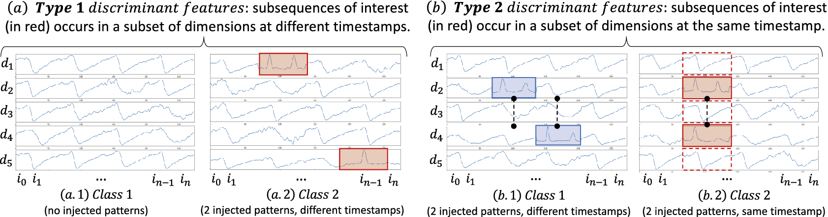
4.1.2. Evaluation measures
We first evaluate the classification accuracy, $ \mathrm{C} $
-
$ \mathrm{C} $
- $ \mathrm{acc} $
. This measure corresponds to the ratio of correctly classified instances among all instances in the test dataset. We then evaluate the discriminant features accuracy,
$ \mathrm{acc} $
. This measure corresponds to the ratio of correctly classified instances among all instances in the test dataset. We then evaluate the discriminant features accuracy, $ \mathrm{Dr} $
-
$ \mathrm{Dr} $
- $ \mathrm{acc} $
, for Class 1 (see Figure 6). We define
$ \mathrm{acc} $
, for Class 1 (see Figure 6). We define $ \mathrm{Dr} $
-
$ \mathrm{Dr} $
- $ \mathrm{acc} $
as the PR-AUC for CAM/cCAM/dCAM obtained from the models and the ground-truth. The ground-truth is a series that has
$ \mathrm{acc} $
as the PR-AUC for CAM/cCAM/dCAM obtained from the models and the ground-truth. The ground-truth is a series that has $ 1 $
at the positions of discriminant features (see Figure 6a.2): ground-truth contains
$ 1 $
at the positions of discriminant features (see Figure 6a.2): ground-truth contains $ 1 $
at the positions of the injected patterns, marked with the red rectangles, and
$ 1 $
at the positions of the injected patterns, marked with the red rectangles, and $ 0 $
otherwise). We motivate the choice of PR-AUC (instead of ROC-AUC) because we are more interested in measuring the accuracy of identifying the injected patterns (representing at max 0.02 percent of the dataset) than measuring the accuracy of not detecting the noninjected patterns. In this very unbalanced case, PR-AUC is more appropriate than ROC AUC (Davis and Goadrich, Reference Davis and Goadrich2006). Note that even though we annotate each point of the injected subsequences as discriminant, only some subparts of these sequences may be discriminant, thus leading to
$ 0 $
otherwise). We motivate the choice of PR-AUC (instead of ROC-AUC) because we are more interested in measuring the accuracy of identifying the injected patterns (representing at max 0.02 percent of the dataset) than measuring the accuracy of not detecting the noninjected patterns. In this very unbalanced case, PR-AUC is more appropriate than ROC AUC (Davis and Goadrich, Reference Davis and Goadrich2006). Note that even though we annotate each point of the injected subsequences as discriminant, only some subparts of these sequences may be discriminant, thus leading to $ \mathrm{Dr} $
-
$ \mathrm{Dr} $
- $ \mathrm{acc} $
less than
$ \mathrm{acc} $
less than $ 1 $
. Finally, for CNN/ResNet/InceptionTime we compute the
$ 1 $
. Finally, for CNN/ResNet/InceptionTime we compute the $ \mathrm{Dr} $
-
$ \mathrm{Dr} $
- $ \mathrm{acc} $
scores by assuming that their (univariate) CAM values are the same for all dimensions. We mark their
$ \mathrm{acc} $
scores by assuming that their (univariate) CAM values are the same for all dimensions. We mark their $ \mathrm{Dr} $
-
$ \mathrm{Dr} $
- $ \mathrm{acc} $
scores with a star in Table 1.
$ \mathrm{acc} $
scores with a star in Table 1. $ \mathrm{C} $
-
$ \mathrm{C} $
- $ \mathrm{acc} $
and
$ \mathrm{acc} $
and $ \mathrm{Dr} $
-
$ \mathrm{Dr} $
- $ \mathrm{acc} $
averaged accuracy for 10 runs for MTEX-CNN, ResNet, cResNet, dCNN, dResNet and dInceptionTime over synthetic datasets
$ \mathrm{acc} $
averaged accuracy for 10 runs for MTEX-CNN, ResNet, cResNet, dCNN, dResNet and dInceptionTime over synthetic datasets

4.1.3. Architectures and training
We compare our model, dCNN/dResNet/dInceptionTime, to the classical ResNet model (Wang et al., Reference Wang, Yan and Oates2017; Ismail Fawaz et al., Reference Ismail Fawaz, Forestier, Weber, Idoumghar and Muller2018; Fawaz et al., Reference Fawaz, Forestier, Weber, Idoumghar and Muller2019; Ismail Fawaz et al., Reference Ismail Fawaz, Lucas, Forestier, Pelletier, Schmidt, Weber, Webb, Idoumghar, Muller and Petitjean2020), and the cResNet baseline we introduced in Section 2. We only consider ResNet and cResNet architectures as we empirically observed that the latter are more accurate than CNN/cCNN and InceptionTime/cInceptionTime architectures. We are using the same architecture setup for all models. We then use CAM for ResNet, cCAM for cResNet, and dCAM for dCNN, dResNet, and dInceptionTime to identify discriminant features. For dCNN, we are using 5 convolutional layers with $ \left(\mathrm{64,128,256,256,256}\right) $
filters, respectively. We are using a kernel size of 3 and a padding of 2. For ResNet, cResNet and dResNet we use three blocks with three convolutional layers of 64 filters (for the first two blocks) and 128 layers (for the last block). We are using kernel sizes equal to 8, 5, and 3 for each block for the three layers of the block. For dInceptionTime, we use the same architecture as originally defined (Ismail Fawaz et al., Reference Ismail Fawaz, Lucas, Forestier, Pelletier, Schmidt, Weber, Webb, Idoumghar, Muller and Petitjean2020).
$ \left(\mathrm{64,128,256,256,256}\right) $
filters, respectively. We are using a kernel size of 3 and a padding of 2. For ResNet, cResNet and dResNet we use three blocks with three convolutional layers of 64 filters (for the first two blocks) and 128 layers (for the last block). We are using kernel sizes equal to 8, 5, and 3 for each block for the three layers of the block. For dInceptionTime, we use the same architecture as originally defined (Ismail Fawaz et al., Reference Ismail Fawaz, Lucas, Forestier, Pelletier, Schmidt, Weber, Webb, Idoumghar, Muller and Petitjean2020).
We also include MTEX-CNN (Assaf et al., Reference Assaf, Giurgiu, Bagehorn and Schumann2019)(MTEX) as a baseline, representative of other kinds of architectures that can provide a multivariate CAM. The explanation is computed separately for discriminant features and timestamps using grad-CAM (Selvaraju et al., Reference Selvaraju, Cogswell, Das, Vedantam, Parikh and Batra2017) (MTEX-grad). The latter is a variant of the usual CAM.
We split our dataset into training and validation sets with 80 and 20 percents of the total dataset, respectively (equally balanced between the two classes). The training dataset is used to train the model, and the validation dataset is used as a validation dataset during the training phase. We generate a fully new test dataset of 1000 time series (generated in the same manner as the initial 1000 time series used for the train and validation set) and evaluate $ \mathrm{C} $
-
$ \mathrm{C} $
- $ \mathrm{acc} $
and
$ \mathrm{acc} $
and $ \mathrm{Dr} $
-
$ \mathrm{Dr} $
- $ \mathrm{acc} $
. We train all models with a learning rate
$ \mathrm{acc} $
. We train all models with a learning rate $ \alpha =0.00001 $
, a maximum batch size of 16 instances (less if GPU memory cannot fit 16 instances), and a maximal number of epochs equal to 1000 (we use early stopping and stop before 1000 epochs if the model starts overfitting the test dataset). For dCAM, we use
$ \alpha =0.00001 $
, a maximum batch size of 16 instances (less if GPU memory cannot fit 16 instances), and a maximal number of epochs equal to 1000 (we use early stopping and stop before 1000 epochs if the model starts overfitting the test dataset). For dCAM, we use $ k=100 $
(number of random permutations), a value that we empirically verified (due to lack of space, a detailed analysis of the effect of
$ k=100 $
(number of random permutations), a value that we empirically verified (due to lack of space, a detailed analysis of the effect of $ k $
is in the full version of the article).
$ k $
is in the full version of the article).
4.2. Accuracy evaluation
We now evaluate the classification accuracy ( $ \mathrm{C} $
-
$ \mathrm{C} $
- $ \mathrm{acc} $
) and the discriminant feature identification accuracy (
$ \mathrm{acc} $
) and the discriminant feature identification accuracy ( $ \mathrm{Dr} $
-
$ \mathrm{Dr} $
- $ \mathrm{acc} $
) on synthetically built datasets. Table 1 depicts both
$ \mathrm{acc} $
) on synthetically built datasets. Table 1 depicts both $ \mathrm{C} $
-
$ \mathrm{C} $
- $ \mathrm{acc} $
and
$ \mathrm{acc} $
and $ \mathrm{Dr} $
-
$ \mathrm{Dr} $
- $ \mathrm{acc} $
on Type 1 and 2 datasets when varying the number of dimensions from 10 to 100.
$ \mathrm{acc} $
on Type 1 and 2 datasets when varying the number of dimensions from 10 to 100.
Overall, we observe that all methods have better performance (both $ \mathrm{C} $
-
$ \mathrm{C} $
- $ \mathrm{acc} $
and
$ \mathrm{acc} $
and $ \mathrm{Dr} $
-
$ \mathrm{Dr} $
- $ \mathrm{acc} $
) on Type 1 datasets than on Type 2 datasets. This was expected since discriminant features located in single dimensions are easier to find than discriminant features that depend on several dimensions.
$ \mathrm{acc} $
) on Type 1 datasets than on Type 2 datasets. This was expected since discriminant features located in single dimensions are easier to find than discriminant features that depend on several dimensions.
We then notice that for low dimensional ( $ D=10 $
) datasets, ResNet, dResNet, dCNN and dInceptionTime are performing nearly perfect
$ D=10 $
) datasets, ResNet, dResNet, dCNN and dInceptionTime are performing nearly perfect $ \mathrm{C}-\mathrm{acc} $
. Moreover, ResNet and MTEX-CNN are performing well for low-dimensional data series but start to fail for a more significant number of dimensions. While the drop is already significant for the Type 1 dataset built from the StarLightCurve dataset, it is even stronger for Type 2 datasets, for which ResNet fails to classify instances with a number of dimensions
$ \mathrm{C}-\mathrm{acc} $
. Moreover, ResNet and MTEX-CNN are performing well for low-dimensional data series but start to fail for a more significant number of dimensions. While the drop is already significant for the Type 1 dataset built from the StarLightCurve dataset, it is even stronger for Type 2 datasets, for which ResNet fails to classify instances with a number of dimensions $ D\ge 20 $
. On the contrary, dCNN, dResNet, and dInceptionTime, which use the random permutations in the input, are not sensitive to the number of dimensions and have an almost perfect
$ D\ge 20 $
. On the contrary, dCNN, dResNet, and dInceptionTime, which use the random permutations in the input, are not sensitive to the number of dimensions and have an almost perfect $ \mathrm{C} $
-
$ \mathrm{C} $
- $ \mathrm{acc} $
for most of Type 1 datasets. We observe a
$ \mathrm{acc} $
for most of Type 1 datasets. We observe a $ \mathrm{C} $
-
$ \mathrm{C} $
- $ \mathrm{acc} $
drop for dCNN, dResNet, and dInceptionTime as dimensions increase for Type 2 datasets. However, this drop is significantly less pronounced than that of ResNet. Overall, dCNN, dResNet, and dInceptionTime, which have on average the three highest ranks, are the most accurate methods.
$ \mathrm{acc} $
drop for dCNN, dResNet, and dInceptionTime as dimensions increase for Type 2 datasets. However, this drop is significantly less pronounced than that of ResNet. Overall, dCNN, dResNet, and dInceptionTime, which have on average the three highest ranks, are the most accurate methods.
Regarding cResNet, although it achieves a nearly perfect $ \mathrm{C}\hbox{-} \mathrm{acc} $
for Type 1 datasets, we observe that it fails to classify correctly instances of Type 2 datasets. As explained in Section 2, the input data structure is not rich enough to allow comparisons among dimensions, which is the main way to find discriminant features between the two classes of Type 2 datasets. We also observe that MTEX-CNN fails to classify instances of Type 2 datasets. Thus, this architecture is not correctly detecting the discriminant features across different dimensions. Overall, Figure 7a shows that dCNN, dResNet, and dInceptionTime are equivalent to cResNet for Type 1 (Figure 7a.1), outperforming all the baselines for Type 2 (Figure 7a.2), and in general are better than the baselines (ResNet and cResNet) for both types (Figure 7a.3) with
$ \mathrm{C}\hbox{-} \mathrm{acc} $
for Type 1 datasets, we observe that it fails to classify correctly instances of Type 2 datasets. As explained in Section 2, the input data structure is not rich enough to allow comparisons among dimensions, which is the main way to find discriminant features between the two classes of Type 2 datasets. We also observe that MTEX-CNN fails to classify instances of Type 2 datasets. Thus, this architecture is not correctly detecting the discriminant features across different dimensions. Overall, Figure 7a shows that dCNN, dResNet, and dInceptionTime are equivalent to cResNet for Type 1 (Figure 7a.1), outperforming all the baselines for Type 2 (Figure 7a.2), and in general are better than the baselines (ResNet and cResNet) for both types (Figure 7a.3) with  ).
).
Evaluation of the influence of the number of dimensions on our approaches and the baselines $ \mathrm{C} $
-
$ \mathrm{C} $
- $ \mathrm{acc} $
and
$ \mathrm{acc} $
and $ \mathrm{Dr} $
-
$ \mathrm{Dr} $
- $ \mathrm{acc} $
.
$ \mathrm{acc} $
.
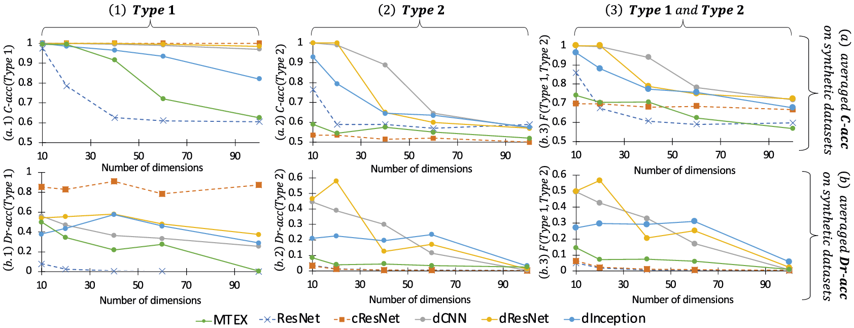
We now compare the different methods using the $ \mathrm{Dr} $
-
$ \mathrm{Dr} $
- $ \mathrm{acc} $
measure. We observe that the baseline cCAM (computed with cCNN) is outperforming CAM (computed with ResNet) and dCAM (with all of dCNN, dResNet, and dInceptionTime) for Type 1 datasets. This is explained by the fact that these classes can be discriminated by treating dimensions independently. Thus, cCAM (with no comparisons between dimensions) is naturally the best solution. Nevertheless, as Type 2 datasets require comparisons among dimensions to discriminate the classes, cCAM fails on them, with a
$ \mathrm{acc} $
measure. We observe that the baseline cCAM (computed with cCNN) is outperforming CAM (computed with ResNet) and dCAM (with all of dCNN, dResNet, and dInceptionTime) for Type 1 datasets. This is explained by the fact that these classes can be discriminated by treating dimensions independently. Thus, cCAM (with no comparisons between dimensions) is naturally the best solution. Nevertheless, as Type 2 datasets require comparisons among dimensions to discriminate the classes, cCAM fails on them, with a $ \mathrm{Dr} $
-
$ \mathrm{Dr} $
- $ \mathrm{acc} $
very similar to the one of a random classifier. This confirms that such a baseline cannot be considered as a general solution for multivariate data series classification. We also observe that
$ \mathrm{acc} $
very similar to the one of a random classifier. This confirms that such a baseline cannot be considered as a general solution for multivariate data series classification. We also observe that $ \mathrm{Dr} $
-
$ \mathrm{Dr} $
- $ \mathrm{acc} $
of the explanation method of MTEX-CNN (MTEX-grad) is lower than dCAM for Type 1 and close to
$ \mathrm{acc} $
of the explanation method of MTEX-CNN (MTEX-grad) is lower than dCAM for Type 1 and close to $ \mathrm{Dr} $
-
$ \mathrm{Dr} $
- $ \mathrm{acc} $
of cCAM for Type 2, meaning that it cannot identify discriminant features of Type 2 datasets.
$ \mathrm{acc} $
of cCAM for Type 2, meaning that it cannot identify discriminant features of Type 2 datasets.
We then compare CAM and dCAM (used with dCNN, dResNet, and dInceptionTime). We note that dCAM significantly outperforms CAM. As depicted in Figure 7b, we also observe that $ \mathrm{Dr} $
-
$ \mathrm{Dr} $
- $ \mathrm{acc} $
reduces for all models as the number of dimensions increases. Nevertheless,
$ \mathrm{acc} $
reduces for all models as the number of dimensions increases. Nevertheless, $ \mathrm{Dr} $
-
$ \mathrm{Dr} $
- $ \mathrm{acc} $
of dCAM remains relatively high for both Type 1 (Figure 7b.1)) and Type 2 (Figure 7b.2) datasets (for a number of dimensions under
$ \mathrm{acc} $
of dCAM remains relatively high for both Type 1 (Figure 7b.1)) and Type 2 (Figure 7b.2) datasets (for a number of dimensions under $ 60 $
).
$ 60 $
).
This result demonstrates the superiority of dCAM over state-of-the-art methods. The superiority of dCAM is also confirmed by looking at the average ranks in Table 1, which indicates that dCAM computed from dResNet has the highest rank of $ 2.15 $
.
$ 2.15 $
.
5. Use case: precursors of anomalous vibration detection in nuclear power plants
We now illustrate the applicability and interest of our method in a real-world application. This use case is about discovering possible precursors of unwanted vibration happening in turbine-driven feed-water pump systems inside French nuclear power plants. These pumps (two different pumps noted, TPA1 and TPA2) aim to increase the water pressure (from 1 to 80 bar) before passing the water through the steam generator (with a pressure of 80 bar). However, these vibrations are problematic when the pump’s position varies by a few microns, and a boolean sensor is activated when it happens. Thus, knowledge experts are interested in finding if there exist possible precursors of these unwanted vibrations in other sensors surrounding the pump and discovering unusual patterns that could explain why the pump is vibrating or at least alert the imminent occurrence of vibrations.
5.1. Dataset and use case description
At this point, we need to create our datasets of abnormal data series (i.e., vibrations) and anomaly-free data series. Following the suggestion of expert knowledge, we selected 120 sensors inside 12 subsystems of the nuclear power plants. Figure 8a summarizes the subsystems analyzed and the number of sensors collected. We collected every unwanted vibration that happened in every French 1300 MW nuclear plant. In total, we have 444 vibrations. We then create our multivariate data series by selecting every sensor’s measurement between 75 minutes before the vibrations and 5 minutes after. We set the acquisition rate to 1 point every 6 seconds. Each multivariate data series contains 96,000 points. Next, we note the set of data series containing a vibration $ {T}_{\mathcal{M}}^A $
. We then select 444 intervals of 80 minutes for which no vibration has been recorded at least one day before and after. Finally, we note the set of data series without any vibration
$ {T}_{\mathcal{M}}^A $
. We then select 444 intervals of 80 minutes for which no vibration has been recorded at least one day before and after. Finally, we note the set of data series without any vibration $ {T}_{\mathcal{M}}^N $
. We also selected the nonvibration periods to be under the same operating conditions as the vibration periods. Namely, when the nuclear facility ramps up or down between 15% and 67% of maximum power. This area, where the second feed-water pump is coupled, is conducive to vibrations. This is a critical step that must be conducted thoroughly. Otherwise, the precursors that would be highlighted would be the already-known difference in operational conditions and solicitations. In this specific case, we used the sensors related to the power regime: its distribution is the same across both classes. We also took the same distribution of years for both classes to minimize the influence of degradation due to aging. What we want to highlight are unexpected solicitations that would lead to vibrations later. This will trigger immediate and cost-effective corrective actions. We thus have in total 888 multivariate data series (for which 444 of them correspond to unwanted vibrations) of
$ {T}_{\mathcal{M}}^N $
. We also selected the nonvibration periods to be under the same operating conditions as the vibration periods. Namely, when the nuclear facility ramps up or down between 15% and 67% of maximum power. This area, where the second feed-water pump is coupled, is conducive to vibrations. This is a critical step that must be conducted thoroughly. Otherwise, the precursors that would be highlighted would be the already-known difference in operational conditions and solicitations. In this specific case, we used the sensors related to the power regime: its distribution is the same across both classes. We also took the same distribution of years for both classes to minimize the influence of degradation due to aging. What we want to highlight are unexpected solicitations that would lead to vibrations later. This will trigger immediate and cost-effective corrective actions. We thus have in total 888 multivariate data series (for which 444 of them correspond to unwanted vibrations) of $ D=120 $
dimensions. In total, the dataset contains 85,248,000 points. Formally, we define the dataset as
$ D=120 $
dimensions. In total, the dataset contains 85,248,000 points. Formally, we define the dataset as $ {T}_{\mathcal{M}}={T}_{\mathcal{M}}^N\cup {T}_{\mathcal{M}}^A $
, with
$ {T}_{\mathcal{M}}={T}_{\mathcal{M}}^N\cup {T}_{\mathcal{M}}^A $
, with $ {T}_{\mathcal{M}}^N,{T}_{\mathcal{M}}^A\in {\mathrm{\mathbb{R}}}^{\left(\mathrm{444,120,800}\right)} $
.
$ {T}_{\mathcal{M}}^N,{T}_{\mathcal{M}}^A\in {\mathrm{\mathbb{R}}}^{\left(\mathrm{444,120,800}\right)} $
.
Simplified scheme of the secondary circuit of 1300 MW nuclear power plant. We collect in total 120 sensors from 8 subsystems (solid black boxes) surrounding the feed-water pumps (TPA). Blue arrows: water flow. Red arrows: steam flows.

5.2. Experimental analysis
Overall, the task is to detect the vibration correctly and discover subsequences in one or several sensors that happened before the vibration and could potentially explain it. We tackle this task as defined in Problem 1 with dCNN/dCAM. Thus, we perform the following experiments. We first train dCNN to classify $ {T}_{\mathcal{M}}^A $
and
$ {T}_{\mathcal{M}}^A $
and $ {T}_{\mathcal{M}}^N $
. Formally, dCNN is defined as a function
$ {T}_{\mathcal{M}}^N $
. Formally, dCNN is defined as a function $ f:{T}_{\mathcal{M}}^{\mathcal{N}},{T}_{\mathcal{M}}^{\mathcal{A}}\to \left\{\mathcal{N},\mathcal{A}\right\} $
. We then use dCAM as a function
$ f:{T}_{\mathcal{M}}^{\mathcal{N}},{T}_{\mathcal{M}}^{\mathcal{A}}\to \left\{\mathcal{N},\mathcal{A}\right\} $
. We then use dCAM as a function $ g:{T}_{\mathcal{M}}^{\mathcal{A}},f\to S $
that returns the set
$ g:{T}_{\mathcal{M}}^{\mathcal{A}},f\to S $
that returns the set $ S $
of subsequences that explain the classification as the vibration class (as the red subsequences and rectangle depicted in Figure 8b,c). In practice, dCAM returns a multivariate data series score for each instance in
$ S $
of subsequences that explain the classification as the vibration class (as the red subsequences and rectangle depicted in Figure 8b,c). In practice, dCAM returns a multivariate data series score for each instance in $ {T}_{\mathcal{M}}^{\mathcal{A}} $
(as depicted in Figure 8b,c). In Section 4.2, we have shown that dResNet is slightly more accurate than dCNN and dInceptionTime. However, for simplicity, we used the most usual architecture dCNN as our baseline for this use case.
$ {T}_{\mathcal{M}}^{\mathcal{A}} $
(as depicted in Figure 8b,c). In Section 4.2, we have shown that dResNet is slightly more accurate than dCNN and dInceptionTime. However, for simplicity, we used the most usual architecture dCNN as our baseline for this use case.
5.2.1. Accuracy evaluation
We train the dCNN (we are using 5 convolutional layers with $ \left(\mathrm{64,128,256,256,256}\right) $
filters respectively; we are using a kernel size of 3 and a padding of 2) model on 70% of each class (
$ \left(\mathrm{64,128,256,256,256}\right) $
filters respectively; we are using a kernel size of 3 and a padding of 2) model on 70% of each class ( $ {T}_{\mathcal{M}}^N $
and
$ {T}_{\mathcal{M}}^N $
and $ {T}_{\mathcal{M}}^A $
) and we use the 30% left as a validation set. We set the batch size to 8 instances. We adopt an Early-stopping strategy to avoid overfitting. More precisely, we stop the training phase when the loss on the validation set is not reducing for the last 100 epochs. In total, we limit the training phase to 1000 epochs. It is important to note that the model and training parameters have been set empirically and based on the technical characteristics of our servers. More optimization with regards to the parameter selection could improve further the accuracy. However, the parameters listed above correspond to an adequate first baseline.
$ {T}_{\mathcal{M}}^A $
) and we use the 30% left as a validation set. We set the batch size to 8 instances. We adopt an Early-stopping strategy to avoid overfitting. More precisely, we stop the training phase when the loss on the validation set is not reducing for the last 100 epochs. In total, we limit the training phase to 1000 epochs. It is important to note that the model and training parameters have been set empirically and based on the technical characteristics of our servers. More optimization with regards to the parameter selection could improve further the accuracy. However, the parameters listed above correspond to an adequate first baseline.
Overall, over 10 random splits between training and validation sets, dCNN achieved at best 0.91 accuracy on the training set and 0.89 accuracy on the validation set. As the dCNN accuracy is high, we can now use dCAM to identify the discriminant subsequences (i.e., possible vibration precursors).
5.2.2. Quantitative evaluation
We then evaluate the relevance of the subsequences identified by our proposed approach dCAM. We first start by measuring the consistency of the detection (or activation) as regards the (1) temporality (i.e., are the subsequences detected close in time to the vibration?), (2) structural information (i.e., are the sensors closely related to the vibrating system?). As the experts are interested in discriminant features across the entire dataset, we perform the analysis listed above on the entire $ {T}_{\mathcal{M}}^{\mathcal{A}} $
(i.e., for time series included in the training and the validation set). As dCAM uses random permutations of the time series dimensions (resulting in inputs not used in the training set), the risks related to overfitting are limited and allow us to merge the training and validation set for this discriminant feature evaluation.
$ {T}_{\mathcal{M}}^{\mathcal{A}} $
(i.e., for time series included in the training and the validation set). As dCAM uses random permutations of the time series dimensions (resulting in inputs not used in the training set), the risks related to overfitting are limited and allow us to merge the training and validation set for this discriminant feature evaluation.
[Structural consistency] We then measure the average activation score per sensor for every timestamp. Figure 9 depicts the activation score box plot for each sensor using dCAM. We observe that the activation scores returned by dCAM vary significantly between different sensors. We can easily distinguish nine sensors out of 120 sensors. These sensors correspond to temperature measurements inside the feed-water pumps (sealing temperatures noted AGR605MT, AGR615MT for TPA1, and AGR606MT, AGR616MT for TPA2) and the outlet pump flow and pressures (noted APP011MD, APP061MP for TPA1, and APP012MD, APP062MP for TPA2). As highlighted in Figure 8a, AGR and APP are subsystems directly connected to the vibrating pump. Moreover, pressure and flow can directly influence the pump efficiency, with low-efficiency areas conducive to vibration events. Thus, the sensors highlighted by our proposed approach dCAM are very consistent with the knowledge from experts and the functional structure of the plant.
Aggregated activation score for dCAM per sensor for every timestamp. In red: are the names of the sensors that are overall highly activated and possibly contain one or several precursors.

[Temporal consistency] We first measure the evolution of the average activation score (for all sensors) in time obtained by dCAM (Figure 10a). Figure 10 depicts the quantile values for each timestamp. The solid red line is the median, while every dotted gray line corresponds to the 20%-quantiles. We first observe that the average activation score is higher when the vibration occurs (red vertical line in Figure 10). As it is unlikely to find precursors one hour before the vibration, we can thus confirm that dCAM results are consistent regarding temporality. We then observe the average anomaly score for some specific sensors (highlighted in red in Figure 9) that are the most activated across all vibration instances. We observe that, on average, all these sensors see their activation increases approximately 10 minutes before the vibrations. We thus explore in the following section the activated subsequences for these nine sensors.
Aggregated dCAM activation score for all sensors (a) and some specific sensors (b). Red shades correspond to quantile intervals (0.05–0.95,0.10–0.90,0.15–0.85, etc. for (a) and only 0.3–0.7, 0.4–0.6 for (b)). The solid red line is the median value for each timestamp.

5.2.3. Qualitative evaluation
We now analyze in detail the results returned by dCAM and discuss the information that the knowledge experts can gain from it. We mainly focus our analysis on the nine most activated sensors (i.e., sensors depicted in Figure 10(2)(b)). We cluster (computed with the usual k-mean using Euclidean distance) the 15 minutes long subsequences with the highest activation score for a vibration instance. The centroids of these clusters thus represent the different shape categories within each sensor detected by dCAM. Therefore we can limit our analysis to this reduced (but relevant) set of centroids. Figure 11(2) depicts the 15 minutes long subsequences clusters in the nine sensors mentioned above. For each cluster, the time distribution histogram is displayed below. We first notice that the majority of the subsequences (for all clusters) happened while the vibration is detected (such as, for instance, the cluster depicted in Figure 11(2)(b.2)). As understood by the experts, these subsequences correspond to a specific action (such as an increase or decrease of the water flow through the feed-water pump to either increase or decrease the power generated by the plant) that could lead to vibrations but that are not avoidable. Thus dCAM first permits the expert to confirm and visualize which subsequences are directly correlated to the vibration. Then, several subsequences detected by dCAM are anterior to the vibration (such as Figure 11(2)(a.2),(a.3),(b.1),(c.1),(c.2),(e.1),(g.3)). These subsequences could correspond to precursors of the vibration and would require to be carefully inspected by the experts. For instance, knowledge experts conclude that clusters such as in Figure 11(2)(e.1.1) correspond to unusual variations of the sealing temperature of the pump and lead them to investigate specific examples in detail. Overall, our proposed approach dCAM permits the experts to build a dictionary of patterns that can be related to a targeted anomaly. Thus the investigation by the expert could be significantly reduced.
(1) Cooccurrence graph connecting the activated subsequences clusters based on their cooccurrence in time. Subsequences clusters (*.*.1) (and their time distribution compared to the vibration timestamps (*.*.2)) detected as precursors of vibration by dCAM for the nine most activated sensors.
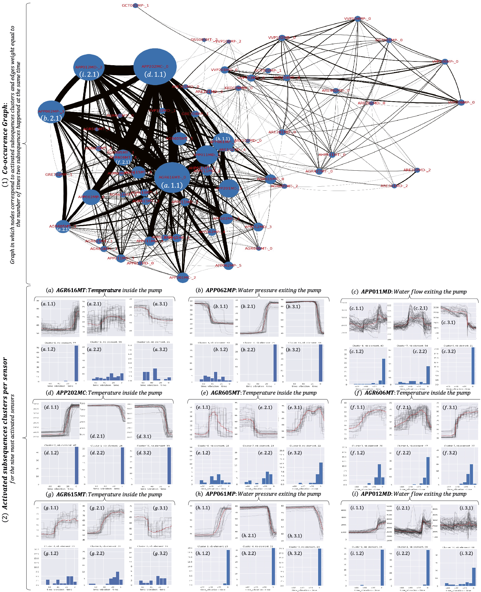
Finally, the patterns depicted in Figure 11(2) can be connected based on their cooccurrence in time. As a result, Figure 11(1) displays a graph in which nodes and edges are defined as follows: nodes correspond to activated subsequences clusters (with part of them illustrated in Figure 11(2)), edges weights (proportional to the line width) correspond to the number of times a subsequence of one cluster happened at the same time as a subsequence in another cluster. Thus, in Figure 11(1), we observe two distinct communities of sensors. The right community corresponds mainly to sensors from the ARE and VVP subsystems. On the other hand, the most significant community (i.e., on the left side of Figure 11(1)) are subsequences from the AGR and APP subsystems. These subsequences are mainly those illustrated in Figure 11(2). For instance, we learn from this graph that the patterns in Figure 11(2)(a.1.1), (d.1.1), (i.2.1), and (b.2.1) cooccurred very often before or during a vibration. Thus, such a graph can highlight more complex relationships between potential precursors.
6. Conclusions and future work
Even though data series classification using deep learning has attracted a lot of attention, existing techniques for explaining classification decisions fail in the case of multivariate data series. In this work, we describe a novel approach, dCAM, based on convolutional neural networks, which enables us to detect the discriminant subsequences within individual dimensions of a multivariate data series. The experimental evaluation with synthetic and real datasets demonstrates the benefits and superiority of our approach in discriminant feature discovery and classification explanation in multivariate time series. Our real use case applied to the nuclear power plants domain verifies the applicability and the interest of our solution. In future work, we plan to study in detail the effect that using permutations in the input has on the overall approach.
Author contribution
Conceptualization: P.B., M.M., E.R.; T.P., B.D.; Data curation: P.B., M.M., B.D.; Data visualization: P.B., M.M.; Methodology: P.B., B.D.; Writing—original draft: P.B.; M.M., E.R., T.P.
Competing interest
P.B. was employed at EDF R&D and received grants from EDF R&D. M.M. and E.R. are employed at EDF R&D. B.D. is employed at EDF. T.P. received grants from EDF R&D.
Data availability statement
The data and code supporting this study’s findings are openly available on GitHub. The code to reproduce the synthetic experiments can be found here: https://github.com/boniolp/dCAM. Restrictions apply to the availability of the data related to the industrial use case described in this article.
Funding statement
This work was supported by EDF R&D and ANRT French program.
Ethical standard
The research meets all ethical guidelines, including adherence to the legal requirements of the study country.


 Open access


Comments
No Comments have been published for this article.