





1 Introduction and Main Result
Let

and consider the nonlinear Schrödinger equation with a quasi-periodic potential on
$\mathbb Z^d$
 :
:

where
$\varepsilon $
 and
$\delta $
and
$\delta $
 are parameters in
$[0, 1]$
are parameters in
$[0, 1]$
 ,
$\boldsymbol {n}\in \mathbb Z^d$
,
$\boldsymbol {n}\in \mathbb Z^d$
 ,
$p\in \mathbb {N}$
,
$p\in \mathbb {N}$
 and
$\Delta (\boldsymbol {n}, \boldsymbol {n}')=\delta _{|\boldsymbol {n}-\boldsymbol {n}'|_1, 1}$
and
$\Delta (\boldsymbol {n}, \boldsymbol {n}')=\delta _{|\boldsymbol {n}-\boldsymbol {n}'|_1, 1}$
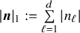
 denotes the adjacency Laplacian with
$|\boldsymbol {n}|_1:=\sum \limits _{\ell =1}^d|n_\ell |$
denotes the adjacency Laplacian with
$|\boldsymbol {n}|_1:=\sum \limits _{\ell =1}^d|n_\ell |$
 and
and

the potential V is a trigonometric polynomial:

with
$\Gamma _K\subset [-K, K]^d\setminus \{\boldsymbol {0}\},\ K\geq 1$
 and
and

where
$\#(\cdot )$
 denotes the cardinality of a set. We further assume that the set
$\Gamma _K$
denotes the cardinality of a set. We further assume that the set
$\Gamma _K$
 is maximal so that:

We assume that V is nondegenerate: For any fixed
$1\leq \ell \leq d$
 and
$(\theta _s)_{s\neq \ell }$
and
$(\theta _s)_{s\neq \ell }$
 ,
$f(\theta _\ell ):=V((\theta _s)_{s\neq \ell }, \theta _\ell )$
,
$f(\theta _\ell ):=V((\theta _s)_{s\neq \ell }, \theta _\ell )$
 is not a constant function in
$\theta _\ell .$
is not a constant function in
$\theta _\ell .$
 Note that the first condition in (1.2) then says that, in fact, each term in the polynomial is nondegenerate.
When
$\delta =0$
 , it is known from the breakthrough paper [Reference BourgainBou07] (cf. also the recent refinement [Reference Jitomirskaya, Liu and ShiJLS20]) that the linear operator

exhibits Anderson localization, namely pure point spectrum with exponentially decaying eigenfunctions, for small
$\varepsilon $
 , on a large set in
$(\boldsymbol {\alpha }, \boldsymbol {\theta })$
, on a large set in
$(\boldsymbol {\alpha }, \boldsymbol {\theta })$
 . It follows that when
$0<\varepsilon \ll 1$
. It follows that when
$0<\varepsilon \ll 1$
 , the linear Schrödinger equation

has only Anderson localized states, that is, roughly speaking, wave packets localized about the origin remain localized for all time.
The present paper addresses the persistence question when
$\delta \neq 0$
 , namely the existence of Anderson-localized-type solutions for the nonlinear Schrödinger equation (1.1) when
$0<\varepsilon , \delta \ll 1$
, namely the existence of Anderson-localized-type solutions for the nonlinear Schrödinger equation (1.1) when
$0<\varepsilon , \delta \ll 1$
 , under appropriate conditions on
$\boldsymbol {\alpha }$
, under appropriate conditions on
$\boldsymbol {\alpha }$
 and
$\boldsymbol {\theta }$
and
$\boldsymbol {\theta }$
 . Since both
$\varepsilon $
. Since both
$\varepsilon $
 and
$\delta $
and
$\delta $
 are small, we start from the (decoupled) equation

It has solutions of the form

where

and
$a_{\boldsymbol {n}}$
 decays rapidly. The solutions (1.6), in general, have infinite number of frequencies and are almost-periodic in time.
We study the persistence of the above type of solutions with finite (but arbitrary) number of frequencies in time, that is, the quasi-periodic in time solutions. Denoting the frequency by
$\boldsymbol {\omega }$
 ,
$\boldsymbol {\omega }= (\omega _1, \omega _2,\cdots , \omega _b)$
,
$\boldsymbol {\omega }= (\omega _1, \omega _2,\cdots , \omega _b)$
 , as an ansatz, we seek solutions to (1.1) in the form of a convergent series:

Note that solutions of the above form are consistent with the nonlinearity in (1.1).
Denote by
$\mathrm {meas}(\cdot )$
 the Lebesgue measure of a set. Let
$|\cdot |$
the Lebesgue measure of a set. Let
$|\cdot |$
 denote the supremum norm. We have
Theorem 1.1. Fix (any) distinct
$\boldsymbol {n}_1,\cdots ,\boldsymbol {n}_b\in \mathbb Z^d$
 and let

be a solution to (1.5), where
$\boldsymbol {a}=(a_\ell )_{\ell =1}^b\in [1,2]^b$
 and
and

Then for
$0<\varepsilon \leq \delta \leq \log ^{-1}\frac 1\varepsilon \leq \delta _0(b,d,K,V,\max \limits _{1\leq \ell \leq b}|\boldsymbol {n}_\ell |)\ll 1$
 , there is a set
$\mathcal {W}\subset [0,1]^{2d}$
, there is a set
$\mathcal {W}\subset [0,1]^{2d}$
 satisfying
$\mathrm {meas}([0,1]^{2d}\setminus \mathcal {W})\leq \log ^{ -c} \frac {1}{\varepsilon +\delta } (c=c(b,d)>0)$
satisfying
$\mathrm {meas}([0,1]^{2d}\setminus \mathcal {W})\leq \log ^{ -c} \frac {1}{\varepsilon +\delta } (c=c(b,d)>0)$
 such that, for any
$(\boldsymbol {\alpha }, \boldsymbol {\theta })\in \mathcal {W}$
such that, for any
$(\boldsymbol {\alpha }, \boldsymbol {\theta })\in \mathcal {W}$
 , there exists a diffeomorphism
$\boldsymbol {\omega }=\boldsymbol {\omega }(\boldsymbol {a})$
, there exists a diffeomorphism
$\boldsymbol {\omega }=\boldsymbol {\omega }(\boldsymbol {a})$
 on
$[0,1]^b$
on
$[0,1]^b$
 and some
$\mathcal {R}\subset [1,2]^b$
and some
$\mathcal {R}\subset [1,2]^b$
 of
$\mathrm { meas}([1,2]^b\setminus \mathcal {R})\leq (\varepsilon +\delta )^{c}$
of
$\mathrm { meas}([1,2]^b\setminus \mathcal {R})\leq (\varepsilon +\delta )^{c}$
 so that the following holds true: If
$\boldsymbol {a}\in \mathcal {R}$
so that the following holds true: If
$\boldsymbol {a}\in \mathcal {R}$
 and
$\boldsymbol {\omega }=\boldsymbol {\omega }(\boldsymbol {a})$
and
$\boldsymbol {\omega }=\boldsymbol {\omega }(\boldsymbol {a})$
 , then
$|\boldsymbol {\omega }-\boldsymbol {\omega }^{(0)}|\lesssim \delta $
, then
$|\boldsymbol {\omega }-\boldsymbol {\omega }^{(0)}|\lesssim \delta $
 and
and

is a solution to (1.1). Moreover, one has

where
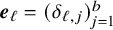
$\mathcal {S}_+=\{(\boldsymbol {e}_\ell ,\boldsymbol {n}_{\ell })_{\ell =1}^b\}$
 with
$\boldsymbol {e}_\ell \ (1\leq \ell \leq b)$
with
$\boldsymbol {e}_\ell \ (1\leq \ell \leq b)$
 the standard basis vectors for
$\mathbb Z^b$
the standard basis vectors for
$\mathbb Z^b$
 (i.e.,
$\boldsymbol {e}_\ell =(\delta _{\ell ,j})_{j=1}^b$
(i.e.,
$\boldsymbol {e}_\ell =(\delta _{\ell ,j})_{j=1}^b$
 ).
).
Remark 1.2. Theorem 1.1 readily generalizes to potentials V, which are given by finite Fourier series with both cosine and sine terms.
Remark 1.3. Note that we do not require the linear equation (1.4) to satisfy Anderson localization. However, linear Anderson localization does hold on a large subset of
$\mathcal W$
 (cf. [Reference BourgainBou07, Reference Jitomirskaya, Liu and ShiJLS20]).
1.1 Ideas of the proof
The multi-dimensional phase space, namely
$\boldsymbol {\theta }$
 being a vector instead of a scalar as in, for example, [Reference Shi and WangSW23] poses a major challenge. Diophantine properties of the eigenvalues of the linear Schrödinger operator (1.3) play an essential role in the proof. To
$O(\delta )$
being a vector instead of a scalar as in, for example, [Reference Shi and WangSW23] poses a major challenge. Diophantine properties of the eigenvalues of the linear Schrödinger operator (1.3) play an essential role in the proof. To
$O(\delta )$
 , this could be replaced by Diophantine properties of the potential
$V(\boldsymbol {n}\boldsymbol {\alpha }+\boldsymbol {\theta })$
, this could be replaced by Diophantine properties of the potential
$V(\boldsymbol {n}\boldsymbol {\alpha }+\boldsymbol {\theta })$
 at different lattice sites
$\boldsymbol {n}\in \mathbb Z^d$
at different lattice sites
$\boldsymbol {n}\in \mathbb Z^d$
 . We need to show that the values of the function at these chosen sites are, in some sense, linearly independent. This is, however, a priori, not obvious, since V is a given function on
$\mathbb R^d$
. We need to show that the values of the function at these chosen sites are, in some sense, linearly independent. This is, however, a priori, not obvious, since V is a given function on
$\mathbb R^d$
 . To prove linear independence, we use a generalized Wronskian approach and bound the determinant away from zero by carefully removing some
$(\boldsymbol {\alpha }, \boldsymbol {\theta })$
. To prove linear independence, we use a generalized Wronskian approach and bound the determinant away from zero by carefully removing some
$(\boldsymbol {\alpha }, \boldsymbol {\theta })$
 . This method is applicable to any trigonometric polynomials, generalizing the approach in [Reference Shi and WangSW23] for the cosine function on
$\mathbb R$
. This method is applicable to any trigonometric polynomials, generalizing the approach in [Reference Shi and WangSW23] for the cosine function on
$\mathbb R$
 . It is independent of the main body of the proof and could be of independent interest. Such arguments may be closely related to Diophantine approximations on manifold developed by Kleinbock and Margulis [Reference Kleinbock and MargulisKM98].
The other main ingredient of the proof is the application of Bourgain’s approach in the study of Anderson localization for linear quasi-periodic Schrödinger operators in d-dimensions [Reference BourgainBou07] (e.g., the
$\mathcal H$
 in (1.3)). Bourgain’s approach seems to be, so far, the only method available to deal with the d-dimensional phase space, that is,
$\boldsymbol {\theta } \in [0, 1]^d$
in (1.3)). Bourgain’s approach seems to be, so far, the only method available to deal with the d-dimensional phase space, that is,
$\boldsymbol {\theta } \in [0, 1]^d$
 ,
$d\geq 3$
,
$d\geq 3$
 . Among other innovations, it uses semi-algebraic geometry arguments (e.g., Yomdin-Gromov algebraic lemma) to control the resonances. The difficulty of d-dimensional phase space manifests as well in our paper, in that for the linear analysis, semi-algebraic geometry already seems indispensable to control the resonances; while in previous works, see [Reference Bourgain and WangBW08, Reference WangWan16, Reference Liu and WangLW24, Reference Shi and WangSW23], this role is filled by Diophantine properties. To control the resonances in time, we also need weak second Melnikov-type estimates. This could be readily obtained, similar to [Reference BourgainBou05a, Reference Bourgain and WangBW08, Reference Liu and WangLW24, Reference Shi and WangSW23]. In this paper, however, we have to overcome much more serious resonances in space (cf. Figure 1), which seems novel. The proof is then accomplished by doing multi-scale analysis with some new ideas.
The general problem discussed here is the persistence of quasi-periodic solutions of linear or integrable equations after Hamiltonian perturbation. This subject is closely related to the well-known “KAM theory” of invariant tori in smooth dynamical systems. Results along this line were first obtained by Kuksin [Reference KuksinKuk87] and Wayne [Reference WayneWay90], stimulating considerable progress, see, for example, [Reference Kuksin and PöschelKP96, Reference Chierchia and YouCY00, Reference Bambusi and GraffiBG01, Reference BourgainBou05b, Reference Eliasson and KuksinEK10, Reference Liu and YuanLY10, Reference Liu and YuanLY11, Reference Grébert and Thomann.GT11, Reference Berti, Biasco and ProcesiBBP13, Reference Procesi and ProcesiPP15, Reference Eliasson, Grébert and KuksinEGK16, Reference Baldi, Berti, Haus and MontaltoBBHM18, Reference Berti, Kappeler and MontaltoBKM18, Reference Cong, Liu, Shi and YuanCLSY18, Reference YuanYua21, Reference Berti, Hassainia and MasmoudiBHM23] to name but a few. The existence of quasi-periodic solutions can also be obtained using the direct Craig-Wayne-Bourgain method [Reference Craig and WayneCW93, Reference BourgainBou94, Reference BourgainBou98, Reference BourgainBou05a] (cf. [Reference Bourgain and WangBW08, Reference Berti and BolleBB13, Reference WangWan16, Reference He, Shi, Shi and YuanHSSY20, Reference WangWan21a, Reference WangWan21b, Reference Liu and WangLW24, Reference Shi and WangSW23, Reference Kachkovskiy, Liu and WangKLW24] for more recent results), which turns out to be more robust when dealing with multi-dimensional Hamiltonian PDEs (cf. Chapters 18–20 of [Reference BourgainBou05a]).
Finally, we mention the work [Reference YuanYua02] in which a KAM scheme was first developed to prove the existence of quasi-periodic solutions for some nonlinear discrete equations without external parameters (i.e., regarding the initial states as parameters). Later in [Reference Geng, You and ZhaoGYZ14], the authors also applied the KAM method to obtain the existence of quasi-periodic solutions for the nonlinear quasi-periodic Schrödinger equation on
$\mathbb Z$
 .
.
1.2 The nonlinear random Schrödinger equation
When the potential V, with
$V(\boldsymbol {n})=V(\boldsymbol {n} \boldsymbol {\alpha }+\boldsymbol {\theta })$
 , is replaced by a random potential, for example, with
$V(\boldsymbol {n})$
, is replaced by a random potential, for example, with
$V(\boldsymbol {n})$
 a family of independent identically distributed random variables (with the uniform distribution), it is known from [Reference Bourgain and WangBW08] that the nonlinear random Schrödinger equation

has large sets of Anderson localized states for small
$\varepsilon $
 and
$\delta $
and
$\delta $
 . When
$d=1$
. When
$d=1$
 , it is shown further in the important work [Reference Liu and WangLW24] that large sets of Anderson localized states persist for all
$\varepsilon \neq 0$
, it is shown further in the important work [Reference Liu and WangLW24] that large sets of Anderson localized states persist for all
$\varepsilon \neq 0$
 (similar results could be proven for the nonlinear wave equation). Recall that the first proof of the Anderson localization for the linear random Schrödinger equation

for small
$\varepsilon $
 was based on multi-scale-analysis-type Green’s function estimates developed in [Reference Fröhlich and SpencerFS83], see also [Reference Aizenman and MolchanovAM93].
It is generally believed that the linear random Schrödinger equation and the linear quasi-periodic Schrödinger equation should share common localization features in the perturbative regime, despite the quasi-periodic problems being more delicate and the results more difficult to obtain. The use of semi-algebraic geometry and Cartan’s Lemma [Reference Bourgain, Goldstein and SchlagBGS02, Reference BourgainBou07, Reference Jitomirskaya, Liu and ShiJLS20], for example, certainly renders the quasi-periodic issue more involved than that of the random, and this seems to continue to the nonlinear case, as mentioned earlier. Theorem 1.1 generalizes this circle of ideas to the nonlinear setting by providing a concrete example where the quasi-periodic and the random have indeed similar behavior.
1.3 Structure of the paper
In Section 2, we focus on the linear estimates, in the form of a large deviation theorem. The paper concludes by constructing the quasi-periodic in-time solutions in Section 3. The proof of the Diophantine-type estimates and some important lemmas on resolvent identities are presented in the Appendix.
2 Linear analysis
In this section, we investigate the properties of linearized operators on
$\mathbb Z^{b+d}$
 . Of particular importance is the large deviation theorem (LDT) for the corresponding Green’s functions.
2.1 The operator on the lattice
For a vector
$\boldsymbol {x}\in \mathbb R^r$
 , we denote by
$|\boldsymbol {x}|$
, we denote by
$|\boldsymbol {x}|$
 (resp.
$|\boldsymbol {x}|_2$
(resp.
$|\boldsymbol {x}|_2$
 ) the supremum norm (resp. the Euclidean norm). For an operator (or a matrix), we denote by
$\|\cdot \|$
) the supremum norm (resp. the Euclidean norm). For an operator (or a matrix), we denote by
$\|\cdot \|$
 its operator norm.
We define the lattice:

Let
$\mathcal {S}_+=\{(\boldsymbol {e}_\ell , \boldsymbol {n}_\ell )_{\ell =1}^b\}\subset \mathbb Z^{b+d}$
 and we identify
$ \mathcal {S}_+$
and we identify
$ \mathcal {S}_+$
 with
$\{(\boldsymbol {e}_\ell , \boldsymbol {n}_\ell )_{\ell =1}^b\}\times \{+\}\subset \mathbb Z^{b+d}_{\mathrm {pm}}$
with
$\{(\boldsymbol {e}_\ell , \boldsymbol {n}_\ell )_{\ell =1}^b\}\times \{+\}\subset \mathbb Z^{b+d}_{\mathrm {pm}}$
 . Similarly, let
$\mathcal {S}_-=\{(-\boldsymbol {e}_\ell , \boldsymbol {n}_\ell )_{\ell =1}^b\}\subset \mathbb Z^{b+d}$
. Similarly, let
$\mathcal {S}_-=\{(-\boldsymbol {e}_\ell , \boldsymbol {n}_\ell )_{\ell =1}^b\}\subset \mathbb Z^{b+d}$
 , which is then identified with
$\{(-\boldsymbol {e}_\ell , \boldsymbol {n}_\ell )_{\ell =1}^b\}\times \{-\}\subset \mathbb Z^{b+d}_{\mathrm {pm}}$
, which is then identified with
$\{(-\boldsymbol {e}_\ell , \boldsymbol {n}_\ell )_{\ell =1}^b\}\times \{-\}\subset \mathbb Z^{b+d}_{\mathrm {pm}}$
 . We let
$\mathcal S=\mathcal S_+\cup \mathcal S_-$
. We let
$\mathcal S=\mathcal S_+\cup \mathcal S_-$
 and
and

In the following, we study the operator on
$\mathbb Z^{b+d}_{\mathrm {pm},*}$
 the operator

where

and the operator S refers typically to the linearized operator of the nonlinear perturbation. So we may let S satisfy the following properties:
-
○ First
$$ \begin{align*}S:\ \ell^2(\mathbb Z^{b+d}_{\mathrm{pm}})\to \ell^2(\mathbb Z^{b+d}_{\mathrm{pm}})\end{align*} $$is a bounded self-adjoint operator.
-
○ For all $\boldsymbol {k},\boldsymbol {k}', \boldsymbol {k}''\in \mathbb Z^b$
,
$\boldsymbol {n},\boldsymbol {n}'\in \mathbb Z^d$
and
$\xi ,\xi '\in \{+, -\}$
, we have the Töplitz property in the
$\boldsymbol {k}$
-variable: $$ \begin{align*} S((\boldsymbol{k}'+\boldsymbol{k}, \boldsymbol{n}, \xi); (\boldsymbol{k}"+\boldsymbol{k}, \boldsymbol{n}', \xi'))=S((\boldsymbol{k}', \boldsymbol{n}, \xi ); (\boldsymbol{k}", \boldsymbol{n}', \xi')). \end{align*} $$
-
○ We have for some $C_2>0$
and
$\gamma \in (\frac 12, 10), $
$$ \begin{align*} |S((\boldsymbol{k}, \boldsymbol{n}, \xi); (\boldsymbol{k}', \boldsymbol{n}', \xi'))|\leq C_2(1+|\boldsymbol{k}-\boldsymbol{k}'|)^{C_2} e^{-\gamma|\boldsymbol{k}-\boldsymbol{k}'|-\gamma|\boldsymbol{n}|}\delta_{\boldsymbol{n},\boldsymbol{n}'}. \end{align*} $$






The frequency
$\boldsymbol {\omega }$
 satisfies

where
$C>0$
 and
$\boldsymbol {\omega }^{(0)}=\boldsymbol {\omega }^{(0)}(\boldsymbol {\alpha }, \boldsymbol {\theta })$
and
$\boldsymbol {\omega }^{(0)}=\boldsymbol {\omega }^{(0)}(\boldsymbol {\alpha }, \boldsymbol {\theta })$
 is defined in Theorem 1.1.
2.2 The (generalized) elementary regions on the lattice
For some technical reasons, we will introduce the definitions of elementary regions and generalized elementary regions on
$\mathbb Z^{b+d}$
 originating from [Reference Bourgain, Goldstein and SchlagBGS02, Reference BourgainBou07]. We refer to [Reference LiuLiu22] (cf. Section 2 in [Reference LiuLiu22]) for some important clarifications and improvements on those concepts.
Denote by
$\Lambda _N(\boldsymbol {x})$
 (
$\boldsymbol {x}\in \mathbb Z^{r},\ r=b+d,d$
(
$\boldsymbol {x}\in \mathbb Z^{r},\ r=b+d,d$
 ),
),

the cube of radius N centered at
$\boldsymbol {x}$
 . In particular, we write
$\Lambda _N=\Lambda _N(\boldsymbol {0})$
. In particular, we write
$\Lambda _N=\Lambda _N(\boldsymbol {0})$
 . For
$\Lambda \subset \mathbb Z^{r}$
. For
$\Lambda \subset \mathbb Z^{r}$
 , we define its diameter to be
$\mathrm {diam}\ \Lambda =\sup \limits _{\boldsymbol {x}, \boldsymbol {y}\in \Lambda }|\boldsymbol {x}-\boldsymbol {y}|$
, we define its diameter to be
$\mathrm {diam}\ \Lambda =\sup \limits _{\boldsymbol {x}, \boldsymbol {y}\in \Lambda }|\boldsymbol {x}-\boldsymbol {y}|$
 . For
$\boldsymbol {x}\in \mathbb Z^{r}$
. For
$\boldsymbol {x}\in \mathbb Z^{r}$
 and
$\boldsymbol {w}\in \mathbb R_+^{r}$
and
$\boldsymbol {w}\in \mathbb R_+^{r}$
 , let
$R_{\boldsymbol {w}}(\boldsymbol {x})=\{\boldsymbol {y}\in \mathbb Z^{r}:\ |y_\ell -x_\ell |\leq w_l , \, 1\leq \ell \leq r\}$
, let
$R_{\boldsymbol {w}}(\boldsymbol {x})=\{\boldsymbol {y}\in \mathbb Z^{r}:\ |y_\ell -x_\ell |\leq w_l , \, 1\leq \ell \leq r\}$
 denote the rectangle.
A generalized elementary region is defined to be a set
$\Lambda $
 of the form

where
$\boldsymbol {z}\in \mathbb Z^{r}$
 is arbitrary. The size of a generalized elementary region is simply its diameter. The set of all generalized elementary regions of size at most M will be denoted by
$\mathcal {E}_M$
is arbitrary. The size of a generalized elementary region is simply its diameter. The set of all generalized elementary regions of size at most M will be denoted by
$\mathcal {E}_M$
 .
.
An elementary region
$Q_N$
 of size N and centered at
$\boldsymbol {0}$
of size N and centered at
$\boldsymbol {0}$
 is one of the following regions

where
$\square _\ell \in \{<,>, \emptyset \}$
 and at least two
$\square _\ell $
and at least two
$\square _\ell $
 ’s are not
$\emptyset .$
’s are not
$\emptyset .$
 Denote by
$\mathcal {ER}_{\boldsymbol {0}}(N)$
Denote by
$\mathcal {ER}_{\boldsymbol {0}}(N)$
 the set of all elementary regions of size N and centered at
$\boldsymbol {0}$
the set of all elementary regions of size N and centered at
$\boldsymbol {0}$
 . Let
. Let

Let
$\mathcal E_{M}^{L}$
 denote the set of all M-size generalized elementary regions of width at least
$L\leq M$
denote the set of all M-size generalized elementary regions of width at least
$L\leq M$
 , namely,
$\Lambda \in \mathcal {E}_{M}^{L}$
, namely,
$\Lambda \in \mathcal {E}_{M}^{L}$
 iff
$\Lambda \in \mathcal {E}_{M}$
iff
$\Lambda \in \mathcal {E}_{M}$
 and, for any
$\boldsymbol {x}\in \Lambda , 0<L'<L$
and, for any
$\boldsymbol {x}\in \Lambda , 0<L'<L$
 , there is some
$\Lambda '\in \mathcal {ER}(L')$
, there is some
$\Lambda '\in \mathcal {ER}(L')$
 so that
$\boldsymbol {x}\in \Lambda '\subset \Lambda $
so that
$\boldsymbol {x}\in \Lambda '\subset \Lambda $
 ,
$\mathrm {dist}(\boldsymbol {x}, \Lambda \setminus \Lambda ')\geq L'/2$
,
$\mathrm {dist}(\boldsymbol {x}, \Lambda \setminus \Lambda ')\geq L'/2$
 , where
$\mathrm {dist} (\cdot , \cdot )$
, where
$\mathrm {dist} (\cdot , \cdot )$
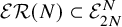
 is induced by the supremum norm. So we have
$\mathcal {ER}(N) \subset \mathcal E_{2N}^{N}$
is induced by the supremum norm. So we have
$\mathcal {ER}(N) \subset \mathcal E_{2N}^{N}$
 .
.
With a slight abuse of notation, we also use
$\mathcal {ER}_{\boldsymbol {0}}(N), \mathcal {ER}(N), \mathcal E_N, \mathcal E_N^L , \Lambda _N(\boldsymbol {x}),\ \Lambda _N$
 to denote
$\mathcal {ER}_{\boldsymbol {0}}(N)\times \{+,-\}, \mathcal {ER}(N)\times \{+,-\}, \mathcal E_N\times \{+,-\}, \mathcal E_N^L \times \{+,-\}, \Lambda _N(\boldsymbol {x})\times \{+,-\}, \Lambda _N\times \{+,-\}$
to denote
$\mathcal {ER}_{\boldsymbol {0}}(N)\times \{+,-\}, \mathcal {ER}(N)\times \{+,-\}, \mathcal E_N\times \{+,-\}, \mathcal E_N^L \times \{+,-\}, \Lambda _N(\boldsymbol {x})\times \{+,-\}, \Lambda _N\times \{+,-\}$
 . Similarly, for any
$\Lambda \subset \mathbb Z^r$
. Similarly, for any
$\Lambda \subset \mathbb Z^r$
 , denote by
$R_\Lambda $
, denote by
$R_\Lambda $
 the restriction to
$\Lambda \times \{+,-\}$
the restriction to
$\Lambda \times \{+,-\}$
 .
.
2.3 Green’s functions and LDE
We now define Green’s functions on subsets of
$\mathbb Z_{\mathrm {pm},*}^{b+d}$
 . Let
$\Lambda \subset \mathbb Z_{\mathrm {pm},*}^{b+d}$
. Let
$\Lambda \subset \mathbb Z_{\mathrm {pm},*}^{b+d}$
 be a nonempty set,
$R_\Lambda $
be a nonempty set,
$R_\Lambda $
 the restriction operator to
$\Lambda $
the restriction operator to
$\Lambda $
 , and define the
$(\# \Lambda ) \times (\#\Lambda )$
, and define the
$(\# \Lambda ) \times (\#\Lambda )$
 matrix:

where
$H(\sigma )$
 is defined by (2.1). Define the Green’s function to be (if it exists)

Before addressing the LDT for Green’s functions, let us first give the definition of large deviation estimates (LDE):
Definition 2.1 (LDE)
Let
$\rho>0$
 ,
$0<\gamma '<\gamma $
,
$0<\gamma '<\gamma $
 and
$M\in \mathbb {N}$
and
$M\in \mathbb {N}$
 . We say
${H}(\sigma )$
. We say
${H}(\sigma )$
 defined by (2.1) satisfies the
$(\rho , \gamma ',M)$
defined by (2.1) satisfies the
$(\rho , \gamma ',M)$
 -LDE if there exists a set
$\Sigma _M\subset \mathbb R$
-LDE if there exists a set
$\Sigma _M\subset \mathbb R$
 with
with

so that for
$\sigma \notin \Sigma _M$
 the following estimates hold: If
$\Lambda \in (\boldsymbol {0},\boldsymbol {n})+ \mathcal {ER}_{\boldsymbol {0}}(M)$
the following estimates hold: If
$\Lambda \in (\boldsymbol {0},\boldsymbol {n})+ \mathcal {ER}_{\boldsymbol {0}}(M)$
 satisfies
$|\boldsymbol {n}|\leq 10M$
satisfies
$|\boldsymbol {n}|\leq 10M$
 , then

where
$\boldsymbol {x}=(\boldsymbol {k}',\boldsymbol {n}'), \boldsymbol {x}'=(\boldsymbol {k}'',\boldsymbol {n}'')$
 .
.
We will show in this section that the
$(\rho , \frac {\gamma }{2},N)$
 -LDE hold for some small

and all
$N\gg 1$
 , under certain nonresonant conditions on
$\boldsymbol {\alpha }, \boldsymbol {\theta }$
, under certain nonresonant conditions on
$\boldsymbol {\alpha }, \boldsymbol {\theta }$
 and
$\boldsymbol {\omega }$
and
$\boldsymbol {\omega }$
 . This leads to the LDT, Theorem 2.11, below. Since we view
$\boldsymbol {\omega }$
. This leads to the LDT, Theorem 2.11, below. Since we view
$\boldsymbol {\omega }$
 as an
$O(\delta )$
as an
$O(\delta )$
 perturbation of
$\boldsymbol {\omega }^{(0)}$
perturbation of
$\boldsymbol {\omega }^{(0)}$
 , the properties of
$\boldsymbol {\omega }^{(0)}$
, the properties of
$\boldsymbol {\omega }^{(0)}$
 become essential in the proof of LDT. So, in the following, we first establish nonresonant properties (called Diophantine estimates) of
$\boldsymbol {\omega }^{(0)}$
become essential in the proof of LDT. So, in the following, we first establish nonresonant properties (called Diophantine estimates) of
$\boldsymbol {\omega }^{(0)}$
 . Then the proof of LDT will follow from a multi-scale analysis scheme in the spirit of [Reference Bourgain, Goldstein and SchlagBGS02, Reference BourgainBou05a, Reference BourgainBou07].
2.4 Diophantine estimates
Recall that

The main purpose of this section is to obtain lower bounds on

under certain restrictions on
$(\boldsymbol {\alpha }, \boldsymbol {\theta })$
 . As mentioned in the Introduction, due to the d-dimensional phase space, such Diophantine-type estimates are highly nontrivial. We use a generalized Wronskian approach and work out the details in the Appendix (cf. Theorem A.2 and Corollary A.4). These estimates can be read independently, and are key to the existence of quasi-periodic solutions to the nonlinear equation.
Applying Corollary A.4 then leads to
Theorem 2.2. There exist some
$0<c_1=c_1(b,d,K,V)<\frac {1}{100b}, C_1=C_1(b,d, K, V)>1$
 such that, if
$0<\varepsilon +\delta \leq \delta _0(b,d,K,V,\max \limits _{1\leq \ell \leq b}|\boldsymbol {n}_\ell |)\ll 1$
such that, if
$0<\varepsilon +\delta \leq \delta _0(b,d,K,V,\max \limits _{1\leq \ell \leq b}|\boldsymbol {n}_\ell |)\ll 1$
 , then there is some
$\mathcal M \subset [0, 1]^{2d}$
, then there is some
$\mathcal M \subset [0, 1]^{2d}$
 satisfying

so that the following properties hold true for
$(\boldsymbol {\alpha }, \boldsymbol {\theta })\in \mathcal M$
 and
$L_{\varepsilon ,\delta }:=100(\varepsilon +\delta )^{-c_1}$
and
$L_{\varepsilon ,\delta }:=100(\varepsilon +\delta )^{-c_1}$
 .
.
-
(1) For all $\log \frac {1}{\varepsilon +\delta }\leq L\leq L_{\varepsilon ,\delta }$
and all
$(\boldsymbol {k},\boldsymbol {n})\in \Lambda _{L}\setminus \mathcal S,$
we have (2.5) $$ \begin{align} \min_{\xi=\pm1}|\xi\boldsymbol{k}\cdot\boldsymbol{\omega}^{(0)}+\mu_{\boldsymbol{n}}|>L^{-C_1}. \end{align} $$
-
(2) We have for any $\xi =\pm 1,$
(2.6) $$ \begin{align} \sup_{\sigma\in\mathbb R}\#\left\{(\boldsymbol{k},\boldsymbol{n})\in \Lambda_{L_{\varepsilon,\delta}}:\ |\xi(\sigma+\boldsymbol{k}\cdot\boldsymbol{\omega}^{(0)})+\mu_{\boldsymbol{n}}|<\frac{(\varepsilon+\delta)^{\frac{1}{8b}}}{4}\right\}\leq b. \end{align} $$




Remark 2.3. The estimate in (1) plays an essential role in the initial iteration steps for the nonlinear analysis. The conclusion (2) of this theorem will be only used in the proof of intermediate scales LDE.
Proof. The proof is similar to that in [Reference Shi and WangSW23]. First, the measure estimate (2.4) is a consequence of Corollary A.4. Next, the inequality (2.5) in (1) follows directly from (iii) of Corollary A.4.
So, it suffices to establish (2.6) of (2). We prove it by the contradiction. Without loss of generality, we consider the case
$\xi =+1$
 . Assume that there are
$b+1$
. Assume that there are
$b+1$
 distinct
$\{(\boldsymbol {k}_\ell , \boldsymbol {n}_{\ell }')\}_{1\leq \ell \leq b+1}$
distinct
$\{(\boldsymbol {k}_\ell , \boldsymbol {n}_{\ell }')\}_{1\leq \ell \leq b+1}$
 satisfying

We claim that all
$\boldsymbol {k}_{\ell }$
 (
$1\leq \ell \leq b+1$
(
$1\leq \ell \leq b+1$
 ) are distinct. Actually, if there are
$\boldsymbol {k}_{\ell _1}=\boldsymbol {k}_{\ell _2}$
) are distinct. Actually, if there are
$\boldsymbol {k}_{\ell _1}=\boldsymbol {k}_{\ell _2}$
 for some
$1\leq \ell _1\neq \ell _2\leq b+1$
for some
$1\leq \ell _1\neq \ell _2\leq b+1$
 , then it must be that
$\boldsymbol {n}_{\ell _1}'\neq \boldsymbol {n}_{\ell _2}'$
, then it must be that
$\boldsymbol {n}_{\ell _1}'\neq \boldsymbol {n}_{\ell _2}'$
 . As a result, we obtain using (2.7) that

which contradicts (i) of Corollary A.4. Next, we claim that
$\{\boldsymbol {n}_{\ell }'\}_{1\leq \ell \leq b+1}\subset \{\boldsymbol {n}_{\ell }\}_{1\leq \ell \leq b}.$
 In fact, if
$\boldsymbol {n}_{\ell _1}'\notin \{\boldsymbol {n}_{\ell }\}_{1\leq \ell \leq b}$
In fact, if
$\boldsymbol {n}_{\ell _1}'\notin \{\boldsymbol {n}_{\ell }\}_{1\leq \ell \leq b}$
 for some
$1\leq \ell _1\leq b+1$
for some
$1\leq \ell _1\leq b+1$
 , we can assume that there is
$\ell _2\neq \ell _1$
, we can assume that there is
$\ell _2\neq \ell _1$
 so that
$\boldsymbol {n}_{\ell _2}'\neq \boldsymbol {n}_{\ell _1}'$
so that
$\boldsymbol {n}_{\ell _2}'\neq \boldsymbol {n}_{\ell _1}'$
 . Otherwise, we may have

which contradicts (ii) of Corollary A.4, since
$\boldsymbol {k}_{\ell _1}\neq \boldsymbol {k}_{\ell _2}$
 as claimed above. So we obtain for some
$\ell _2\neq \ell _1$
as claimed above. So we obtain for some
$\ell _2\neq \ell _1$
 and
$1\leq \ell _2\leq b+1$
and
$1\leq \ell _2\leq b+1$
 with
$\boldsymbol {n}_{\ell _2}'\neq \boldsymbol {n}_{\ell _1}'$
with
$\boldsymbol {n}_{\ell _2}'\neq \boldsymbol {n}_{\ell _1}'$
 that
that

which contradicts (iv) of Corollary A.4. So it suffices to assume
$\{\boldsymbol {n}_{\ell }'\}_{1\leq \ell \leq b+1}\subset \{\boldsymbol {n}_{\ell }\}_{1\leq \ell \leq b}.$
 However, in this case, we have by the pigeonhole principle that there are
$1\leq \ell _1\neq \ell _2\leq b+1$
However, in this case, we have by the pigeonhole principle that there are
$1\leq \ell _1\neq \ell _2\leq b+1$
 so that
$\boldsymbol {n}_{\ell _1}'=\boldsymbol {n}_{\ell _2}'$
so that
$\boldsymbol {n}_{\ell _1}'=\boldsymbol {n}_{\ell _2}'$
 . Then we get

which contradicts (ii) of Corollary A.4 as shown above. This proves (2.6).
2.5 Bourgain’s geometric lemma
To proceed with the analysis, we will also need Anderson localization-type properties for the linear quasi-periodic Schrödinger operator
$\mathcal H$
 in (1.3), namely,

This was proven by Bourgain in the remarkable work [Reference BourgainBou07], where he established Anderson localization for general quasi-periodic Schrödinger operators on
$\mathbb Z^d$
 with nondegenerate analytic potentials on
$\mathbb {T}^d$
with nondegenerate analytic potentials on
$\mathbb {T}^d$
 (identified with
$[0,1]^d$
(identified with
$[0,1]^d$
 ). This result was later significantly extended by Jitomirskaya-Liu-Shi [Reference Jitomirskaya, Liu and ShiJLS20] (cf. also [Reference ShiShi22, Reference LiuLiu22]) to potentials on
$\mathbb {T}^b$
). This result was later significantly extended by Jitomirskaya-Liu-Shi [Reference Jitomirskaya, Liu and ShiJLS20] (cf. also [Reference ShiShi22, Reference LiuLiu22]) to potentials on
$\mathbb {T}^b$
 for
$b\geq d.$
for
$b\geq d.$

In the present paper, due to the d-dimensional phase space, we need to apply Bourgain’s arguments. Using short-range property of S in the
$\boldsymbol {n}$
 -variable, Bourgain’s geometric lemma is made available to handle LDE for Green’s functions at large scales. This is a main new aspect not present in [Reference Shi and WangSW23]. The general scheme is similar to that in Chapter 19 of [Reference BourgainBou05a], where Bourgain made a great breakthrough and first proved the existence of quasi-periodic solutions for the nonlinear Schrödinger equation on arbitrarily dimensional torus (a KAM theorem was later established by Eliasson-Kuksin in an important paper [Reference Eliasson and KuksinEK10]). Among others, Bourgain [Reference BourgainBou05a] employed heavily the separation property of eigenvalues of the Laplace operator on the higher dimensional torus, while the separation property is missing in the present setting (indeed, the spectrum of
$\mathcal H$
-variable, Bourgain’s geometric lemma is made available to handle LDE for Green’s functions at large scales. This is a main new aspect not present in [Reference Shi and WangSW23]. The general scheme is similar to that in Chapter 19 of [Reference BourgainBou05a], where Bourgain made a great breakthrough and first proved the existence of quasi-periodic solutions for the nonlinear Schrödinger equation on arbitrarily dimensional torus (a KAM theorem was later established by Eliasson-Kuksin in an important paper [Reference Eliasson and KuksinEK10]). Among others, Bourgain [Reference BourgainBou05a] employed heavily the separation property of eigenvalues of the Laplace operator on the higher dimensional torus, while the separation property is missing in the present setting (indeed, the spectrum of
$\mathcal H$
 may contain an interval).
We start with introducing the definition of semi-algebraic sets.
Definition 2.4. A set
$X\subset \mathbb {R}^r$
 is called semi-algebraic if it is a finite union of sets defined by a finite number of polynomial equalities and inequalities. More precisely, let
$\{P_1,\cdots ,P_k\}\subset \mathbb {R}[x_1,\cdots ,x_r]$
is called semi-algebraic if it is a finite union of sets defined by a finite number of polynomial equalities and inequalities. More precisely, let
$\{P_1,\cdots ,P_k\}\subset \mathbb {R}[x_1,\cdots ,x_r]$
 be a family of real polynomials whose degrees are bounded by p. A (closed) semi-algebraic set
${X}$
be a family of real polynomials whose degrees are bounded by p. A (closed) semi-algebraic set
${X}$
 is given by an expression

where
$\mathcal {K}_s\subset \{1,\cdots ,k\}$
 and
$\varsigma _{s\ell }\in \{\geq ,\leq ,=\}$
and
$\varsigma _{s\ell }\in \{\geq ,\leq ,=\}$
 . Then we say that
${X}$
. Then we say that
${X}$
 has degree at most
$kp$
has degree at most
$kp$
 . In fact, the degree of
${X}$
. In fact, the degree of
${X}$
 which is denoted by
$\deg {X}$
which is denoted by
$\deg {X}$
 , means the smallest
$kp$
, means the smallest
$kp$
 over all representations as in (2.8).
Denote by
$\mathcal {ER}_{\mathbb Z^d}(M)$
 (resp.
$\mathcal {ER}_{\mathbb Z^d, \boldsymbol {0}}(M)$
(resp.
$\mathcal {ER}_{\mathbb Z^d, \boldsymbol {0}}(M)$
 ) the set of all M-size elementary regions on
$\mathbb Z^d$
) the set of all M-size elementary regions on
$\mathbb Z^d$
 (resp. centered at
$\boldsymbol {0}$
(resp. centered at
$\boldsymbol {0}$
 ). We have
Lemma 2.5 (cf. the Claim (page 694) in [Reference BourgainBou07] and Theorem 2.7 in [Reference Jitomirskaya, Liu and ShiJLS20])
There are small constants
$0<\kappa _1<\kappa _2<1$
 depending only on d so that the following holds true. For
$0<\varepsilon \leq \varepsilon _0(V,d)\ll 1 $
depending only on d so that the following holds true. For
$0<\varepsilon \leq \varepsilon _0(V,d)\ll 1 $
 and
$N\geq N_1:=10^{-\frac {32}{\kappa _1^2}}\log ^{\frac {4}{\kappa _1}}(\log \frac 1\varepsilon )$
and
$N\geq N_1:=10^{-\frac {32}{\kappa _1^2}}\log ^{\frac {4}{\kappa _1}}(\log \frac 1\varepsilon )$
 , there is a semi-algebraic set
$\mathcal {A}_N\subset [0,1]^d$
, there is a semi-algebraic set
$\mathcal {A}_N\subset [0,1]^d$
 satisfying

so that the following properties hold true for
$\boldsymbol {\alpha }\in \mathcal {A}_N.$

-
(1) For all $E\in \mathbb R$
and all
$\boldsymbol {\theta }\in [0,1]^d$
, there is
$L\in [N^{\kappa _1}, N^{\kappa _2}]$
so that, for all
$Q\in \mathcal {ER}_{\mathbb Z^d}(L_1) $
satisfying
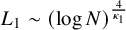
$L_1\sim (\log N)^{\frac {4}{\kappa _1}}$
and $$ \begin{align*}Q\subset [-L,L]^d\setminus[-L^{\frac{1}{10d}}, L^{\frac{1}{10d}}]^d,\end{align*} $$one has
$$ \begin{align*} \|\mathcal{H}^{-1}_{Q}(E;\boldsymbol{\theta})\|&\leq e^{\sqrt{L_1}},\\ |\mathcal{H}^{-1}_{Q}(E;\boldsymbol{\theta})(\boldsymbol{n}; \boldsymbol{n}')|&\leq e^{-\frac12|\log\varepsilon|\cdot|\boldsymbol{n}-\boldsymbol{n}'|}\ \mathrm{for}\ |\boldsymbol{n}-\boldsymbol{n}'|\geq L_1^{\frac 89}, \end{align*} $$where
$$ \begin{align*} \mathcal{H}_{Q}(E;\boldsymbol{\theta})&=R_{Q}\left(\varepsilon\Delta+V(\boldsymbol{\theta}+\boldsymbol{n}\boldsymbol{\alpha})\delta_{\boldsymbol{n}, \boldsymbol{n}'}\right)R_{Q}-E\\ &:=\mathcal{L}_{Q}(\boldsymbol{\theta})-E. \end{align*} $$
-
(2) There is some $\Theta _N=\Theta _N(\boldsymbol {\alpha })\subset [0,1]^d$
satisfying $$ \begin{align*}\mathrm{meas}([0, 1]^d\setminus\Theta_N)\leq e^{-N^{\frac{\kappa_1}{4}}}\end{align*} $$so that, if $\boldsymbol {\theta }\in \Theta _N$
, then one has for all
$\Lambda \in \mathcal {ER}_{\mathbb Z^d, \boldsymbol {0}}(N),$
$$ \begin{align*} \|\mathcal{H}^{-1}_{\Lambda}(\boldsymbol{\alpha}, \boldsymbol{\theta})\|&\leq e^{\sqrt{N}},\\ |\mathcal{H}^{-1}_{\Lambda}(\boldsymbol{\alpha}, \boldsymbol{\theta})(\boldsymbol{n}; \boldsymbol{n}')|&\leq e^{-\frac12|\log\varepsilon|\cdot|\boldsymbol{n}-\boldsymbol{n}'|}\ \mathrm{for}\ |\boldsymbol{n}-\boldsymbol{n}'|\geq {N^{\frac 89}}. \end{align*} $$
Denote
(2.9) $$ \begin{align} \nonumber&\mathcal{A}=\bigcap_{N\geq N_1}\mathcal{A}_N,\ \tilde\Theta_N(\boldsymbol{\alpha})=\bigcap_{|\boldsymbol{n}|\leq e^{N^{\frac{\kappa_1}{5}}}}\left\{\boldsymbol{\theta}:\ \boldsymbol{\theta}+\boldsymbol{n}\boldsymbol{\alpha}\in\Theta_N\right\}, \\ &\mathcal W'=\left\{(\boldsymbol{\alpha}, \boldsymbol{\theta})\in[0,1]^{2d}:\ \boldsymbol{\alpha}\in\mathcal A,\ \boldsymbol{\theta}\in\bigcap_{N\geq N_1}\tilde\Theta_N(\boldsymbol{\alpha})\right\}. \end{align} $$
Then
(2.10) $$ \begin{align} \mathrm{meas}(\mathcal W')\geq 1-\log^{-c}\frac1\varepsilon. \end{align} $$












Remark 2.6. In this lemma, the constants
$\kappa _1, \kappa _2$
 correspond to
$c_3, c_4$
correspond to
$c_3, c_4$
 of [Reference Jitomirskaya, Liu and ShiJLS20], respectively. Originally, the off-diagonal exponential decay distance (cf., e.g., decay estimates in (2) of Lemma 2.5) in [Reference BourgainBou07, Reference Jitomirskaya, Liu and ShiJLS20] is
$|\boldsymbol {n}-\boldsymbol {n}'|\geq \frac {N}{10}$
of [Reference Jitomirskaya, Liu and ShiJLS20], respectively. Originally, the off-diagonal exponential decay distance (cf., e.g., decay estimates in (2) of Lemma 2.5) in [Reference BourgainBou07, Reference Jitomirskaya, Liu and ShiJLS20] is
$|\boldsymbol {n}-\boldsymbol {n}'|\geq \frac {N}{10}$
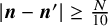 . However, it can be improved to the present sublinear scale
$N^{\frac 89}.$
. However, it can be improved to the present sublinear scale
$N^{\frac 89}.$
 This issue is important for the nonlinear analysis, and can be resolved with little effort, cf. Remark B.7 and Remark B.4 in the Appendix for more details.
Remark 2.7. The proof of this lemma is based on analysis of semi-algebraic sets (cf. [Reference BourgainBou07, Reference Jitomirskaya, Liu and ShiJLS20]), and applies to general nondegenerate analytic potentials.
Remark 2.8. We mention that the set
$\mathcal W$
 on which Theorem 1.1 holds satisfies

where
$\mathcal M$
 is the set on which the Diophantine estimates in Theorem 2.2 hold, and
$\mathcal W'$
is the set on which the Diophantine estimates in Theorem 2.2 hold, and
$\mathcal W'$
 is defined by (2.9). So, we have

as shown in Theorem 1.1. For
$(\boldsymbol {\alpha }, \boldsymbol {\theta })\in \mathcal W$
 , the conclusion in (2) plays an essential role in the nonlinear analysis.
Proof. It suffices to establish the measure bounds. The proof is a small modification of that of Theorem 4.1 in [Reference Jitomirskaya, Liu and ShiJLS20] (cf. pages 475–476). Indeed, the only difference is that we will apply Theorem 3.7 in [Reference Jitomirskaya, Liu and ShiJLS20] starting from
$N_1=10^{-\frac {32}{\kappa _1^2}}\log ^{\frac {4}{\kappa _1}}(\log \frac 1\varepsilon )$
 rather than
$\log \log \frac 1\varepsilon $
rather than
$\log \log \frac 1\varepsilon $
 as in [Reference Jitomirskaya, Liu and ShiJLS20]. This change makes sense since the large deviation estimates in [Reference Jitomirskaya, Liu and ShiJLS20] hold for the initial scales of
$N_0(V,d)\leq N\leq N_2:=\frac {1}{10}\log ^2\frac 1 \varepsilon $
as in [Reference Jitomirskaya, Liu and ShiJLS20]. This change makes sense since the large deviation estimates in [Reference Jitomirskaya, Liu and ShiJLS20] hold for the initial scales of
$N_0(V,d)\leq N\leq N_2:=\frac {1}{10}\log ^2\frac 1 \varepsilon $
 (via the Neumann series argument), and for
$f(x)=e^{x^{\frac {\kappa _1}{4}}},$
(via the Neumann series argument), and for
$f(x)=e^{x^{\frac {\kappa _1}{4}}},$
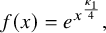

This modification then leads to the following measure estimate:

For the proof of (2.10), it follows directly from applying Fubini’s theorem and

2.6 Large deviation theorem
In this section, we establish that the LDE (cf. Definition 2.1) hold for all sufficiently large scales by a multi-scale analysis. From (2.2), however, the variation of the frequency,
$\boldsymbol {\omega }$
 is only
$O(\delta )$
is only
$O(\delta )$
 and not
$O(1)$
and not
$O(1)$
 , hence as we will see shortly, the proof of LDT will be accomplished in three steps instead of the usual two:
-
○ The first step deals with the small scales, for which we establish LDE for all $\boldsymbol {\omega }\in \Omega $
and scales $$ \begin{align*}N_0\leq N \leq 10^{-\frac{1}{\rho}}\log^{\frac{1}{\rho}} \frac{1}{\varepsilon+\delta},\end{align*} $$for some $\rho>0.$
In this step, we only use the Neumann series argument, which leads to the above scales (cf. Lemma 2.15).
-
○ Next, we establish intermediate scales LDE, that is, scales in the range
$$ \begin{align*}10^{-\frac{1}{\rho}}\log^{\frac{1}{\rho}} \frac{1}{\varepsilon+\delta}\leq N\leq (\varepsilon+\delta)^{-c_1}\end{align*} $$for all $\boldsymbol {\omega }\in \Omega $
, where
$c_1$
is defined in Theorem 2.2. Note that Theorem 2.2 is available in the above interval of scales. The proof of such intermediate scales LDE is based on preparation type theorem together with clustering properties of the spectrum of the diagonal matrix
$D(0)$
(cf. (2.6), Theorem 2.2).Remark 2.9. The intermediate scales are needed here because for a fixed $(\boldsymbol {\alpha },\boldsymbol {\theta })$
, hence fixed
$\boldsymbol {\omega }^{(0)}$
,
$\boldsymbol {\omega }$
only varies in an interval of size
$O(\delta )$
, see (2.2), as mentioned above. Consequently, there is a gap in the range of scales before Bourgain-type analysis becomes applicable. Fortunately, the Diophantine estimates for
$(\boldsymbol {\alpha },\boldsymbol {\theta })\in \mathcal M$
can control the resonances directly as in (2.6), leading to LDE for the range of scales in the gap, which we term the intermediate scales. -
○ For the large scales (i.e., $N>(\varepsilon +\delta )^{-c_1}$
) LDE, we will apply matrix-valued Cartan’s lemma and semi-algebraic sets theory of [Reference Bourgain, Goldstein and SchlagBGS02, Reference BourgainBou07]. Of particular importance is Bourgain’s geometric lemma (cf. Lemma 2.5). This step requires both the Diophantine condition and the so-called weak second Melnikov’s condition on
$\boldsymbol {\omega }.$
To be coherent, since the variation in $\boldsymbol {\omega }$
is only
$O(\delta )$
, the excised measure in
$\Omega $
needs to be less than
$\delta ^b$
. So we make a particular choice of the exponent and impose the following Diophantine condition: (2.12) $$ \begin{align} \nonumber&\ \ \ \mathrm{DC}_{\boldsymbol{\omega}}(N)\\ &=\left\{\boldsymbol{\omega}\in\Omega:\ |\boldsymbol{k}\cdot\boldsymbol{\omega}|\geq e^{-N^{\rho^4}} \ \mathrm{for}\ \forall\ 0<|\boldsymbol{k}|\leq 100N^2\right\}. \end{align} $$
Then we have for $\varepsilon \leq \delta $
, (2.13) $$ \begin{align} \mathrm{meas}\ \left(\Omega\setminus\left(\bigcap_{N>(\varepsilon+\delta)^{-c_1} }\mathrm{DC}_{\boldsymbol{\omega}}(N)\right)\right) \ll\delta^b. \end{align} $$
The weak second Melnikov’s condition is imposed in order to restrict the time $\boldsymbol {k}$
-direction where resonances could possibly occur. This greatly reduces the number of resonances, and paves the way for the application of Lemma 2.25.Remark 2.10. The condition on the size of $\varepsilon $
relative to
$\delta $
stems again from the modulation in
$\boldsymbol {\omega }$
being
$O(\delta )$
, while the excised measure depends on both
$\varepsilon $
and
$\delta $
, as we will see in the proofs. This also ensures, in addition, that the amplitude-frequency map:
$\boldsymbol {a}\to \boldsymbol {\omega }(\boldsymbol {a})$
is nondegenerate in the nonlinear analysis, so that we may indeed vary
$\boldsymbol {\omega }$
in the linear analysis.





Before stating the LDT, let us summarize various parameters and the relation between
$\varepsilon , \delta $
 .
.
-
○ Throughout this paper, we first fix constants
$$ \begin{align*}\kappa_1=\kappa_1(d), \kappa_2=\kappa_2(d)\in(0,1)\end{align*} $$given in Bourgain’s geometric lemma (cf. Lemma 2.5).
-
○ The most important parameter $\rho>0$
is then fixed so that it depends only on
$b,d$
and satisfies (2.14) $$ \begin{align} \rho=c_2 \kappa_1\leq \frac{\kappa_1}{10^4(b+d)^2}, \end{align} $$where $c_2=c_2(b,d)$
is given by Lemma 2.22.
-
○ The parameters
$$ \begin{align*}0<c_1=c_1(b,d, K, V)<\frac{1}{100b}, \ C_1=C_1(b,d,K,V)>1\end{align*} $$are fixed, which appear in the Diophantine estimates (cf. Theorem 2.2). Also, the parameter $c_1$
is the power-law exponent of the upper bound of intermediate scales.
-
○ Fix
$$ \begin{align*}\kappa=\frac12\min\left\{\vartheta, \ \frac{1}{10}\right\}\leq \frac{1}{20},\end{align*} $$where $\vartheta>0$
is an absolute constant appearing in the coupling lemma of [Reference LiuLiu22] (cf. Lemma B.3). Then
$\kappa $
(cf. (2.35)) describes the changes of off-diagonal exponential decay rates of Green’s functions along the multi-scale iterations.
-
○ For convenience, we assume the decay rate of S satisfies $\gamma \in (\frac 12, 10)$
. It turns out that the
$(\rho , \gamma _{\infty }, N)$
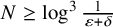
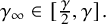
-LDE hold true for all
$N\geq \log ^{3}\frac {1}{\varepsilon +\delta }$
and for some
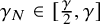
$\gamma _\infty \in [\frac \gamma 2, \gamma ].$
The constant
$C_2>0$
is the power-law index in
$S.$
-
○ With these parameters having been fixed, we aim to find
$$ \begin{align*}\delta_0=\delta_0(b, d, K, V, \max\limits_{1\leq \ell\leq b}|\boldsymbol{n}_\ell|, \kappa_1, \kappa_2, \rho, c_1, C_2)>0,\end{align*} $$so that, if $0<\varepsilon +\delta \leq \delta _0$
, then LDT can be established. Since we will use the multi-scale analysis method to prove LDT, various conditions on
$\delta _0$
are required, and it is unclear a priori if such restrictions are meaningful. Fortunately, we will divide the LDT proof into 3 steps, and at each step, we can find a desired
$\delta _\ell $
(
$\ell =1,2,3$
). Finally, it suffices to take
$\delta _0=\min \{\delta _1, \delta _2, \delta _3\}.$
-
○ As we will see later, we further assume $\delta \leq \log ^{-1}\frac 1\varepsilon $
when proving large scales LDE.












Let
$\rho , \kappa _1, \kappa _2, c_1, \gamma , C_2$
 be fixed as above. We have
Theorem 2.11 (LDT)
There is some

so that the following holds true for
$0<\varepsilon +\delta \leq \delta _0.$

-
(1) For $\log ^{3}\frac {1}{\varepsilon +\delta }< N\leq 10^{-\frac 1\rho }\log ^{\frac {1}{\rho }}\frac {1}{\varepsilon +\delta },$
the
$(\rho , \gamma _N, N)$
-LDE hold true for all
$(\boldsymbol {\alpha }, \boldsymbol {\theta })\in [0,1]^{2d}$
(and thus for all
$\boldsymbol {\omega }\in \Omega $
) with
$\gamma _N\equiv \gamma _0=\gamma -\log ^{-2}\frac {1}{\varepsilon +\delta }\in [\frac \gamma 2, \gamma ].$
-
(2) For $10^{-\frac 1\rho }\log ^{\frac {1}{\rho }}\frac {1}{\varepsilon +\delta }\leq N\leq (\varepsilon +\delta )^{-c_1},$
the
$(\rho , \gamma _N, N)$
-LDE hold true for
$(\boldsymbol {\alpha }, \boldsymbol {\theta })\in \mathcal W$
(cf. (2.11)) and all
$\boldsymbol {\omega }\in \Omega $
(depending on
$(\boldsymbol {\alpha }, \boldsymbol {\theta })$
) with
$\gamma _N=\gamma _0-N^{-\vartheta }\in [\frac \gamma 2,\gamma ].$
-
(3) Fix $(\boldsymbol {\alpha }, \boldsymbol {\theta })\in \mathcal W $
(cf. (2.11)) and let
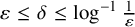
$\varepsilon \leq \delta \leq \log ^{-1}\frac 1\varepsilon $
. Let
$N>(\varepsilon +\delta )^{-c_1}$
,
$N_1\sim N^{\rho ^2}$
and
$N_2\sim N^{2\rho }$
. Then there are some
$\widetilde \Omega _N\subset \Omega $
(independent of S) satisfying
$\mathrm {meas}(\Omega \setminus \widetilde \Omega _N)\leq e^{-\frac 15 N^{\frac {3\kappa _1\rho ^2}{4}}}$
and some
$\gamma _N\in [\frac \gamma 2, \gamma ]$
so that the
$(\rho , \gamma _N, N)$
-LDE hold true for
$\boldsymbol {\omega }\in \Omega _N:=\widetilde \Omega _N\cap \mathrm {DC}_{\boldsymbol {\omega }}(N)\cap \Omega _{N_2}$
with
$\mathrm {DC}_{\boldsymbol {\omega }}(N)$
given by (2.12) and $$ \begin{align*} \widetilde\Omega_N=\bigcap_{1\leq \ell,\ell'\leq N^{4(b+d)}, \xi=\pm1, \xi'=\pm1, 0<|\boldsymbol{k}|\leq 2N^2}\widetilde\Omega_{\boldsymbol{k},\ell,\ell',\xi,\xi'}, \end{align*} $$where
$$ \begin{align*} \widetilde\Omega_{\boldsymbol{k},\ell,\ell',\xi,\xi'}:=\left\{\boldsymbol{\omega}\in\Omega:\ |\boldsymbol{k}\cdot\boldsymbol{\omega}+\xi {\lambda_\ell}-\xi'{\lambda_{\ell'}}|>10e^{-\frac 14 N^{\frac{3\kappa_1\rho^2}{4}}}\right\}, \end{align*} $$$\gamma _N\geq \gamma _{N_1}-N^{-\kappa }$
and
$\lambda _\ell = \lambda _\ell (\boldsymbol {\alpha }, \boldsymbol {\theta })$
(
${1\leq \ell \leq N^{4(b+d)}})$
are all eigenvalues of the operators
$\mathcal H_{Q}(\boldsymbol {\alpha }, \boldsymbol {\theta })$
for all
$Q\subset [-100N^2, 100N^2]^d$
satisfying $$ \begin{align*}Q\in\bigcup_{\tilde N\in [\frac14N^{\kappa_1\rho^2}, N^{\kappa_2\rho^2}]}\mathcal{ER}_{\mathbb Z^d}(\tilde N).\end{align*} $$
























Remark 2.12. Note that the sets
$\Omega _N$
 are independent of S. This will be important for later nonlinear applications. Moreover, we have
$\Omega _{N}\subset \Omega _{N-1}\subset \cdots \subset \Omega _{N_0}=\Omega $
are independent of S. This will be important for later nonlinear applications. Moreover, we have
$\Omega _{N}\subset \Omega _{N-1}\subset \cdots \subset \Omega _{N_0}=\Omega $
 and
$\Omega _N$
and
$\Omega _N$
 is a semi-algebraic set of
$\mathrm {deg}\ \Omega _N\leq N^{10(b+d)}$
is a semi-algebraic set of
$\mathrm {deg}\ \Omega _N\leq N^{10(b+d)}$
 and
$\mathrm {meas}(\Omega _{N^{2\rho }}\setminus \Omega _N)\leq e^{-\frac 12 N^{\rho ^4}}.$
and
$\mathrm {meas}(\Omega _{N^{2\rho }}\setminus \Omega _N)\leq e^{-\frac 12 N^{\rho ^4}}.$

Remark 2.13. One may observe that this LDT is for a fixed operator H; while the linearized operator is varying in a Newton scheme. This issue, however, can be remedied by using that the Green’s function estimates in LDE (at scale N) are stable under perturbations of order
$e^{-N^2}$
 using Lemma B.1. The sup-exponentially decaying error (cf. (3.14)) in the Newton scheme can ensure this. More precisely, let

We can replace H in LDT with a sequence of operators
$H^{(\ell )}(\sigma )=D{(\sigma )}+\delta S_\ell $
 (
$\ell \geq 1$
(
$\ell \geq 1$
 ) satisfying (we hide the dependence on
$\xi ,\xi '\in \{\pm \}$
) satisfying (we hide the dependence on
$\xi ,\xi '\in \{\pm \}$
 )
)

It is remarkable that in our LDT,
$\Omega _N$
 does not depend on S. So with this modification, the conclusion of LDT becomes for
$\boldsymbol {\omega }\in \Omega _N, H^{(\ell )}$
does not depend on S. So with this modification, the conclusion of LDT becomes for
$\boldsymbol {\omega }\in \Omega _N, H^{(\ell )}$
 has
$(\rho , \gamma _N', N)$
has
$(\rho , \gamma _N', N)$
 -LDE for all
$\ell \geq N\geq \log ^3{\frac {1}{\varepsilon +\delta }}$
-LDE for all
$\ell \geq N\geq \log ^3{\frac {1}{\varepsilon +\delta }}$
 (
$\Sigma _N$
(
$\Sigma _N$
 depending only on
$S_\ell $
depending only on
$S_\ell $
 ,
$1\leq \ell \leq N$
,
$1\leq \ell \leq N$
 ).
).
Indeed, assume we have established the LDE at scale
$N_1=N^{\rho ^2}$
 for all
$H^{(\ell )}$
for all
$H^{(\ell )}$
 with
$\ell \geq N_1$
with
$\ell \geq N_1$
 . Then it suffices to establish
$(\rho , \gamma _N', N)$
. Then it suffices to establish
$(\rho , \gamma _N', N)$
 -LDE for
$H^{(N)}$
-LDE for
$H^{(N)}$
 , since for all
$\ell>N$
, since for all
$\ell>N$
 ,
,

and
$(\rho , \gamma _N', N)$
 -LDE for
$H^{(\ell )}$
-LDE for
$H^{(\ell )}$
 can be obtained via the perturbation argument (cf. Lemma B.1). Next, we fix
$S_\ell \equiv S_{N_1}$
can be obtained via the perturbation argument (cf. Lemma B.1). Next, we fix
$S_\ell \equiv S_{N_1}$
 for
$\ell \in [N_1, N]$
for
$\ell \in [N_1, N]$
 . Similar to the proof of Lemma 2.20, we can show using the modified resolvent identities Lemmas B.3, B.5, B.6 (e.g., taking into account the power-law factor in the estimate of
$S_\ell $
. Similar to the proof of Lemma 2.20, we can show using the modified resolvent identities Lemmas B.3, B.5, B.6 (e.g., taking into account the power-law factor in the estimate of
$S_\ell $
 ) that
$H^{(N_1)}$
) that
$H^{(N_1)}$
 satisfies
$(\rho , \gamma _N'', N)$
satisfies
$(\rho , \gamma _N'', N)$
 -LDE with

Finally, using again the perturbation argument Lemma B.1 and

we get that
$H^{(N)}$
 satisfies
$(\rho , \gamma _N', N)$
satisfies
$(\rho , \gamma _N', N)$
 -LDE by the assumptions on
$\gamma _\ell ,\gamma _\ell '$
-LDE by the assumptions on
$\gamma _\ell ,\gamma _\ell '$
 .
.
Remark 2.14. In the large scales case, we assume
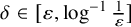
$\delta \in [\varepsilon , \log ^{-1}\frac {1}{\varepsilon }]$
 . The condition
$\delta \geq \varepsilon $
. The condition
$\delta \geq \varepsilon $
 is necessary since (2.13) as mentioned above. The restriction
$\delta \leq \log ^{-1}\frac {1}{\varepsilon }$
is necessary since (2.13) as mentioned above. The restriction
$\delta \leq \log ^{-1}\frac {1}{\varepsilon }$
 , however, is due to the fact that we need to use Bourgain’s geometric lemma in the form of Lemma 2.5 to handle the large
$\boldsymbol {|}\boldsymbol {n}|$
, however, is due to the fact that we need to use Bourgain’s geometric lemma in the form of Lemma 2.5 to handle the large
$\boldsymbol {|}\boldsymbol {n}|$
 regime estimates. In fact, if we assume that
$\mathcal W$
regime estimates. In fact, if we assume that
$\mathcal W$
 (cf. (2.11)) satisfies
$\mathrm {meas}([0,1]^{2d}\setminus \mathcal W)=o(1)$
(cf. (2.11)) satisfies
$\mathrm {meas}([0,1]^{2d}\setminus \mathcal W)=o(1)$
 (rather than the quantitative version
$\mathrm {meas}([0,1]^{2d}\setminus \mathcal W)=O(\log ^{-c}\frac {1}{\varepsilon +\delta })$
(rather than the quantitative version
$\mathrm {meas}([0,1]^{2d}\setminus \mathcal W)=O(\log ^{-c}\frac {1}{\varepsilon +\delta })$
 in the present work), we can remove the condition
$\delta \leq \log ^{-1}\frac {1}{\varepsilon }$
in the present work), we can remove the condition
$\delta \leq \log ^{-1}\frac {1}{\varepsilon }$
 (cf. Remark 2.24 for details).
This LDT will be proved in detail in the following three sections.
2.6.1 The small scales LDE
This section is devoted to the proof of LDE for small scales, that is,

In this case, we only use the standard Neumann series argument. As a result, we can establish LDE for all
$\boldsymbol {\omega }\in \Omega .$
 We have
Lemma 2.15. Let

Let
$0<\rho <\frac {1}{10^4}$
 . Then there is some
$\delta _1=\delta _1(b,d,C_2, \rho )>0$
. Then there is some
$\delta _1=\delta _1(b,d,C_2, \rho )>0$
 so that if
$0<\varepsilon +\delta \leq \delta _1,$
so that if
$0<\varepsilon +\delta \leq \delta _1,$
 for
for

we have

Moreover, if
$\sigma \notin \Sigma _N$
 , we have for all
$\Lambda \in (\boldsymbol {0},\boldsymbol {n})+\mathcal {ER}_{\boldsymbol {0}}(N)$
, we have for all
$\Lambda \in (\boldsymbol {0},\boldsymbol {n})+\mathcal {ER}_{\boldsymbol {0}}(N)$
 with
$|\boldsymbol {n}|\leq 10N$
with
$|\boldsymbol {n}|\leq 10N$
 ,
,


where

Remark 2.16. In this lemma, we make no restrictions on
$\boldsymbol {\omega }.$

Proof. We first establish the measure bound (2.15). We have

where in the last inequality we use
$0<\varepsilon +\delta \leq \delta _1^{(1)}(b,d,\rho )\ll 1$
 to ensure
$N\geq \log ^{3}\frac {1}{\varepsilon +\delta }\geq N_0(b,d,\rho )\gg 1.$
to ensure
$N\geq \log ^{3}\frac {1}{\varepsilon +\delta }\geq N_0(b,d,\rho )\gg 1.$

Next, we let
$\sigma \notin \Sigma _N$
 and fix any
$\Lambda \in (\boldsymbol {0}, \boldsymbol {n})+\mathcal {ER}_{\boldsymbol {0}}(N)$
and fix any
$\Lambda \in (\boldsymbol {0}, \boldsymbol {n})+\mathcal {ER}_{\boldsymbol {0}}(N)$
 with
$|\boldsymbol {n}|\leq 10N$
with
$|\boldsymbol {n}|\leq 10N$
 . Let
$A=D_{\Lambda }(\sigma ), B=\delta S_\Lambda $
. Let
$A=D_{\Lambda }(\sigma ), B=\delta S_\Lambda $
 . We have

Note that

assuming
$0<\varepsilon +\delta \leq \delta _1^{(2)}(b,d, C_2, \rho )\ll 1.$
 So we can apply Lemma B.1 with
$A=D_{\Lambda }(\sigma ), B=\delta S_\Lambda , \epsilon _2=C_2\delta , \epsilon _1=e^{-N^\rho }, M=0, X=\Lambda $
So we can apply Lemma B.1 with
$A=D_{\Lambda }(\sigma ), B=\delta S_\Lambda , \epsilon _2=C_2\delta , \epsilon _1=e^{-N^\rho }, M=0, X=\Lambda $
 to obtain (we hide the dependence on
$\xi , \xi '$
to obtain (we hide the dependence on
$\xi , \xi '$
 )
)

Then for
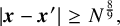
$|\boldsymbol {x}-\boldsymbol {x}'|\geq N^{\frac 89},$

which implies

Then both (2.16) and (2.17) hold true if we assume that

and
$\sigma \notin \Sigma _N.$

2.6.2 The intermediate scales LDE
This section and the next deal with intermediate-scale LDE. We will show that the LDE hold true for all
$\boldsymbol {\omega }\in \Omega $
 and scales in the range

where
$c_1$
 is given by Theorem 2.2. In this case, the analysis in Section 2.4 becomes essential.
Lemma 2.17. Let
$0<\rho <\frac {1}{10^4}$
 . There is some
$\delta _2=\delta _2(b,d, K, V, \rho , c_1, C_2)>0$
. There is some
$\delta _2=\delta _2(b,d, K, V, \rho , c_1, C_2)>0$
 so that the following holds for
$0<\varepsilon +\delta \leq \delta _2.$
so that the following holds for
$0<\varepsilon +\delta \leq \delta _2.$
 Assume
$(\boldsymbol {\alpha }, \boldsymbol {\theta })\in \mathcal {M}$
Assume
$(\boldsymbol {\alpha }, \boldsymbol {\theta })\in \mathcal {M}$
 (cf. Theorem 2.2) and fix

Then for each
$\boldsymbol {\omega }\in \Omega $
 , there exists a set
$\Sigma _N\subset \mathbb R$
, there exists a set
$\Sigma _N\subset \mathbb R$
 with
with

so that if
$\sigma \notin \Sigma _N$
 , then for all
$\Lambda \in (\boldsymbol {0}, \boldsymbol {n})+\mathcal {ER}_{\boldsymbol {0}}(N)$
, then for all
$\Lambda \in (\boldsymbol {0}, \boldsymbol {n})+\mathcal {ER}_{\boldsymbol {0}}(N)$
 with
$|\boldsymbol {n}|\leq 10N$
with
$|\boldsymbol {n}|\leq 10N$
 ,
,

where

with
$\gamma _0$
 given by (2.18) and
$\vartheta>0$
given by (2.18) and
$\vartheta>0$
 by Lemma B.3.
Remark 2.18. Note that this lemma also holds for all
$\boldsymbol {\omega }\in \Omega $
 .
.
Proof. The proof is based on the clustering property (cf. (2) of Theorem 2.2), Schur’s complement argument, Rouché’s theorem and the iteration of resolvent identities. So we first choose
$0<\varepsilon +\delta \leq c(b,d,K,V, \max \limits _{1\leq \ell \leq b}|\boldsymbol {n}_\ell |)\ll 1$
 so that Theorem 2.2 holds true. Then the proof can be decomposed into two steps.
Step 1. We define

where

We first show that

where

In fact, if
$\sigma \notin \bigcup \limits _{(\xi ,\boldsymbol {i})\in \Lambda } I_{\xi , \boldsymbol {i}},$
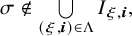 then for each
$\boldsymbol {\omega }\in \Omega ,$
then for each
$\boldsymbol {\omega }\in \Omega ,$


Since
$N\geq 10^{- \frac 1\rho } \log ^{\frac {1}{\rho }} \frac {1}{\varepsilon +\delta }$
 , the Neumann series argument implies

when
$\sigma \notin \bigcup \limits _{(\xi ,\boldsymbol {i})\in \Lambda } I_{\xi , \boldsymbol {i}}.$
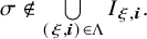 This proves (2.20) and

In the following, we estimate
$\mathrm {meas}(\Sigma _\Lambda \cap I_{\xi , \boldsymbol {i}}).$
 For this purpose, we fix any
$\xi ^*\in \{+,-\}$
For this purpose, we fix any
$\xi ^*\in \{+,-\}$
 ,
$\boldsymbol {i}^*=(\boldsymbol {k}^*, \boldsymbol {n}^*)$
,
$\boldsymbol {i}^*=(\boldsymbol {k}^*, \boldsymbol {n}^*)$
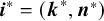 and denote

where

We will study
$G_\Lambda (\sigma )$
 for
$\sigma \in I^*.$
for
$\sigma \in I^*.$
 From (2) of Theorem 2.2, we have for every
$\sigma ^*\in \mathbb R$
From (2) of Theorem 2.2, we have for every
$\sigma ^*\in \mathbb R$
 , there exists
$B_*=B_*^+\cup B_*^-\subset \Lambda $
, there exists
$B_*=B_*^+\cup B_*^-\subset \Lambda $
 with
$\# B_*^{\pm }\leq b$
with
$\# B_*^{\pm }\leq b$
 so that

Similar to the proof of (2.20), if (we denote
$\mathbb D_r(z):=\{w\in \mathbb C:\ |w-z|\leq r\}$
 )
$z\in \mathbb {D}_{(\varepsilon +\delta )^{\frac {1}{8b}}/10}(\sigma ^*),$
)
$z\in \mathbb {D}_{(\varepsilon +\delta )^{\frac {1}{8b}}/10}(\sigma ^*),$
 then
then

So we have an analytic extension of
${H}_\Lambda (z)$
 to
$z\in \mathbb {D}_{(\varepsilon +\delta )^{\frac {1}{8b}}/10}(\sigma ^*)$
to
$z\in \mathbb {D}_{(\varepsilon +\delta )^{\frac {1}{8b}}/10}(\sigma ^*)$
 and
and

More importantly, if we denote
$\Lambda ^c=\Lambda \setminus B_*$
 , then by the Neumann series argument, we have for all
$z\in \mathbb {D}_{(\varepsilon +\delta )^{\frac {1}{8b}}/10}(\sigma ^*),$
, then by the Neumann series argument, we have for all
$z\in \mathbb {D}_{(\varepsilon +\delta )^{\frac {1}{8b}}/10}(\sigma ^*),$


In the following, we estimate
$G_{\Lambda }(z)$
 using the Schur complement reduction. We define

Obviously, we have

and

Now we consider
$\det S(z)$
 . Combining (2.22) and (2.23) yields

where
$\sigma _\ell \in \{-\boldsymbol {k}\cdot \boldsymbol {\omega }- \mu _{\boldsymbol {n}}\}_{(\boldsymbol {k}, \boldsymbol {n})\in B_*^+}\cup \{-\boldsymbol {k}\cdot \boldsymbol {\omega }+\mu _{\boldsymbol {n}}\}_{(\boldsymbol {k}, \boldsymbol {n})\in B_*^-}.$
 Recalling the definition of
$B_*$
Recalling the definition of
$B_*$
 , we must have

From (2.21), there exists at least one
$\sigma _\ell $
 so that
$|\sigma _\ell -\sigma ^*|=O((\varepsilon +\delta )^{1-c_1}).$
so that
$|\sigma _\ell -\sigma ^*|=O((\varepsilon +\delta )^{1-c_1}).$
 At this stage, we need a useful result.
Lemma 2.19. Let
$\varphi =\left (\frac {14}{15}\right )^{\frac {1}{5b}}<1$
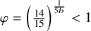 . There is
$0\leq \ell _*\leq 5b-1$
. There is
$0\leq \ell _*\leq 5b-1$
 so that

where for
$0\leq \ell \leq 5b$
 ,
,

Proof of Lemma 2.19
It suffices to note that

The proof then follows from the pigeonhole principle since
$\#B_*\leq 2b$
 .
.
Let
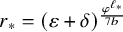
$r_*=(\varepsilon +\delta )^{\frac {\varphi ^{\ell _*}}{7b}}$
 , where
$\varphi $
, where
$\varphi $
 and
$\ell _*$
and
$\ell _*$
 are defined in Lemma 2.19. From Lemma 2.19, we can restrict our considerations on
$\mathbb {A}_*$
are defined in Lemma 2.19. From Lemma 2.19, we can restrict our considerations on
$\mathbb {A}_*$
 with
with

Then

Let

We have
$\mathcal K\neq \emptyset $
 and for
$\ell \not \in \mathcal K$
and for
$\ell \not \in \mathcal K$
 ,
,

As a result, we can write for
$z\in \mathbb {A}_*,$


It holds that

Applying Rouché’s theorem shows that the function
$\frac {\det S(z)}{\prod _{\ell \notin \mathcal K}(z-\sigma _\ell )}$
 has exactly
$\#\mathcal K$
has exactly
$\#\mathcal K$
 zeros (denoted by
$z_\ell ,\ \ell \in \mathcal K$
zeros (denoted by
$z_\ell ,\ \ell \in \mathcal K$
 ) in
$ \mathbb {D}_{20r_*}(\sigma ^*).$
) in
$ \mathbb {D}_{20r_*}(\sigma ^*).$
 From
$\sigma _\ell \in \mathbb {D}_{10r_*}(\sigma ^*)$
From
$\sigma _\ell \in \mathbb {D}_{10r_*}(\sigma ^*)$
 , we also get

From similar analysis, we can obtain that (2.24) also has exactly
$\#\mathcal {K}$
 zeros in
$\mathbb {A}_*$
zeros in
$\mathbb {A}_*$
 , which implies that
$\{z_\ell \}_{\ell \in \mathcal {K}}$
, which implies that
$\{z_\ell \}_{\ell \in \mathcal {K}}$
 are all zeros of (2.24) in
$\mathbb {A}_*$
are all zeros of (2.24) in
$\mathbb {A}_*$
 . So on
$\mathbb {A}_*$
. So on
$\mathbb {A}_*$
 , we have

where g is analytic on
$\mathbb {A}_*$
 with
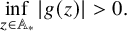
$\inf \limits _{z\in \mathbb {A}_*}|g(z)|>0.$
with
$\inf \limits _{z\in \mathbb {A}_*}|g(z)|>0.$
 Using (2.25) and (2.26), we have

Using the maximum principle then leads to

We have established on
$\mathbb {A}_*,$


In particular, one has for all
$z\in \mathbb {A}_*,$


assuming
$0<\varepsilon +\delta \leq c(b)\ll 1.$
 Thus combining Hadamard’s inequality and Cramer’s rule implies for
$z\in \mathbb {A}_*,$
Thus combining Hadamard’s inequality and Cramer’s rule implies for
$z\in \mathbb {A}_*,$


Applying the Schur complement argument shows that for
$z\in \mathbb {A}_*,$


Recall that
$I^*\subset \mathbb {A}_*$
 . So for
$\sigma \in I^*,$
. So for
$\sigma \in I^*,$
 we have

and

This implies

and subsequently

which combined with (2.19) shows

Step 2. In this step, we prove the off-diagonal exponential decay of
$G_\Lambda (\sigma )((\boldsymbol {x},\xi );(\boldsymbol {x}', \xi '))$
 assuming
$\sigma \not \in \Sigma _{N}$
assuming
$\sigma \not \in \Sigma _{N}$
 and
$\Lambda \in (\boldsymbol {0}, \boldsymbol {n})+\mathcal {ER}_{\boldsymbol {0}}(N)$
and
$\Lambda \in (\boldsymbol {0}, \boldsymbol {n})+\mathcal {ER}_{\boldsymbol {0}}(N)$
 with
$|\boldsymbol {n}|\leq 10N.$
with
$|\boldsymbol {n}|\leq 10N.$
 By Theorem 2.2, we know that there exists
$B\subset \Lambda $
By Theorem 2.2, we know that there exists
$B\subset \Lambda $
 so that

Using the Neumann series argument (cf. Lemma B.1) yields that for any
$\Lambda '\subset \Lambda $
 with
$\Lambda '\cap B=\emptyset ,$
with
$\Lambda '\cap B=\emptyset ,$


We say that
$\mathcal {ER}(\sqrt {N})\ni Q,\ Q\subset \Lambda $
 is
$\sqrt {N}$
is
$\sqrt {N}$
 -regular if both (2.27) and (2.28) hold with
$\Lambda '=Q.$
-regular if both (2.27) and (2.28) hold with
$\Lambda '=Q.$
 Otherwise, Q is called
$\sqrt {N}$
Otherwise, Q is called
$\sqrt {N}$
 -singular. Let
$\mathcal {F}$
-singular. Let
$\mathcal {F}$
 be any family of pairwise disjoint
$\sqrt {N}$
be any family of pairwise disjoint
$\sqrt {N}$
 -singular sets contained in
$\Lambda $
-singular sets contained in
$\Lambda $
 . We obtain

We have established the sublinear bound. Then applying the coupling lemma, that is, Lemma B.3 of [Reference LiuLiu22], shows

where

This proves the off-diagonal exponential decay estimates.
We have completed the proof of Lemma 2.17.
2.6.3 The large scales LDE
In this section, we will prove the LDE for

To perform the multi-scale scheme, we need two small scales
$N_1<N_2$
 with
with

We assume the LDE hold for
$\boldsymbol {\omega }\in \Omega _{N_2}\subset \Omega _{N_1}$
 .
.
Then we have
Lemma 2.20. There are some
$0<c_2=c_2(b,d)\leq \frac {1}{10^4(b+d)^2}$
 and some

so that the following holds true for
$0<\varepsilon +\delta \leq \delta _3$
 ,
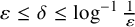
$\varepsilon \leq \delta \leq \log ^{-1}\frac {1}{\varepsilon }$
,
$\varepsilon \leq \delta \leq \log ^{-1}\frac {1}{\varepsilon }$
 and
$0<\rho \leq c_2\kappa _1$
and
$0<\rho \leq c_2\kappa _1$
 with
$\kappa _1$
with
$\kappa _1$
 given by Lemma 2.5. Let
$(\boldsymbol {\alpha }, \boldsymbol {\theta })\in \mathcal W$
given by Lemma 2.5. Let
$(\boldsymbol {\alpha }, \boldsymbol {\theta })\in \mathcal W$
 (cf. (2.11)) and N satisfy

Then there is a semi-algebraic set
$\widetilde \Omega _N\subset \Omega $
 (cf. Lemma 2.26) with
$\mathrm { meas}(\Omega \setminus \widetilde \Omega _N)\leq e^{-\frac 15N^{\frac {3\kappa _1\rho ^2}{4}}}$
(cf. Lemma 2.26) with
$\mathrm { meas}(\Omega \setminus \widetilde \Omega _N)\leq e^{-\frac 15N^{\frac {3\kappa _1\rho ^2}{4}}}$
 and
$\deg \ \widetilde \Omega _N\leq N^{5(b+d)}$
and
$\deg \ \widetilde \Omega _N\leq N^{5(b+d)}$
 so that, for
$\boldsymbol {\omega }\in \mathrm {DC}_{\boldsymbol {\omega }}(N)\cap \widetilde \Omega _N\cap {\Omega _{N_2}}$
so that, for
$\boldsymbol {\omega }\in \mathrm {DC}_{\boldsymbol {\omega }}(N)\cap \widetilde \Omega _N\cap {\Omega _{N_2}}$
 (with
$\mathrm { DC}_{\boldsymbol {\omega }}(N)$
(with
$\mathrm { DC}_{\boldsymbol {\omega }}(N)$
 given by (2.12)), there is some
$\Sigma _N\subset \mathbb R$
given by (2.12)), there is some
$\Sigma _N\subset \mathbb R$
 with
$\mathrm {meas}(\Sigma _N)\leq e^{-N^{\rho }}$
with
$\mathrm {meas}(\Sigma _N)\leq e^{-N^{\rho }}$
 , so that, if
$\sigma \notin \Sigma _N$
, so that, if
$\sigma \notin \Sigma _N$
 , then for all
$\Lambda \in (\boldsymbol {0}, \boldsymbol {n})+\mathcal {ER}_{\boldsymbol {0}}(N)$
, then for all
$\Lambda \in (\boldsymbol {0}, \boldsymbol {n})+\mathcal {ER}_{\boldsymbol {0}}(N)$
 with
$|\boldsymbol {n}|\leq 10N,$
with
$|\boldsymbol {n}|\leq 10N,$


where
$[\frac \gamma 2, \gamma ]\ni \gamma _N\geq \gamma _{N_1}-N^{-\kappa }$
 (cf. (2.35)).
We begin with a useful definition.
Definition 2.21 (
$\sigma $
-good)

For
$\Lambda \in \mathcal {ER}(L)$
 , we say
$\Lambda $
, we say
$\Lambda $
 is
$\sigma $
is
$\sigma $
 -good if

where
$\gamma _L\in [\frac \gamma 2, \gamma ]$
 , and
$\sigma $
, and
$\sigma $
 -bad, if one of the inequalities is violated.
The proof of Lemma 2.20 is based on matrix-valued Cartan’s lemma (Lemma 2.25) and iterations of resolvent identities. To apply Cartan’s lemma, one needs to establish the sublinear bound on
$\sigma $
 -bad
$\Lambda \in (\boldsymbol {k}, \boldsymbol {n})+\mathcal {ER}_{\boldsymbol {0}}(N_1)$
-bad
$\Lambda \in (\boldsymbol {k}, \boldsymbol {n})+\mathcal {ER}_{\boldsymbol {0}}(N_1)$
 contained in
$\Lambda _N$
contained in
$\Lambda _N$
 : If
$|\boldsymbol {n}|\leq 10N_1$
: If
$|\boldsymbol {n}|\leq 10N_1$
 , the sublinear bound can be obtained via the Töplitz property of H in the
$\boldsymbol {k}$
, the sublinear bound can be obtained via the Töplitz property of H in the
$\boldsymbol {k}$
 -direction together with the semi-algebraic sets theory (cf. Lemma 2.22); for
$|\boldsymbol {n}|>10N_1$
-direction together with the semi-algebraic sets theory (cf. Lemma 2.22); for
$|\boldsymbol {n}|>10N_1$
 , we will use the short-range property of S and Bourgain’s geometric lemma (Lemma 2.5) to prove the sublinear bound. Once the sublinear bound is derived, one can use the Cartan’s lemma and resolvent identities to finish the proof of large scales LDE.
We need the following ingredients to prove Lemma 2.20.
Lemma 2.22. There is some
$0<c_2=c_2(b,d)\leq \frac {1}{10^4(b+d)^2}$
 so that the following holds true. Assume that LDE hold true at scale
$N_1$
so that the following holds true. Assume that LDE hold true at scale
$N_1$
 with
with

If
$0<\rho \leq c_2$
 , then for all
$\sigma \in \mathbb R$
, then for all
$\sigma \in \mathbb R$
 , the number of
$\sigma $
, the number of
$\sigma $
 -bad
$\Lambda \in (\boldsymbol {k},\boldsymbol {n})+\mathcal {ER}_{\boldsymbol {0}}(N_1)$
-bad
$\Lambda \in (\boldsymbol {k},\boldsymbol {n})+\mathcal {ER}_{\boldsymbol {0}}(N_1)$
 satisfying
$|\boldsymbol {k}|\leq N^2$
satisfying
$|\boldsymbol {k}|\leq N^2$
 and
$|\boldsymbol {n}|\leq 10N_1$
and
$|\boldsymbol {n}|\leq 10N_1$
 is at most
$N^{\frac {1}{10^3(b+d)^2}}.$
is at most
$N^{\frac {1}{10^3(b+d)^2}}.$

Proof. First, we define
$\widetilde \Sigma _{N_1}$
 to be the set of
$\sigma \in \mathbb R$
to be the set of
$\sigma \in \mathbb R$
 so that, there is
$\Lambda \in (\boldsymbol {0}, \boldsymbol {n})+\mathcal {ER}_{\boldsymbol {0}}(N_1)$
so that, there is
$\Lambda \in (\boldsymbol {0}, \boldsymbol {n})+\mathcal {ER}_{\boldsymbol {0}}(N_1)$
 satifying
$|\boldsymbol {n}|\leq 10N_1$
satifying
$|\boldsymbol {n}|\leq 10N_1$
 , which is
$\sigma $
, which is
$\sigma $
 -bad. We then obtain using LDE at scale
$N_1,$
-bad. We then obtain using LDE at scale
$N_1,$


for
$N_1\geq N_0(b,d,\rho ).$
 Using the Hilbert-Schmidt norm and Cramer’s rule, we can identify
$\widetilde \Sigma _{N_1}$
Using the Hilbert-Schmidt norm and Cramer’s rule, we can identify
$\widetilde \Sigma _{N_1}$
 with a semi-algebraic set of
$\deg \widetilde \Sigma _{N_1}\leq N_1^{C(b,d)}$
with a semi-algebraic set of
$\deg \widetilde \Sigma _{N_1}\leq N_1^{C(b,d)}$
 . Then using Basu-Pollack-Roy Theorem [Reference Basu, Pollack and RoyBPR96] on Betti numbers of a semi-algebraic set (cf. also Proposition 9.2 of [Reference BourgainBou05a]), we have a decomposition of

where each
$I_\ell $
 is an interval of length
$|I_\ell |\leq e^{-\frac 12 N_1^{\rho }}.$
is an interval of length
$|I_\ell |\leq e^{-\frac 12 N_1^{\rho }}.$
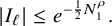 Now assume that
$\Lambda \in (\boldsymbol {k},\boldsymbol {n})+\mathcal {ER}_{\boldsymbol {0}}(N_1)$
Now assume that
$\Lambda \in (\boldsymbol {k},\boldsymbol {n})+\mathcal {ER}_{\boldsymbol {0}}(N_1)$
 and
$\Lambda '\in (\boldsymbol {k}',\boldsymbol {n})+\mathcal {ER}_{\boldsymbol {0}}(N_1)$
and
$\Lambda '\in (\boldsymbol {k}',\boldsymbol {n})+\mathcal {ER}_{\boldsymbol {0}}(N_1)$
 , which are all
$\sigma $
, which are all
$\sigma $
 -bad for some
$|\boldsymbol {n}|\leq 10N_1, \boldsymbol {k}\neq \boldsymbol {k}'$
-bad for some
$|\boldsymbol {n}|\leq 10N_1, \boldsymbol {k}\neq \boldsymbol {k}'$
 and
$|\boldsymbol {k}|, |\boldsymbol {k}'|\leq N^2$
and
$|\boldsymbol {k}|, |\boldsymbol {k}'|\leq N^2$
 . Then from the Töplitz property of
${H}(\sigma )$
. Then from the Töplitz property of
${H}(\sigma )$
 in the
$\boldsymbol {k}$
in the
$\boldsymbol {k}$
 -direction, we obtain

As a result, by
$\boldsymbol {k}\neq \boldsymbol {k}'$
 with
$|\boldsymbol {k}|, |\boldsymbol {k}'|\leq N^2$
with
$|\boldsymbol {k}|, |\boldsymbol {k}'|\leq N^2$
 ,
$\boldsymbol {\omega }\in \mathrm {DC}_{\boldsymbol {\omega }}(N)$
,
$\boldsymbol {\omega }\in \mathrm {DC}_{\boldsymbol {\omega }}(N)$
 (cf. (2.12)) and
$N\sim N_1^{\frac {1}{\rho ^2}}$
(cf. (2.12)) and
$N\sim N_1^{\frac {1}{\rho ^2}}$
 , we have for
$N_1\geq N_0(b,d, \rho , K,V),$
, we have for
$N_1\geq N_0(b,d, \rho , K,V),$


which implies
$\boldsymbol {k}$
 and
$\boldsymbol {k}'$
and
$\boldsymbol {k}'$
 cannot stay in the same interval
$I_\ell $
cannot stay in the same interval
$I_\ell $
 for
$1\leq \ell \leq N_1^{C(b,d)}.$
for
$1\leq \ell \leq N_1^{C(b,d)}.$
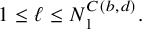 Thus we have shown that the number of
$\sigma $
Thus we have shown that the number of
$\sigma $
 -bad
$\Lambda \in (\boldsymbol {k},\boldsymbol {n})+\mathcal {ER}_{\boldsymbol {0}}(N_1)$
-bad
$\Lambda \in (\boldsymbol {k},\boldsymbol {n})+\mathcal {ER}_{\boldsymbol {0}}(N_1)$
 with
$|\boldsymbol {n}|\leq 10N_1$
with
$|\boldsymbol {n}|\leq 10N_1$
 and
$|\boldsymbol {k}|\leq N^2$
and
$|\boldsymbol {k}|\leq N^2$
 is at most

assuming
$0<\rho \leq c_2(b,d)\leq \frac {1}{10^4(b+d)^2}. $
 This proves Lemma 2.22.
Next, we will deal with
$|\boldsymbol {n}|>10N_1$
 by combining the short-range property of S and Bourgain’s geometric lemma (cf. Lemma 2.5). For
$\Lambda \subset \mathbb Z^{b+d}$
by combining the short-range property of S and Bourgain’s geometric lemma (cf. Lemma 2.5). For
$\Lambda \subset \mathbb Z^{b+d}$
 , denote by
$\Pi _b\Lambda $
, denote by
$\Pi _b\Lambda $
 (resp.
$\Pi _d\Lambda $
(resp.
$\Pi _d\Lambda $
 ) the projection of
$\Lambda $
) the projection of
$\Lambda $
 on
$\mathbb Z^b$
on
$\mathbb Z^b$
 (resp.
$\mathbb Z^d$
(resp.
$\mathbb Z^d$
 ). For each
$\boldsymbol {k}\in \Pi _b\Lambda , $
). For each
$\boldsymbol {k}\in \Pi _b\Lambda , $
 define

We have
Lemma 2.23. Assume that
$(\boldsymbol {\alpha }, \boldsymbol {\theta })\in \mathcal {\mathcal W'}$
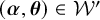 (cf. Lemma 2.5) and
$L\geq 10^{-\frac {32}{\kappa _1^2}}\log ^{\frac {4}{\kappa _1}}(\log \frac 1\varepsilon )$
(cf. Lemma 2.5) and
$L\geq 10^{-\frac {32}{\kappa _1^2}}\log ^{\frac {4}{\kappa _1}}(\log \frac 1\varepsilon )$
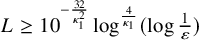 . We have
-
(1) Fix $\Lambda \in (\boldsymbol {k}', \boldsymbol {n}')+\mathcal {ER}_{\boldsymbol {0}}(L) $
with
$|\boldsymbol {n}'|>10L$
. There is a collection of
$\{\lambda _\ell =\lambda _\ell (\boldsymbol {\alpha }, \boldsymbol {\theta })\}_{1\leq \ell \leq L^{b+2d}}$
depending only on
$\Lambda , \boldsymbol {\alpha }, \boldsymbol {\theta }, V$
so that, if $$ \begin{align*}\min_{\boldsymbol{k}\in\Pi_b\Lambda, 1\leq \ell\leq L^{b+2d}, \xi=\pm1}|\sigma+\boldsymbol{k}\cdot\boldsymbol{\omega}+\xi{\lambda_\ell}|> e^{-\frac14 L^{\frac{3\kappa_1}{4}}},\end{align*} $$then $\Lambda $
is
$\sigma $
-good with
$\gamma _L=\gamma $
, where
$\kappa _1$
is given in Lemma 2.5.
-
(2) Let $L\leq N\leq e^{\log ^2 L}$
. There exists some
$\tilde \Sigma _{L}\subset \mathbb R$
with
$\mathrm { meas}(\tilde \Sigma _{L})\leq e^{-\frac 15 L^{\frac {3\kappa _1}{4}}}$
so that, if
$\sigma \notin \tilde \Sigma _{L}$
, then each
$\Lambda \in (\boldsymbol {k}, \boldsymbol {n})+\mathcal {ER}_{\boldsymbol {0}}(L) $
satisfying
$|(\boldsymbol {k},\boldsymbol {n})|\leq 100N^2$
and
$|\boldsymbol {n}|>10L$
is
$\sigma $
-good with
$\gamma _L=\gamma $
.







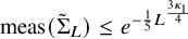





Proof. (1) Let
$\boldsymbol {k}\in \Pi _b\Lambda $
 . It is important that either
$\Lambda ({\boldsymbol {k}})\in \mathcal {ER}_{\mathbb Z^d}(L),$
. It is important that either
$\Lambda ({\boldsymbol {k}})\in \mathcal {ER}_{\mathbb Z^d}(L),$
 or
$\Lambda ({\boldsymbol {k}})$
or
$\Lambda ({\boldsymbol {k}})$
 is a rectangle of width at least L (cf. Lemma B.8). In each of the two cases, we have
$\Lambda ({\boldsymbol {k}})\in \mathcal E_{2L}^{L}$
is a rectangle of width at least L (cf. Lemma B.8). In each of the two cases, we have
$\Lambda ({\boldsymbol {k}})\in \mathcal E_{2L}^{L}$
 .
.
For
$Q\subset \Lambda ({\boldsymbol {k}}), $
 write
write

where
$\mathcal {L}_{Q}(\boldsymbol {\theta }):=\mathcal H_Q(\boldsymbol {\alpha }, \boldsymbol {\theta })$
 is defined in Lemma 2.5. Then the set of all eigenvalues of
$A_{\boldsymbol {k}, Q}$
is defined in Lemma 2.5. Then the set of all eigenvalues of
$A_{\boldsymbol {k}, Q}$
 is given by

where
$\{\lambda _\ell :=\lambda _{\ell , Q}(\boldsymbol {\alpha }, \boldsymbol {\theta })\}_{\ell =1}^{\#Q}$
 denotes the spectrum of
$\mathcal {L}_{Q}(\boldsymbol {\theta }).$
denotes the spectrum of
$\mathcal {L}_{Q}(\boldsymbol {\theta }).$
 So we have

We now can use Lemma 2.5 and resolvent identities. Since
$\boldsymbol {\alpha }\in \mathcal {A}\subset \mathcal {A}_{L}$
 , applying (1) of Lemma 2.5 with
$E_{\boldsymbol {k}}=\sigma +\boldsymbol {k}\cdot \boldsymbol {\omega }$
, applying (1) of Lemma 2.5 with
$E_{\boldsymbol {k}}=\sigma +\boldsymbol {k}\cdot \boldsymbol {\omega }$
 similar to [Reference Jitomirskaya, Liu and ShiJLS20] (cf. pages 471–472, the proof of Theorem 3.7) gives the following: For each
$\boldsymbol {m}\in \Lambda (\boldsymbol {k})$
similar to [Reference Jitomirskaya, Liu and ShiJLS20] (cf. pages 471–472, the proof of Theorem 3.7) gives the following: For each
$\boldsymbol {m}\in \Lambda (\boldsymbol {k})$
 , there exist
$\frac {1}{4}L^{\kappa _1}\leq \tilde {L} \leq L^{\kappa _2}$
, there exist
$\frac {1}{4}L^{\kappa _1}\leq \tilde {L} \leq L^{\kappa _2}$
 ,
$Q_{\boldsymbol {m}} \in \mathcal {ER}_{\mathbb Z^d}(\tilde L)$
,
$Q_{\boldsymbol {m}} \in \mathcal {ER}_{\mathbb Z^d}(\tilde L)$
 and
$\tilde {Q}_{\boldsymbol {m}}$
and
$\tilde {Q}_{\boldsymbol {m}}$
 , such that

Also for any
$ \boldsymbol {n}\in Q_{\boldsymbol {m}}\setminus \tilde {Q}_{\boldsymbol {m}}$
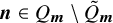 , there exist
$L_1\sim (\log L)^{\frac {4}{\kappa _1}}$
, there exist
$L_1\sim (\log L)^{\frac {4}{\kappa _1}}$
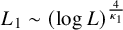 and some
$\mathcal {ER}_{\mathbb Z^d}(L_1)\ni W \subset Q_{\boldsymbol {m}}\setminus \tilde {Q}_{\boldsymbol {m}}$
and some
$\mathcal {ER}_{\mathbb Z^d}(L_1)\ni W \subset Q_{\boldsymbol {m}}\setminus \tilde {Q}_{\boldsymbol {m}}$
 such that

and

Next, assume that (set
$Q=Q_{\boldsymbol {m}}$
 )
)

Then applying Lemma B.6 of [Reference Jitomirskaya, Liu and ShiJLS20] yields for

the following estimates

Note that

where

By taking into account all
$\boldsymbol {k}\in \Pi _b\Lambda ,$
 we obtain that if

then

Note that the total number of
$\lambda _\ell $
 in (2.29) is at most

Finally, since
$|\boldsymbol {n}|>10L$
 , we know that S has the decay estimate

Then using the perturbation Lemma B.1 implies that
$\Lambda $
 is
$\sigma $
is
$\sigma $
 -good assuming (2.29) holds true. In fact, we can apply Lemma B.1 (we hide the dependence on
$\xi , \xi '$
-good assuming (2.29) holds true. In fact, we can apply Lemma B.1 (we hide the dependence on
$\xi , \xi '$
 ) with
$B=\delta S_\Lambda (\boldsymbol {x}, \boldsymbol {x}')$
) with
$B=\delta S_\Lambda (\boldsymbol {x}, \boldsymbol {x}')$
 ,
$A^{-1}(\boldsymbol {x}, \boldsymbol {x}')=\tilde G_{\Lambda }(\boldsymbol {x}, \boldsymbol {x}')$
,
$A^{-1}(\boldsymbol {x}, \boldsymbol {x}')=\tilde G_{\Lambda }(\boldsymbol {x}, \boldsymbol {x}')$
 and
$c=2\gamma , \epsilon _1=e^{-\frac 12 L^{\frac 34}}, M=L^{\frac 89}, \epsilon _2=C\delta e^{-6\gamma L}$
and
$c=2\gamma , \epsilon _1=e^{-\frac 12 L^{\frac 34}}, M=L^{\frac 89}, \epsilon _2=C\delta e^{-6\gamma L}$
 . Since
$\gamma \in (\frac 12, 10)$
. Since
$\gamma \in (\frac 12, 10)$
 , we obtain for
$L\geq N_0(b,d, C_2)\gg~1,$
, we obtain for
$L\geq N_0(b,d, C_2)\gg~1,$


This verifies all assumptions of Lemma B.1. So using Lemma B.1, we get

and for
$|\boldsymbol {x}-\boldsymbol {x}'|\geq L^{\frac {8}{9}}$
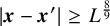 (since
$\frac 14 |\log \varepsilon |>2\gamma >1$
(since
$\frac 14 |\log \varepsilon |>2\gamma >1$
 ),
),

This proves (1) of Lemma 2.23.
Remark 2.24.
-
○ Let $L\leq N\leq e^{(\log L)^2}$
. We would also like to remark that if we take into account all these
$\Lambda \in (\boldsymbol {k}, \boldsymbol {n})+\mathcal {ER}_{\boldsymbol {0}}(L)$
with
$|(\boldsymbol {k}, \boldsymbol {n})|\leq 100N^2$
and
$|\boldsymbol {n}|>10L$
(the total number of these
$\Lambda $
is at most
$C(b,d)N^{2(b+d)}$
), then we get a sequence of real numbers
$\{{\lambda _\ell (\boldsymbol {\alpha }, \boldsymbol {\theta })}\}_{1\leq \ell \leq N^{4(b+d)}}$
. As a result, there is a set
$\tilde \Sigma _{L}\subset \mathbb R$
satisfying $$ \begin{align*}\mathrm{ meas}(\tilde\Sigma_{L})\leq e^{C(b,d)\log^2 L}e^{-\frac14 L^{\frac{3}{4}\kappa_1}}\leq e^{-\frac15 L^{\frac{3}{4}\kappa_1}}\end{align*} $$so that, for $\sigma \not \in \tilde \Sigma _{L}$
, all
$\Lambda \in (\boldsymbol {k}, \boldsymbol {n})+\mathcal {ER}_{\boldsymbol {0}}(L)$
satisfying
$|(\boldsymbol {k}, \boldsymbol {n})|\leq 100N^2$
and
$|\boldsymbol {n}|>10L$
are
$\sigma $
-good.
-
○ In the application, we typically choose $L=N_1\geq 10^{-\frac {32}{\kappa _1^2}}\log ^{\frac {4}{\kappa _1}}(\log \frac 1\varepsilon )$
. It then follows from
$ N_1\sim N^{\rho ^2}\geq (\varepsilon +\delta )^{-c_1\rho ^2}$
that a restriction like
$\delta \leq \log ^{-1}\frac 1\varepsilon $
is needed.
















(2) The conclusion is just that in Remark 2.24.
This completes the proof of Lemma 2.23.
By combining Lemma 2.22 and Lemma 2.23, we are ready to prove LDE at the scale N (indeed all scales in
$[N, N^2]$
 ). We first recall an important lemma.
Lemma 2.25 (Matrix-valued Cartan’s lemma, cf. Proposition 14.1 in [Reference BourgainBou05a])
Let
$T(\sigma )$
 be a self-adjoint
$N\times N$
be a self-adjoint
$N\times N$
 matrix-valued function of a parameter
$\sigma \in [-\beta , \beta ]$
matrix-valued function of a parameter
$\sigma \in [-\beta , \beta ]$
 satisfying the following conditions:
-
(i) $T(\sigma )$
is real analytic in
$\sigma $
and has a holomorphic extension to $$ \begin{align*} \mathbb{D}=\left\{z\in\mathbb{C}: \ |\Re z|\leq \beta,\ |\Im z|\leq \beta_1\right\} \end{align*} $$satisfying $\sup \limits _{z\in \mathbb {D}}\|T(z)\|\leq K_1,\ K_1\geq 1.$
-
(ii) For each $\sigma \in [-\beta , \beta ]$
, there is a subset
$Y\subset [1,N]$
with
$\#Y\leq M$
such that $$ \begin{align*} \|(R_{[1,N]\setminus Y}T(\sigma)R_{[1,N]\setminus Y})^{-1}\|\leq K_2, \ K_2\geq 1. \end{align*} $$
-
(iii) Assume
$$ \begin{align*} \mathrm{meas}\ \left(\{\sigma\in[-{\beta}, {\beta}]: \ \|T^{-1}(\sigma)\|\geq K_3\}\right)\leq 10^{-3}\beta_1(1+K_1)^{-1}(1+K_2)^{-1}. \end{align*} $$





Let
$0<\epsilon \leq (1+K_1+K_2)^{-10 M}.$
 Then we have

where
$C, c>0$
 are some absolute constants.
Now, we can prove Lemma 2.20.
Proof of Lemma 2.20
Recalling

we assume that for
$L=N_1, N_2$
 and
$\Lambda \in (\boldsymbol {0}, \boldsymbol {n})+\mathcal {ER}_{\boldsymbol {0}}(L)$
and
$\Lambda \in (\boldsymbol {0}, \boldsymbol {n})+\mathcal {ER}_{\boldsymbol {0}}(L)$
 with
$|\boldsymbol {n}|\leq 10L$
with
$|\boldsymbol {n}|\leq 10L$
 ,
$G_{\Lambda }(\sigma )$
,
$G_{\Lambda }(\sigma )$
 satisfies the LDE.
Without loss of generality, we only establish LDE for the Green’s function on
$\Lambda _{\mathrm {pm}, N}=\{(\boldsymbol {x}, \xi )\in \mathbb Z_{\mathrm {pm}, *}^{b+d}:\ |\boldsymbol {x}|\leq N \}= (\Lambda _{N}\times \{+, -\})\cap \mathbb Z_{\mathrm {pm}, *}^{b+d}$
 , the other cases (i.e.,
$\Lambda \in (\boldsymbol {0}, \boldsymbol {n})+{\mathcal {ER}_{\boldsymbol {0}}(N_3)}$
, the other cases (i.e.,
$\Lambda \in (\boldsymbol {0}, \boldsymbol {n})+{\mathcal {ER}_{\boldsymbol {0}}(N_3)}$
 for
$|\boldsymbol {n}|\leq 10N_3, N_3\in [N, N^2]$
for
$|\boldsymbol {n}|\leq 10N_3, N_3\in [N, N^2]$
 ) can be dealt with similarly. We define three intermediate scales between
$[N_2, N]$
) can be dealt with similarly. We define three intermediate scales between
$[N_2, N]$
 :
:

Note that from
$0<\rho \leq c_2(b,d)\leq {\frac {1}{10^4(b+d)^2}}$
 (cf. Lemma 2.22), we have

We first cover the
$\Lambda _{\mathrm {pm}, N}$
 with two overlapped subregions,
$\Lambda _{\mathrm {pm}, N}=\mathcal {R}_1\cup \mathcal {R}_2$
with two overlapped subregions,
$\Lambda _{\mathrm {pm}, N}=\mathcal {R}_1\cup \mathcal {R}_2$
 satisfying

We will apply matrix-valued Cartan’s lemma (cf. Lemma 2.25) and Bourgain’s geometric lemma [Reference BourgainBou07] (cf. Lemma 2.5) to obtain the sub-exponential growth estimates on Green’s functions. Then we apply the coupling lemmas of [Reference Bourgain, Goldstein and SchlagBGS02, Reference Jitomirskaya, Liu and ShiJLS20, Reference LiuLiu22] (cf., e.g., Lemmas B.3, B.5, B.6) based on the iteration of resolvent identities to prove the off-diagonal exponential decay of
$G_{\Lambda _{\mathrm {pm}, N}}(\sigma )$
 if desired
$\sigma $
if desired
$\sigma $
 are removed.
Before we enter the details, let us first explain why we need to divide
$\Lambda _{\mathrm {pm}, N}$
 into the above two regions. This is quite different from that in [Reference Shi and WangSW23]. Based on Lemma 2.23, we can impose the so-called weak second Melnikov’s condition on
$\boldsymbol {\omega }$
into the above two regions. This is quite different from that in [Reference Shi and WangSW23]. Based on Lemma 2.23, we can impose the so-called weak second Melnikov’s condition on
$\boldsymbol {\omega }$
 so that all
$\sigma $
so that all
$\sigma $
 -bad (cf. Definition 2.21)
$\Lambda \in (\boldsymbol {k}, \boldsymbol {n})+\mathcal {ER}_{\boldsymbol {0}}(N_1)\subset \Lambda _{\mathrm {pm}, N}$
-bad (cf. Definition 2.21)
$\Lambda \in (\boldsymbol {k}, \boldsymbol {n})+\mathcal {ER}_{\boldsymbol {0}}(N_1)\subset \Lambda _{\mathrm {pm}, N}$
 can stay only in a narrow strip region (cf. Figure 1), namely, there is some
$\boldsymbol {k}_*\in [-N, N]^b$
can stay only in a narrow strip region (cf. Figure 1), namely, there is some
$\boldsymbol {k}_*\in [-N, N]^b$
 so that

This gives the desired control on
$\sigma $
 -bad
$\Lambda $
-bad
$\Lambda $
 in the
$\boldsymbol {k}$
in the
$\boldsymbol {k}$
 -direction. To establish the sublinear bound, it remains to handle the
$\boldsymbol {n}$
-direction. To establish the sublinear bound, it remains to handle the
$\boldsymbol {n}$
 -direction. In [Reference Shi and WangSW23], the
$\boldsymbol {n}$
-direction. In [Reference Shi and WangSW23], the
$\boldsymbol {n}$
 -direction estimates can be obtained directly using the fact that
$\theta \in \mathbb R$
-direction estimates can be obtained directly using the fact that
$\theta \in \mathbb R$
 , Diophantine
$\boldsymbol {\omega }$
, Diophantine
$\boldsymbol {\omega }$
 and LDT for the corresponding quasi-periodic Schrödinger operators. Such arguments inevitably fail for
$\boldsymbol {\theta }\in \mathbb R^d$
and LDT for the corresponding quasi-periodic Schrödinger operators. Such arguments inevitably fail for
$\boldsymbol {\theta }\in \mathbb R^d$
 : There is simply no one-dimensional interval decomposition of d-dimensional semi-algebraic sets, and more essentially, the Diophantine property of
$\boldsymbol {\omega }$
: There is simply no one-dimensional interval decomposition of d-dimensional semi-algebraic sets, and more essentially, the Diophantine property of
$\boldsymbol {\omega }$
 cannot ensure the sublinear estimate in the
$\boldsymbol {n}$
cannot ensure the sublinear estimate in the
$\boldsymbol {n}$
 -direction. This motivates us to restrict
$|\boldsymbol {n}|\leq L_2$
-direction. This motivates us to restrict
$|\boldsymbol {n}|\leq L_2$
 (i.e., the region
$\mathcal {R}_1$
(i.e., the region
$\mathcal {R}_1$
 ). We can use the Cartan’s lemma and resolvent identities to deal with
$\mathcal {R}_1$
). We can use the Cartan’s lemma and resolvent identities to deal with
$\mathcal {R}_1$
 . For
$\mathcal {R}_2$
. For
$\mathcal {R}_2$
 , we take advantage of Bourgain’s geometric lemma and the short-range property of H using Lemma 2.23. Finally, it suffices to cover
$\Lambda _{\mathrm {pm}, N}$
, we take advantage of Bourgain’s geometric lemma and the short-range property of H using Lemma 2.23. Finally, it suffices to cover
$\Lambda _{\mathrm {pm}, N}$
 with four types of regions of sizes
$N_1, L_1^{\frac {9}{10}}, L_1, L_3$
with four types of regions of sizes
$N_1, L_1^{\frac {9}{10}}, L_1, L_3$
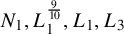 (will be specified below) contained in
$\mathcal {R}_1$
(will be specified below) contained in
$\mathcal {R}_1$
 ,
$\mathcal {R}_2$
,
$\mathcal {R}_2$
 , and apply the resolvent identities again. See Figure 1.
We first deal with
$\mathcal R_2$
 , and then
$\mathcal R_1$
, and then
$\mathcal R_1$
 .
.
Analysis in
$\mathcal {R}_2$

In this region, we can apply directly the conclusion of Lemma 2.23. In this case, we make no restriction on
$\boldsymbol {\omega }.$
 We let

For any
$\Lambda \subset \mathcal R_2$
 satisfying
$\Lambda =(\boldsymbol {k}, \boldsymbol {n})+\mathcal {ER}(L_0)$
satisfying
$\Lambda =(\boldsymbol {k}, \boldsymbol {n})+\mathcal {ER}(L_0)$
 , we have
$|\boldsymbol {n}|>L_1>10L_0$
, we have
$|\boldsymbol {n}|>L_1>10L_0$
 . Then applying Lemma 2.23 with
$L=L_0$
. Then applying Lemma 2.23 with
$L=L_0$
 and since
$0<\rho <c_2(b,d)\kappa _1\leq \frac {\kappa _1}{10^4(b+d)^2},$
and since
$0<\rho <c_2(b,d)\kappa _1\leq \frac {\kappa _1}{10^4(b+d)^2},$
 we get a set
$\tilde \Sigma _{N, 1}\subset \mathbb R$
we get a set
$\tilde \Sigma _{N, 1}\subset \mathbb R$
 satisfying

so that, if
$\sigma \notin \tilde \Sigma _{N,1}$
 , all
$\Lambda \in \mathcal {ER}(L_0)$
, all
$\Lambda \in \mathcal {ER}(L_0)$
 contained in
$ \mathcal R_2$
contained in
$ \mathcal R_2$
 are
$\sigma $
are
$\sigma $
 -good (cf. Definition 2.21).
We remark that in this case, we do not use Cartan’s lemma.
Analysis in
$\mathbf {\mathcal {R}_1}$

In this region, we need to make further restriction on
$\boldsymbol {\omega }$
 called the weak second Melnikov’s condition. More precisely, we have
Lemma 2.26. There is a sequence of real numbers
$\{\lambda _{\ell }=\lambda _\ell (\boldsymbol {\alpha }, \boldsymbol {\theta })\}_{1\leq \ell \leq N^{4(b+d)}}$
 depending only on
$V, \boldsymbol {\alpha }, \boldsymbol {\theta }$
depending only on
$V, \boldsymbol {\alpha }, \boldsymbol {\theta }$
 so that the following holds true. If
$\boldsymbol {\omega }\in \widetilde \Omega _{N}$
so that the following holds true. If
$\boldsymbol {\omega }\in \widetilde \Omega _{N}$
 with
with

then for any
$\sigma \in \mathbb R,$
 there is some
$\boldsymbol {k}_*\in [-N^2, N^2]^b$
there is some
$\boldsymbol {k}_*\in [-N^2, N^2]^b$
 so that, all
$\sigma $
so that, all
$\sigma $
 -bad
$\Lambda \in (\boldsymbol {k}, \boldsymbol {n})+\mathcal {ER}_{\boldsymbol {0}}(N_1)$
-bad
$\Lambda \in (\boldsymbol {k}, \boldsymbol {n})+\mathcal {ER}_{\boldsymbol {0}}(N_1)$
 satisfying
$|\boldsymbol {k}|\leq N^2$
satisfying
$|\boldsymbol {k}|\leq N^2$
 and
$10N_1\leq |\boldsymbol {n}|\leq 100N^2$
and
$10N_1\leq |\boldsymbol {n}|\leq 100N^2$
 must obey

In particular, we have

Remark 2.27. Indeed, in this lemma,
$\lambda _\ell (\boldsymbol {\alpha }, \boldsymbol {\theta })$
 (
${1\leq \ell \leq N^{4(b+d)}})$
(
${1\leq \ell \leq N^{4(b+d)}})$
 are eigenvalues of the operator
$\mathcal H_{Q}(\boldsymbol {\alpha }, \boldsymbol {\theta })$
are eigenvalues of the operator
$\mathcal H_{Q}(\boldsymbol {\alpha }, \boldsymbol {\theta })$
 for all
$Q\subset [-100N^2, 100N^2]^d$
for all
$Q\subset [-100N^2, 100N^2]^d$
 satisfying
$Q\in \mathcal {ER}_{\mathbb Z^d}(\tilde N_1)$
satisfying
$Q\in \mathcal {ER}_{\mathbb Z^d}(\tilde N_1)$
 for some
$\tilde N_1\in [\frac 14N_1^{\kappa _1}, N_1^{\kappa _2}]$
for some
$\tilde N_1\in [\frac 14N_1^{\kappa _1}, N_1^{\kappa _2}]$
 .
.
Proof of Lemma 2.26
The proof follows from Lemma 2.23. Applying (1) of Lemma 2.23 (cf. also Remark 2.24) with
$L=N_1$
 and taking into account of all
$\Lambda \in (\boldsymbol {k}, \boldsymbol {n})+\mathcal {ER}_{\boldsymbol {0}}(N_1)$
and taking into account of all
$\Lambda \in (\boldsymbol {k}, \boldsymbol {n})+\mathcal {ER}_{\boldsymbol {0}}(N_1)$
 with
$|(\boldsymbol {k},\boldsymbol {n})|\leq 100N^2$
with
$|(\boldsymbol {k},\boldsymbol {n})|\leq 100N^2$
 and
$|\boldsymbol {n}|>10N_1$
and
$|\boldsymbol {n}|>10N_1$
 yield a sequence
$\{{\lambda _\ell }\}_{\leq \ell \leq N^{4(b+d)}}\subset \mathbb R$
yield a sequence
$\{{\lambda _\ell }\}_{\leq \ell \leq N^{4(b+d)}}\subset \mathbb R$
 and each
$\lambda _\ell $
and each
$\lambda _\ell $
 depending only on
$\boldsymbol {\alpha }, \boldsymbol {\theta }$
depending only on
$\boldsymbol {\alpha }, \boldsymbol {\theta }$
 (but not on
$\sigma ,\boldsymbol {\omega }$
(but not on
$\sigma ,\boldsymbol {\omega }$
 ), so that if
$\Lambda =(\boldsymbol {k}, \boldsymbol {n})+\mathcal {ER}_{\boldsymbol {0}}(N_1)$
), so that if
$\Lambda =(\boldsymbol {k}, \boldsymbol {n})+\mathcal {ER}_{\boldsymbol {0}}(N_1)$
 satisfies
$|(\boldsymbol {k}, \boldsymbol {n})|\leq 100N^2$
satisfies
$|(\boldsymbol {k}, \boldsymbol {n})|\leq 100N^2$
 ,
$|\boldsymbol {n}|>10N_1$
,
$|\boldsymbol {n}|>10N_1$
 and
and

then
$\Lambda $
 is
$\sigma $
is
$\sigma $
 -good. So recalling (2.32), we have

which implies (2.34).
In the following, we assume
$\boldsymbol {\omega }\in \widetilde \Omega _N.$

Suppose now
$\Lambda '$
 with
$\Lambda '\in (\boldsymbol {k}', \boldsymbol {n}')+\mathcal {ER}_{\boldsymbol {0}}(N_1)$
with
$\Lambda '\in (\boldsymbol {k}', \boldsymbol {n}')+\mathcal {ER}_{\boldsymbol {0}}(N_1)$
 satisfying
$|\boldsymbol {k}'|\leq N^2$
satisfying
$|\boldsymbol {k}'|\leq N^2$
 and
$10N_1<|\boldsymbol {n}'|\leq 100N^2$
and
$10N_1<|\boldsymbol {n}'|\leq 100N^2$
 is
$\sigma $
is
$\sigma $
 -bad. Then there are some
$\boldsymbol {k}_*\in \Pi _b\Lambda '\subset [-N^2, N^2]^b$
-bad. Then there are some
$\boldsymbol {k}_*\in \Pi _b\Lambda '\subset [-N^2, N^2]^b$
 ,
$\xi _*=\pm 1$
,
$\xi _*=\pm 1$
 and some
$\ell _*\in [1, N^{4(b+d)}]$
and some
$\ell _*\in [1, N^{4(b+d)}]$
 so that

Now let
$\Lambda ''$
 (satisfying
$\Lambda ''\in (\boldsymbol {k}'', \boldsymbol {n}'')+\mathcal {ER}_{\boldsymbol {0}}(N_1)$
(satisfying
$\Lambda ''\in (\boldsymbol {k}'', \boldsymbol {n}'')+\mathcal {ER}_{\boldsymbol {0}}(N_1)$
 with
$|\boldsymbol {k}''|\leq N^2$
with
$|\boldsymbol {k}''|\leq N^2$
 and
$10N_1<|\boldsymbol {n}''|\leq 100N^2$
and
$10N_1<|\boldsymbol {n}''|\leq 100N^2$
 ) be another
$\sigma $
) be another
$\sigma $
 -bad region. From
$\boldsymbol {\omega }\in \widetilde \Omega _N,$
-bad region. From
$\boldsymbol {\omega }\in \widetilde \Omega _N,$
 we must have

Otherwise, there must be some
$\boldsymbol {k}'''\in \Pi _b\Lambda '', \xi '\in \{\pm 1\}, \ell '$
 so that,
$\boldsymbol {k}_*\neq \boldsymbol {k}'''$
so that,
$\boldsymbol {k}_*\neq \boldsymbol {k}'''$
 and
and

which contradicts
$\boldsymbol {\omega }\in \widetilde \Omega _N$
 . We have established that all
$\sigma $
. We have established that all
$\sigma $
 -bad elementary
$N_1$
-bad elementary
$N_1$
 -regions
$\Lambda $
-regions
$\Lambda $
 with centers
$(\boldsymbol {k}, \boldsymbol {n})$
with centers
$(\boldsymbol {k}, \boldsymbol {n})$
 satisfying
$|\boldsymbol {k}|\leq N^2$
satisfying
$|\boldsymbol {k}|\leq N^2$
 and
$10N_1<|\boldsymbol {n}|\leq 100N^2$
and
$10N_1<|\boldsymbol {n}|\leq 100N^2$
 must satisfy (2.33).
In the following, we always assume
$\boldsymbol {\omega }\in \widetilde \Omega _N$
 . Under this condition, we first give a geometric construction of the a region
$\Lambda ^\dagger $
. Under this condition, we first give a geometric construction of the a region
$\Lambda ^\dagger $
 , on which the worst resonances appear. It turns out that this region has the annulus structure similar to [Reference BourgainBou07, Reference Jitomirskaya, Liu and ShiJLS20].
Lemma 2.28. Let
$\boldsymbol {\omega }\in \widetilde \Omega _N$
 and
$\sigma \in \mathbb R$
and
$\sigma \in \mathbb R$
 . Let
$\boldsymbol {k}_*\in [-N, N]^b$
. Let
$\boldsymbol {k}_*\in [-N, N]^b$
 (if it exists) be defined by Lemma 2.26. Then there are some
$\Lambda ^{\dagger }_1\subset \Lambda ^{\dagger }\subset \mathcal R_1$
(if it exists) be defined by Lemma 2.26. Then there are some
$\Lambda ^{\dagger }_1\subset \Lambda ^{\dagger }\subset \mathcal R_1$
 satisfying
$\mathrm {diam} \ \Lambda _1^\dagger \leq 4L_1, \boldsymbol {k}_*\in \Lambda _1^\dagger $
satisfying
$\mathrm {diam} \ \Lambda _1^\dagger \leq 4L_1, \boldsymbol {k}_*\in \Lambda _1^\dagger $
 and
and

so that the following holds true (recalling
$L_1\ll L_2\ll L_3$
 given by (2.31)). For any
$\boldsymbol {x}\in \Lambda ^{\dagger }\setminus \Lambda ^{\dagger }_1$
given by (2.31)). For any
$\boldsymbol {x}\in \Lambda ^{\dagger }\setminus \Lambda ^{\dagger }_1$
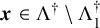 , there are some
$L\in \{N_1, L_1, L_0\}$
, there are some
$L\in \{N_1, L_1, L_0\}$
 and some
$\mathcal {ER}(L)\ni W\subset \Lambda ^{\dagger }\setminus \Lambda ^{\dagger }_1$
and some
$\mathcal {ER}(L)\ni W\subset \Lambda ^{\dagger }\setminus \Lambda ^{\dagger }_1$
 so that

Proof. The proof is similar to that of Theorem 3.7 of [Reference Jitomirskaya, Liu and ShiJLS20] (cf. pages 471–472). We initially set
$Q^\dagger =(\boldsymbol {k}_*+[-L_3, L_3]^b)\times [-L_2, L_2]^d$
 and
$Q_1=(\boldsymbol {k}_*+[-L_1, L_1]^b)\times [-L_1, L_1]^d$
and
$Q_1=(\boldsymbol {k}_*+[-L_1, L_1]^b)\times [-L_1, L_1]^d$
 . Then we slightly change
$Q^\dagger , Q_1^\dagger $
. Then we slightly change
$Q^\dagger , Q_1^\dagger $
 to
$\Lambda ^\dagger , \Lambda _1^\dagger $
to
$\Lambda ^\dagger , \Lambda _1^\dagger $
 with the diameter modulations of length
$2L_1$
with the diameter modulations of length
$2L_1$
 if the boundary of
$Q^\dagger , Q_1^\dagger $
if the boundary of
$Q^\dagger , Q_1^\dagger $
 approaches the boundary of
$\mathcal R_1$
approaches the boundary of
$\mathcal R_1$
 with the distance of
$0<L\leq 2L_1$
with the distance of
$0<L\leq 2L_1$
 .
.
Next, let
$\boldsymbol {x}=(\boldsymbol {k}, \boldsymbol {n})\in \Lambda ^{\dagger }\setminus \Lambda _1^{\dagger }$
 . For
$|\boldsymbol {n}|\leq 10N_1$
. For
$|\boldsymbol {n}|\leq 10N_1$
 , we use
$L_1$
, we use
$L_1$
 size regions to cover
$\boldsymbol {x}$
size regions to cover
$\boldsymbol {x}$
 ; for
$10N_1<|\boldsymbol {n}|\leq L_1$
; for
$10N_1<|\boldsymbol {n}|\leq L_1$
 , we use the
$N_1$
, we use the
$N_1$
 size regions to cover
$\boldsymbol {x}$
size regions to cover
$\boldsymbol {x}$
 ; for
$L_1< |\boldsymbol {n}|\leq L_2$
; for
$L_1< |\boldsymbol {n}|\leq L_2$
 , we use the
$L_0$
, we use the
$L_0$
 size regions to cover
$\boldsymbol {x}.$
size regions to cover
$\boldsymbol {x}.$

Next, we show that all
$Q\in (\boldsymbol {k}, \boldsymbol {0})+\mathcal {ER}_{\boldsymbol {0}}(L_1)$
 satisfying
$|\boldsymbol {k}|\leq N$
satisfying
$|\boldsymbol {k}|\leq N$
 and
$|\boldsymbol {k}-\boldsymbol {k}_*|>10N_1$
and
$|\boldsymbol {k}-\boldsymbol {k}_*|>10N_1$
 are
$\sigma $
are
$\sigma $
 -good for “most”
$\sigma $
-good for “most”
$\sigma $
 , by using Cartan’s lemma and coupling lemma of [Reference LiuLiu22]. More precisely, we have
Lemma 2.29. Let
$\boldsymbol {\omega }\in \widetilde \Omega _N\cap \Omega _{N_2}$
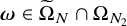 . There is some
$\tilde \Sigma _{N,2}\subset \mathbb R$
. There is some
$\tilde \Sigma _{N,2}\subset \mathbb R$
 satisfying

so that for
$\sigma \notin \tilde \Sigma _{N, 2}$
 , the following holds true. If
$Q\subset \mathcal R_1$
, the following holds true. If
$Q\subset \mathcal R_1$
 satisfies

then Q is
$\sigma $
 -good with
$\gamma _{L_1}=\gamma _{N_1}-N_1^{-\vartheta }$
-good with
$\gamma _{L_1}=\gamma _{N_1}-N_1^{-\vartheta }$
 , where
$\vartheta>0$
, where
$\vartheta>0$
 is an absolute constant defined in Lemma B.3.
Proof of Lemma 2.29
We choose any
$Q\in \mathcal {ER}(L_1)$
 with
$Q\in \mathcal Q$
with
$Q\in \mathcal Q$
 . Then we take any
$Q'\in \mathcal R_{L_*}^{{\sqrt {L_1}}}$
. Then we take any
$Q'\in \mathcal R_{L_*}^{{\sqrt {L_1}}}$
 satisfying
$Q'\subset Q$
satisfying
$Q'\subset Q$
 and
$\sqrt {{L_1}}\leq L_*\leq 2L_1$
and
$\sqrt {{L_1}}\leq L_*\leq 2L_1$
 . From Lemma 2.22 and
$\boldsymbol {\omega }\in \widetilde \Omega _N$
. From Lemma 2.22 and
$\boldsymbol {\omega }\in \widetilde \Omega _N$
 , we have for any
$\sigma \in \mathbb R,$
, we have for any
$\sigma \in \mathbb R,$


Denote by
$Y_1(\sigma ):=\bigcup \limits _{1\leq \ell \leq k} Q_{\boldsymbol {x}_\ell }, k\leq N^{\frac {1}{10^3(b+d)^2}}$
 all those
$\sigma $
all those
$\sigma $
 -bad
$N_1$
-bad
$N_1$
 size elementary regions. We claim that, there is some
$Y=Y(\sigma )\subset Q'$
size elementary regions. We claim that, there is some
$Y=Y(\sigma )\subset Q'$
 satisfying
$\#Y\leq C(b,d)N_1^{b+d} N^{\frac {1}{10^3(b+d)^2}}$
satisfying
$\#Y\leq C(b,d)N_1^{b+d} N^{\frac {1}{10^3(b+d)^2}}$
 , so that if
$\boldsymbol {x}\in Q'\setminus Y$
, so that if
$\boldsymbol {x}\in Q'\setminus Y$
 , then there is some
$\sigma $
, then there is some
$\sigma $
 -good
$W\in \mathcal {ER}(N_1), W\subset Q'\setminus Y$
-good
$W\in \mathcal {ER}(N_1), W\subset Q'\setminus Y$
 satisfying

Indeed, we pave
$Q'$
 with
$\Lambda _\alpha $
with
$\Lambda _\alpha $
 for
$\Lambda _\alpha =Q'\cap \Lambda _{10N_1}(\boldsymbol {x}), \boldsymbol {x}\in 10N_1\mathbb Z^{b+d}$
for
$\Lambda _\alpha =Q'\cap \Lambda _{10N_1}(\boldsymbol {x}), \boldsymbol {x}\in 10N_1\mathbb Z^{b+d}$
 . Then we can enlarge
$\Lambda _\alpha $
. Then we can enlarge
$\Lambda _\alpha $
 to
$\tilde \Lambda _\alpha \subset Q'$
to
$\tilde \Lambda _\alpha \subset Q'$
 so that
$\tilde \Lambda _\alpha $
so that
$\tilde \Lambda _\alpha $
 has width at least
$N_1$
has width at least
$N_1$
 and diameter at most
$C(b,d)N_1$
and diameter at most
$C(b,d)N_1$
 , and
$\bigcup \limits _{\alpha }\tilde \Lambda _\alpha $
, and
$\bigcup \limits _{\alpha }\tilde \Lambda _\alpha $
 remains a tiling of
$Q'$
remains a tiling of
$Q'$
 . It suffices to take

Since each
$Q_{\boldsymbol {x}_\ell }$
 can only intersect with at most
$C(b,d)$
can only intersect with at most
$C(b,d)$
 many
$\tilde \Lambda _\alpha $
many
$\tilde \Lambda _\alpha $
 , we have

We are ready to apply Cartan’s lemma (cf. Lemma 2.25). From Lemma B.1, any
$\sigma $
 -good
$N_1$
-good
$N_1$
 region remains essentially
$\sigma '$
region remains essentially
$\sigma '$
 -good if
$|\sigma '-\sigma |\leq e^{-10\gamma N_1}$
-good if
$|\sigma '-\sigma |\leq e^{-10\gamma N_1}$
 . So on an interval I of length at most
$e^{-10\gamma N_1}$
. So on an interval I of length at most
$e^{-10\gamma N_1}$
 , we can fix Y to associate with the midpoint of I. In addition, we can assume
$|\sigma |\leq C(b,d)N$
, we can fix Y to associate with the midpoint of I. In addition, we can assume
$|\sigma |\leq C(b,d)N$
 since if
$|\sigma |>CN$
since if
$|\sigma |>CN$
 , then
$\|D_{Q'}^{-1}(\sigma )\|\leq 1$
, then
$\|D_{Q'}^{-1}(\sigma )\|\leq 1$
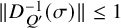 . In this case,
$Q'$
. In this case,
$Q'$
 becomes
$\sigma $
becomes
$\sigma $
 -good via the Neumann series argument. We apply Lemma 2.25 with

It remains to verify the assumptions of Lemma 2.25. First, one has by the definition of the operator
$H(\sigma ),$


We let Y be defined in the above claim. Then using sublinear bound conclusion and Lemma B.5, we have

To apply the matrix-valued Cartan’s lemma, we need the scale

Recall that the LDE hold at scale
$N_2$
 . Applying the resolvent identity Lemma B.5 and using (2) of Lemma 2.23 with
$L=N_2$
. Applying the resolvent identity Lemma B.5 and using (2) of Lemma 2.23 with
$L=N_2$
 yield
yield

for
$\sigma $
 away from a set of measure at most (since
$0<\rho <c_2\kappa _1$
away from a set of measure at most (since
$0<\rho <c_2\kappa _1$
 )
)

It follows from
$N_1=N_2^{\frac \rho 2}$
 that
that

This verifies (iii) of Lemma 2.25. If
$\epsilon =e^{- {L_*}^{\frac {1}{2}}}$
 , then one has
$\epsilon <(1+K_1+K_2)^{-10M}.$
, then one has
$\epsilon <(1+K_1+K_2)^{-10M}.$
 Cover
$[-CN, CN]$
Cover
$[-CN, CN]$
 with disjoint intervals of length
$e^{- 10\gamma N_1}$
with disjoint intervals of length
$e^{- 10\gamma N_1}$
 . Define

Then by (2.30) of Lemma 2.25, one obtains

Note that the number of
$Q'\subset Q$
 with
$Q'\in \mathcal {R}_{L_*}^{\sqrt {L_1}}, \sqrt {{L_1}}\leq L_*\leq 2L_1$
with
$Q'\in \mathcal {R}_{L_*}^{\sqrt {L_1}}, \sqrt {{L_1}}\leq L_*\leq 2L_1$
 is at most
$L^{C(b,d)}$
is at most
$L^{C(b,d)}$
 and the number of
$Q\in \mathcal Q$
and the number of
$Q\in \mathcal Q$
 is at most
$N^{(b,d)}$
is at most
$N^{(b,d)}$
 . We take the union over all these
$Q'\subset Q, Q\in \mathcal Q$
. We take the union over all these
$Q'\subset Q, Q\in \mathcal Q$
 leading to the desired
$\tilde \Sigma _{N,2}\subset \mathbb R$
leading to the desired
$\tilde \Sigma _{N,2}\subset \mathbb R$
 with (since
$0<\rho <c_2\leq \frac {1}{10^4(b+d)^2}$
with (since
$0<\rho <c_2\leq \frac {1}{10^4(b+d)^2}$
 )
)

To finish the proof, it suffices to prove the off-diagonal exponential decay of
$G_Q(\sigma )$
 for
$Q\in \mathcal Q$
for
$Q\in \mathcal Q$
 and
$\sigma \notin \tilde \Sigma _{N,2}$
and
$\sigma \notin \tilde \Sigma _{N,2}$
 . This follows from using the coupling lemma of [Reference LiuLiu22]. Indeed, fix
$Q\in \mathcal Q$
. This follows from using the coupling lemma of [Reference LiuLiu22]. Indeed, fix
$Q\in \mathcal Q$
 (then
$Q\in \mathcal {ER}(L_1)$
(then
$Q\in \mathcal {ER}(L_1)$
 ). Let
$\mathcal F$
). Let
$\mathcal F$
 be any family of pairwise disjoint
$\sqrt {L_1}$
be any family of pairwise disjoint
$\sqrt {L_1}$
 size elementary regions in Q. Then using Lemma 2.22 and
$\boldsymbol {\omega }\in \widetilde \Omega _N,$
size elementary regions in Q. Then using Lemma 2.22 and
$\boldsymbol {\omega }\in \widetilde \Omega _N,$
 we get

So applying Lemma B.3 leads to the off-diagonal exponential decay of
$G_Q(\sigma )$
 with the decay rate

We then deal with
$G_{\Lambda ^{\dagger }}(\sigma )$
 with
$\Lambda ^{\dagger }$
with
$\Lambda ^{\dagger }$
 given by Lemma 2.28. We have
Lemma 2.30. Let
$\boldsymbol {\omega }\in \widetilde \Omega _N\cap \Omega _{N_2}$
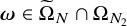 . Then there is some
$\widetilde \Sigma _{N, 3}\subset \mathbb R$
. Then there is some
$\widetilde \Sigma _{N, 3}\subset \mathbb R$
 satisfying

so that, if
$\sigma \notin \bigcup \limits _{\ell =1, 2,3}\tilde \Sigma _{N,\ell },$
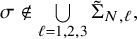 then
$G_{\Lambda ^{\dagger }}(\sigma )$
then
$G_{\Lambda ^{\dagger }}(\sigma )$
 is
$\sigma $
is
$\sigma $
 -good in the sense of Definition 2.21 (replacing
$\Lambda $
-good in the sense of Definition 2.21 (replacing
$\Lambda $
 with
$\Lambda ^\dagger $
with
$\Lambda ^\dagger $
 ) with
$\gamma _{L_2}=\gamma _{L_1}-N_1^{-\frac {1}{10}}$
) with
$\gamma _{L_2}=\gamma _{L_1}-N_1^{-\frac {1}{10}}$
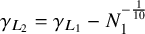 .
.
Proof of Lemma 2.30
The proof is similar to that of Lemma 2.29, but is more in the spirit of [Reference Jitomirskaya, Liu and ShiJLS20] when dealing with off-diagonal exponential decay estimate, as
$\Lambda ^{\dagger }$
 has the special annulus structure.
To get the sub-exponential growth estimate of
$\|G_{\Lambda ^\dagger }(\sigma )\|$
 , the key point is to apply Cartan’s lemma only involving
$N_1, N_2$
, the key point is to apply Cartan’s lemma only involving
$N_1, N_2$
 sizes regions similar to the proof of Lemma 2.29. This means precisely that we do not choose
$Y=\Lambda _1^\dagger $
sizes regions similar to the proof of Lemma 2.29. This means precisely that we do not choose
$Y=\Lambda _1^\dagger $
 when applying Lemma 2.25.
From
$\boldsymbol {\omega }\in \widetilde \Omega _N$
 , the definition of
$\Lambda ^\dagger $
, the definition of
$\Lambda ^\dagger $
 (cf. Lemma 2.28) and Lemma 2.22, we have for any
$\sigma \in \mathbb R,$
(cf. Lemma 2.28) and Lemma 2.22, we have for any
$\sigma \in \mathbb R,$


Similar to the proof of Lemma 2.29, we can find some
$Y=Y(\sigma )\subset \Lambda ^\dagger $
 satisfying
$\#Y\leq C(b,d)N^{2\rho ^2(b+d)} N^{\frac {1}{50(b+d)}}<N^{\frac {1}{49(b+d)}}$
satisfying
$\#Y\leq C(b,d)N^{2\rho ^2(b+d)} N^{\frac {1}{50(b+d)}}<N^{\frac {1}{49(b+d)}}$
 so that, if
$\boldsymbol {x}\in \Lambda ^\dagger \setminus Y$
so that, if
$\boldsymbol {x}\in \Lambda ^\dagger \setminus Y$
 , then there is some
$\sigma $
, then there is some
$\sigma $
 -good
$W\in \mathcal {ER}(N_1), W\subset \Lambda ^\dagger \setminus Y$
-good
$W\in \mathcal {ER}(N_1), W\subset \Lambda ^\dagger \setminus Y$
 satisfying

Let
$\boldsymbol {\omega }\in \widetilde \Omega _N$
 . Again, both the site
$\boldsymbol {k}_*\in [-N, N]^b$
. Again, both the site
$\boldsymbol {k}_*\in [-N, N]^b$
 (given in Lemma 2.26) and
$Y(\sigma )$
(given in Lemma 2.26) and
$Y(\sigma )$
 depend on
$\sigma $
depend on
$\sigma $
 . From Lemma B.1, any
$\sigma $
. From Lemma B.1, any
$\sigma $
 -good
$N_1$
-good
$N_1$
 size region remains essentially
$\sigma '$
size region remains essentially
$\sigma '$
 -good if
$|\sigma '-\sigma |\leq e^{-10\gamma N_1}$
-good if
$|\sigma '-\sigma |\leq e^{-10\gamma N_1}$
 . So on an interval I of length at most
$e^{-10\gamma N_1}$
. So on an interval I of length at most
$e^{-10\gamma N_1}$
 , we can choose
$Y, \boldsymbol {k}_*$
, we can choose
$Y, \boldsymbol {k}_*$
 to associate with the midpoint of I. Also, we can assume
$|\sigma |\leq C(b,d)N$
to associate with the midpoint of I. Also, we can assume
$|\sigma |\leq C(b,d)N$
 since if
$|\sigma |>CN$
since if
$|\sigma |>CN$
 , then
$\|D_{\Lambda ^\dagger }^{-1}(\sigma )\|\leq 1$
, then
$\|D_{\Lambda ^\dagger }^{-1}(\sigma )\|\leq 1$
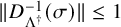 , and
$\Lambda ^\dagger $
, and
$\Lambda ^\dagger $
 becomes
$\sigma $
becomes
$\sigma $
 -good via the Neumann series argument.
We now apply Lemma 2.25 with

We have
$ K_1=C N. $
 Using the sublinear bound conclusion and the resolvent identity Lemma B.5, we have

We again use the scale
$N_2=N_1^{\frac 2\rho }$
 , at which the LDE hold. Similar to the proof of Lemma 2.29, we can verify all assumptions of Lemma 2.25. Define

Then by (2.30) of Lemma 2.25, one obtains

Finally, it suffices to prove the off-diagonal exponential decay of
$G_{\Lambda ^\dagger }(\sigma ).$
 This follows directly from the resolvent identity of [Reference Jitomirskaya, Liu and ShiJLS20], that is, Lemma B.6. In fact, by the analysis in
$\mathcal R_2$
This follows directly from the resolvent identity of [Reference Jitomirskaya, Liu and ShiJLS20], that is, Lemma B.6. In fact, by the analysis in
$\mathcal R_2$
 , Lemma 2.29 and Lemma 2.28, all elementary regions contained in
$\Lambda ^\dagger \setminus \Lambda _1^\dagger $
, Lemma 2.29 and Lemma 2.28, all elementary regions contained in
$\Lambda ^\dagger \setminus \Lambda _1^\dagger $
 with sizes
$N_1, L_0, L_1$
with sizes
$N_1, L_0, L_1$
 are
$\sigma $
are
$\sigma $
 -good. Then applying Lemma B.6 with
$\Lambda =\Lambda ^\dagger , \Lambda _1=\Lambda _1^\dagger $
-good. Then applying Lemma B.6 with
$\Lambda =\Lambda ^\dagger , \Lambda _1=\Lambda _1^\dagger $
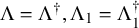 (since
$\mathrm {diam}\ \Lambda ^\dagger \sim L_3>100^{2(b+d)} L_1^{2(b+d)}\geq (\mathrm {diam}\ \Lambda _1^\dagger )^{2(b+d)}$
(since
$\mathrm {diam}\ \Lambda ^\dagger \sim L_3>100^{2(b+d)} L_1^{2(b+d)}\geq (\mathrm {diam}\ \Lambda _1^\dagger )^{2(b+d)}$
 ) leads to the desired off-diagonal exponential decay estimate of
$G_{\Lambda ^\dagger }(\sigma )$
) leads to the desired off-diagonal exponential decay estimate of
$G_{\Lambda ^\dagger }(\sigma )$
 with
with

Application of the resolvent identity again
The distribution of resonant blocks.

Figure 1 Long description
At the center is a blue hatched square intersected by horizontal and vertical bands of small red squares labeled S. Surrounding this are four nested rectangles: the innermost green, the next orange, then a larger blue, and the largest black. Each rectangle is annotated with a scale: L sub 0 is approximately L sub 1 to the 9 all over 10 power, L sub 1 is approximately N to the 1 all over 100 times open parenthesis b plus d close parenthesis squared, L sub 2 is approximately N to the 50 all over open parenthesis b plus d close parenthesis squared, and L sub 3 is approximately N to the 1 all over 10 times open parenthesis b plus d close parenthesis. The axes at top left are labeled k (vertical) and n (horizontal). The horizontal axis is marked with log N sub 1 much less than log N and extends to greater than 10 N sub 1. The right side shows an enlarged orange square with a dot, labeled L sub 0. Dashed lines and colored boxes indicate the spatial distribution and scaling of resonant blocks.
Finally, we define
$\Sigma _{N}=\bigcup \limits _{\ell =1,2,3}\tilde \Sigma _{N, \ell }$
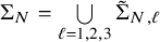 with
$\tilde \Sigma _{N, 1}, \tilde \Sigma _{N, 2}, \tilde \Sigma _{N, 3}$
with
$\tilde \Sigma _{N, 1}, \tilde \Sigma _{N, 2}, \tilde \Sigma _{N, 3}$
 given by the analysis in
$\mathcal R_2$
given by the analysis in
$\mathcal R_2$
 , Lemma 2.29, Lemma 2.30, respectively. Then

and for
$\sigma \notin \Sigma _N$
 , we can cover
$\Lambda _{\mathrm {pm}, N}$
, we can cover
$\Lambda _{\mathrm {pm}, N}$
 with
$\sigma $
with
$\sigma $
 -good regions of sizes
$N_1, L_0, L_1, L_3$
-good regions of sizes
$N_1, L_0, L_1, L_3$
 . More precisely, we have (cf. Figure 1)
-
○ For $\boldsymbol {x}\in \mathcal R_2$
, cover
$\boldsymbol {x}$
with
$\Lambda \in \mathcal {ER}(L_0)$
with
$L_0\sim N^{\frac {9}{1000(b+d)^2}}$
. -
○ For $\boldsymbol {x}\in \Lambda _1^\dagger $
, cover
$\boldsymbol {x}$
with
$\Lambda ^\dagger $
. -
○ For $\boldsymbol {x}\in \mathcal R_1\setminus \Lambda _1^\dagger $
, cover
$\boldsymbol {x}$
with regions in $$ \begin{align*}\bigcup_{L=N_1, L_0, L_1}\mathcal{ER}(L).\end{align*} $$



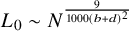


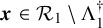


As a result, for
$\sigma \notin \Sigma _N$
 , we can apply Lemma B.5 and Lemma B.6 to show that
$\Lambda _{\mathrm {pm}, N}$
, we can apply Lemma B.5 and Lemma B.6 to show that
$\Lambda _{\mathrm {pm}, N}$
 is
$\sigma $
is
$\sigma $
 -good. Indeed, we first apply Lemma B.5 with

to obtain

Next, for the off-diagonal exponential decay, we use Lemma B.6 with
$\Lambda =\Lambda _{\mathrm {pm}, N},\ \Lambda _1=\emptyset $
 ,
$M_0=N_1$
,
$M_0=N_1$
 to obtain (recalling the decay rate estimates in Lemmas 2.29, 2.30) for
$|\boldsymbol {x}-\boldsymbol {x}'|>N^{\frac 89},$
to obtain (recalling the decay rate estimates in Lemmas 2.29, 2.30) for
$|\boldsymbol {x}-\boldsymbol {x}'|>N^{\frac 89},$
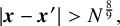

where

Since
$N\sim N_1^{\frac {1}{\rho ^2}}$
 , we choose
$\ell _*$
, we choose
$\ell _*$
 so that
$N^{\rho ^{2\ell _*}}:=N_*\sim \log ^{\frac 1\kappa }\frac {1}{\varepsilon +\delta }$
so that
$N^{\rho ^{2\ell _*}}:=N_*\sim \log ^{\frac 1\kappa }\frac {1}{\varepsilon +\delta }$
 . It follows from applying Lemma 2.15 (i.e.,
$\gamma _{N^{\rho ^{2\ell _*}}}=\gamma _0=\gamma -\log ^{-2}\frac {1}{\varepsilon +\delta }$
. It follows from applying Lemma 2.15 (i.e.,
$\gamma _{N^{\rho ^{2\ell _*}}}=\gamma _0=\gamma -\log ^{-2}\frac {1}{\varepsilon +\delta }$
 ) and iterating (2.35) that

provided
$0<\varepsilon +\delta \leq c(\rho , c_1, \kappa ).$

The above arguments hold indeed for all scales in
$[N, N^2]$
 . Then we can propagate the LDE from small scales interval
$[N_1, N_2]$
. Then we can propagate the LDE from small scales interval
$[N_1, N_2]$
 to large scales one
$[N, N^2]$
to large scales one
$[N, N^2]$
 similar to the proof of Theorem 4.1 in [Reference Jitomirskaya, Liu and ShiJLS20]. This completes the proof of Lemma 2.20.

3 Nonlinear analysis
In this section, we focus on nonlinear analysis. We work directly with the nonlinear equation (1.1). Recall that

We aim to construct solutions to (1.1) of the form

Using the ansatz, we get the nonlinear lattice equation

where
$\hat v(\boldsymbol {k},\boldsymbol {n})=\overline {\hat u(-\boldsymbol {k}, \boldsymbol {n})}$
 , the convolution is only in the
$\boldsymbol {k}$
, the convolution is only in the
$\boldsymbol {k}$
 -variable:

and

Note that
$\Delta $
 acts only on the
$\boldsymbol {n}$
acts only on the
$\boldsymbol {n}$
 -variable. To solve for
$\hat u, \hat v$
-variable. To solve for
$\hat u, \hat v$
 , we also need a conjugate equation of (3.1):

As a result, we obtain the following vector-valued nonlinear lattice equation:

where

with

and

The linearized operator of P at
$\vec u$
 is then given by

3.1 The Lyapunov-Schmidt decomposition
We look for quasi-periodic solutions to (1.1) near

using the Lyapunov-Schmidt decomposition. The Fourier support of
$u^{(0)}$
 is
$\mathcal {S}_+=\{(\boldsymbol {e}_\ell , \boldsymbol {n}_\ell )_{\ell =1}^b\}\subset \mathbb Z^{b+d}$
is
$\mathcal {S}_+=\{(\boldsymbol {e}_\ell , \boldsymbol {n}_\ell )_{\ell =1}^b\}\subset \mathbb Z^{b+d}$
 (we identify
$ \mathcal {S}_+$
(we identify
$ \mathcal {S}_+$
 with
$\{(\boldsymbol {e}_\ell , \boldsymbol {n}_\ell )_{\ell =1}^b\}\times \{+\}\subset \mathbb Z^{b+d}_{\mathrm {pm}}$
with
$\{(\boldsymbol {e}_\ell , \boldsymbol {n}_\ell )_{\ell =1}^b\}\times \{+\}\subset \mathbb Z^{b+d}_{\mathrm {pm}}$
 ). Similarly, let
$\mathcal {S}_-=\{(-\boldsymbol {e}_\ell , \boldsymbol {n}_\ell )_{\ell =1}^b\}\subset \mathbb Z^{b+d}$
). Similarly, let
$\mathcal {S}_-=\{(-\boldsymbol {e}_\ell , \boldsymbol {n}_\ell )_{\ell =1}^b\}\subset \mathbb Z^{b+d}$
 be the Fourier support of
$v^{(0)}:=\overline {u^{(0)}}$
be the Fourier support of
$v^{(0)}:=\overline {u^{(0)}}$
 , which is then identified with
$\{(-\boldsymbol {e}_\ell , \boldsymbol {n}_\ell )_{\ell =1}^b\}\times \{-\}\subset \mathbb Z^{b+d}_{\mathrm {pm}}$
, which is then identified with
$\{(-\boldsymbol {e}_\ell , \boldsymbol {n}_\ell )_{\ell =1}^b\}\times \{-\}\subset \mathbb Z^{b+d}_{\mathrm {pm}}$
 . Let
$\mathcal {S}=\mathcal {S}_+\cup \mathcal {S}_-$
. Let
$\mathcal {S}=\mathcal {S}_+\cup \mathcal {S}_-$
 and write
$\mathbb Z^{b+d}_{\mathrm {pm}, *}=\mathbb Z^{b+d}_{\mathrm {pm}}\setminus \mathcal {S}:=\mathcal S^c.$
and write
$\mathbb Z^{b+d}_{\mathrm {pm}, *}=\mathbb Z^{b+d}_{\mathrm {pm}}\setminus \mathcal {S}:=\mathcal S^c.$

We divide the equation (3.2) into the P-equations

and the Q-equations

We iteratively solve the Q-equations and then the P-equations.
3.2 The Q-equations and extraction of parameters
The Q-equations are
$2b$
 -dimensional.
On
$\mathcal S$
 ,
$\vec u$
,
$\vec u$
 is held fixed, and the Q-equations (3.6) are viewed instead as equations for
$\boldsymbol {\omega }$
is held fixed, and the Q-equations (3.6) are viewed instead as equations for
$\boldsymbol {\omega }$
 , and will be solved using the implicit function theorem. The Q-equations are used to relate the frequencies
$\boldsymbol {\omega }$
, and will be solved using the implicit function theorem. The Q-equations are used to relate the frequencies
$\boldsymbol {\omega }$
 to the amplitudes
$\boldsymbol {a}$
to the amplitudes
$\boldsymbol {a}$
 , permitting amplitude-frequency modulation to solve the P-equations.
Note that

where

The solutions
$\vec u=(\hat u, \hat v)^t$
 (with
$(\cdot )^t$
(with
$(\cdot )^t$
 denoting the transpose) on
$\mathcal S$
denoting the transpose) on
$\mathcal S$
 are held fixed:
$\vec u \equiv (\hat u^{(0)}, \hat v^{(0)})^t=\vec u^{(0)}$
are held fixed:
$\vec u \equiv (\hat u^{(0)}, \hat v^{(0)})^t=\vec u^{(0)}$
 on
$\mathcal S$
on
$\mathcal S$
 , the Q-equations are used instead to solve for the frequencies. Due to symmetry, the Q-equations for
$\hat v$
, the Q-equations are used instead to solve for the frequencies. Due to symmetry, the Q-equations for
$\hat v$
 are the same as those for
$\hat u$
are the same as those for
$\hat u$
 . So we only need to consider those for
$\hat u$
. So we only need to consider those for
$\hat u$
 . Solving the equations at the initial step

leads to, for
$1\leq \ell \leq b$
 , the initial modulated frequencies

satisfying

Along the way, we will show that
$\boldsymbol {\omega }^{(r)}=\boldsymbol {\omega }^{(0)}+O(\delta )$
 , for all
$r=0, 1, 2, \cdots $
, for all
$r=0, 1, 2, \cdots $
 . So
$\boldsymbol {\omega }^{(r)}\in \Omega $
. So
$\boldsymbol {\omega }^{(r)}\in \Omega $
 , the frequency set in Theorem 2.11, hence Theorem 2.11 is at our disposal to solve the P-equations. To construct approximate solutions to the P-equations, it is convenient to view
$\boldsymbol {\omega }\in \Omega $
, the frequency set in Theorem 2.11, hence Theorem 2.11 is at our disposal to solve the P-equations. To construct approximate solutions to the P-equations, it is convenient to view
$\boldsymbol {\omega }\in \Omega $
 as an independent parameter, and work in the
$(\boldsymbol {\omega }, \boldsymbol {a})$
as an independent parameter, and work in the
$(\boldsymbol {\omega }, \boldsymbol {a})$
 -variable,
$(\boldsymbol {\omega }, \boldsymbol {a})\in \Omega \times [1,2]^b:=(\boldsymbol {\omega }^{(0)}+[\delta , 2^{2p}\delta ]^b)\times [1,2]^b$
-variable,
$(\boldsymbol {\omega }, \boldsymbol {a})\in \Omega \times [1,2]^b:=(\boldsymbol {\omega }^{(0)}+[\delta , 2^{2p}\delta ]^b)\times [1,2]^b$
 . The approximate solutions to the nonlinear matrix equation (3.1) will then be obtained by taking into account the solutions to the Q-equations as well, which restricts
$(\boldsymbol {\omega }, \boldsymbol {a})$
. The approximate solutions to the nonlinear matrix equation (3.1) will then be obtained by taking into account the solutions to the Q-equations as well, which restricts
$(\boldsymbol {\omega }, \boldsymbol {a})$
 to the b-dimensional hypersurface
$\boldsymbol {\omega }=\boldsymbol {\omega }^{(r)} (\boldsymbol {a})$
to the b-dimensional hypersurface
$\boldsymbol {\omega }=\boldsymbol {\omega }^{(r)} (\boldsymbol {a})$
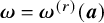 , at the r-th iteration.
3.3 The P-equations
The P-equations are infinite-dimensional.
We use (3.5) to solve for
$\vec u |_{\mathcal S^c}$
 . Solving the P-equations requires analyzing the invertibility of the linearized operator
$H=H_0+\delta T_{\vec u}$
. Solving the P-equations requires analyzing the invertibility of the linearized operator
$H=H_0+\delta T_{\vec u}$
 restricted to
$\mathbb Z^{b+d}_{\mathrm {pm}, *}$
restricted to
$\mathbb Z^{b+d}_{\mathrm {pm}, *}$
 , which we do in the previous section. Then the resolution of the P-equations combines the Newton scheme and the linear analysis in Section 2. The large deviation estimates in
$\sigma $
, which we do in the previous section. Then the resolution of the P-equations combines the Newton scheme and the linear analysis in Section 2. The large deviation estimates in
$\sigma $
 in Theorem 2.11 will be converted into estimates in the amplitudes
$\boldsymbol {a}$
in Theorem 2.11 will be converted into estimates in the amplitudes
$\boldsymbol {a}$
 by using a semi-algebraic projection lemma (cf. Lemma 3.7 below), and amplitude-frequency modulation,
$\boldsymbol {\omega }=\boldsymbol {\omega }(\boldsymbol {a})$
by using a semi-algebraic projection lemma (cf. Lemma 3.7 below), and amplitude-frequency modulation,
$\boldsymbol {\omega }=\boldsymbol {\omega }(\boldsymbol {a})$
 . This is an established scheme, which has recently been extensively elaborated on with detailed proofs in sects. IV-VI, [Reference Kachkovskiy, Liu and WangKLW24] and [Reference Liu and WangLW24]. They will serve as the basic reference point for the present section.
Recall first the formal Newton scheme. Let
$\vec u$
 be an approximate solution to the P-equations (3.5). For the next approximation
${\vec u}'$
be an approximate solution to the P-equations (3.5). For the next approximation
${\vec u}'$
 , write

Then
$\Delta _{\mathrm {cor}}\vec u'$
 is set to be

where the linearized operator
$H(\vec u)=H_0+\delta T_{\vec u}(\boldsymbol {\omega }, \boldsymbol {a})$
 (cf. (3.3) and (3.4)). This is, however, only indicative since we assume that
$H(\vec u)$
(cf. (3.3) and (3.4)). This is, however, only indicative since we assume that
$H(\vec u)$
 is invertible. Due to the small divisor difficulties in the inversion process, we need to regularize the linearized operator
$H(\vec u)$
is invertible. Due to the small divisor difficulties in the inversion process, we need to regularize the linearized operator
$H(\vec u)$
 and do a multi-scale Newton iteration instead.
Toward that purpose, let M be a large integer and consider the geometric sequence of scales
$M^\ell $
 ,
$\ell =1, 2, \cdots $
,
$\ell =1, 2, \cdots $
 . Denote by
$\vec u^{(r)}$
. Denote by
$\vec u^{(r)}$
 , the r-th approximate solution to the P-equations (3.5). For the
$(r+1)$
, the r-th approximate solution to the P-equations (3.5). For the
$(r+1)$
 -th approximation, write

We define (if it exists)

where
$N=M^{r+1}$
 and
$R_{N}$
and
$R_{N}$
 is the restriction operator to the cube
$\Lambda _{N}\cap \mathbb Z^{b+d}_{\mathrm {pm, *}}.$
is the restriction operator to the cube
$\Lambda _{N}\cap \mathbb Z^{b+d}_{\mathrm {pm, *}}.$
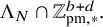 This leads to estimate the inverse (i.e., the Green’s function),

The following estimates are crucial for the convergence of the approximate solutions with exponential decay:

for
$\boldsymbol {x}=(\boldsymbol {k}, \boldsymbol {n})$
 and some
$c, C>0$
and some
$c, C>0$
 , see sect. V, [Reference Kachkovskiy, Liu and WangKLW24].
The LDT, Theorem 2.11, in the previous section plays an essential role in the above Green’s function estimates. The operator
$T_{\vec u}$
 plays the role of S in (2.1) (cf. Remark 2.13 for details). The following lemma implies that
$T_{\vec u}$
plays the role of S in (2.1) (cf. Remark 2.13 for details). The following lemma implies that
$T_{\vec u}$
 satisfies the decay assumption of S (cf. also Remark 2.13). This will then enable us to use Theorem 2.11.
Lemma 3.1.
-
(1) For all $\boldsymbol {k},\boldsymbol {k}', \boldsymbol {k}''\in \mathbb Z^b$
,
$\boldsymbol {n},\boldsymbol {n}'\in \mathbb Z^d$
and
$\xi ,\xi '\in \{+, -\}$
, we have the Toeplitz property in the
$\boldsymbol {k}$
-variable: $$ \begin{align*} T_{\vec u}((\boldsymbol{k}'+\boldsymbol{k}, \boldsymbol{n}, \xi); (\boldsymbol{k}"+\boldsymbol{k}, \boldsymbol{n}', \xi'))=T_{\vec u}((\boldsymbol{k}', \boldsymbol{n}, \xi ); (\boldsymbol{k}", \boldsymbol{n}', \xi')). \end{align*} $$
-
(2) Assume that $|\vec u(\boldsymbol {k}, \boldsymbol {n})|\leq e^{-c(|\boldsymbol {k}|+|\boldsymbol {n}|)}, c>0$
. Then we have for some
$C=C(b, p)>0,$
$$ \begin{align*} |T_{\vec u}((\boldsymbol{k}, \boldsymbol{n}, \xi); (\boldsymbol{k}', \boldsymbol{n}', \xi'))|\leq C(1+|\boldsymbol{k}-\boldsymbol{k}'|)^{C} e^{-c|\boldsymbol{k}-\boldsymbol{k}'|-c|\boldsymbol{n}|}\delta_{\boldsymbol{n},\boldsymbol{n}'}. \end{align*} $$








Proof. The proof is similar to that of Lemma 5.1 in [Reference Liu and WangLW24] and Proposition 4.1 in [Reference Liu, Shi and ZhangLSZ25] (our case is easier since the convolution here involves only the
$\boldsymbol {k}$
 -variable). We omit the details.
3.4 The induction hypothesis and the proof
Let M be a large integer and recall that
$\Lambda _{R}\subset \mathbb Z^{b+d}$
 denotes the
$\ell ^\infty $
denotes the
$\ell ^\infty $
 -norm-induced cube of radius R and centered at the origin.
In the following,
$C>0$
 is a large constant and
$c>0$
is a large constant and
$c>0$
 is a small one.
We begin with the analysis of initial induction steps, which relies on the Neumann series argument and Diophantine estimates (2.5) of Theorem 2.2.
3.4.1 The initial
$2r_\star -r_0$
steps

We choose
$1<r_0<r_\star $
 such that

and

where
$c_1>0$
 is given in Theorem 2.11.
Let
$\vec u^{(0)}(\boldsymbol {\omega },\boldsymbol {a})=\vec u^{(0)}(\boldsymbol {\omega }^{(0)},\boldsymbol {a})$
 with
$\boldsymbol {\omega }=\boldsymbol {\omega }^{(1)}$
with
$\boldsymbol {\omega }=\boldsymbol {\omega }^{(1)}$
 given by (3.8).
We start by constructing
$\vec u_{\mathrm {in}}^{(1)}(\boldsymbol {\omega }, \boldsymbol {a})$
 . Obviously,

and (the support)
$\mathrm {supp}\ {F}(\vec u^{(0)})\subset \Lambda _{M_0}$
 for some
$M_0=M_0(p, \mathcal {S})>0.$
for some
$M_0=M_0(p, \mathcal {S})>0.$
 Let
$L_1=M^{r_0+1}>M_0.$
Let
$L_1=M^{r_0+1}>M_0.$
 It suffices to estimate

It follows from (2.5) of Theorem 2.2,
$\boldsymbol {\omega }=\boldsymbol {\omega }^{(0)}+O(\delta )$
 and the Neumann series argument (cf. Lemma B.1) that

since
$L_1=M^{r_0+1}\ll (\varepsilon +\delta )^{-c_1}$
 . Then we have

and consequently

Substituting
$\vec u_{\mathrm {in}}^{(1)}$
 into the Q-equations using

we obtain

Since the second and the third terms are smooth in
$\boldsymbol {\omega }$
 and
$\boldsymbol {a}$
and
$\boldsymbol {a}$
 , using the implicit function theorem yields
$\boldsymbol {\omega }_{\mathrm {in}}^{(2)}=\boldsymbol {\omega }_{\mathrm {in}}^{(2)}(\boldsymbol {a})=(\omega _{\mathrm {in}, \ell }^{(2)}(\boldsymbol {a}))_{\ell =1}^b$
, using the implicit function theorem yields
$\boldsymbol {\omega }_{\mathrm {in}}^{(2)}=\boldsymbol {\omega }_{\mathrm {in}}^{(2)}(\boldsymbol {a})=(\omega _{\mathrm {in}, \ell }^{(2)}(\boldsymbol {a}))_{\ell =1}^b$
 , written in the form:

with a smooth function
$\varphi _{\mathrm {in}, \ell }^{(2)}$
 (comparing with (3.8)).
The above constructions can be inductively performed for
$2r_\star -r_0$
 steps, with
$r_\star $
steps, with
$r_\star $
 satisfying (3.9). So we have obtained
$\vec u_{\mathrm {in}}^{(r)}=\vec u_{\mathrm {in}}^{(r)}(\boldsymbol {\omega }, \boldsymbol {a})$
satisfying (3.9). So we have obtained
$\vec u_{\mathrm {in}}^{(r)}=\vec u_{\mathrm {in}}^{(r)}(\boldsymbol {\omega }, \boldsymbol {a})$
 (
$1\leq r\leq 2r_\star -r_0$
(
$1\leq r\leq 2r_\star -r_0$
 ) for all
$(\boldsymbol {\omega }, \boldsymbol {a})\in \Omega \times [1,2]^b$
) for all
$(\boldsymbol {\omega }, \boldsymbol {a})\in \Omega \times [1,2]^b$
 .
.
3.4.2 The Inductive Theorem
Recall that

We first state the induction hypothesis, which can be verified if
$0<\varepsilon \leq \delta \leq \log ^{-1}\frac {1}{\varepsilon }\leq \delta _0\ll 1$
 and
$(\boldsymbol {\alpha }, \boldsymbol {\theta })\in \mathcal W$
and
$(\boldsymbol {\alpha }, \boldsymbol {\theta })\in \mathcal W$
 (cf. (2.11)). Given its significance, we refer to it as the induction theorem.
Theorem 3.2. For
$r\geq r_\star ,$
 we have
-
(Hi) $\mathrm {supp}\ \vec u^{(r)}\subset \Lambda _{M^{\tilde r}}$
,
$\tilde r=r+r_\star .$
-
(Hii) $\|\Delta _{\mathrm {cor}} \vec u^{(r)}\|<\delta _r,\ \|\partial \Delta _{\mathrm {cor}} \vec u^{(r)}\|<{\bar \delta }_{r}$
, where
$\partial $
refers to derivation in
$\boldsymbol {\omega }$
or
$\boldsymbol {a}$
, $$ \begin{align*}\vec u^{(r)}=\vec u^{(r-1)}+\Delta_{\mathrm{cor}} \vec u^{(r)},\end{align*} $$and $\|\cdot \|=\sup _{\boldsymbol {\omega }, \boldsymbol {a}}\|\cdot \|_{\ell ^2(\mathbb Z_{\mathrm {pm}}^{b+d})}.$
Remark 3.3. The size of $\delta _r, \bar \delta _r$
will satisfy
$\log \log \frac {1}{\delta _r+\bar \delta _r}\sim r.$
-
(Hiii) $|\vec u^{(r)}(\boldsymbol {k}, \boldsymbol {n})|\leq e^{-c(|\boldsymbol {k}|+|\boldsymbol {n}|)}$
for some
$c>0.$
Remark 3.4. The constant $c>0$
will decrease slightly along the iterations but remain bounded away from
$0$
. This will become clear in the proof, cf. sect. V, G. Step 4, [Reference Kachkovskiy, Liu and WangKLW24]. We also remark that
$\vec u ^{(r)}$
can be defined as a
$C^1$
function on the entire parameter space
$(\boldsymbol {\omega }, \boldsymbol {a})\in \Omega \times [1,2]^b$
by using an extension argument, cf., [Reference BourgainBou98, Reference Bourgain and WangBW08] and sect. V, L. Step 9, [Reference Kachkovskiy, Liu and WangKLW24]. So one can apply the implicit function theorem to solve the Q-equations leading to (3.10) $$ \begin{align} \omega_\ell^{(r)}(\boldsymbol{a})=\omega_\ell^{(0)}+(\varepsilon+\delta)\varphi_\ell^{(r)}(\boldsymbol{a}) \ (1\leq \ell\leq b), \end{align} $$
where $\|\partial \boldsymbol {\varphi }^{(r)}\|=\sup _{1\leq \ell \leq b}\|\partial \varphi _\ell ^{(r)}\|\lesssim 1$
and
$ \boldsymbol {\varphi }^{(r)}=( \varphi ^{(r)}_\ell )_{\ell =1}^b.$
By (Hii), we have $$ \begin{align*} |\boldsymbol{\varphi}^{(r)}-\boldsymbol{\varphi}^{(r-1)}|\lesssim (\varepsilon+\delta)\|\vec u^{(r)}-\vec u^{(r-1)}\|\lesssim {(\varepsilon+\delta)}\delta_r. \end{align*} $$
Denote by $\Gamma _r$
the graph of
$\boldsymbol {\omega }^{(r)}=\boldsymbol {\omega }^{(r)}(\boldsymbol {a})$
. We have
$\|\Gamma _r-\Gamma _{r-1}\|\lesssim {(\varepsilon +\delta )}\delta _r.$
Recall that
$\boldsymbol {\omega }$
is given by (3.8) and
$\boldsymbol {\varphi }^{(0)}=\boldsymbol {0}$
. Thus we have a diffeomorphism from
$\boldsymbol {\omega }^{(r)}\in \Omega $
to
$\boldsymbol {a}\in [1,2]^b$
. -
(Hiv) There is a collection $\mathcal {I}_r$
of intervals
$I\subset \Omega \times [1,2]^b$
of size
$M^{-{\tilde r}^{10C}},$
so that-
(a) On each $I\in \mathcal {I}_r,$
both
$\hat u^{(r)}(\boldsymbol {\omega }, \boldsymbol {a})$
and
$ \hat v^{(r)}(\boldsymbol {\omega }, \boldsymbol {a})$
are given by rational functions in
$(\boldsymbol {\omega }, \boldsymbol {a})$
of degree at most
$M^{{\tilde r}^3}$
. -
(b) For $(\boldsymbol {\omega }, \boldsymbol {a})\in \bigcup _{I\in \mathcal {I}_r}I$
, $$ \begin{align*} \|F(\vec u^{(r)})\|\leq \kappa_r,\ \|\partial F(\vec u^{(r)})\|\leq \bar\kappa_r, \end{align*} $$where $\partial $
refers to derivation in
$\boldsymbol {\omega }$
or
$\boldsymbol {a}$
, and
$\log \log \frac {1}{\kappa _r+\bar \kappa _r}\sim r$
.
-
(c) For $(\boldsymbol {\omega }, \boldsymbol {a})\in \bigcup _{I\in \mathcal {I}_r}I$
and
$H=H(\vec u^{(r-1)})$
, one has (3.11) $$ \begin{align} \|H_{M^{\tilde r}}^{-1}\|&\leq M^{{\tilde r}^C}, \end{align} $$
(3.12) $$ \begin{align} |H_{M^{\tilde r}}^{-1}((\boldsymbol{x},\xi); (\boldsymbol{x}',\xi'))|&\leq e^{-c|\boldsymbol{x}-\boldsymbol{x}'|}\ \mathrm{for}\ |\boldsymbol{x}-\boldsymbol{x}'|>{\tilde r}^C, \end{align} $$where $\boldsymbol {x}=(\boldsymbol {k}, \boldsymbol {n}), \boldsymbol {x}'=(\boldsymbol {k}', \boldsymbol {n}')$
and
$H_{M^{\tilde r}}$
refers to the restriction of H to
$\Lambda _{M^{\tilde r}}$
.
-
(d) Each $I\in \mathcal {I}_r$
is contained in some
$I'\in \mathcal {I}_{r-1}$
and $$ \begin{align*} \mathrm{meas}\ \left(\Pi_{\boldsymbol{a}}(\Gamma_{r-1}\cap(\bigcup_{I'\in\mathcal{I}_{r-1}}I'\setminus\bigcup_{I\in\mathcal{I}_r}I))\right)\leq M^{-\frac{\tilde r}{C(b)}}, \end{align*} $$where $C(b)>0$
depends only on b, and
$\Pi _{\boldsymbol {a}}$
denotes the projection of the set on the
$\boldsymbol {a}$
-variable.
-
-
(Hv) The following precise relations hold true
$$ \begin{align*} \delta_r= {(\varepsilon+\delta)}^{\frac{1}{2}}M^{-(\frac{4}{3})^r}, \, \bar\delta_r= {(\varepsilon+\delta)}^{\frac{1}{8}} M^{-\frac{1}{2}(\frac{4}{3})^r};\\ \kappa_r= {(\varepsilon+\delta)}^{\frac{3}{4}} M^{-(\frac{4}{3})^{r+2}}, \, \bar\kappa_r= {(\varepsilon+\delta)}^{\frac{3}{8}} M^{-\frac{1}{2}(\frac{4}{3})^{r+2}}. \end{align*} $$







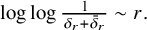






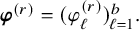












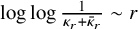







3.5 Proof of the Inductive Theorem
From the analysis in Section 3.4.1, we have constructed
$\vec u_{\mathrm {in }}^{(r)}$
 for
$1\leq r\leq 2r_\star -r_0$
for
$1\leq r\leq 2r_\star -r_0$
 . In particular, we obtain that the Inductive Theorem holds for
$r=r_\star $
. In particular, we obtain that the Inductive Theorem holds for
$r=r_\star $
 as we can set
$\vec u^{(r_\star )}=\vec u_{\mathrm { in}}^{(2r_\star -r_0)}$
as we can set
$\vec u^{(r_\star )}=\vec u_{\mathrm { in}}^{(2r_\star -r_0)}$
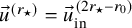 .
.
Assume now the Inductive Theorem holds for
$r>r_\star $
 . We will prove it for
$\ell =r+1.$
. We will prove it for
$\ell =r+1.$

We first check the degree bound on
$\vec u^{(r+1)}$
 (i.e., (Hiv, a) for
$r+1$
(i.e., (Hiv, a) for
$r+1$
 ). In fact, the Newton scheme gives

and by (Hiv, a),
$\vec u^{(r)}(\boldsymbol {\omega }, \boldsymbol {a})$
 is a rational function of degree at most
$M^{\tilde r^3}$
is a rational function of degree at most
$M^{\tilde r^3}$
 (in
$(\boldsymbol {\omega }, \boldsymbol {a})$
(in
$(\boldsymbol {\omega }, \boldsymbol {a})$
 ). By the convolution structure of
$T_{\vec u^{(r)}}$
). By the convolution structure of
$T_{\vec u^{(r)}}$
 , we have

Then by Cramer’s rule, we have

where A is the adjacent matrix of
$H_{N}(\vec u^{(r)})$
 . Hence,

Thus, using (3.13) shows

This proves (Hiv, a) for
$r+1$
 .
.
The other inductive assumptions can be verified in the usual way, cf. [Reference Liu and WangLW24] and sect. V, [Reference Kachkovskiy, Liu and WangKLW24], for example, the verification of (Hiv, b) can be found in I. Step 6 of [Reference Kachkovskiy, Liu and WangKLW24]; the verification of the constant relations (Hv) can be found in Appendix E of [Reference Liu and WangLW24].
It remains to establish (Hiv, c) and (Hiv, d) for
$r+1$
 . For this purpose, we set (recalling
$\tilde r=r+r_\star $
. For this purpose, we set (recalling
$\tilde r=r+r_\star $
 )
)

and a smaller scale,

where
$0<\rho \ll 1$
 is given in Theorem 2.11.
To establish (Hiv, c), we first make approximations on
$T_{\vec u^{(\ell )}}$
 for different
$\vec u^{(\ell )}$
for different
$\vec u^{(\ell )}$
 . For the set

we use
$N_1$
 size regions to do estimates, in order to lower the degree of the associated semi-algebraic set, which will be essential for the upcoming semi-algebraic projection arguments. We set

Then

So we can estimate
$H_{W}^{-1}(\vec u^{(r)})$
 using
$H_Q^{-1}(\vec u^{(r_1)})$
using
$H_Q^{-1}(\vec u^{(r_1)})$
 for
$Q\subset W$
for
$Q\subset W$
 . More precisely, we want to show that the following estimates hold for every
$Q\subset W$
. More precisely, we want to show that the following estimates hold for every
$Q\subset W$
 with
$Q\in \mathcal {ER}(N_1)$
with
$Q\in \mathcal {ER}(N_1)$
 :
:


This requires additional restrictions on
$(\boldsymbol {\omega }, \boldsymbol {a}).$
 For this, we divide into the following cases:
-
Case 1. Assume $Q\in (\boldsymbol {k},\boldsymbol {n})+\mathcal {ER}_0(N_1)$
with
$|\boldsymbol {n}|>10N_1$
and
$Q\subset W.$
Denote by
$\mathcal {C}_1$
the set of all these Q. To estimate
$H_Q^{-1}(\vec u^{(r_1)})$
, we can impose as in the proof of Lemma 2.23 (with
$\sigma =0$
) the following condition $$ \begin{align*} \min_{\boldsymbol{k}\in\Pi_b Q, \xi=\pm1, 1\leq \ell\leq N_1^{b+2d}}|\boldsymbol{k}\cdot\boldsymbol{\omega}+\xi {\lambda_\ell}|>e^{-\frac14N_1^{\frac{3\kappa_1}{4}}}, \end{align*} $$where $\lambda _\ell $
is given by Lemma 2.23. For
$\boldsymbol {k}\neq \boldsymbol {0}$
, we can remove
$\boldsymbol {\omega }$
directly (i.e., a set in
$\boldsymbol {\omega }$
of measure at most
$N^{C}e^{-\frac 14N_1^{\frac {3\kappa _1}{4}}}$
) to control
$A_{\boldsymbol {k}}^{-1}(0)$
(cf. the proof of Lemma 2.23 for this notation). For the case
$\boldsymbol {k}=\boldsymbol {0}$
of which we cannot remove
$\boldsymbol {\omega }$
, we employ Green’s function estimates in (2) of Lemma 2.5. Indeed, similar to the proof of Lemma 2.23 (1), the estimate of
$A_{\boldsymbol {0}}^{-1}(0)=\mathcal L^{-1}_{Q(\boldsymbol {0})}(\boldsymbol {\theta })\oplus \mathcal L^{-1}_{Q(\boldsymbol {0})}(\boldsymbol {\theta })$
follows directly from (2) of Lemma 2.5 since we assume
$(\boldsymbol {\alpha }, \boldsymbol {\theta })\in \mathcal W$
(cf. (2.11)). So by taking into account all
$\boldsymbol {k}\in \Pi _bQ$
, all
$Q\in \mathcal {C}_1$
and by Fubini’s theorem, we can find
$I_1\subset \Omega \times [1,2]^b$
with (recalling
$\rho \leq c_2\kappa _1\leq \frac {\kappa _1}{10^4(b+d)^2}$
) $$ \begin{align*}\mathrm{meas}(I_1)\leq N^Ce^{-\frac14 (\log N)^{\frac{3\kappa_1}{\rho^4}}}\leq e^{-(\log N)^{10}}\ll (\varepsilon +\delta)^{b+1}M^{-{\tilde r}},\end{align*} $$so that, for all $(\boldsymbol {\omega }, \boldsymbol {a})\notin I_1$
and all
$Q\in \mathcal {C}_1$
,
$H_Q^{-1} (\vec u^{(r_1)})$
satisfies (3.15) and (3.16).
-
Case 2. Assume $Q\in (\boldsymbol {k}, \boldsymbol {n})+\mathcal {ER}_{\boldsymbol {0}}(N_1)$
with
$|\boldsymbol {n}|\leq 10N_1$
and
$Q\subset W.$
Denote by
$\mathcal {C}_2$
the set of all these Q. In this case, it must be that
$|\boldsymbol {k}|\geq N/2.$
We will use the projection lemma and LDT to remove
$\boldsymbol {\omega }.$
For any
$Q\in \mathcal {C}_2$
, we can write
$Q=(\boldsymbol {k}, \boldsymbol {n})+Q_0 $
with
$Q_0\in (\boldsymbol {0}, \boldsymbol {n})+\mathcal {ER}_{\boldsymbol {0}}(N_1)$
for
$|\boldsymbol {n}|\leq 10N_1,$
and
$N/2\leq |\boldsymbol {k}|\leq N.$
This motivates us to consider $$ \begin{align*}H(\sigma)=H(\vec u^{(r_1)};\sigma)=D(\sigma)+\varepsilon (\Delta\oplus\Delta)+\delta T_{\vec u^{(r_1)}},\end{align*} $$which has been investigated in Section 2. Recall that $G_Q(\sigma )$
denotes the Green’s function of
$H(\sigma )$
restricted to Q. Then the Toeplitz property in the
$\boldsymbol {k}$
-direction of
$H(\sigma )$
implies $$ \begin{align*}H^{-1}_Q(\vec u^{(r_1)})=G_Q(0)=G_{Q_0}(\boldsymbol{k}\cdot\boldsymbol{\omega}).\end{align*} $$
Note that $\Omega _{N_1}$
given by Theorem 2.11 is a semi-algebraic set, independent of
$\boldsymbol {a}$
, and of degree at most
$N_1^{10(b+d)}$
. Without loss of generality, we may assume
$\Pi _{\boldsymbol {\omega }}(I\cap \Gamma _{r_1})\subset \Omega _{N_1} $
for each
$I\in \mathcal {I}_{r_1}$
. For otherwise, we can replace
$\Pi _{\boldsymbol {\omega }}(I\cap \Gamma _{r_1})$
with
$(\Pi _{\boldsymbol {\omega }}(I\cap \Gamma _{r_1}))\cap (\Omega _{N_1'}\setminus \Omega _{N_1})$
, where
$N_1'=(\log M^{\tilde r})^{\frac {4}{\rho ^4}}\ll N_1$
since by Remark 2.12, $$ \begin{align*}\mathrm{meas}(\Omega_{N_1'}\setminus\Omega_{N_1})\leq e^{-\frac12 N_1^{\rho^4}}\leq e^{-\frac{1}{2}(\log N)^4}\ll (\varepsilon+\delta)^{b+1}N^{-10}.\end{align*} $$
Then we apply the LDT at scale $N_1$
on each
$I\in \mathcal {I}_{r_1}$
(cf. Remark 2.13) to obtain that for all
$Q\in (\boldsymbol {0}, \boldsymbol {n})+\mathcal {ER}_{\boldsymbol {0}}(N_1)$
with
$|\boldsymbol {n}|\leq 10N_1,$
and for
$\sigma $
outside a set of measure at most
$e^{-N_1^{\rho }}$
, the following estimates hold true: (3.17) $$ \begin{align} \hspace{-27pt}\|G_{Q}(\sigma)\|&\leq e^{N_1^{\frac{3}{4}}}, \end{align} $$
(3.18) $$ \begin{align} |G_{Q}(\sigma)((\boldsymbol{x},\xi); (\boldsymbol{x}',\xi'))|&\leq e^{-c|\boldsymbol{x}-\boldsymbol{x}'|}\ \mathrm{for}\ |\boldsymbol{x}-\boldsymbol{x}'|>N_1^{\frac{8}{9}}. \end{align} $$
For the usage of projection lemma in the present setting (i.e., $\mathrm {meas}(\Omega )\sim \delta ^b$
), we need to make more precise descriptions of the admitted
$\sigma $
first. We say
$\sigma $
is Q-bad if either (3.17) or (3.18) fails.Lemma 3.5. Fix $Q\in (\boldsymbol {0}, \boldsymbol {n})+\mathcal {ER}_{\boldsymbol {0}}(N_1)$
with
$|\boldsymbol {n}|\leq 10N_1.$
Denote by
$\Sigma _{Q}$
the set of Q-bad
$\sigma \in \mathbb R$
. Then $$ \begin{align*} \Sigma_Q\subset \bigcup_{1\leq \ell\leq N_1^C}J_\ell, \end{align*} $$
where each $J_\ell $
is an interval of length
$\sim (\varepsilon +\delta ).$
Proof. Note that $N=M^{\tilde r+1}\geq M^{2r_\star +1}>(\varepsilon +\delta )^{-c_1}$
since
$r>r_\star $
. So we have $$ \begin{align*} N_1= (\log N)^{\frac{4}{\rho^4}}>c_1\log^{\frac{4}{\rho^4}}\frac{1}{\varepsilon+\delta}>\log^{\frac {2}{\rho^4}}\frac{1}{\varepsilon+\delta}, \end{align*} $$
which implies
(3.19) $$ \begin{align} (\varepsilon+\delta)^{-1}<e^{N_1^{\rho^4/2}}. \end{align} $$
So we can define for each $\boldsymbol {x}=(\boldsymbol {k}, \boldsymbol {n})\in Q$
and
$\xi =\pm 1$
the set $$ \begin{align*} J_{\boldsymbol{x},\xi}=\{\sigma\in\mathbb R:\ |\sigma+\boldsymbol{k}\cdot\boldsymbol{\omega}+\xi \mu_{\boldsymbol{n}}|\leq C (\varepsilon+\delta)\}, \end{align*} $$
where $C>1$
depends only on
$\|\Delta \|, \|T_{\vec u^{(r_1)}}\|.$
From (3.19) and the Neumann series argument (cf. Lemma B.1), we have $$ \begin{align*} \Sigma_Q\subset \bigcup_{\boldsymbol{x}\in Q,\ \xi=\pm1} J_{\boldsymbol{x},\xi}. \end{align*} $$
This proves Lemma 3.5.
Now fix $I_0\in \mathcal {I}_{r_1}.$
Solving the Q-equations at
$r=r_1$
leads to the graph
$\Gamma _{r_1}$
. Then
$\tilde I=\Pi _{\boldsymbol {\omega }}(\Gamma _{r_1}\cap I_0)$
is an interval of size at most
$ \varepsilon +\delta .$
For
$\boldsymbol {\omega }\in \tilde I$
, let
$\tilde \Sigma $
be the set of
$\sigma \in \mathbb R$
so that either (3.17) or (3.18) fails for some
$Q\in (\boldsymbol {0}, \boldsymbol {n})+\mathcal {ER}_{\boldsymbol {0}}(N_1)$
with
$|\boldsymbol {n}|\leq 10N_1$
. Then by Lemma 3.5,
$\tilde \Sigma $
can be covered by
$N_1^C$
intervals of size
$\sim (\varepsilon +\delta ).$
Pick J to be one of such intervals and consider
$\mathcal {K}:=\tilde I\times (\tilde \Sigma \cap J)\subset \tilde I\times J\subset \mathbb R^b\times \mathbb R.$
We will show that
$\mathcal {K}$
is a semi-algebraic set of degree
$\deg \mathcal {K}\leq N_1^CM^{C{\tilde r}_1^3}$
and measure
$\mathrm { meas}(\mathcal {K})\leq C(\delta +\varepsilon )^b e^{-N_1^{\rho }}$
. This measure bound follows directly from the LDT at scale
$N_1$
and Fubini’s theorem. For the semi-algebraic description of
$\mathcal {K}$
, we need the following lemma.Lemma 3.6 (Tarski-Seidenberg Principle, cf., for example, [Reference BourgainBou07])
Denote by $(\boldsymbol {x}, \boldsymbol {y})\in \mathbb {R}^{d_1+d_2}$
the product variable. If
$X\subset \mathbb {R}^{d_1+d_2}$
is semi-algebraic of degree B, then its projections
$\Pi _{\boldsymbol {x}}X\subset \mathbb {R}^{d_1}$
and
$\Pi _{\boldsymbol {y}}X\subset \mathbb {R}^{d_2}$
are semi-algebraic of degree at most
$B^{C}$
, where
$C=C(d_1,d_2)>0$
.We define $X\subset I_0\times J$
to be the set of all
$(\boldsymbol {\omega }, \boldsymbol {a},\sigma )$
so that either (3.17) or (3.18) fails for some
$Q\in (\boldsymbol {0}, \boldsymbol {n})+\mathcal {ER}_{\boldsymbol {0}}(N_1)$
with
$|\boldsymbol {n}|\leq 10N_1$
. Similar to the proof of Lemma 2.22, we can regard X as a semi-algebraic set of degree
$N_1^C$
. From (Hiv) and solving the Q-equations for
$r=r_1$
, we know that
$\Gamma _{r_1}\cap I_0$
is given by an algebraic equation in
$\boldsymbol {\omega }, \boldsymbol {a}$
(cf. (3.10)) of degree
$M^{C{\tilde r}_1^3}$
. Note also that $$ \begin{align*} \mathcal{K}=\Pi_{\boldsymbol{\omega}, \sigma}\left(X\cap ((\Gamma_{r_1}\cap I_0)\times \mathbb R)\right), \end{align*} $$which together with Lemma 3.6 implies $\deg \mathcal {K}\leq N_1^CM^{C{\tilde r}_1^3}.$
Our next aim is to estimate
(3.20) $$ \begin{align} \mathrm{meas}\ \left(\bigcup_{N/2\leq |\boldsymbol{k}|\leq N}\left\{\boldsymbol{\omega}:\ (\boldsymbol{\omega}, \boldsymbol{k}\cdot\boldsymbol{\omega})\in \mathcal{K}\right\}\right). \end{align} $$
At this stage, we need an important projection lemma.
Lemma 3.7 (cf., for example, [Reference BourgainBou07])
Let $Y\subset [0,1]^{d=d_1+d_2}$
be a semi-algebraic set of degree
$\deg Y=B$
and
$\mathrm {meas}(Y)\leq \eta $
, where
$\log B\ll \log \frac {1}{\eta }.$
Denote by
$(\boldsymbol {x}, \boldsymbol {y})\in [0,1]^{d_1}\times [0,1]^{d_2}$
the product variable. Suppose
$ \eta ^{\frac {1}{d}}\leq \epsilon .$
Then there is a decomposition of Y as $$ \begin{align*} Y=Y_1\cup Y_2 \end{align*} $$
with the following properties: The projection of $Y_1$
on
$[0,1]^{d_1}$
has small measure $$ \begin{align*}\mathrm{meas}(\Pi_{\boldsymbol{x}}Y_1)\leq {B}^{C(d)}\epsilon,\end{align*} $$
and $Y_2$
has the transversality property $$ \begin{align*} \mathrm{meas}(\mathbb{H}\cap Y_2)\leq B^{C(d)}\epsilon^{-1}\eta^{\frac{1}{d}}, \end{align*} $$
where $\mathbb H$
is any
$d_2$
-dimensional hyperplane in
$\mathbb R^d,$
s.t.,
$\max \limits _{1\leq j\leq d_1}|\Pi _{\mathbb H}(\boldsymbol {e}_j)|<{\epsilon }$
(we denote by
$\boldsymbol {e}_1,\cdots ,{\boldsymbol {e}}_{d_1}$
the
$\boldsymbol {x}$
-coordinate standard basis).Remark 3.8. This lemma permits scaling. It is based on the Yomdin-Gromov triangulation theorem [Reference GromovGro87]; for a complete proof, see [Reference Binyamini and NovikovBN19].
Taking $\eta =C(\varepsilon +\delta )^be^{-N_1^{\rho }}, \epsilon =10/N$
, we obtain $$ \begin{align*}C(\varepsilon+\delta)^be^{-\frac{1}{b+1} N_1^{\rho}}\leq C(\varepsilon+\delta)^be^{-\frac{1}{b+1}(\log N )^{4}}\ll \epsilon.\end{align*} $$
Using Lemma 3.7, we have a decomposition
$$ \begin{align*}\mathcal{K}=\mathcal{K}_1\cup\mathcal{K}_2,\end{align*} $$where $\mathrm {meas}\ (\Pi _{\boldsymbol {\omega }}\mathcal {K}_1)\leq C(\varepsilon +\delta )^{b+1}N_1^CM^{C{\tilde r}_1^3}M^{-{\tilde r}}\leq (\varepsilon +\delta )^{b+1}M^{-\frac {\tilde r}2}$
and the factor
$(\varepsilon +\delta )^{b+1}$
comes from scaling when applying Lemma 3.7. Note however that
$|\boldsymbol {k}|\geq N/2$
cannot ensure
$\min _{1\leq \ell \leq b}|k_\ell |\geq N/2$
. So the hyperplane
$\{(\boldsymbol {\omega }, \boldsymbol {k}\cdot \boldsymbol {\omega })\}$
does not satisfy the steepness condition. To address this issue, we will need to take into account all possible directions and apply Lemma 3.7 for b times, as done by Bourgain (cf. (3.26) of [Reference BourgainBou07] and also (142) of [Reference Liu and WangLW24]). This then leads to an upper bound
$\ C(\varepsilon +\delta )^{b+1}M^{-\frac {{\tilde r}+1}{C(b)}}$
on (3.20), where
$C(b)>0$
only depends on b.
Taking into account all J, we have shown the existence of $\tilde I_1\subset \tilde I$
with
$\mathrm {meas}_b(\tilde I_1)\leq C(\varepsilon +\delta )^{b+1}N_1^CM^{-\frac {{\tilde r}+1}{C(b)}}\leq C(\varepsilon +\delta )^{b+1}M^{-\frac {{\tilde r}+1}{C(b)}}$
so that for
$\boldsymbol {\omega }\in \tilde I\setminus \tilde I_1$
, the estimates (3.15) and (3.16) hold for all
$Q\in \mathcal {C}_2$
. Let
$I_0$
range over
$\mathcal {I}_{r_1}$
. The total measure removed from
$\Pi _{\boldsymbol {\omega }}\Gamma _{r_1}$
is at most
$ C(\varepsilon +\delta )^{b+1}M^{{\tilde r}_1^C}M^{-\frac {{\tilde r}+1}{C(b)}}\leq (\varepsilon +\delta )^{b+1}M^{-\frac {{\tilde r}+1}{C(b)}} $
. Since (3.15)–(3.16) allow
$O(e^{-N^2_1})$
perturbation of
$(\boldsymbol {\omega }, \boldsymbol {a})$
(again using Lemma B.1) and
$\|\Gamma _r-\Gamma _{r_1}\|\lesssim \delta _{r_1}\ll e^{-N^2_1}$
, we obtain a subset
$\Gamma _r'\subset \Gamma _r$
with
$ \mathrm {meas}(\Pi _{\boldsymbol {\omega }}\Gamma _r')\leq (\varepsilon +\delta )^{b+1}M^{-\frac {{\tilde r}+1}{C(b)}}$
so that (3.15) and (3.16) hold on $$ \begin{align*} \bigcup_{I\in\mathcal{I}_{r_1}}(I\cap (\Gamma_r\setminus\Gamma_r')), \end{align*} $$and hence on
$$ \begin{align*} \bigcup_{I\in\mathcal{I}_{r}}(I\cap (\Gamma_r\setminus\Gamma_r')). \end{align*} $$





















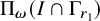
















































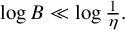




























Next, by the induction hypothesis at step r, we have that (3.11) and (3.12) hold for r. Also, by (Hii) at step r, if
$|\boldsymbol {x}-\boldsymbol {x}'|\leq (\tilde r+1)^{5C}\log M,$
 then (we hide the dependence on
$\xi , \xi ', \boldsymbol {\omega }, \boldsymbol {a}$
then (we hide the dependence on
$\xi , \xi ', \boldsymbol {\omega }, \boldsymbol {a}$
 )
)

If
$|\boldsymbol {x}-\boldsymbol {x}'|>(\tilde r+1)^{5C}\log M$
 , by (Hiii) at step r and Lemma 3.1, we have

The above estimates imply that for all
$\boldsymbol {x}, \boldsymbol {x}',$


Hence, combining (3.11)–(3.12) (at step r) and Lemma B.1, it follows that for any
$(\boldsymbol {\omega },\boldsymbol {a})\in \cup _{I\in \mathcal I_r}I$
 , we can replace
$\vec u^{(r-1)}$
, we can replace
$\vec u^{(r-1)}$
 in (3.11)–(3.12) with
$\vec u^{(r)}$
in (3.11)–(3.12) with
$\vec u^{(r)}$
 . That is to say,

and for
$|\boldsymbol {x}-\boldsymbol {x}'|>{\tilde r}^C,$


Assume
$|(\boldsymbol {\omega }, \boldsymbol {a})-(\boldsymbol {\omega }', \boldsymbol {a}')|\leq M^{-({\tilde r}+1)^{10C}}$
 . Similar to the above proof, we have for all
$\boldsymbol {x}, \boldsymbol {x}',$
. Similar to the above proof, we have for all
$\boldsymbol {x}, \boldsymbol {x}',$


Using Lemma B.1 again, we have that the estimates (3.21)–(3.22) and (3.15)–(3.16) (replacing
$\vec u^{(r_1)}$
 with
$\vec u^{(r)}$
with
$\vec u^{(r)}$
 ) allow
$O(M^{-({\tilde r}+1)^{10C}})$
) allow
$O(M^{-({\tilde r}+1)^{10C}})$
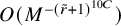 perturbation of
$(\boldsymbol {\omega }, \boldsymbol {a})$
perturbation of
$(\boldsymbol {\omega }, \boldsymbol {a})$
 . Combining conclusions in the above Case 1–Case 2 and the resolvent identity of [Reference He, Shi, Shi and YuanHSSY20] (cf. Lemma 3.6) gives a collection
$\mathcal {I}_{r+1}$
. Combining conclusions in the above Case 1–Case 2 and the resolvent identity of [Reference He, Shi, Shi and YuanHSSY20] (cf. Lemma 3.6) gives a collection
$\mathcal {I}_{r+1}$
 of intervals of size
$M^{-({\tilde r}+1)^{10C}}$
of intervals of size
$M^{-({\tilde r}+1)^{10C}}$
 so that for
$I\in \mathcal {I}_{r+1}$
so that for
$I\in \mathcal {I}_{r+1}$
 ,
,

which concludes (Hiv, c) at scale
$r+1.$
 We remark that in the above off-diagonal exponential decay estimates,
$c_{r+1}\geq c_r-(\log M)^C({\tilde r}+1)^{-C}$
We remark that in the above off-diagonal exponential decay estimates,
$c_{r+1}\geq c_r-(\log M)^C({\tilde r}+1)^{-C}$
 , which implies
$\inf _{r}c_r>0$
, which implies
$\inf _{r}c_r>0$
 . This explains why we need the sublinear-distance off-diagonal decay in LDT.
Finally, we have

Recalling that
$\boldsymbol {\omega }\to \boldsymbol {a}$
 is a
$C^1$
is a
$C^1$
 diffeomorphism and
$\det (\frac {\partial \boldsymbol {\omega }}{\partial \boldsymbol {a}})\sim \delta ^{b}$
diffeomorphism and
$\det (\frac {\partial \boldsymbol {\omega }}{\partial \boldsymbol {a}})\sim \delta ^{b}$
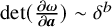 , we obtain since
$\varepsilon \leq \delta $
, we obtain since
$\varepsilon \leq \delta $
 that
that

which yields (Hiv, d) at step
$r+1.$ $\square $

Proof of Theorem 1.1
The proof of Theorem 1.1 is a direct corollary of the Inductive Theorem. We refer to [Reference Bourgain and WangBW08, Reference Liu and WangLW24] and Sections V and VI of [Reference Kachkovskiy, Liu and WangKLW24] for further details.
Appendix A Diophantine estimates
Below we provide Diophantine estimates when
$V(\boldsymbol {\theta })$
 is an (arbitrary) trigonometric polynomial. These estimates hold on a large set in
$(\boldsymbol {\alpha }, \boldsymbol {\theta })$
is an (arbitrary) trigonometric polynomial. These estimates hold on a large set in
$(\boldsymbol {\alpha }, \boldsymbol {\theta })$
 . The main idea is to utilize an appropriate generalized Wronskian approach. To our knowledge, these estimates did not appear to be known in the literature before. Given the relation between analytic functions (hence trigonometric polynomials) and generalized Wronskians, this approach also seems natural in hindsight.
To our knowledge, using transversality properties to make Diophantine approximations on manifolds was first developed by Pyartli [Reference PyartliPya69]. This method was later introduced into the study of KAM theory [Reference Xu, You and QiuXYQ97, Reference EliassonEli02, Reference BambusiBam03]. It turns out that this idea also plays a key role in the Craig-Wayne-Bourgain type argument used in the present paper. In addition, we can handle Diophantine estimates on general quasi-periodic polynomials on
$[0,1]^d$
 . The main difference between [Reference Xu, You and QiuXYQ97, Reference EliassonEli02, Reference BambusiBam03] and the present work is that we have no prior transversality estimate, which requires much additional effort.
Recall that

where
$\Gamma _K\subset [-K, K]^d\setminus \{\boldsymbol {0}\}$
 (
$K\in \mathbb {N}$
(
$K\in \mathbb {N}$
 ) is maximal so that

and

We also assume
$V(\boldsymbol {\theta })$
 is nondegenerate.
To handle
$\mu _{\boldsymbol {n}}=V(\boldsymbol {n}\boldsymbol {\alpha }+\boldsymbol {\theta })$
 , we need the following Łojasiewicz-type lemma.
Lemma A.1 (cf., for example, Lemma 4.2 in [Reference Jitomirskaya, Liu and ShiJLS20])
There exist some constants
$C_V>0, 0<c_V<1$
 depending only on V so that, for any
$\eta>0,$
depending only on V so that, for any
$\eta>0,$
 one has

Next, we fix

to be D (
$D\geq 2$
 ) distinct lattice points. We are mainly concerned with Diophantine estimates for

Throughout this Appendix, all constants
$C,c>0$
 are assumed to (depend only on
$d, K, D, V$
are assumed to (depend only on
$d, K, D, V$
 ) be independent of
$\boldsymbol {n}_s'$
) be independent of
$\boldsymbol {n}_s'$
 (
$1\leq s\leq D$
(
$1\leq s\leq D$
 ).
).
Our main result on the Diophantine estimates is
Theorem A.2. Let
$0<\eta <1$
 . We have for
$R=R_D=D\cdot (\#\Gamma _K)=D\frac {(2K+1)^d-1}{2}$
. We have for
$R=R_D=D\cdot (\#\Gamma _K)=D\frac {(2K+1)^d-1}{2}$
 ,
,

where
$C=C(d,K,D, V)>0$
 and
and

We also have for any
$\boldsymbol {k}'\in \mathbb Z^D\setminus \{\boldsymbol {0}\},$


Remark A.3. In contrast, if
$\boldsymbol {\omega }'$
 were a free parameter varying in
$[0,1]^D$
were a free parameter varying in
$[0,1]^D$
 , we would have

So the absence of independence of the coordinates of
$\boldsymbol {\omega }'$
 may lead to the corresponding measure bound (from
$1-O(\eta )$
may lead to the corresponding measure bound (from
$1-O(\eta )$
 to)
$1-O(\eta ^{\frac {1}{10dR^2}}).$
to)
$1-O(\eta ^{\frac {1}{10dR^2}}).$
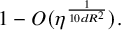
Recall that we have fixed in Theorem 1.1,

and for arbitrary
$\boldsymbol {n}$
 , we have
$\mu _{\boldsymbol {n}}=V(\boldsymbol {n}\boldsymbol {\alpha }+\boldsymbol {\theta }).$
, we have
$\mu _{\boldsymbol {n}}=V(\boldsymbol {n}\boldsymbol {\alpha }+\boldsymbol {\theta }).$

As a consequence of Lemma A.1 and Theorem A.2, we obtain
Corollary A.4. There exist some
$0<c_1=c_1(b,d,K,V)<\frac {1}{100b}, C_1=C_1(b,d, K, V)>1$
 such that, if
$0<\varepsilon +\delta \leq \delta _0(b,d,K,V,\max \limits _{1\leq \ell \leq b}|\boldsymbol {n}_\ell |)\ll 1$
such that, if
$0<\varepsilon +\delta \leq \delta _0(b,d,K,V,\max \limits _{1\leq \ell \leq b}|\boldsymbol {n}_\ell |)\ll 1$
 , then there is some
$\mathcal M \subset [0, 1]^{2d}$
, then there is some
$\mathcal M \subset [0, 1]^{2d}$
 satisfying

so that the following properties hold true for
$(\boldsymbol {\alpha }, \boldsymbol {\theta })\in \mathcal M$
 and
$L_{\varepsilon ,\delta }=100(\varepsilon +\delta )^{-c_1}$
and
$L_{\varepsilon ,\delta }=100(\varepsilon +\delta )^{-c_1}$
 .
.
-
(i). For any $\boldsymbol {n}\neq \boldsymbol {n}'$
satisfying
$|\boldsymbol {n}|, |\boldsymbol {n}'|\leq L_{\varepsilon ,\delta }$
, $$ \begin{align*}|\mu_{\boldsymbol{n}}-\mu_{\boldsymbol{n}'}|\geq (\varepsilon+\delta)^{\frac{1}{8b}}.\end{align*} $$
-
(ii). For any $\boldsymbol {k}\in \mathbb Z^b$
satisfying
$0<|\boldsymbol {k}|\leq 2L_{\varepsilon ,\delta },$
$$ \begin{align*}|\boldsymbol{k}\cdot \boldsymbol{\omega}^{(0)}|\geq (\varepsilon+\delta)^{\frac{1}{8b}}.\end{align*} $$
-
(iii). For any $\log \frac {1}{\varepsilon +\delta }\leq L\leq L_{\varepsilon ,\delta }$
and all
$(\boldsymbol {k},\boldsymbol {n})\in \Lambda _{L}\setminus \mathcal S,$
$$ \begin{align*}\min_{\xi=\pm1}|\xi \boldsymbol{k}\cdot \boldsymbol{\omega}^{(0)}+\mu_{\boldsymbol{n}}|\geq L^{-C_1}.\end{align*} $$
-
(iv). For any $(\boldsymbol {k}, \boldsymbol {n}, \boldsymbol {n}')\in \mathbb Z^b\times \mathbb Z^d\times \mathbb Z^d$
satisfying
$|\boldsymbol {k}|\leq 2L_{\varepsilon ,\delta }, |(\boldsymbol {n}, \boldsymbol {n}')|\leq L_{\varepsilon ,\delta }$
and
$\boldsymbol {k}\cdot \boldsymbol {\omega }^{(0)}+ \mu _{\boldsymbol {n}}-\mu _{\boldsymbol {n}'}\not \equiv 0,$
$$ \begin{align*}|\boldsymbol{k}\cdot \boldsymbol{\omega}^{(0)}+\mu_{\boldsymbol{n}}-\mu_{\boldsymbol{n}'}|\geq (\varepsilon+\delta)^{\frac{1}{8b}}.\end{align*} $$













Proof. It suffices to apply Lemma A.1 (i.e.,
$D=1$
 ) and Theorem A.2 with
$\eta =(\varepsilon +\delta )^{\frac {1}{8b}}, L^{-C_1}$
) and Theorem A.2 with
$\eta =(\varepsilon +\delta )^{\frac {1}{8b}}, L^{-C_1}$
 and
$D=2, b+1, b+2$
and
$D=2, b+1, b+2$
 . Without loss of generality, we only deal with (iii) and (iv) since (i) and (ii) can be handled similarly.
(iii). Denote by
$\mathcal {M}_{\mathrm {iii}}$
 the set of
$(\boldsymbol {\alpha }, \boldsymbol {\theta })\in [0,1]^{2d}$
the set of
$(\boldsymbol {\alpha }, \boldsymbol {\theta })\in [0,1]^{2d}$
 so that the conclusion of (iii) holds true.
For the case of
$\boldsymbol {k}=\boldsymbol {0}$
 , applying Lemma A.1 yields for all
$\boldsymbol {\alpha }\in [0,1]^d,$
, applying Lemma A.1 yields for all
$\boldsymbol {\alpha }\in [0,1]^d,$


where in the last inequality we assume
$0<\varepsilon +\delta \leq \delta _0(V,d)\ll 1.$

For the case of
$\boldsymbol {k}\neq \boldsymbol {0}$
 and
$\boldsymbol {n}\notin \{\boldsymbol {n}_1,\cdots , \boldsymbol {n}_b\}$
and
$\boldsymbol {n}\notin \{\boldsymbol {n}_1,\cdots , \boldsymbol {n}_b\}$
 , we apply Theorem A.2 with
$D=b+1, \eta =L^{-C_1}$
, we apply Theorem A.2 with
$D=b+1, \eta =L^{-C_1}$
 and
$\boldsymbol {k}'=(\pm \boldsymbol {k}, 1)$
and
$\boldsymbol {k}'=(\pm \boldsymbol {k}, 1)$
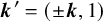 to get for

the following

where in the last inequality we assume
$0<\varepsilon +\delta \leq \delta _0(b,d, K, V,\max \limits _{1\leq \ell \leq b}|\boldsymbol {n}_\ell |)\ll 1.$
 The case of
$\boldsymbol {k}\neq \boldsymbol {0}$
The case of
$\boldsymbol {k}\neq \boldsymbol {0}$
 and
$\boldsymbol {n}\in \{\boldsymbol {n}_1,\cdots , \boldsymbol {n}_b\}$
and
$\boldsymbol {n}\in \{\boldsymbol {n}_1,\cdots , \boldsymbol {n}_b\}$
 can be handled similarly and we omit the details. Since there are only 3 cases to deal with,
$C_1=C_1(b,d,K,V)>0$
can be handled similarly and we omit the details. Since there are only 3 cases to deal with,
$C_1=C_1(b,d,K,V)>0$
 can be well-defined.
By combining all the above estimates, we obtain the desired measure bound on
$\mathcal {M}_{\mathrm {iii}}$
 , namely,

(iv). If
$x,y\in \mathbb R$
 , we denote
$x\wedge y=\min \{x, y\}$
, we denote
$x\wedge y=\min \{x, y\}$
 and
$x\vee y=\max \{x, y\}$
and
$x\vee y=\max \{x, y\}$
 . Denote by
$\mathcal {M}_{\mathrm {iv}}$
. Denote by
$\mathcal {M}_{\mathrm {iv}}$
 the set of
$(\boldsymbol {\alpha }, \boldsymbol {\theta })\in [0,1]^{2d}$
the set of
$(\boldsymbol {\alpha }, \boldsymbol {\theta })\in [0,1]^{2d}$
 so that the conclusion of (iv) holds true. First we consider the case of
$(\boldsymbol {k}, \boldsymbol {n}, \boldsymbol {n}')\in \mathcal T_1$
so that the conclusion of (iv) holds true. First we consider the case of
$(\boldsymbol {k}, \boldsymbol {n}, \boldsymbol {n}')\in \mathcal T_1$
 with
$\mathcal T_1$
with
$\mathcal T_1$
 the set of all
$(\boldsymbol {k}, \boldsymbol {n}, \boldsymbol {n}')$
the set of all
$(\boldsymbol {k}, \boldsymbol {n}, \boldsymbol {n}')$
 satisfying:
$0<|\boldsymbol {k}|\leq 2L_{\varepsilon ,\delta }, |(\boldsymbol {n}, \boldsymbol {n}')|\leq L_{\varepsilon ,\delta }$
satisfying:
$0<|\boldsymbol {k}|\leq 2L_{\varepsilon ,\delta }, |(\boldsymbol {n}, \boldsymbol {n}')|\leq L_{\varepsilon ,\delta }$
 ,
$ \boldsymbol {n}\neq \boldsymbol {n}'$
,
$ \boldsymbol {n}\neq \boldsymbol {n}'$
 ,
$\mathrm {both}\ \boldsymbol {n}\ \mathrm {and}\ \boldsymbol {n}'\ \notin \{\boldsymbol {n}_1,\cdots , \boldsymbol {n}_b\}.$
,
$\mathrm {both}\ \boldsymbol {n}\ \mathrm {and}\ \boldsymbol {n}'\ \notin \{\boldsymbol {n}_1,\cdots , \boldsymbol {n}_b\}.$
 We let

So we can apply Theorem A.2 with
$D=b+2,\eta =(\varepsilon +\delta )^{\frac {1}{8b}}$
 and
$\boldsymbol {k}'=(\boldsymbol {k}, 1, -1)$
and
$\boldsymbol {k}'=(\boldsymbol {k}, 1, -1)$
 to get

where in the last inequality we assume
$0<\varepsilon +\delta \leq \delta _0(b,d, K, V,\max \limits _{1\leq \ell \leq b}|\boldsymbol {n}_\ell |)\ll 1.$

Next, we consider the case of
$(\boldsymbol {k}, \boldsymbol {n},\boldsymbol {n}')$
 with
$\boldsymbol {k}\cdot \boldsymbol {\omega }^{(0)}+\mu _{\boldsymbol {n}}\equiv 0$
with
$\boldsymbol {k}\cdot \boldsymbol {\omega }^{(0)}+\mu _{\boldsymbol {n}}\equiv 0$
 . In this case, applying Lemma A.1 yields for all
$\boldsymbol {\alpha }\in [0,1]^d,$
. In this case, applying Lemma A.1 yields for all
$\boldsymbol {\alpha }\in [0,1]^d,$


where in the last inequality we assume
$0<\varepsilon +\delta \leq \delta _0(b,d,V)\ll 1.$
 Other cases are easier to handle, and we omit the details. By taking into account all the above estimates, we have

Note that since there are only finitely many (say, at most 10) cases to deal with,
$c_1=c_1(b,d, K, V)>0$
 can be well-defined.
A.1 Some useful lemmas
In this section, we will introduce some useful lemmas.
Lemma A.5 [Reference Kleinbock and MargulisKM98]
Let
$I\subset \mathbb R$
 be an interval of finite length (i.e.,
$0<|I|<\infty $
be an interval of finite length (i.e.,
$0<|I|<\infty $
 ) and
$k\geq 1.$
) and
$k\geq 1.$
 If
$f\in C^{k}(I;\mathbb R)$
If
$f\in C^{k}(I;\mathbb R)$
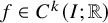 satisfies

then for all
$\varepsilon>0,$


where
$\zeta _k=k(k+1)((k+1)!)^{\frac 1k}.$

Proof. The following proof is taken from Kleinbock-Margulis [Reference Kleinbock and MargulisKM98].
From (A.2) and Rolle’s theorem, the equation
$\frac {d}{dx}f(x)=0$
 has at most k zeros on I. This then implies that the set
$\{x\in I:\ |f(x)|\leq \varepsilon \}$
has at most k zeros on I. This then implies that the set
$\{x\in I:\ |f(x)|\leq \varepsilon \}$
 consists of at most
$k+1$
consists of at most
$k+1$
 intervals. Denote by
$I_1$
intervals. Denote by
$I_1$
 one of those subintervals having maximal length. So we get

To prove (A.3), it remains to estimate
$|I_1|>0$
 . We divide
$I_1$
. We divide
$I_1$
 into k equal parts by points
$x_1,\cdots , x_{k+1}.$
into k equal parts by points
$x_1,\cdots , x_{k+1}.$
 Let
$P(x)$
Let
$P(x)$
 be the Lagrange polynomial of f on points
$x_1,\cdots , x_{k+1},$
be the Lagrange polynomial of f on points
$x_1,\cdots , x_{k+1},$
 namely,

By applying Rolle’s theorem k times and since
$f(x_i)=P(x_i)$
 (
$1\leq i \leq k+1$
(
$1\leq i \leq k+1$
 ), we can find
$x_0\in I_1$
), we can find
$x_0\in I_1$
 so that

which together with (A.2) yields

This implies

We have finished the proof.
In the following, we turn to the analysis of multi-variable functions. We first introduce the notations.
-
○ For any ${\boldsymbol {x}}=(x_1,\cdots ,x_d)$
and any
$d\geq 1$
, let $$ \begin{align*}|{\boldsymbol{x}}|_2=\sqrt{\sum_{i=1}^d|x_i|^2},\ |\boldsymbol{x}|_1=\sum_{i=1}^d|x_i|.\end{align*} $$
-
○ Let $\boldsymbol {a}=(a_1,\cdots ,a_d), \boldsymbol {b}=(b_1,\cdots ,b_d)$
. Define the d-dimensional interval to be (A.4) $$ \begin{align} I=I_{\boldsymbol{a}, \boldsymbol{b}}=\prod_{i=1}^d[a_i,b_i]\subset\mathbb R^d. \end{align} $$
$$ \begin{align*}|\boldsymbol{a}\vee \boldsymbol{b}|=\sum_{i=1}^d \max(|a_i|, |b_i|).\end{align*} $$
-
○ For ${\boldsymbol {\beta }}=(\beta _1,\cdots ,\beta _d)\in \mathbb R^d\setminus \{\boldsymbol {0}\}$
, define $$ \begin{align*} d_{\boldsymbol{\beta}}:=\sum_{i=1}^d\beta_i{\partial}_i,\ \partial_i:=\frac{\partial}{\partial x_i}. \end{align*} $$We also write for $\ell \geq 1, $
$$ \begin{align*}d_{\boldsymbol{\beta}}^\ell=d_{\boldsymbol{\beta}}\cdots d_{\boldsymbol{\beta}}\ (\ell-\mathrm{times}).\end{align*} $$Denote
$$ \begin{align*}\nabla=(\partial_1,\cdots,\partial_d).\end{align*} $$
-
○ For a multi-index ${\boldsymbol {\gamma }}=(\gamma _1,\cdots ,\gamma _d)\in \mathbb {N}^d$
, denote $$ \begin{align*} |\boldsymbol{\gamma}|=\sum_{i=1}^d\gamma_i,\ \partial^{\boldsymbol{\gamma}}=\partial^{\gamma_1}_1\cdots\partial^{\gamma_d}_d. \end{align*} $$











We have
Lemma A.6. Fix
$k\in \mathbb {N}$
 . Let
$I=I_{\boldsymbol {a}, \boldsymbol {b}}\subset \mathbb R^d$
. Let
$I=I_{\boldsymbol {a}, \boldsymbol {b}}\subset \mathbb R^d$
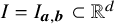 be defined by (A.4). Assume that the function
$f\in C^{k+1}(I;\mathbb R)$
be defined by (A.4). Assume that the function
$f\in C^{k+1}(I;\mathbb R)$
 satisfies for some
$A>0,$
satisfies for some
$A>0,$


Let

Then for
$0<\varepsilon <1,$


where
$C=C(\boldsymbol {\beta }, k,d)>0$
 depends only on
$\boldsymbol {\beta }, k,d $
depends only on
$\boldsymbol {\beta }, k,d $
 (but not on f).
Remark A.7. If f is a polynomial on
$\mathbb R^d$
 , [Reference Carbery and WrightCW01] proved some strong distributional inequalities, which may directly imply (A.6). However, in the present case, we have a weak transversality condition (A.5). So we would like to give an elementary proof applying for more general functions (cf. [Reference Liu, Shi and ZhangLSZ25] for an application), which also produces an upper bound in the estimate (A.6) with the explicit dependence on
$\|f\|_{k+1}$
, [Reference Carbery and WrightCW01] proved some strong distributional inequalities, which may directly imply (A.6). However, in the present case, we have a weak transversality condition (A.5). So we would like to give an elementary proof applying for more general functions (cf. [Reference Liu, Shi and ZhangLSZ25] for an application), which also produces an upper bound in the estimate (A.6) with the explicit dependence on
$\|f\|_{k+1}$
 .
.
Proof. The proof can be divided into two steps:
Step 1. Assume that for some
$1\leq k_1\leq k$
 and interval
$I_1=\prod _{i=1}^d[h_i,m_i],$
and interval
$I_1=\prod _{i=1}^d[h_i,m_i],$


We will combine Lemma A.5 and Fubini’s theorem to deal with the measure estimate. Let
$\boldsymbol {e}_1=\frac {\boldsymbol {\beta }}{|\boldsymbol {\beta }|_2}$
 and choose a normalized orthogonal basis
$\boldsymbol {e}_2,\cdots , \boldsymbol {e}_d\in \mathbb R^d$
and choose a normalized orthogonal basis
$\boldsymbol {e}_2,\cdots , \boldsymbol {e}_d\in \mathbb R^d$
 of
of

We can then define the coordinate transform:

via

So the Jacobian satisfies

Define

and denote by
$\chi _{(\cdot )}$
 the indicator function. We have

We proceed to control
$\boldsymbol {\varphi }^{-1}(I_1)$
 . From
$\boldsymbol {x}=s\boldsymbol {e}_1+\sum _{i=2}^d y_i\boldsymbol {e}_i\in I_1$
. From
$\boldsymbol {x}=s\boldsymbol {e}_1+\sum _{i=2}^d y_i\boldsymbol {e}_i\in I_1$
 , we obtain

Similarly, we also have
$y_i\in [-|\boldsymbol {h}\vee \boldsymbol {m}|, |\boldsymbol {h}\vee \boldsymbol {m}|]$
 for
$2\leq i\leq d,$
for
$2\leq i\leq d,$
 which yields
$\boldsymbol {\varphi }^{-1}(I_1)\subset [-|\boldsymbol {h}\vee \boldsymbol {m}|, |\boldsymbol {h}\vee \boldsymbol {m}|]^d$
which yields
$\boldsymbol {\varphi }^{-1}(I_1)\subset [-|\boldsymbol {h}\vee \boldsymbol {m}|, |\boldsymbol {h}\vee \boldsymbol {m}|]^d$
 . We define

and, define for
$\boldsymbol {y}\in \Pi _1\boldsymbol {\varphi }^{-1}(I_1), $
 the interval
$I_{\boldsymbol {y}}=\{s\in \mathbb R:\ (s,\boldsymbol {y})\in \boldsymbol {\varphi }^{-1}(I_1)\}$
the interval
$I_{\boldsymbol {y}}=\{s\in \mathbb R:\ (s,\boldsymbol {y})\in \boldsymbol {\varphi }^{-1}(I_1)\}$
 of finite length. Applying Fubini’s theorem together with (A.8) implies that

For fixed
$\boldsymbol {y}\in \Pi _1\boldsymbol {\varphi }^{-1}(I_1)$
 , we get

Denote
$g(s)=f(s\boldsymbol {e}_1+\sum _{i=2}^dy_i\boldsymbol {e}_i)$
 . From (A.7), we have for all
$s\in I_{\boldsymbol {y}},$
. From (A.7), we have for all
$s\in I_{\boldsymbol {y}},$


So applying Lemma A.5 yields

Step 2. We deal with the general case in this step. So we first divide each one-dimensional interval
$[a_i,b_i]$
 into N (will be specified below) equal subintervals
$I_{i,j_i}$
into N (will be specified below) equal subintervals
$I_{i,j_i}$
 (
$1\leq j_i\leq N$
(
$1\leq j_i\leq N$
 ). This then induces a decomposition of I, namely,

We will apply the argument proved in Step 1 on each
$I_{\boldsymbol {J}}$
 . For this purpose, we fix
$I_{\boldsymbol {J}}$
. For this purpose, we fix
$I_{\boldsymbol {J}}$
 . For any
$\boldsymbol {x},\boldsymbol {y}\in I_{\boldsymbol {J}}$
. For any
$\boldsymbol {x},\boldsymbol {y}\in I_{\boldsymbol {J}}$
 , we have

Fixing any
$\boldsymbol {x}_0\in I_{\boldsymbol {J}}$
 , we get from the assumption (A.5) that there exists
$1\leq k_1\leq k$
, we get from the assumption (A.5) that there exists
$1\leq k_1\leq k$
 with
with

As a result, for any
$\boldsymbol {x}\in I_{\boldsymbol {J}}$
 , we obtain

where

In fact,
$L_{\boldsymbol {\beta }, d}$
 is derived from

From (A.10), we can set

so that

where
$[x]$
 denotes the integer part of
$x\in \mathbb R.$
denotes the integer part of
$x\in \mathbb R.$
 Thus applying (A.9) yields (since
$I_J\subset I, 0<\varepsilon <1$
Thus applying (A.9) yields (since
$I_J\subset I, 0<\varepsilon <1$
 )
)

Collecting all
$I_{\boldsymbol {J}}$
 leads to,

We have proven (A.6).
Finally, we introduce a key lemma (cf. Proposition in Appendix B, [Reference Benettin, Galgani and GiorgilliBGG85] for a more precise form) on determinant estimates.
Lemma A.8. Let
$\boldsymbol {v}^{(1)},\cdots , \boldsymbol {v}^{(r)}\in \mathbb R^r$
 be r linearly independent vectors with
$|\boldsymbol {v}^{(\ell )}|_1\leq M$
be r linearly independent vectors with
$|\boldsymbol {v}^{(\ell )}|_1\leq M$
 for
$1\leq \ell \leq r.$
for
$1\leq \ell \leq r.$
 Then for any
$\boldsymbol {w}\in \mathbb R^r$
Then for any
$\boldsymbol {w}\in \mathbb R^r$
 , we have

Proof. For completeness, we give a proof based on Cramer’s rule and the Hadamard’s inequality. We assume
$\boldsymbol {v}^{(\ell )}$
 is the row vector in
$\mathbb R^r$
is the row vector in
$\mathbb R^r$
 (
$1\leq \ell \leq r$
(
$1\leq \ell \leq r$
 ). Denote by
$X=[\boldsymbol {v}^{(1)},\cdots , \boldsymbol {v}^{(r)}]$
). Denote by
$X=[\boldsymbol {v}^{(1)},\cdots , \boldsymbol {v}^{(r)}]$
 the
$r\times r $
the
$r\times r $
 matrix and consider the equation

By the Cramer’s rule, we obtain

where
$X^*=[\tilde v_{ij}]_{1\leq i,j\leq r}$
 denotes the adjugate matrix of X. As a result, we get

It remains to bound
$\max _{1\leq i,j\leq r}|\tilde v_{ij}|,$
 which will be completed by using the Hadamard’s inequality. In fact, we have

This finishes the proof.
A.2 Proof of Theorem A.2
In this section, we prove Theorem A.2.
Proof of Theorem A.2
Recall that

where

Denote
$\boldsymbol {\xi }=(\boldsymbol {\beta }, \boldsymbol {q})$
 for
$\boldsymbol {\beta }, \boldsymbol {q}\in [0,1]^d$
for
$\boldsymbol {\beta }, \boldsymbol {q}\in [0,1]^d$
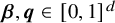 . Write also

and accordingly
$d_{\boldsymbol {\xi }}^\ell $
 for
$\ell \geq 1.$
for
$\ell \geq 1.$

A key observation is that for all
$j\geq 1$
 and
$\boldsymbol {\ell } \in \Gamma _K$
and
$\boldsymbol {\ell } \in \Gamma _K$
 ,
,

This motivates us to consider the Wronskian

which is a
$R\times R$
 real matrix. Direct computations show

where
$W_1$
 is a Vandermonde matrix with

Then the proof can be divided into three steps:
Step 1. Prior conditions on
$(\boldsymbol {\alpha } , \boldsymbol {\theta })$

We aim to get a lower bound for (A.11), which requires the prior restrictions on
$\boldsymbol {\alpha }, \boldsymbol {\theta }.$
 Let
$\|x\|_{\mathbb {T}/2}=\mathrm {dist} (x, \mathbb Z/2)$
Let
$\|x\|_{\mathbb {T}/2}=\mathrm {dist} (x, \mathbb Z/2)$
 . From

we can define for
$\delta>0$
 the resonant set (of
$\boldsymbol {\alpha }, \boldsymbol {\theta }$
the resonant set (of
$\boldsymbol {\alpha }, \boldsymbol {\theta }$
 )
)

Denote
$L=\max \limits _{1\leq s\leq D} K |\boldsymbol {n}_s'|$
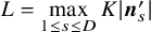 . We have
Lemma A.9. Let
$0<\delta <1$
 . Then
$S_\delta $
. Then
$S_\delta $
 can be covered by
$C L^{2d-1}\delta ^{-2d+1}$
can be covered by
$C L^{2d-1}\delta ^{-2d+1}$
 intervals of side length
$\leq \delta ,$
intervals of side length
$\leq \delta ,$
 where
$C=C(d,R)>0.$
where
$C=C(d,R)>0.$

Proof. It suffices to cover for each
$\boldsymbol {n}_s^{\prime }, \boldsymbol {\ell }$
 the set

with
$C(d) L^{2d-1} \delta ^{-2d+1}$
 intervals of side length
$\leq \delta $
intervals of side length
$\leq \delta $
 since the total number of all
$\boldsymbol {n}_s^{\prime }, \boldsymbol {\ell }$
since the total number of all
$\boldsymbol {n}_s^{\prime }, \boldsymbol {\ell }$
 is at most
$R.$
is at most
$R.$
 Since
$|\boldsymbol {\ell }|>0,$
Since
$|\boldsymbol {\ell }|>0,$
 we may assume
$\ell _1\neq 0$
we may assume
$\ell _1\neq 0$
 without loss of generality. For any
$\boldsymbol {x}=(x_1,\cdots , x_d),$
without loss of generality. For any
$\boldsymbol {x}=(x_1,\cdots , x_d),$
 write
$\boldsymbol {x}=(x_1, \boldsymbol {x}^c_1)$
write
$\boldsymbol {x}=(x_1, \boldsymbol {x}^c_1)$
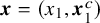 . So we can divide
$[0,1]^d\times [0,1]^{d-1}\ni (\boldsymbol {\alpha }, \boldsymbol {\theta }_1^c)$
. So we can divide
$[0,1]^d\times [0,1]^{d-1}\ni (\boldsymbol {\alpha }, \boldsymbol {\theta }_1^c)$
 into
$C_1=[100L\delta ^{-1}]^{2d-1}$
into
$C_1=[100L\delta ^{-1}]^{2d-1}$
 cubes
$\boldsymbol {C}_i$
cubes
$\boldsymbol {C}_i$
 (
$1\leq i\leq C_1$
(
$1\leq i\leq C_1$
 ) with disjoint exteriors of the same side length
$\leq \frac {\delta }{ L}$
) with disjoint exteriors of the same side length
$\leq \frac {\delta }{ L}$
 . Denote by
$ (\boldsymbol {\alpha }_i, \boldsymbol {\theta }^c(i))\in [0,1]^{d}\times [0,1]^{d-1}$
. Denote by
$ (\boldsymbol {\alpha }_i, \boldsymbol {\theta }^c(i))\in [0,1]^{d}\times [0,1]^{d-1}$
 (
$1\leq i\leq C_1$
(
$1\leq i\leq C_1$
 ) the centers of those cubes. We further define

We first claim that
$S_{\boldsymbol {n}_s^{\prime }, \boldsymbol {\ell }} \subset I_{\boldsymbol {n}_s^{\prime }, \boldsymbol {\ell }}.$
 Let
$(\boldsymbol {\alpha }, \boldsymbol {\theta })\in S_{\boldsymbol {n}_s', \boldsymbol {\ell }}$
Let
$(\boldsymbol {\alpha }, \boldsymbol {\theta })\in S_{\boldsymbol {n}_s', \boldsymbol {\ell }}$
 . Then by the definition (of
$S_{\boldsymbol {n}_s^{\prime }, \boldsymbol {\ell }}$
. Then by the definition (of
$S_{\boldsymbol {n}_s^{\prime }, \boldsymbol {\ell }}$
 ), we have

Since
$\boldsymbol {C}_i$
 (
$1\leq i\leq C_1$
(
$1\leq i\leq C_1$
 ) covers
$[0,1]^{2d-1}$
) covers
$[0,1]^{2d-1}$
 , there is
$1 \leq i_0\leq C_1$
, there is
$1 \leq i_0\leq C_1$
 so that
$(\boldsymbol {\alpha }, \boldsymbol {\theta }_1^c)\in \boldsymbol {C}_{i_0}$
so that
$(\boldsymbol {\alpha }, \boldsymbol {\theta }_1^c)\in \boldsymbol {C}_{i_0}$
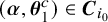 , namely,
$|\boldsymbol {\alpha }-\boldsymbol {\alpha }_{i_0}|+|\boldsymbol {\theta }_1^c-\boldsymbol {\theta }^c(i_0)|\leq \frac {\delta }{ 2L}.$
, namely,
$|\boldsymbol {\alpha }-\boldsymbol {\alpha }_{i_0}|+|\boldsymbol {\theta }_1^c-\boldsymbol {\theta }^c(i_0)|\leq \frac {\delta }{ 2L}.$
 This implies that

The claim is proved. So it remains to cover each
$J_i$
 with intervals of side length
$\leq \delta $
with intervals of side length
$\leq \delta $
 . This can be accomplished by the fact that the set
$\{\theta _1\in [0,1]:\ \|\ell _1\theta _1+x\|_{\mathbb {T}/2}\leq 2\delta \}$
. This can be accomplished by the fact that the set
$\{\theta _1\in [0,1]:\ \|\ell _1\theta _1+x\|_{\mathbb {T}/2}\leq 2\delta \}$
 (
$x\in \mathbb R$
(
$x\in \mathbb R$
 ) consists of
$r\sim |\ell _1|$
) consists of
$r\sim |\ell _1|$
 one-dimensional intervals of length
$2\delta /|\ell _1|$
one-dimensional intervals of length
$2\delta /|\ell _1|$
 .
.
We have finished the proof.
Given
$0<\delta <1/10,$
 we divide
$[0,1]$
we divide
$[0,1]$
 into
$N=[\delta ^{-2}]+1$
into
$N=[\delta ^{-2}]+1$
 intervals of equal length
$\frac 1N\sim \delta ^2$
intervals of equal length
$\frac 1N\sim \delta ^2$
 . This then induces a partition of
$[0,1]^{2d}$
. This then induces a partition of
$[0,1]^{2d}$
 into cubes of equal side length
$1/N$
into cubes of equal side length
$1/N$
 . We denote by
$\Lambda _{1/N}(\boldsymbol {x}_i) $
. We denote by
$\Lambda _{1/N}(\boldsymbol {x}_i) $
 (
$1\leq i\leq N^{2d}$
(
$1\leq i\leq N^{2d}$
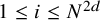 ) all these cubes. We have
Lemma A.10. Let
$0<\delta <1/10$
 and let
$S_\delta $
and let
$S_\delta $
 be defined by (A.13). Then we have for
$N=[\delta ^{-2}]+1$
be defined by (A.13). Then we have for
$N=[\delta ^{-2}]+1$
 ,
,

In particular, we have

Proof. Let
$ \boldsymbol {C}_i$
 be given as in the proof of Lemma A.9. Then
$S_\delta \subset \cup _{1\leq i\leq C(d,R)L^{2d-1}\delta ^{-2d+1}}\boldsymbol {C}_i$
be given as in the proof of Lemma A.9. Then
$S_\delta \subset \cup _{1\leq i\leq C(d,R)L^{2d-1}\delta ^{-2d+1}}\boldsymbol {C}_i$
 . So it suffices to bound

Note that if
$\Lambda _{1/N}(\boldsymbol {x}_i)\cap \boldsymbol {C}_j\neq \emptyset $
 , then

where
$ \boldsymbol {C}_j^{\prime }$
 is also an interval containing
$\boldsymbol {C}_j$
is also an interval containing
$\boldsymbol {C}_j$
 and satisfying

with
$\partial $
 the boundary. Regarding the disjointness (of the exterior) of
$\Lambda _{1/N}(\boldsymbol {x}_i)$
the boundary. Regarding the disjointness (of the exterior) of
$\Lambda _{1/N}(\boldsymbol {x}_i)$
 for different i, we must have

This implies the bound (A.14). Then the measure bound follows directly from (A.15).
From this lemma, we get immediately that
Lemma A.11. Let
$0<\delta <1/10$
 and define
$N=[\delta ^{-2}]+1$
and define
$N=[\delta ^{-2}]+1$
 . Then there is a collection of cubes
$\Lambda _{1/N}(\boldsymbol {x}_i) \subset [0,1]^{d+d}$
. Then there is a collection of cubes
$\Lambda _{1/N}(\boldsymbol {x}_i) \subset [0,1]^{d+d}$
 (
$1\leq i\leq N_1$
(
$1\leq i\leq N_1$
 ) with disjoint exteriors so that

and if
$(\boldsymbol {\alpha },\boldsymbol {\theta })\in \cup _{1\leq i\leq N_1}\Lambda _{1/N}(\boldsymbol {x}_i),$
 then
then

Step 2. Conditions on
$(\boldsymbol {\beta }, \boldsymbol {q})$

Next we impose conditions on
$(\boldsymbol {\beta }, \boldsymbol {q})$
 .
.
Lemma A.12. Let
$\epsilon \in (0,1)$
 and
$\boldsymbol {B}\subset [0,1]^d\times [0,1]^d $
and
$\boldsymbol {B}\subset [0,1]^d\times [0,1]^d $
 be the set of
$\boldsymbol {\xi }=(\boldsymbol {\beta }, \boldsymbol {q})$
be the set of
$\boldsymbol {\xi }=(\boldsymbol {\beta }, \boldsymbol {q})$
 satisfying

Then

Moreover, for
$\boldsymbol {\xi }\in \boldsymbol {B},$
 we have

Proof. The proof is based on Fubini’s theorem, (A.1) and the assumption on
$\boldsymbol {n}_s^{\prime }$
 (
$1\leq s\leq D$
(
$1\leq s\leq D$
 ). Actually, in all cases we have

which combined with
$s\leq D$
 and
$\boldsymbol {\ell }\in \Gamma _K$
and
$\boldsymbol {\ell }\in \Gamma _K$
 leads to the excision of
$(\boldsymbol {\beta }, \boldsymbol {q})$
leads to the excision of
$(\boldsymbol {\beta }, \boldsymbol {q})$
 in a set of measure
$O(\sqrt {\epsilon })$
in a set of measure
$O(\sqrt {\epsilon })$
 .
.
Step 3. Usage of the Lemma A.8
Now combining Lemma A.11 and Lemma A.12 (we set
$\epsilon =10^{-2}R^{-4}$
 ) leads to
Lemma A.13. Let
$0<\delta <1/10$
 and define
$N=[\delta ^{-2}]+1$
and define
$N=[\delta ^{-2}]+1$
 . Then there is a collection of cubes
$\Lambda _{1/N}(\boldsymbol {x}_i) \subset [0,1]^{2d}$
. Then there is a collection of cubes
$\Lambda _{1/N}(\boldsymbol {x}_i) \subset [0,1]^{2d}$
 (
$1\leq i\leq N_1$
(
$1\leq i\leq N_1$
 for some
$N_1>1$
for some
$N_1>1$
 ) with disjoint exteriors, and a set
$\boldsymbol {B}\subset [0,1]^{2d}$
) with disjoint exteriors, and a set
$\boldsymbol {B}\subset [0,1]^{2d}$
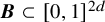 so that

Moreover, if
$(\boldsymbol {\alpha },\boldsymbol {\theta })\in \cup _{1\leq i\leq N_1}\Lambda _{1/N}(\boldsymbol {x}_i) $
 and
$\boldsymbol {\xi }\in \boldsymbol {B},$
and
$\boldsymbol {\xi }\in \boldsymbol {B},$
 then
then

We are ready to conclude the proof of Theorem A.2. Fix
$\boldsymbol {\xi }\in \boldsymbol {B}$
 and a
$1/N\sim \delta ^2$
and a
$1/N\sim \delta ^2$
 -cube
$\Lambda _i=\Lambda _{1/N}(\boldsymbol {x}_i)\subset [0,1]^{2d}$
-cube
$\Lambda _i=\Lambda _{1/N}(\boldsymbol {x}_i)\subset [0,1]^{2d}$
 in Lemma A.13. We will deal with
$(\boldsymbol {\alpha }, \boldsymbol {\theta })\in \Lambda _i.$
in Lemma A.13. We will deal with
$(\boldsymbol {\alpha }, \boldsymbol {\theta })\in \Lambda _i.$
 Denote for
$\boldsymbol {k}^{\prime }\in \mathbb Z^D\setminus \{\boldsymbol {0}\}$
Denote for
$\boldsymbol {k}^{\prime }\in \mathbb Z^D\setminus \{\boldsymbol {0}\}$
 ,
,

Direct computations show that for
$\boldsymbol {\xi }=(\boldsymbol {\beta }, \boldsymbol {q}),$


We have by Lemma A.13 and Lemma A.8 that

where
$c=c(d,R, V)>0.$

It suffices to apply Lemma A.6 by letting
$k=2R$
 . The transversality condition has been verified by (A.16). For
$f(\boldsymbol {\alpha }, \boldsymbol {\theta })=\boldsymbol {k}'\cdot \boldsymbol {\omega }'$
. The transversality condition has been verified by (A.16). For
$f(\boldsymbol {\alpha }, \boldsymbol {\theta })=\boldsymbol {k}'\cdot \boldsymbol {\omega }'$
 , we have

So using Lemma A.6 by setting
$\varepsilon =\frac {\eta }{|\boldsymbol {k}^{\prime }|^{4R^2}}$
 leads to

Together with Lemma A.13 this yields

This proves Theorem A.2.
Appendix B Some important lemmas
Let
$M_2(\mathbb C)$
 denote the Banach algebra of all
$(2\times 2)$
denote the Banach algebra of all
$(2\times 2)$
 -complex matrices equipped with the standard operator norm. Since the index
$\xi \in \{+,-\}$
-complex matrices equipped with the standard operator norm. Since the index
$\xi \in \{+,-\}$
 , we can identify the matrix from
$\mathbb Z^{b+d}_{\mathrm {pm}}$
, we can identify the matrix from
$\mathbb Z^{b+d}_{\mathrm {pm}}$
 to
$\mathbb C$
to
$\mathbb C$
 with that from
$\mathbb Z^{b+d}$
with that from
$\mathbb Z^{b+d}$
 to
$M_2(\mathbb C)$
to
$M_2(\mathbb C)$
 . So, in the following analysis, we only focus on matrices with their entries indexes
$\boldsymbol {x}=(\boldsymbol {k}, \boldsymbol {n})\in \mathbb Z^{b+d}$
. So, in the following analysis, we only focus on matrices with their entries indexes
$\boldsymbol {x}=(\boldsymbol {k}, \boldsymbol {n})\in \mathbb Z^{b+d}$
 .
.
We first introduce an important perturbation lemma.
Lemma B.1 (cf. Lemma 4.2 of [Reference Liu and WangLW24] and Lemma A.1 of [Reference ShiShi22])
Let
$X\subset \mathbb Z^{b+d}$
 with
$|X|=\# X$
with
$|X|=\# X$
 . Assume that A and B are two matrices with entries
$A(\boldsymbol {x},\boldsymbol {x}')$
. Assume that A and B are two matrices with entries
$A(\boldsymbol {x},\boldsymbol {x}')$
 and
$B(\boldsymbol {x},\boldsymbol {x}')$
and
$B(\boldsymbol {x},\boldsymbol {x}')$
 , where
$\boldsymbol {x},\boldsymbol {x}^{\prime }\in X$
, where
$\boldsymbol {x},\boldsymbol {x}^{\prime }\in X$
 . Assume that for some positive constants
$\epsilon _1,\epsilon _2\in (0,1)$
. Assume that for some positive constants
$\epsilon _1,\epsilon _2\in (0,1)$
 ,
$C_2\ge 0$
,
$C_2\ge 0$
 ,
$c>0$
,
$c>0$
 and
$0\le M<\mathrm {diam} \ X$
and
$0\le M<\mathrm {diam} \ X$
 : (1) for all
$\boldsymbol {x}$
: (1) for all
$\boldsymbol {x}$
 and
$\boldsymbol {x}^{\prime }$
and
$\boldsymbol {x}^{\prime }$
 ,
$|B(\boldsymbol {x},\boldsymbol {x}^{\prime })|\le \epsilon _2 (1+|\boldsymbol {x}-\boldsymbol {x}^{\prime }|)^{C_2}e^{-c|\boldsymbol {x}-\boldsymbol {x}^{\prime }|}$
,
$|B(\boldsymbol {x},\boldsymbol {x}^{\prime })|\le \epsilon _2 (1+|\boldsymbol {x}-\boldsymbol {x}^{\prime }|)^{C_2}e^{-c|\boldsymbol {x}-\boldsymbol {x}^{\prime }|}$
 ; (2) for
$|\boldsymbol {x}-\boldsymbol {x}^{\prime }|>M$
; (2) for
$|\boldsymbol {x}-\boldsymbol {x}^{\prime }|>M$
 ,
$|A^{-1}(\boldsymbol {x},\boldsymbol {x}^{\prime })|\le e^{-c|\boldsymbol {x}-\boldsymbol {x}^{\prime }|}$
,
$|A^{-1}(\boldsymbol {x},\boldsymbol {x}^{\prime })|\le e^{-c|\boldsymbol {x}-\boldsymbol {x}^{\prime }|}$
 . Suppose that
$\|A^{-1}\|\leq \epsilon _1^{-1}$
. Suppose that
$\|A^{-1}\|\leq \epsilon _1^{-1}$
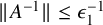 and
and

Then

Proof. The proof is based on the Neumann series argument similar to [Reference ShiShi22, Reference Liu and WangLW24]. For completeness, we give a proof.
First, we note that
$|A^{-1}(\boldsymbol {x},\boldsymbol {x}^{\prime })|\le \epsilon _1^{-1}e^{cM}e^{-c|\boldsymbol {x}-\boldsymbol {x}^{\prime }|}$
 for all
$\boldsymbol {x},\boldsymbol {x}^{\prime }\in X$
for all
$\boldsymbol {x},\boldsymbol {x}^{\prime }\in X$
 . For
$\boldsymbol {x}^0=\boldsymbol {x}, \boldsymbol {x}^s=\boldsymbol {x}'\in X$
. For
$\boldsymbol {x}^0=\boldsymbol {x}, \boldsymbol {x}^s=\boldsymbol {x}'\in X$
 and
$s\ge 1$
and
$s\ge 1$
 , we can obtain by direct computations that

Thus for
$s\ge 1$
 , one has

and for
$\boldsymbol {x}\neq \boldsymbol {x}',$


Hence, from the Schur’s test, we have

Using the Neumann series argument, we get

Thus

and for
$\forall \ \boldsymbol {x},\boldsymbol {x}'\in X$
 ,
,

We complete the proof.
In the following, let A be a matrix on
$\mathbb Z^{b+d}$
 satisfying

We introduce two types of coupling lemmas by iterating resolvent identities, which are repeatedly used to derive off-diagonal exponential decay estimates for Green’s functions.
Remark B.2. In (linear) spectral problems (cf. [Reference BourgainBou07, Reference Jitomirskaya, Liu and ShiJLS20]), one typically deals with operators such as

without the polynomial factor
$(|\boldsymbol {x}-\boldsymbol {x}'|+1)^{C_2}$
 . However, the extra polynomial factor does not significantly affect the proofs in [Reference Jitomirskaya, Liu and ShiJLS20] (cf. Lemma 3.2 and Theorem 3.3) and [Reference LiuLiu22] (cf. Theorem 2.1), as one can replace, at each step, the estimate

with

We say that an elementary region
$\Lambda \in \mathcal {ER}(L)$
 is in the class
$\mathbb G$
is in the class
$\mathbb G$
 (good) if (
$G_\Lambda =(R_{\Lambda }AR_{\Lambda })^{-1}$
(good) if (
$G_\Lambda =(R_{\Lambda }AR_{\Lambda })^{-1}$
 )
)

where
$\frac {1}{2}b_1< b_2\leq b_1$
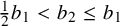 .
.
We have a revised version of the coupling lemma of [Reference LiuLiu22] (cf. also [Reference Bourgain, Goldstein and SchlagBGS02]).
Lemma B.3 (cf. Theorem 2.1, [Reference LiuLiu22])
Let
$\tilde {\Lambda }_0\in \mathcal {ER}(N)$
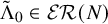 be an elementary region with the property that for all
$\Lambda \subset \tilde {\Lambda }_0,\Lambda \in \mathcal R_{L}^{\sqrt {N}}$
be an elementary region with the property that for all
$\Lambda \subset \tilde {\Lambda }_0,\Lambda \in \mathcal R_{L}^{\sqrt {N}}$
 with
$\sqrt N \leq L\leq N$
with
$\sqrt N \leq L\leq N$
 , the Green’s function
$(R_{\Lambda }A R_{\Lambda })^{-1}$
, the Green’s function
$(R_{\Lambda }A R_{\Lambda })^{-1}$
 satisfies

Assume that for any family
$\mathcal F$
 of pairwise disjoint elementary regions of size
$M=[ N^{\xi }]$
of pairwise disjoint elementary regions of size
$M=[ N^{\xi }]$
 contained in
$\tilde {\Lambda }_0,$
contained in
$\tilde {\Lambda }_0,$


Then for large N (depending on
$C_2, b_1$
 ), we have

where
$\vartheta =\vartheta \in (0,1)$
 is an absolute constant.
Remark B.4. There is an important difference between the original form of Lemma B.3 in [Reference LiuLiu22] and the present one. In [Reference LiuLiu22], (B.1)–(B.2) hold under the condition of
$|\boldsymbol {x}-\boldsymbol {x}'|\geq \frac {N}{10}$
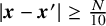 ,
$0<b_2\leq \frac {4}{5}b_1$
,
$0<b_2\leq \frac {4}{5}b_1$
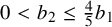 . However, the relation
$0<b_2\leq \frac {4}{5}b_1$
. However, the relation
$0<b_2\leq \frac {4}{5}b_1$
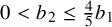 leads to the deterioration of decay rates in the Newton iteration when solving the P-equations. To address this issue, we impose a stronger restriction
$|\boldsymbol {x}-\boldsymbol {x}'|>N^{\frac 89}$
leads to the deterioration of decay rates in the Newton iteration when solving the P-equations. To address this issue, we impose a stronger restriction
$|\boldsymbol {x}-\boldsymbol {x}'|>N^{\frac 89}$
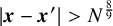 (this idea was first introduced in [Reference He, Shi, Shi and YuanHSSY20]), which ensures that
$0<b_2\leq b_1$
(this idea was first introduced in [Reference He, Shi, Shi and YuanHSSY20]), which ensures that
$0<b_2\leq b_1$
 . So Lemma B.3 is proved via the argument of [Reference LiuLiu22] combined with the argument of [Reference He, Shi, Shi and YuanHSSY20] (we can take
$b=\frac 34, \tau =\frac 12, \theta =\frac 89$
. So Lemma B.3 is proved via the argument of [Reference LiuLiu22] combined with the argument of [Reference He, Shi, Shi and YuanHSSY20] (we can take
$b=\frac 34, \tau =\frac 12, \theta =\frac 89$
 in Lemma 4.2 of [Reference He, Shi, Shi and YuanHSSY20]). We omit the details here.
We also need the following lemmas of [Reference Jitomirskaya, Liu and ShiJLS20] (with again minor modifications).
Lemma B.5 (cf. Lemma 3.2, [Reference Jitomirskaya, Liu and ShiJLS20])
Let
$M_0\geq (\log N)^{\frac {4}{3}},\ \frac {b_1}{2}<b_2\leq b_1$
 and
$M_1\leq N$
and
$M_1\leq N$
 . Suppose that
$\Lambda \subset \mathbb Z^{b+d}$
. Suppose that
$\Lambda \subset \mathbb Z^{b+d}$
 is connected and
$\mathrm {diam}(\Lambda )\leq 2N+1$
is connected and
$\mathrm {diam}(\Lambda )\leq 2N+1$
 . Suppose that for any
$\boldsymbol {y}\in \Lambda ,$
. Suppose that for any
$\boldsymbol {y}\in \Lambda ,$
 there exists some
$W=W(\boldsymbol {y})\in \mathcal E_M$
there exists some
$W=W(\boldsymbol {y})\in \mathcal E_M$
 with
$M_0\leq M\leq M_1$
with
$M_0\leq M\leq M_1$
 such that
$\boldsymbol {y}\in W\subset \Lambda ,\mathrm {dist}(\boldsymbol {y},\Lambda \setminus W)\geq \frac {M}{2}$
such that
$\boldsymbol {y}\in W\subset \Lambda ,\mathrm {dist}(\boldsymbol {y},\Lambda \setminus W)\geq \frac {M}{2}$
 and
and


Assume further that N is large enough such that

Then we have

Lemma B.6 (cf. Theorem 3.3, [Reference Jitomirskaya, Liu and ShiJLS20])
Assume
$\Lambda \subset \mathbb Z^{b+d}$
 is connected and
$\mathrm {diam}\ \Lambda \leq 2N+1$
is connected and
$\mathrm {diam}\ \Lambda \leq 2N+1$
 . Assume
$\mathrm {diam}\ \Lambda _1\leq N^{\frac {1}{2(b+d)}}$
. Assume
$\mathrm {diam}\ \Lambda _1\leq N^{\frac {1}{2(b+d)}}$
 . Let
$M_0\geq (\log N)^{\frac {4}{3}},\ \frac {b_1}{2}<b_2\leq b_1$
. Let
$M_0\geq (\log N)^{\frac {4}{3}},\ \frac {b_1}{2}<b_2\leq b_1$
 . Suppose that for any
$\boldsymbol {y}\in \Lambda ,$
. Suppose that for any
$\boldsymbol {y}\in \Lambda ,$
 there exists some
$W=W(\boldsymbol {y})\in \mathcal {ER}(M)$
there exists some
$W=W(\boldsymbol {y})\in \mathcal {ER}(M)$
 with
$M_0\leq M\leq N^{\frac 34}$
with
$M_0\leq M\leq N^{\frac 34}$
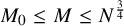 such that
$\boldsymbol {y} \in W\subset \Lambda , \mathrm {dist}(\boldsymbol {y},\Lambda \setminus \Lambda _1\setminus W)\geq \frac M2$
such that
$\boldsymbol {y} \in W\subset \Lambda , \mathrm {dist}(\boldsymbol {y},\Lambda \setminus \Lambda _1\setminus W)\geq \frac M2$
 and
and

Suppose that

Then

Remark B.7. A similar issue in Lemma B.3 also appears in Lemma B.5 and Lemma B.6. Again, we can improve the original estimates of [Reference Jitomirskaya, Liu and ShiJLS20] from
$|\boldsymbol {x}-\boldsymbol {x}'|\geq \frac {N}{10}$
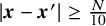 to
$|\boldsymbol {x}-\boldsymbol {x}'|\geq N^{\frac 89}.$
to
$|\boldsymbol {x}-\boldsymbol {x}'|\geq N^{\frac 89}.$
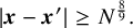
The following lemma deals with the projection property of elementary regions.
Lemma B.8. Let
$\Lambda \in \mathcal {ER}_{\mathbb Z^{b+d}}(N)$
 and denote by
$\Pi _b: \ \mathbb Z^{b+d} \to \mathbb Z^b$
and denote by
$\Pi _b: \ \mathbb Z^{b+d} \to \mathbb Z^b$
 the canonical projection map. Then for any
$\boldsymbol {k} \in \Pi _b\Lambda $
the canonical projection map. Then for any
$\boldsymbol {k} \in \Pi _b\Lambda $
 , the section

either belongs to
$\mathcal {ER}_{\mathbb Z^d}(N)$
 or is a rectangle of width at least N.
Proof. By translation invariance, it suffices to consider the regions centered at the origin, that is,
$\Lambda \in \mathcal {ER}_{\boldsymbol {0},\mathbb Z^{b+d}}(N)$
 . We proceed by analyzing the two possible forms of
$\Lambda $
. We proceed by analyzing the two possible forms of
$\Lambda $
 .
.
Case 1:
$\Lambda = \Lambda _{N,\mathbb Z^{b+d}} := [-N, N]^{b+d} \cap \mathbb Z^{b+d}$
 .
.
In this case, the section at any
$\boldsymbol {k} \in \Pi _b\Lambda $
 is simply
$\Lambda (\boldsymbol {k}) = [-N, N]^d \cap \mathbb Z^d$
is simply
$\Lambda (\boldsymbol {k}) = [-N, N]^d \cap \mathbb Z^d$
 , which belongs to
$\mathcal {ER}_{\mathbb Z^d}(N)$
, which belongs to
$\mathcal {ER}_{\mathbb Z^d}(N)$
 .
.
Case 2:
$\Lambda = \Lambda _{N,\mathbb Z^{b+d}}^{\boldsymbol {\iota }}$
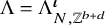 for some constraint vector
$\boldsymbol {\iota } = (\iota _i)_{1 \le i \le b+d} \in \{>, <, \emptyset \}^{b+d}$
for some constraint vector
$\boldsymbol {\iota } = (\iota _i)_{1 \le i \le b+d} \in \{>, <, \emptyset \}^{b+d}$
 with at least two nonempty components.
By definition,
$\Lambda $
 can be expressed as:

Using De Morgan’s laws, we can rewrite (B.3) as:

where the complement sets are given by

with the convention
$\overline {>} := <$
 and
$\overline {<} :=>$
and
$\overline {<} :=>$
 .
.
Note that the sectioning operation
$A \mapsto A(\boldsymbol {k}) = \{\boldsymbol {n}:\ (\boldsymbol {k},\boldsymbol {n}) \in A\}$
 has the following properties. Given
$A,B \in \mathbb {Z}^{b+d}$
has the following properties. Given
$A,B \in \mathbb {Z}^{b+d}$
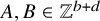 :
:
-
○ For $\boldsymbol {k} \in \prod _b (A \cup B)$
, one has
$(A \cup B)(\boldsymbol {k}) = A(\boldsymbol {k}) \cup B(\boldsymbol {k})$
since $$ \begin{align*} \{ \boldsymbol{n} : \ (\boldsymbol{k},\boldsymbol{n}) \in (A \cup B) \} = \{ \boldsymbol{n} : \ (\boldsymbol{k},\boldsymbol{n}) \in A \} \cup \{\boldsymbol{n} : \ (\boldsymbol{k},\boldsymbol{n}) \in B \}. \end{align*} $$
-
○ For $\boldsymbol {k} \in \prod _b (A \cap B)$
, one has
$(A \cap B)(\boldsymbol {k}) = A(\boldsymbol {k}) \cap B(\boldsymbol {k})$
since $$ \begin{align*} \{ \boldsymbol{n} : \ (\boldsymbol{k},\boldsymbol{n}) \in (A \cap B) \} = \{ \boldsymbol{n} : \ (\boldsymbol{k},\boldsymbol{n}) \in A \} \cap \{\boldsymbol{n} :\ (\boldsymbol{k},\boldsymbol{n}) \in B \}. \end{align*} $$






Therefore, for a fixed
$\boldsymbol {k} \in \Pi _b\Lambda $
 , taking the section of (B.4) yields:

We now analyze the sections of the complements for
$1 \le i \le b+d$
 . If
$\iota _i = \emptyset $
. If
$\iota _i = \emptyset $
 , the section is trivially empty. Thus it is sufficient to consider the case
$\iota _i \neq \emptyset $
, the section is trivially empty. Thus it is sufficient to consider the case
$\iota _i \neq \emptyset $
 . We decouple the Cartesian product
$\boldsymbol {x} \in \mathbb Z^{b+d}$
. We decouple the Cartesian product
$\boldsymbol {x} \in \mathbb Z^{b+d}$
 as
$(\boldsymbol {k},\boldsymbol {n}) \in \mathbb Z^b \times \mathbb Z^d$
as
$(\boldsymbol {k},\boldsymbol {n}) \in \mathbb Z^b \times \mathbb Z^d$
 :
:

Combining (B.5) and (B.6), we observe that if there exists any
$1 \le i \le b$
 such that
$k_i \ \overline {\iota _i} \ 0$
such that
$k_i \ \overline {\iota _i} \ 0$
 (
$\iota _i \neq \emptyset $
(
$\iota _i \neq \emptyset $
 ), the union in (B.5) evaluates to
$\mathbb Z^d$
), the union in (B.5) evaluates to
$\mathbb Z^d$
 . In this scenario,
$\Lambda (\boldsymbol {k}) = \Lambda _{N,\mathbb Z^d}$
. In this scenario,
$\Lambda (\boldsymbol {k}) = \Lambda _{N,\mathbb Z^d}$
 , which belongs to
$\mathcal {ER}_{\mathbb Z^d}(N)$
, which belongs to
$\mathcal {ER}_{\mathbb Z^d}(N)$
 .
.
Otherwise, the first b constraints do not contribute to the union, and the geometric shape is entirely determined by the remaining d spatial constraints. Thus, there exists a projected constraint vector
$\boldsymbol {\iota }' \in \{>, <, \emptyset \}^{d}$
 such that

Substituting this back into (B.5) and applying De Morgan’s laws once more, we obtain

Let
$|\boldsymbol {\iota }'|$
 denote the number of nonempty components (i.e.,
$\iota _j' \neq \emptyset $
denote the number of nonempty components (i.e.,
$\iota _j' \neq \emptyset $
 ) in
$\boldsymbol {\iota }'$
) in
$\boldsymbol {\iota }'$
 . We classify
$\Lambda (\boldsymbol {k})$
. We classify
$\Lambda (\boldsymbol {k})$
 as follows:
-
○ If $ |\boldsymbol {\iota }'| = 0 $
, then
$\Lambda (\boldsymbol {k}) = \Lambda _{N,\mathbb Z^d}$
, which belongs to
$\mathcal {ER}_{\mathbb Z^d}(N)$
. -
○ If $ |\boldsymbol {\iota }'| = 1 $
,
$\Lambda (\boldsymbol {k})$
is the full box
$\Lambda _{N,\mathbb Z^d}$
minus a single half-space. This leaves a rectangle where
$(d-1)$
sides have length
$2N$
and one side has length N. Hence, it is a rectangle of width at least N. -
○ If $ |\boldsymbol {\iota }'| \ge 2 $
, by the definition,
$\Lambda (\boldsymbol {k}) = \Lambda _{N,\mathbb Z^d}^{\boldsymbol {\iota }'}$
, which implies
$\Lambda (\boldsymbol {k}) \in \mathcal {ER}_{\mathbb Z^d}(N)$
.




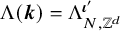

This completes the proof for the origin-centered case.
Acknowledgments
The authors would like to thank the handling editor and the anonymous reviewers for valuable suggestions.
Competing interests
The authors have no competing interests to declare.
Financial support
Y. Shi was supported by the National Key R&D Program (2021YFA1001600) and the NSFC (12522110). W.-M. Wang acknowledges support from the CY Initiative of Excellence, “Investissements d’Avenir” Grant No. ANR-16-IDEX-0008.


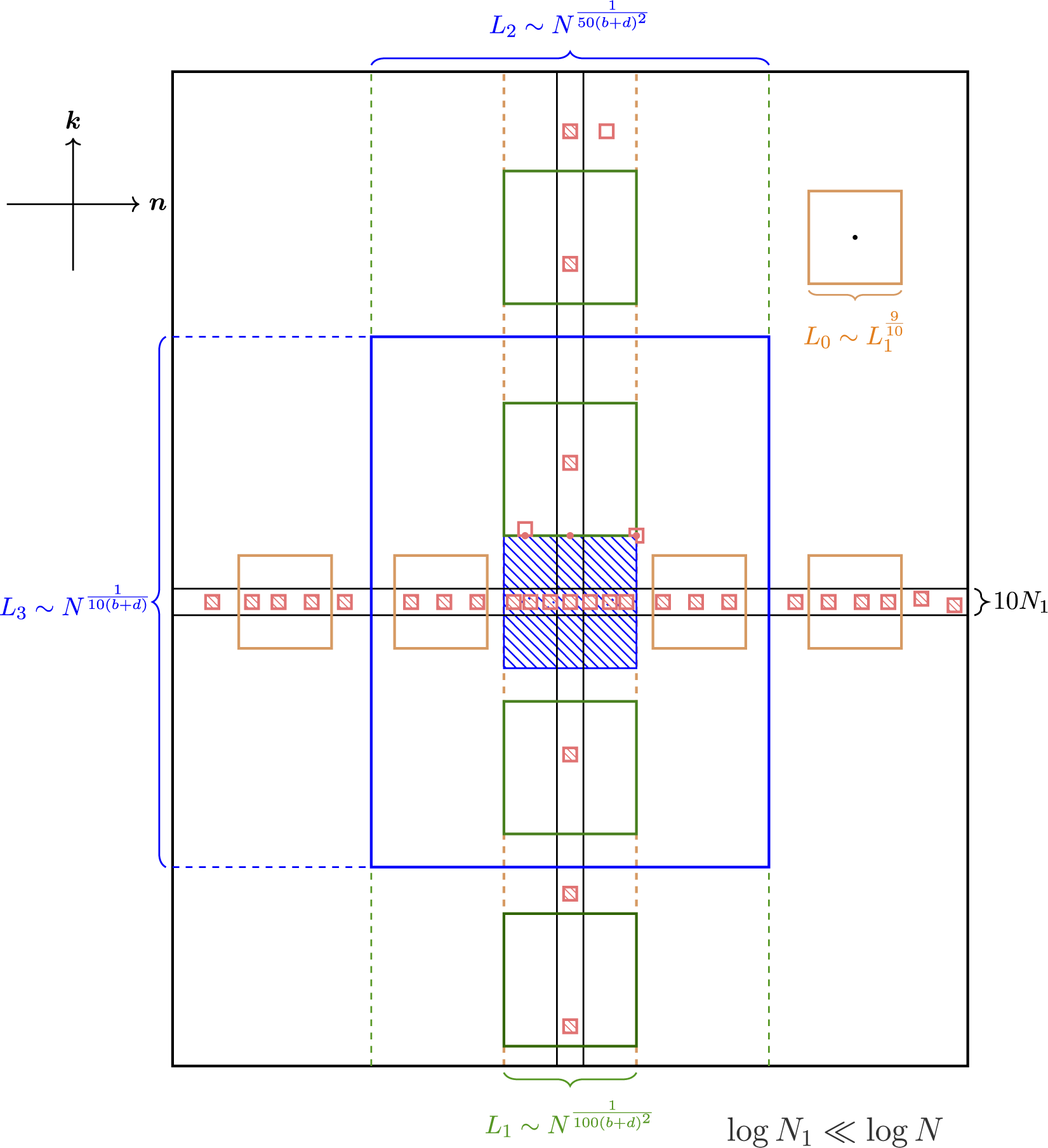

 Open access

