2.1. Zero-dimensional ignition dataset for a homogeneous hydrogen/air mixture

In a spatially homogeneous constant volume reactor, the temporal evolution of species and temperature starting from the initial time, $ t $ = 0, is computed by solving the system of ordinary differential equations (ODEs) defined by

(2.1) $$ \frac{d\boldsymbol{\theta}}{dt}={\dot{\boldsymbol{\omega}}}_{\boldsymbol{\theta}},t\in \left[0,{t}_f\right] $$

where $ \boldsymbol{\theta} $ represents the thermochemical state vector (i.e., species mass fraction and temperature), $ {\dot{\boldsymbol{\omega}}}_{\boldsymbol{\theta}} $ the reaction rate vector divided by the mixture density, and $ {t}_f $ the end time. For the initial conditions, the initial pressure of the system, $ {p}_0 $ , is fixed to be atmospheric, and different values for the initial temperature, $ {T}_0 $ , are used including 1000, 1050, 1100, 1300, and 1400 K. The initial mass fractions of the hydrogen/air mixture are determined by an equivalence ratio, $ \phi $ , which ranges from 0.1 to 3.0. A detailed chemical kinetic mechanism for hydrogen/air mixtures, developed by Li et al. (Reference Li, Zhao, Kazakov and Dryer2004), is used where the dimension of the original thermochemical state vector is 10. A six-stage, fourth-order Runge–Kutta method (Kennedy and Carpenter, Reference Kennedy and Carpenter1994) with a uniform time step, dt, of 0.2 ns is adopted for time integration. The CHEMKIN library (Kee et al., Reference Kee, Rupley, Meeks and Miller1996) is used to compute the chemical kinetics and thermodynamic properties of the mixture.

Figure 1 shows the ignition delay time, $ {\tau}_{\mathrm{ig}} $ , of the hydrogen/air mixture for various $ \phi $ and $ {T}_0 $ . As expected, the variation in $ {\tau}_{\mathrm{ig}} $ exhibits a “U”-shaped profile as a function of $ \phi $ . Here, $ {\tau}_{\mathrm{ig}} $ is defined as the time at which the temperature gradient is maximum. In accordance with Arrhenius Law, $ {\tau}_{\mathrm{ig}} $ notably changes with changes in $ {T}_0 $ .

Figure 1.

Variations in 0D ignition delay time, $ {\tau}_{\mathrm{ig}} $ , of the hydrogen/air mixture for different initial temperatures, $ {T}_0 $ , as a function of equivalence ratio, $ \phi $ . In the present study, it is assumed that the number of training samples at the source task ( $ {T}_0 $ = 1000 K) is sufficient, while the number of training samples at the target tasks ( $ {T}_0> $ 1000 K) is sparse.

In the present study, the objective of the PC-transport ROM is to replicate the ignition characteristics of the hydrogen/air mixture over a wide range of $ \phi $ at a specific $ {T}_0 $ , meaning that training samples, the low-dimensional manifold, and the corresponding ANN model are separated by $ {T}_0 $ . To reasonably provide a data-sparse scenario, an underlying assumption of the present study is that there exists a sufficient number of training samples spanning over $ \phi $ at $ {T}_0 $ of 1000 K, while the training data size for the cases where $ {T}_0> $ 1000 K is assumed to be sparse (see the symbols in Fig. 1 as an example).

Specifically, at $ {T}_0= $ 1000 K, the training dataset is collected by carrying out 30 different 0D simulations varying $ \phi $ (i.e., $ \Delta \phi $ = 0.1; $ \phi $ ranging from 0.1 to 3.0), and then the low-dimensional manifold is defined by applying PCA to the training dataset. Training of the ANN model by using a sufficient number of training samples at $ {T}_0= $ 1000 K is considered as the “source task” for the present study. Here, $ {N}_{\phi } $ is defined as the number of 0D simulations at a given $ {T}_0 $ such that $ {N}_{\phi } $ of the source task is 30. For the “target tasks” where $ {T}_0 $ is higher than 1000 K (i.e., 1050, 1100 1300, and 1400 K), $ {N}_{\phi } $ is set to be ≤4, such that the number of training data for the target task is forced to be sparse. In this study, a “sparse dataset” refers to a dataset with insufficient training samples such that the corresponding ANN model is unable to replicate the ignition characteristics of a fuel/air mixture with a wide range of $ \phi $ (i.e., $ \phi =0.1-3.0 $ ) at a given $ {T}_0 $ . The description of the dataset with different $ {N}_{\phi } $ is summarized in Table 1. Note that the range of $ {T}_0 $ (i.e., 1000 $ \le {T}_0\le 1400 $ K) is carefully selected to ensure that the overall distributions of the input and output datasets between the source and target tasks are similar, yet noticeably different. This difference becomes more pronounced as $ {T}_0 $ increases in the target task.

Table 1.

Description of the dataset with different $ {N}_{\phi } $

While the present study provides a data-sparse scenario based on a series of 0D simulations, such an imbalance in the number of training samples can also be observed from multidimensional simulations and experiments (Humbird et al., Reference Humbird, Peterson, Spears and McClarren2020; Subel et al., Reference Subel, Chattopadhyay, Guan and Hassanzadeh2021). It is also noted that transfer learning methods used in the present study are not limited to specific source and target tasks. Rather, these methods can be applied to various scenarios (e.g., different pressure or equivalence ratio conditions between source and target tasks), provided that there is a task similarity between the two tasks.

For each 0D simulation, the thermochemical state vector and their reaction rate, $ \theta $ and $ {\dot{\omega}}_{\theta } $ , respectively, are uniformly sampled from $ t $ of 0 to 2 $ {\tau}_{\mathrm{ig}} $ . The number of samples for each 0D simulation is set to be 20,000 such that the first 10,000 samples are assigned to the preignition period and the remaining 10,000 samples are related to the postignition period. The “test dataset” at a given $ {T}_0 $ is also prepared to evaluate the accuracy of the PC-transport ROM. It consists of 29 different 0D simulation results at a given $ {T}_0 $ ( $ \Delta \phi $ = 0.1; $ \phi $ ranging from 0.15 to 2.95) and is separated from the training dataset.

2.2. Principal component analysis

Consistent with previous studies applying PC-transport ROMs (Parente et al., Reference Parente, Sutherland, Tognotti and Smith2009; Sutherland and Parente, Reference Sutherland and Parente2009; Mirgolbabaei and Echekki, Reference Mirgolbabaei and Echekki2013, Reference Mirgolbabaei and Echekki2014), the dimension of the original thermochemical vector is reduced by applying PCA. Assuming that $ M $ number of samples of the N-dimensional thermochemical state vectors are collected by performing multiple 0D simulations at a given $ {T}_0 $ , the dataset of the thermochemical vector, $ \boldsymbol{\Theta} $ = [ $ {\boldsymbol{\theta}}_1 $ , $ {\boldsymbol{\theta}}_2 $ , …, $ {\boldsymbol{\theta}}_M $ ], is composed of a $ N\times M $ dimensional matrix. Note that $ \boldsymbol{\Theta} $ is normalized based on the min–max normalization before PCA. The $ N\times N $ dimensional matrix of orthonormal eigenvectors, Q $ {}^T $ , of the covariance matrix of $ \boldsymbol{\Theta} $ is constructed, and subsequently, the dataset of the PC vector, $ \boldsymbol{\Psi} $ , can be defined as

(2.2) $$ \boldsymbol{\Psi} ={\mathbf{Q}}^{\mathrm{T}}\boldsymbol{\Theta} $$

where $ \boldsymbol{\Psi} \in {\mathrm{\mathbb{R}}}^{N\times M} $ represents the $ M $ numbers of collections of the PC vector, $ \boldsymbol{\psi} = $ [ $ {\psi}_1 $ , $ {\psi}_2 $ , …, $ {\psi}_N $ ] $ {}^{\mathrm{T}} $ .

Note that the first PC, $ {\psi}_1 $ , is a linear combination of the original thermochemical state vector that captures the maximum variance of the dataset. The second PC, $ {\psi}_2 $ , is then orthogonal to the first PC, and all the subsequent PCs follow the same concept. In the present study, the leading first five PCs (i.e., $ {N}_{\mathrm{PC}} $ = 5) are retained from $ \boldsymbol{\psi} $ such that the dimensionality of the system is reduced from 9 (except for N $ {}_2 $ ) to 5, which captures over 99% of the original total variance. In other words, a $ N\times {N}_{\mathrm{PC}} $ matrix of $ \mathbf{A} $ is constructed that contains the leading $ {N}_{\mathrm{PC}} $ eigenvectors from $ \mathbf{Q} $ . The low-dimensional manifold then becomes

(2.3) $$ {\boldsymbol{\Psi}}^{red}={\mathbf{A}}^{\mathrm{T}}\boldsymbol{\Theta} $$

where $ {\boldsymbol{\Psi}}^{red}\in {\mathrm{\mathbb{R}}}^{N_{\mathrm{PC}}\times M} $ represents the dataset of the truncated PC vector, $ \left({\boldsymbol{\psi}}^{red}\right) $ = [ $ {\psi}_1 $ , $ {\psi}_2 $ , …, $ {\psi}_{N_{\mathrm{PC}}} $ ] $ {}^{\mathrm{T}} $ . Hereinafter, $ {\boldsymbol{\Psi}}^{red} $ and $ {\boldsymbol{\psi}}^{red} $ are referred to as $ \boldsymbol{\Psi} $ and $ \boldsymbol{\psi} $ , respectively, for the sake of brevity.

The system of ODEs for the low-dimensional manifold can be defined by projecting Eq. 2.1 on the matrix $ {\mathbf{A}}^{\mathrm{T}} $ :

(2.4) $$ \frac{d\boldsymbol{\psi}}{dt}={\dot{\omega}}_{\boldsymbol{\psi}},t\in \left[0,{t}_f\right] $$

where $ {\dot{\omega}}_{\boldsymbol{\psi}} $ is the reaction rate term for $ \boldsymbol{\psi} $ , defined by $ {\dot{\boldsymbol{\omega}}}_{\boldsymbol{\psi}} $ = $ {\mathbf{A}}^{\mathrm{T}}{\dot{\boldsymbol{\omega}}}_{\boldsymbol{\theta}} $ (Sutherland and Parente, Reference Sutherland and Parente2009). In the framework of the PC-transport ROM, the time integration of Eq. 2.4 is solved instead of solving Eq. 2.1, and then a conversion from $ \boldsymbol{\psi} $ into $ \boldsymbol{\theta} $ is carried out as a postprocessing step. An ANN model is used for the regression of $ {\dot{\boldsymbol{\omega}}}_{\boldsymbol{\psi}} $ as a function of $ \boldsymbol{\psi} $ .

Figure 2 shows the PC modes with respect to the original thermochemical vector defined by using different training datasets in terms of $ {T}_0 $ . For all the cases, $ {N}_{\phi } $ is set to be 30. It is readily observed from the figure that the PC modes show a similar trend irrespective of the dataset, implying that transfer learning can be effectively applied to the dataset. This result is consistent with the previous study (Biglari and Sutherland, Reference Biglari and Sutherland2012) which shows that the PCA basis is insensitive to the spatial filter width in the context of large eddy simulations. Specifically, the first PC mode is negatively correlated with the fuel and oxidizer, while it is positively correlated with the product, H₂O, and temperature. Accordingly, the first PC represents the oxidation progress of the hydrogen/air mixture. The second PC mode is primarily correlated with the fuel, and the third PC mode is correlated with the formation of HO₂. The results indicate that the PCs obtained through the data-driven approach are linked to a physical interpretation of the combustion system, consistent with previous findings (Owoyele and Echekki, Reference Owoyele and Echekki2017; Malik et al., Reference Malik, Vega, Coussement and Parente2021).

Figure 2.

Modes of the first five PCs depending on the training dataset varying $ {T}_0 $ with $ {N}_{\phi } $ of 30.

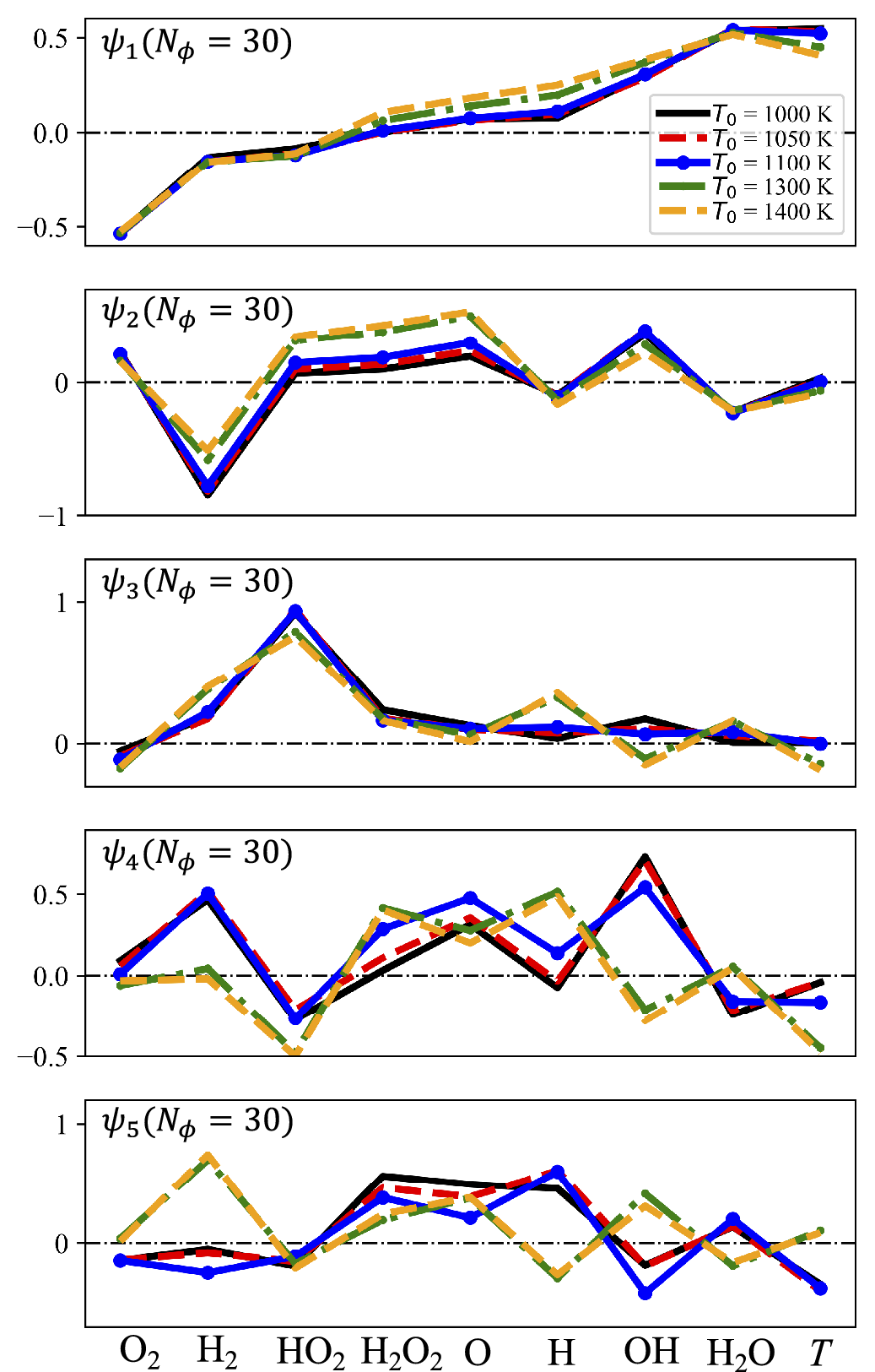
Nonetheless, it is important to note that the PC modes are slightly altered with a change of $ {T}_0 $ , which can have a significant impact on the application of transfer learning to the ROM. In other words, a unified definition of the low-dimensional manifold throughout tasks would be preferred to transfer the knowledge efficiently. In the present study, $ {\mathbf{A}}^{\mathrm{T}} $ defined from the source task (i.e., $ {N}_{\phi }=30 $ and $ {T}_0 $ = 1000 K) is applied to all target tasks to ensure consistency in the definitions of $ \boldsymbol{\psi} $ and $ {\dot{\boldsymbol{\omega}}}_{\boldsymbol{\psi}} $ . Such an approach is based on the observation that despite the presence of slight differences in the PC modes, the first PC, which also accounts for most of the data variance, also exhibits the least difference when $ {T}_0 $ is varied.

Note, however, that using a unified $ {\mathbf{A}}^{\mathrm{T}} $ has a potential risk of introducing noticeable errors during the conversion from $ \boldsymbol{\psi} $ to $ \boldsymbol{\theta} $ in the target task, especially if the reconstruction is carried out by using a matrix conversion step, $ \boldsymbol{\theta} \approx \mathbf{A}\;\boldsymbol{\psi} $ . To address this issue, another non-linear ANN model is employed to convert from $ \boldsymbol{\psi} $ to $ \boldsymbol{\theta} $ for all cases, instead of using the matrix inversion. This ensures that the performance of the reconstruction is mainly affected by the number of samples, $ M $ , in the target task rather than the choice of $ {\mathbf{A}}^{\mathrm{T}} $ . As will be discussed, such an ANN model is found to require far fewer parameters compared with the other ANN models that predict $ {\dot{\boldsymbol{\omega}}}_{\boldsymbol{\psi}} $ . Hence, this ANN model shows a reasonable accuracy even when trained with a sparse dataset. It is also noted that the non-linear ANN was found to reduce the reconstruction error during the conversion from $ \boldsymbol{\psi} $ to $ \boldsymbol{\theta} $ as compared with the matrix inversion, $ \boldsymbol{\theta} \approx \mathbf{A}\;\boldsymbol{\psi} $ (Mirgolbabaei and Echekki, Reference Mirgolbabaei and Echekki2015).

The sensitivity of the ANN model performance depending on the definition of the eigenvector matrix, $ {\mathbf{A}}^{\mathrm{T}} $ , is shown in Fig. S1 in Supplementary Material (SM). It is shown that the effect of a PCA basis (i.e., $ {\mathbf{A}}^{\mathrm{T}} $ ) plays a secondary role in determining the optimal ANN model in the target task, while the main source of the error arises from the source term regression errors.

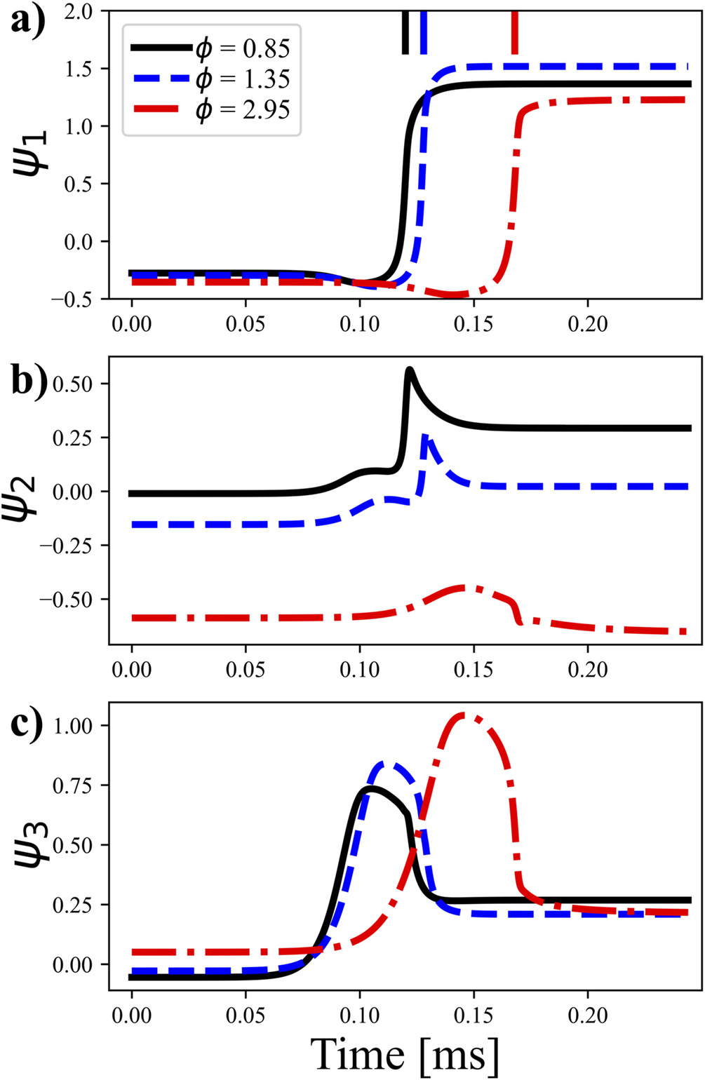
Figure 3 shows the temporal evolution of the first three PCs for three different $ \phi $ of 0.85, 1.35, and 2.95 at $ {T}_0 $ of 1000 K, obtained by projecting the FOM result onto $ {\mathbf{A}}^{\mathrm{T}} $ . As discussed earlier, the first PC represents the progress variable of the mixture, such that the first PC switches from negative to positive values near the ignition delay time. For the third PC, its mode is mainly correlated with the intermediate species, namely HO₂, such that it is maximum just before ignition of the mixture.

Figure 3.

Temporal evolution of the first three PCs for three different equivalence ratios, $ \phi $ , of 0.85, 1.35, and 2.95, obtained by projecting $ {\mathbf{A}}^{\mathrm{T}} $ onto the FOM result. The vertical lines in (a) represent the ignition delay time for different $ \phi $ . Here, the ignition delay time is defined by the time at which the temperature gradient reaches its maximum value.

2.3. Artificial neural network

A fully connected, multi-input, and multi-output ANN model is used to predict the reaction rates of the PCs. The PC vector is used as the input of the ANN, and the reaction rates of these PCs are the output. The architecture of the ANN model is determined by performing a grid search method from which the number of hidden layers and nodes are set to 3 and 30, respectively. The hyperbolic tangent activation function is adopted for all hidden layers. For cases without the application of transfer learning methods, the Xavier normal initialization method (Glorot and Bengio, Reference Glorot and Bengio2010), which is a commonly used initialization scheme and is compatible with the hyperbolic tangent activation function, is employed. Note that the goal of training the ANN model is to optimize weights ( w ) and biases ( b ) vectors, which together make up the parameter vector, h  = [ w , b ]. We apply the early stopping callback function based on the validation loss, and a plateau learning rate scheduler is used to fine-tune the parameters.

As discussed in Section 2.2, another ANN model is also employed and trained for the reconstruction from $ \boldsymbol{\psi} $ to $ \boldsymbol{\theta} $ . One hidden layer with 10 nodes is found to be sufficient for this ANN model to reconstruct the original thermochemical scalars with reasonable accuracy. Note that such an ANN model requires considerably fewer training samples, and, therefore, transfer learning is not applied to this model.

For both source and target tasks, 80% of the dataset is used as a training dataset, and the remaining 20% is allocated as the validation set to assess the model’s performance and prevent overfitting. The mean absolute error (MAE) loss function is applied for the ANN training, consistent with previous studies showing that the choice of the MAE results in a better performance than RMSE and MSE in capturing an ignition process of a fuel/air mixture (Han et al., Reference Han, Jia, Chang and Li2020, Reference Han, Jia, Chang and Li2022). The Adam optimizer (Kingma and Ba, Reference Kingma and Ba2014) is used for stochastic optimization. Once the ANN model is optimized using the training dataset, it is both a priori and a posteriori evaluated against the test dataset, which is not involved in the training process.

To efficiently capture the ignition process of the hydrogen/air mixture, the dataset is divided into three clusters (Cl#1–Cl#3): (Cl#1) earlier ignition period ( $ {\psi}_3-{\psi}_{3,0}< $ 0.005 and $ {\psi}_1<0.0 $ ), (Cl#2) later ignition period ( $ {\psi}_3-{\psi}_{3,0}\ge $ 0.005 and $ {\psi}_1<0.0 $ ), and (Cl#3) post ignition period ( $ {\psi}_1\ge 0.0 $ ), where the $ {\psi}_{3,0} $ denotes the magnitude of $ {\psi}_3 $ at the initial condition. The clustering criteria are based on the observation that $ {\psi}_1 $ and $ {\psi}_3 $ effectively represent the progress variable and evolution of intermediate species, respectively, as depicted in Figure 3. For more complicated numerical configurations, unsupervised clustering algorithms (e.g., k-means algorithm or Vector Quantization Principal Component Analysis [VQPCA]) could be adopted to automatically determine the clustering criteria, as described in (D’Alessio et al., Reference D’Alessio, Sundaresan and Mueller2023; Savarese et al., Reference Savarese, Jung, Dave, Chen and Parente2024). Note that the data clustering method has been proven as an effective way to capture the ignition process of various fuel/air mixtures (Han et al., Reference Han, Jia, Chang and Li2020; Han et al., Reference Han, Jia, Chang and Li2022; Jung, Kumar, et al., Reference Jung, Kumar, Echekki and Chen2024). The performance of the ROM will later be evaluated in each cluster.

2.4. Transfer learning methods

In this study, four different transfer learning methods are applied to the target tasks. Let h $ {}^s $ denote the parameter vector (weights and biases vectors) extracted from the pretrained source task. The first transfer learning method (TL1) is that the knowledge of the pretrained ANN model obtained from the source task is fully shared with the target task. In other words, the parameter vector in the target task, denoted by h , is identical to h $ {}^s $ , and no fine-tuning step is performed in TL1. Therefore, it can be conjectured that TL1 is likely to show good performance only when the task similarity between the source and target is very high. The second transfer learning method (TL2) is to set the initial parameter vector in the target task, h $ {}_0 $ , with h $ {}^s $ , and then fine-tune the model using the sparse dataset in the target task. In other words, TL2 serves to initialize the ANN model in the target task by using h $ {}^s $ , and as such, h will be different from h $ {}^s $ after fine-tuning.

As discussed in Li et al. (Reference Li, Grandvalet and Davoine2029), a drawback of TL2 is that previous knowledge obtained from the source task may be lost during the fine-tuning step. To resolve this issue, the third transfer learning method (TL3), which is associated with parameter restriction, is applied. The total loss function, $ \mathrm{\mathcal{L}} $ , in TL3 includes a regularization term (X. Li et al., Reference Li, Grandvalet and Davoine2018, Reference Li, Grandvalet and Davoine2029), which is slightly different from the conventional $ {l}_2 $ regularizer, as follows:

(5) $$ \mathrm{\mathcal{L}}=\mathrm{MAE}+{\lambda}_1\parallel \boldsymbol{h}-{\boldsymbol{h}}^s{\parallel}_2^2. $$

In this expression, MAE represents the mean absolute error loss function, and $ {\lambda}_1 $ is the regularization parameter. Here, the magnitude of $ {\lambda}_1 $ mainly controls the degree of knowledge transferred from source to target task during the fine-tuning step in the target task. Consistent with TL2, h $ {}_0 $ in TL3 is set to be h $ {}^s $ , and subsequently, the ANN model is fine-tuned by using the dataset in the target task. It is evident that $ \boldsymbol{h} $ will be identical to h $ {}^s $ as the magnitude of $ {\lambda}_1 $ is very high, whereas there is no penalty for $ \boldsymbol{h} $ to change during the fine-tuning step at $ {\lambda}_1=0 $ . Therefore, it can be considered that TL3 becomes equivalent to TL1 and TL2 as the magnitude of $ {\lambda}_1 $ becomes very large or approaches zero, respectively.

Lastly, we introduce a novel transfer learning method called “Parameter control via Partial Initialization and Regularization (PaPIR).” The central idea of PaPIR is to provide a unified transfer learning framework in terms of initialization and regularization. In addition to applying $ {\lambda}_1 $ to adjust the effect of the regularization during training, another variable, $ {\lambda}_2 $ , is introduced in PaPIR so that the amount of previous knowledge transferred to the target task in terms of the initialization can also be controlled by changing the magnitude of $ {\lambda}_2 $ . The initialization method of the PaPIR is a combination of two initialization schemes, namely Xavier normal initialization (Glorot and Bengio, Reference Glorot and Bengio2010) and initialization with h $ {}^s $ . Xavier normal initialization is a family of the Gaussian-based initialization technique with zero mean and a determined variance. Thus, it is a sort of random initialization strategy and is unrelated to the pretrained knowledge. On the other hand, initialization with h $ {}^s $ is categorized as a data-driven initialization strategy (Narkhede et al., Reference Narkhede, Bartakke and Sutaone2022).

The initialization process in PaPIR follows a normal distribution function, $ N $ , which is expressed as follows:

(2.6) $$ {\boldsymbol{w}}_0=N\left({\lambda}_2{\boldsymbol{w}}^s,{\left[\sqrt{\frac{2}{f_i+{f}_o}}\left(1-{\lambda}_2\right)\right]}^2\right) $$

(2.7) $$ {\boldsymbol{b}}_{0,b}=N\left({\lambda}_2{\boldsymbol{b}}^s,{0}^2\right) $$

where $ N $ (m, $ {\sigma}^2 $ ) represents the mean (m) and standard deviation ( $ \sigma $ ) of the normal distribution function, w $ {}_0 $ and b $ {}_0 $ represent the initial weights and biases vector of the ANN model in the target task (i.e., h $ {}_0 $ = [ w $ {}_0 $ , b $ {}_0 $ ]), and w $ {}^s $ and b $ {}^s $ represent the weight and biases vector extracted from the source task (i.e., h $ {}^s $ = [ w $ {}^s $ , b $ {}^s $ ]). Here, $ {f}_{\mathrm{i}} $ and $ {f}_{\mathrm{o}} $ represent the number of incoming and outgoing nodes at each layer, respectively, which are identical to those used in the Xavier normal initialization scheme (Glorot and Bengio, Reference Glorot and Bengio2010).

As $ {\lambda}_2 $ in Eqs. 2.6–2.7 approaches zero, the initialization scheme becomes equivalent to the Xavier normal initialization method. As $ {\lambda}_2 $ approaches unity, on the other hand, h $ {}_0 $ simply becomes identical to h $ {}^s $ . Thus, the degree of knowledge transfer for the initialization of the target task can be adjusted by varying the value of $ {\lambda}_2 $ between zero and unity, which equivalently represents a bound between the Xavier normal initialization method and h $ {}^s $ , respectively. As demonstrated in Section 3, PC-transport ROM with a sparse dataset generally fails to capture the overall ignition process of a hydrogen/air mixture if the ANN model is trained from scratch. This shortcoming is mainly attributed to the propensity of the ANN models to get stuck in local minima, especially with a sparse dataset. Given that an appropriate initialization scheme can help avoid local minima (Narkhede et al., Reference Narkhede, Bartakke and Sutaone2022), PaPIR has the potential advantage of enhancing the performance of transfer learning by introducing some degree of randomness during the initialization process. Table 2 summarizes and compares the four transfer learning methods used in the present study.

Table 2.

Summary of the transfer learning methods used in this study. “ $ \alpha $ ” in the PaPIR model represents $ \alpha $ = $ \sqrt{\Big(2/\left({f}_i+{f}_o\right)}\left(1-{\lambda}_2\right) $

3.1. Source task: $ {T}_0= $ 1000 K

In the source task, the ANN models for predicting the reaction rate of PCs are trained by using the training dataset with $ {N}_{\phi } $ of 30 ( $ \phi =0.1-3.0 $ ; $ \Delta \phi $ = 0.1) at $ {T}_0 $ of 1000 K. A system of ODEs, Eq. 2.4, is solved for 29 different 0D simulations listed in the test dataset, and then the performance of the PC-transport ROM is evaluated against the FOM by comparing $ {\tau}_{\mathrm{ig}} $ between two different simulations. As mentioned earlier, $ {\tau}_{\mathrm{ig}} $ is defined by the time at which the temperature gradient reaches its maximum value, and $ {\tau}_{\mathrm{ig}} $ in the PC-transport ROM can be predicted after reconstructing the temperature profile from the evolved PC solutions.

Figure 4 shows the variations in $ {\tau}_{\mathrm{ig}} $ for the hydrogen/air mixture at $ {T}_0 $ = 1000 K with various $ \phi $ predicted by the PC-transport ROM and FOM. As shown in the figure, $ {\tau}_{\mathrm{ig}} $ predicted by the PC-transport ROM shows excellent agreement with the FOM. The relative percentage error is below 2% for the entire range of $ \phi $ , demonstrating that PC-transport ROM with a sufficient number of training samples can accurately reproduce the ignition process of a hydrogen/air mixture over a wide range of $ \phi $ at a given $ {T}_0 $ . Note that the relative percent error for the fuel-lean mixture is slightly higher than that for the fuel-rich mixture, which is attributed to the fact that the number of training samples assigned to the fuel-lean mixture is fewer than that assigned to the fuel-rich mixture. Also, $ {\tau}_{\mathrm{ig}} $ shows a steeper variation with $ \phi $ as $ \phi $ becomes less than 0.5, which also affects the result.

Figure 4.

Variations in (a) 0D ignition delay time, $ {\tau}_{\mathrm{ig}} $ , predicted by FOM (solid symbol) and PC-transport ROM (dashed-dot line), and (b) the relative error of the PC-transport ROM compared with FOM for the homogeneous hydrogen/air mixture with various $ \phi $ (i.e., $ \phi $ = 0.15–2.95; $ \Delta \phi $ =0.1) at $ {T}_0 $ = 1000 K.

Figure 5 presents the temporal evolution of the original thermochemical state vector of the hydrogen/air mixture at $ {T}_0 $ of 1000 K and $ \phi $ of 1.35, as predicted by the PC-transport ROM and FOM. It is readily observed that the profiles of the thermochemical state variables reconstructed from the PC-transport ROM are in good agreement with the results from FOM for both major and minor species. This finding indicates that the number of PCs retained in this study ( $ {N}_{\mathrm{PC}}= $ 5) is sufficient to recover the original thermochemical state scalars, together with the successful validation of using the ANN model to convert from $ \boldsymbol{\psi} $ to $ \boldsymbol{\theta} $ .

Figure 5.

Temporal evolution of the thermochemical state scalars of a homogeneous hydrogen/air mixture at $ {T}_0 $ = 1000 K and $ \phi $ = 1.35. Solid line: FOM result, Dashed line: reconstructed from the PC-transport ROM result with $ {N}_{\phi } $ = 30.

3.2. Target task with data sparsity

The results of the PC-transport ROM for a target task where $ {T}_0 $ is 1050 K are investigated depending on the number of training samples. In this task, ANN models are trained by using each of the different training datasets, each with different numbers of training samples (i.e., $ {N}_{\phi } $ = 2 $ - $ 30), and both a priori and a posteriori evaluations are carried out to assess the performance of the ROM depending on $ {N}_{\phi } $ . At a given $ {N}_{\phi } $ , the ANN model training is repeated 10 times to take into account the sensitivity of the model arising from the randomness of the initial parameters and the stochastic nature of the optimization process. The best achievable (or minimum) error is then evaluated over 10 repetitions at a given $ {N}_{\phi } $ . The normalized root mean squared error (NRMSE) is adopted to a priori quantify the error of the ANN for predicting $ {\dot{\boldsymbol{\omega}}}_{\boldsymbol{\psi}} $ and is defined by

(2.8) $$ \mathrm{NRMSE}\left[\%\right]=\sqrt{\frac{\parallel {\hat{\boldsymbol{\omega}}}_{\boldsymbol{\psi}, p}-{\hat{\boldsymbol{\omega}}}_{\boldsymbol{\psi}}{\parallel}_2^2}{\parallel {\hat{\boldsymbol{\omega}}}_{\boldsymbol{\psi}}{\parallel}_2^2}}\times 100 $$

where $ {\hat{\boldsymbol{\omega}}}_{\boldsymbol{\psi}, p} $ and $ {\hat{\boldsymbol{\omega}}}_{\boldsymbol{\psi}} $ represent the normalized reaction rates of the PC vector predicted by the ANN model and obtained from the FOM, respectively. The minmax normalization method is used to normalize the reaction rates of the PC.

Figure 6 shows the variations in NRMSE of the test set in the target task with $ {T}_0 $ of 1050 K and various $ {N}_{\phi } $ . The NRMSE of the test set generally shows a decreasing trend with an increase of $ {N}_{\phi } $ , such that the optimal value of NRMSE for the case with $ {N}_{\phi }=30 $ approaches $ O $ (10 $ {}^{-1} $ ) [%] for all the clusters. This outcome clearly indicates that the number of training samples plays a crucial role in determining the performance of the PC-transport ROM. In addition, the variations in the NRMSE as a result of repeating the ANN model training 10 times exhibit a noticeable fluctuation at a given $ {N}_{\phi } $ . Consequently, for Cl#1 and Cl#3, the worst cases with $ {N}_{\phi }=30 $ have a similar magnitude of NRMSE compared with the best cases with $ {N}_{\phi }=15 $ . This result suggests that a multistart-based optimization algorithm would be necessary to obtain the nearest optimal neural network model at a given $ {N}_{\phi } $ .

Figure 6.

Variations in NRMSE of the test set in the target task with $ {T}_0 $ of 1050 K as a function of $ {N}_{\phi } $ for (a) Cluster 1, (b) Cluster 2, and (c) Cluster 3. The closed circle symbol represents the averaged NRMSE obtained from 10 repetitions of the ANN model training.

Next, a series of 0D simulations is carried out by using the ANN models trained with different numbers of training samples. For the case with $ {N}_{\phi }=30 $ , $ {\tau}_{\mathrm{ig}} $ is predicted by using the best and worst ANN models out of 10 repetitions of the ANN model training. For the other cases, $ {\tau}_{\mathrm{ig}} $ is predicted by using the best ANN model only. Figure 7 summarizes the variations in $ {\tau}_{\mathrm{ig}} $ for the hydrogen/air mixture with $ {T}_0 $ of 1050 K and various $ \phi $ listed in the test set, predicted by using the ANN models with different $ {N}_{\phi } $ .

Figure 7.

Variations in (a) 0D ignition delay time, $ {\tau}_{\mathrm{ig}} $ , predicted by the FOM (symbol) and PC-transport ROMs trained using a different number of training samples, and (b) the relative-error of the PC-transport ROMs compared with FOM for a homogeneous hydrogen/air mixture with various $ \phi $ (i.e., $ \phi $ = 0.15 $ - $ 2.95; $ \Delta \phi $ = 0.1) at $ {T}_0 $ = 1050 K.

Figure 7 shows that the PC-transport ROM fails to capture the overall ignition characteristics of a hydrogen/air mixture with $ {N}_{\phi}\le $ 15. In this regard, the datasets with $ {N}_{\phi}\le 15 $ are regarded as “sparse datasets.” Note that the PC-transport ROM performs relatively well when the target equivalence ratio is adjacent to one of the equivalence ratios listed in the training dataset. For instance, the training dataset with $ {N}_{\phi }= $ 3 consists of the 0D simulation results with $ \phi $ of 0.5, 1.5, and 2.5, where the relative error of the PC-transport ROM is relatively small near $ \phi $ of 0.5, 1.5, and 2.5, while the performance of the PC-transport ROM declines as the target equivalence ratio moves farther from the training dataset. It is also important to note that even when a large amount of training samples are used (i.e., $ {N}_{\phi }= $ 30), the simulation results occasionally do not agree well with the results from the FOM, consistent with the a priori evaluation in Figure 6. This result not only highlights that the number of training samples is a crucial part of optimizing the ANN model but also indicates that the uncertainty of the ANN model training is noticeable and is primarily because of the stochastic nature of the training process and/or the randomness of the initial parameter vectors (i.e., weights and biases).

4.1. TL1–TL3: general characteristics

As a baseline case, the result of applying three transfer learning methods (TL1, TL2, and TL3) to the target task where $ {T}_0 $ = 1050 K and $ {N}_{\phi }= $ 4 is discussed first. In this case, the difference of $ {T}_0 $ between source and target tasks is relatively small (i.e., $ \Delta T $ = 50 K), such that task similarity between the two tasks is considered to be high. The parameters obtained from the source task are used to train the ANN model in the target task in various ways.

As shown in Table 2, TL3 (parameter restriction) becomes equivalent to TL1 (parameter sharing) and TL2 (fine-tuning) as the value of the regularization parameter, $ {\lambda}_1 $ , in Eq. 2.5 approaches near infinity and zero, respectively. Thus, the performance of the ANN model using three different transfer learning methods can be evaluated by adjusting the magnitude of $ {\lambda}_1 $ . Similar to the previous cases where transfer learning is not employed, ANN training is repeated 10 times to evaluate the uncertainty of the ANN model training.

Figure 8 shows the NRMSE values against the training and test sets, along with the percentage differences in the optimized parameters between the source and target tasks, represented by $ \parallel \boldsymbol{h}-{\boldsymbol{h}}^s{\parallel}_2^2 $ / $ \parallel {\boldsymbol{h}}^s{\parallel}_2^2\times 100 $ , as a function of $ {\lambda}_1 $ for the case where $ {T}_0 $ = 1050 K and $ {N}_{\phi } $ = 4. Several points are noted in the figure.

Figure 8.

A priori evaluation of (left) the NRMSE for the training set (i.e., $ {T}_0 $ = 1050 K, $ {N}_{\phi } $ = 4) and $ \parallel \boldsymbol{h}-{\boldsymbol{h}}^s{\parallel}_2^2 $ / $ \parallel {\boldsymbol{h}}^s{\parallel}_2^2\times 100 $ , and (right) the NRMSE for the test set for the target task with $ {T}_0 $ = 1050 K and $ {N}_{\phi } $ = 29 as a function of $ {\lambda}_1 $ . The highlighted regions on the right represent the range of NRMSE of the test set predicted by the PC transport model without applying transfer learning.

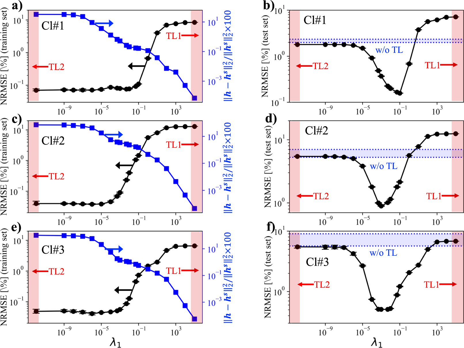
First, given that $ {\lambda}_1 $ serves as a penalty term during the fine-tuning, the NRMSE of the training set generally decreases with a decrease of $ {\lambda}_1 $ for all the clusters. On the other hand, $ \parallel \boldsymbol{h}-{\boldsymbol{h}}^s{\parallel}_2^2 $ / $ \parallel {\boldsymbol{h}}^s{\parallel}_2^2 $ continues to increase as $ {\lambda}_1 $ decreases, indicating that the parameters in the target task become more dissimilar to those in the source task with a decrease of $ {\lambda}_1 $ . This trend demonstrates that the magnitude of $ {\lambda}_1 $ mainly controls the degree of knowledge transfer from the source to the target task.

Second, as the magnitude of $ {\lambda}_1 $ becomes sufficiently large (i.e., >10⁴), $ \boldsymbol{h} $ becomes nearly identical to $ {\boldsymbol{h}}^s $ , illustrating that the transfer learning method for this case is equivalent to TL1, where the knowledge gained from the source task is fully transferred to the target task. In that case, the NRMSE of the test set can be notably higher than the case without applying transfer learning (see Figure 8b and d as an example), indicating that TL1 would play a negative role in predicting the ignition delay of the hydrogen/air mixture for the target task even if the difference in $ {T}_0 $ is relatively small. This would be primarily attributed to the non-linear nature of chemical kinetics, where reaction rates are highly sensitive to temperature change.

Third, as the magnitude of $ {\lambda}_1 $ approaches near zero, the corresponding transfer learning method represents TL2, where the parameters obtained from the source task are used to initialize the parameters in the target task. In this scenario, $ \parallel \boldsymbol{h}-{\boldsymbol{h}}^s{\parallel}_2^2 $ / $ \parallel {\boldsymbol{h}}^s{\parallel}_2^2 $ is relatively high, indicating that the knowledge acquired from the source task is prone to be lost during the fine-tuning process. Nonetheless, it is worth mentioning that the NRMSE of the test set using TL2 nearly equals that obtained from the best ANN model without applying transfer learning. Furthermore, the results of TL2 show less fluctuation from the 10 repetitions of training compared with the results without applying transfer learning. This suggests that initializing the ANN model of the target task with the parameters gained from the source task can be considered an appropriate initialization scheme, provided that the similarity between the source and target tasks is high.

Lastly, the NRMSE of the test set reaches its minimum as the magnitude of $ {\lambda}_1 $ has a finite value (i.e., $ {\lambda}_1= $ $ O $ (10 $ {}^{-4}- $ 10 $ {}^{-1} $ )) for all the clusters. In this case, the resultant NRMSE is approximately an order of magnitude lower than that obtained from training the ANN model from scratch, clearly demonstrating that TL3 with an optimal value of $ {\lambda}_1 $ can remarkably improve the performance of the neural network model for the target task. Note that to achieve a comparable level of NRMSE as that obtained from TL3, the ANN model trained from scratch requires a larger number of $ {N}_{\phi } $ , ranging from 15 to 30, indicating that TL3 can reduce the requisite number of training samples up to eight times. Furthermore, the ANN model training with the use of the optimal value of $ {\lambda}_1 $ is nearly insensitive to the number of training repetitions. This is attributed to the well-known effect of regularization on the stochastic optimization process. Hence, the overall number of training repetitions required to find the optimal ANN model in the target task can be significantly reduced by applying TL3 with an optimal value of $ {\lambda}_1 $ , provided that the source and target tasks are similar in parameter space.

Based on the observations in Figure 8, it can be inferred that the loss function in the target task is likely to contain multiple local minima such that the training result of the ANN model may not reach the global minima of the loss function, especially with the sparse dataset. One method to address this issue and improve the performance of the ANN model is to utilize the pretrained ANN model. If the source and target tasks are similar to each other in the parameter space, then initializing the parameter in the target task ( $ {\boldsymbol{h}}_0 $ ) with that from the source task ( $ {\boldsymbol{h}}^s $ ) can assist in searching for the optimal parameters. Hence, the performance of the ANN model with TL2 has the potential to show better performance compared with the ANN model trained from scratch. Furthermore, TL3 with the optimal value of $ {\lambda}_1 $ can help prevent $ \boldsymbol{h} $ from significantly deviating from $ {\boldsymbol{h}}^s $ during the fine-tuning step, which can enhance the accuracy in predicting $ {\tau}_{\mathrm{ig}} $ in the target task.

Regarding the computational cost for training ANN models, the present study assumes that the number of training samples in the target task is small, resulting in a significantly lower training cost for the target task compared with the source task. For instance, the wall clock time required to train the source task at $ {T}_0 $ = 1050 K with $ {N}_{\phi } $ = 30 is 3150 s for Cl#2, while the wall clock time for training target task for $ {T}_0 $ = 1050 K with $ {N}_{\phi } $ = 4 is 328 s when using TL3 with $ {\lambda}_1={10}^{-4} $ (see Figure S2 in Supplementary Material). This is simply because the number of training samples in the target task is noticeably smaller than that in the source task. Moreover, the convergence rate for training the target task can be further improved if an ANN model trained with a specific $ {\lambda}_1 $ is used as an initial guess for the training of the next ANN model with a different $ {\lambda}_1 $ .

It is also worth mentioning that the computational cost of collecting training samples relative to the cost of performing the sensitivity evaluations by varying $ {\lambda}_1 $ is case-specific and mainly determined by the target configuration. For example, in our previous study, the computational cost for generating training samples accounts for 12.5% of the target 2D DNS run (Jung et al., Reference Jung, Kumar, Echekki and Chen2024), and is expensive compared with the ANN training cost which accounts for $ \sim $ 0.1% of the 2D DNS run. Therefore, the proposed TL approach is particularly useful when the computational cost for obtaining high-fidelity training samples is expensive.

Next, a posteriori evaluation of the PC-transport ROM with different transfer learning strategies is carried out by performing a series of 0D simulations of a hydrogen/air mixture using the PC-transport ROM for the target task, where $ {T}_0 $ = 1050 K and $ {N}_{\phi } $ = 4. Figure 9 shows the variations in $ {\tau}_{\mathrm{ig}} $ as a function of $ \phi $ depending on the different transfer learning methods. The PC-transport ROM fails to predict the overall ignition trend when the ANN is trained from scratch or trained with TL1. Note that the PC-transport ROM with TL1 inaccurately captures the early stage of 0D ignition, leading to error accumulation over time. Consequently, the PC-transport ROM with TL1 fails to undergo a thermal runaway crossing for the full range of $ \phi $ and, hence, $ {\tau}_{\mathrm{ig}} $ approaches infinity.

Figure 9.

Variations in (a) 0D ignition delay time, $ {\tau}_{\mathrm{ig}} $ , predicted by FOM (solid symbol) and PC-transport ROMs trained by applying different transfer learning methods, and (b) the relative-error of the PC-transport ROMs compared with FOM for the homogeneous hydrogen/air mixture with various $ \phi $ at $ {T}_0 $ = 1050 K. $ {N}_{\phi } $ of the training set is set to 4. The values of the optimal $ {\lambda}_1 $ for TL3 are 5 $ \times $ 10 $ {}^{-2} $ , 1 $ \times $ 10 $ {}^{-3} $ , and 1 $ \times $ 10 $ {}^{-3} $ for Cl#1, Cl#2, and Cl#3, respectively. The ROM with TL1 fails to predict ignition, and therefore, the result with TL1 is not shown in the figure.

The overall performance of the PC-transport ROM with TL2 is better than the PC-transport ROM without applying the transfer learning method or with TL1, demonstrating the importance of the initialization scheme and the fine-tuning step on the result, respectively. Here, $ {\tau}_{\mathrm{ig}} $ predicted by the PC-transport ROM with TL2 is in relatively good agreement with that from the FOM when $ \phi $ is near those in the target task training dataset (i.e., $ \phi $ of 0.2, 1.0, 2.0, and 3.0), while the performance of the ANN model decreases as $ \phi $ becomes farther from those in the training dataset of the target task.

For the PC-transport ROM with the optimal value of $ {\lambda}_1 $ (i.e., TL3), it is readily observed that the PC-transport ROM shows a good performance of predicting $ {\tau}_{\mathrm{ig}} $ over a wide range of $ \phi $ . This result substantiates that the regularization-based transfer learning framework can increase the accuracy of the ANN model with the sparse training dataset. Figure 10 presents the temporal evolution of the PCs with four different values of $ \phi $ of 0.15, 0.65, 1.55, and 2.55, predicted by the FOM and the PC-transport ROM with an optimal value of $ {\lambda}_1 $ . Although a slight time lag exists between the FOM and the PC-transport ROM results as $ \phi $ deviates farther from values in the training dataset, the PC-transport ROM can reasonably capture the onset of ignition and the subsequent equilibrium period of the PCs.

Figure 10.

Temporal evolution of the PCs that represent the homogeneous hydrogen/air mixture at $ {T}_0 $ = 1000 K and $ \phi $ of 0.15, 0.65, 1.55, and 2.55, respectively (left to right). Solid line: PCs projected from the FOM result, Dashed line: PC-transport ROM using the optimal $ {\lambda}_1 $ in TL3. The values of the optimal $ {\lambda}_1 $ for TL3 are 5 $ \times $ 10 $ {}^{-2} $ , 1 $ \times $ 10 $ {}^{-3} $ , and 1 $ \times $ 10 $ {}^{-3} $ for Cl#1, Cl#2, and Cl#3, respectively.

4.2. TL1–TL3: parametric study in terms of task similarity and data sparsity

Additional parametric studies are carried out by varying $ {N}_{\phi } $ or increasing $ {T}_0 $ to 1300 and 1400 K. Figure 11 shows $ {\tau}_{\mathrm{ig}} $ as a function of $ \phi $ for the target task with $ {T}_0 $ of 1050 K and decreasing $ {N}_{\phi } $ to 2 and 3 by applying different transfer learning methods. Note that as $ {N}_{\phi } $ decreases to 2 and 3, the training dataset is intended not to cover the entire range of the test dataset (i.e., $ \phi $ = 0.5 and 1.5 for $ {N}_{\phi } $ = 2, and $ \phi $ = 0.5, 1.5, and 2.5 for $ {N}_{\phi } $ = 3) such that there exist several test cases where $ \phi $ is outside of the range of the training dataset (see the highlighted regions in Figure 11). The overall variations in $ {\tau}_{\mathrm{ig}} $ predicted by applying different transfer learning methods show a similar trend regardless of the change of $ {N}_{\phi } $ . The PC-transport ROM with TL1 fails to capture the onset of ignition of the hydrogen/air mixture for the entire range of $ \phi $ , while the results with TL2 show a better performance than those without applying transfer learning. The PC-transport ROM with the optimal value of $ {\lambda}_1 $ in TL3 outperforms all the other models.

Figure 11.

Variations in (top) $ {\tau}_{\mathrm{ig}} $ predicted by FOM (solid symbol) and PC-transport ROMs trained by applying different transfer learning methods, and (bottom) the relative error of the PC-transport ROMs compared with FOM for the homogeneous hydrogen/air mixture with various $ \phi $ at $ {T}_0 $ = 1050 K. Here, $ {N}_{\phi } $ of the training set is (left) 2, and (right) 3, respectively. The highlighted region represents the cases where $ \phi $ is out of the range of the training dataset in the target task. The ROM with TL1 fails to predict ignition, and hence its results are not shown in the figure.

As expected, the accuracy of the PC-transport ROM notably decreases as the target $ \phi $ of the 0D simulation is outside of the range of the training dataset, which is a well-known drawback of machine learning models for extrapolation. Nonetheless, the result of the PC-transport ROM with TL3 shows relatively good performance even for the cases where $ \phi $ is outside of the range of the training set. This result implies that the previous knowledge obtained from the source task helps increase the accuracy of the extrapolation of the ANN model, consistent with previous findings (Humbird et al., Reference Humbird, Peterson, Spears and McClarren2020).

Next, target tasks are considered where $ {T}_0 $ is increased further (i.e., $ {T}_0 $ = 1300, and 1400 K) such that the similarity between source and target tasks decreases. Figure 12 shows the variations in $ {\tau}_{\mathrm{ig}} $ for the hydrogen/air mixture with $ {T}_0 $ of 1300 and 1400 K and $ {N}_{\phi } $ of 4 by using various ANN models with or without applying transfer learning methods. For the cases with $ {T}_0 $ = 1300 K, it is found that the PC-transport ROM with the optimal value of $ {\lambda}_1 $ in TL3 shows a reasonable performance over the entire range of $ \phi $ , while the results without applying transfer learning or with applying TL2 exhibit a noticeable error in predicting ignition of a lean mixture. As $ {T}_0 $ in the target task further increases to 1400 K, on the other hand, the result with TL3 shows only a marginal improvement compared with the other cases. This result demonstrates that the performance of the regularization-based transfer learning method decreases with a decrease in task similarity between source and target tasks.

Figure 12.

Variations in (top) $ {\tau}_{\mathrm{ig}} $ predicted by (solid symbol) FOM and PC-transport ROMs trained by applying different transfer learning methods, and (bottom) the relative error of the PC-transport ROMs compared with FOM for the homogeneous hydrogen/air mixture with various $ \phi $ at (left) $ {T}_0 $ = 1300 K and (right) $ {T}_0 $ = 1400 K.

4.3. PaPIR: unified transfer learning method

Finally, the performance of the unified transfer learning method, PaPIR, in the different target tasks is investigated. As discussed in Section 2.4, the central idea of PaPIR is to control the degree of knowledge transfer from the source to the target task by adjusting the magnitudes of $ {\lambda}_1 $ and $ {\lambda}_2 $ , which are associated with the regularization and initialization of the ANN model in the target task, respectively. Unlike TL3, h $ {}_0 $ in PaPIR can be distributed by either a normal distribution function following the Xavier normal initialization method ( $ {\lambda}_2=0 $ ), or $ {\boldsymbol{h}}^s $ ( $ {\lambda}_2=1.0 $ ), or in between the two ( $ 0<{\lambda}_2<1 $ ). In this regard, the effect of the initialization on the performance of transfer learning can be investigated by varying $ {\lambda}_2 $ in PaPIR.

Figure 13 presents the a priori result of the best achievable NRMSE of $ {\dot{\omega}}_{\psi } $ of the test set for three different target tasks (i.e., $ {T}_0 $ = 1050, 1300, and 1400 K with $ {N}_{\phi } $ of 4) as a function of $ {\lambda}_1 $ and $ {\lambda}_2 $ , conditional on each of the three different clusters. Consistent with the previous results, the best achievable (or minimum) value of NRSME is evaluated by repeating the ANN model training 10 times at a given $ {\lambda}_1 $ and $ {\lambda}_2 $ . As shown in Figure 13a, PaPIR covers all the transfer learning methods discussed in the present study, namely, TL1, TL2, and TL3. In general, the results with TL1 exhibit a large error and increase with an increase of $ {T}_0 $ in the target task. In TL3, there exists an optimal value of $ {\lambda}_1 $ that results in a lower NRMSE than for the results either without applying transfer learning or with TL2.

Figure 13.

Distributions of the best achievable value of NRMSE [%] using PaPIR as a function of $ {\lambda}_1 $ and $ {\lambda}_2 $ for the different test datasets out of 10 repetitions of the ANN model training. The target task is varied ranging from $ {T}_0= $ 1050, 1300, and 1400 K (top to bottom) for Cluster 1, 2, and 3 (left to right) with $ {N}_{\phi } $ of 4.

For the case where task similarity is relatively high (i.e., $ {T}_0=1050 $ K in the target task; see Figure 13a–c), the value of NRMSE is mainly governed by the regularization parameter $ {\lambda}_1 $ , whereas it is largely unaffected by a change of the initialization parameter, $ {\lambda}_2 $ . Since the source and target tasks are similar to each other in this case, the optimal value of $ {\lambda}_1 $ is relatively large (e.g., $ {\lambda}_1 $ = 10 $ {}^{-1} $ in Cl#1). Given that a regularization term serves to convexify the objective function, a relatively large magnitude of $ {\lambda}_1 $ leads the ANN model to be insensitive to a change in the initialization scheme. Consequently, PaPIR does not outperform TL3 when the similarity between source and target tasks is high. The best achievable values of the NRMSE depending on the different transfer learning methods are summarized in Table 3.

Table 3.

Best achievable value of NRMSE [%] by using different transfer learning methods for the test dataset with various $ {T}_0 $ and $ {N}_{\phi }=4 $ , out of 10 repetitions of ANN model training

As $ {T}_0 $ in the target task increases to 1300 K, results with Cl#1 (Figure 13d) show that the NRMSE of the test dataset attains its minimum at a relatively low magnitude of $ {\lambda}_1 $ (= 10 $ {}^{-3} $ ). Although the overall variations of the NRMSE are still mainly governed by $ {\lambda}_1 $ , the NRMSE is no longer invariant to a change of $ {\lambda}_2 $ at the optimal value of $ {\lambda}_1 $ , indicating that $ {\lambda}_2 $ starts to play a role in the optimization of the ANN model. Since the magnitude of the optimal value of $ {\lambda}_1 $ decreases compared with the case with $ {T}_0=1050 $ K, the complexity of the loss function at the optimal value of $ {\lambda}_1 $ increases, and consequently, the training result can be varied with the different initialization schemes. This finding indicates that an initialization scheme becomes important in the framework of transfer learning as the similarity between the source and target tasks becomes relatively low. Note that in Figure 13d, the ANN model exhibits a slightly lower magnitude of NRMSE at $ {\lambda}_2 $ of 0.7 compared with that of 1.0, illustrating the potential advantage of PaPIR over TL3. Readers are referred to Table 3 to quantify the difference of NRMSE between PaPIR and TL3. For the results of Cl#2 and Cl#3, on the other hand, $ {\lambda}_1 $ still plays a major role in determining the best achievable value of NRMSE (see Figure 13e and f). This would be because the decrease of task similarity for these clusters is not as pronounced as for Cl#1.

As $ {T}_0 $ in the target task further increases to 1400 K, it is found that $ {\lambda}_1 $ still shows a dominant effect on the NRSME compared with $ {\lambda}_2 $ , demonstrating that the primary factor of determining the performance of transfer learning is a regularization parameter in general. Nonetheless, there are several cases where the ANN model trained with $ {\lambda}_2<1 $ exhibits a lower magnitude of NRMSE compared with the best candidate obtained from TL3 (see Figure 13g). Note that at $ {T}_0 $ = 1400 K, the ratio of the best achievable NRMSE obtained from PaPIR to TL3 is 0.827, 0.984, and 0.866, for Cl#1, Cl#2, and Cl#3, respectively. This result shows that adjusting the initial values of the parameters in the target task can further enhance the performance of transfer learning in the target task with a sparse dataset, especially when the similarity between source and target tasks is low such that the optimal value of the regularization parameter, $ {\lambda}_1 $ , becomes relatively low.

To further investigate the advantage of PaPIR over other transfer learning methods, especially when the task similarity is relatively low, Figure 14 presents the variations in $ {\tau}_{\mathrm{ig}} $ for a hydrogen/air mixture with $ {T}_0 $ of 1400 K and $ {N}_{\phi } $ of 4, predicted by the FOM and the PC-transport ROMs with different transfer learning methods. This figure clearly shows that $ {\tau}_{\mathrm{ig}} $ predicted by PaPIR shows excellent agreement with that from the FOM over the entire range of $ \phi $ , which is clearly distinct from the other models. Although the relative error obtained from PaPIR is slightly higher than that from TL3 or the PC-transport ROM without applying transfer learning at $ \phi >1 $ , the PC-transport ROM with PaPIR shows a more robust performance for predicting the oxidation process of hydrogen/air mixture over a wide range of $ \phi $ .

Figure 14.

Variations in (top) $ {\tau}_{\mathrm{ig}} $ predicted by the (open symbol) FOM and PC-transport ROMs trained by applying different transfer learning methods, and (b) the relative error of the PC-transport ROMs compared with the FOM for a homogeneous hydrogen/air mixture with various $ \phi $ at $ {T}_0 $ = 1400 K and $ {N}_{\phi } $ = 4.

One may argue that under the data-sparse scenario, the number of test datasets is also likely to be insufficient, rendering it infeasible to find the optimal values of $ {\lambda}_1 $ and $ {\lambda}_2 $ by relying on the test dataset. In future work, a systematic way of estimating the optimal values of those two parameters without relying on a test dataset will be investigated. One practical example would be adopting the L-curve criterion, a well-known heuristic method, to find the optimal regularization parameter without relying on the test dataset (Hansen, Reference Hansen1992). Also as future work, we will compare the performance of different methods that “partially” transfer the knowledge of the pretrained neural network model in the target task. This includes applying Bayesian transfer learning methods (Soriano et al., Reference Soriano, Jung, Echekki, Chen and Khalil2024) or Hessian-based transfer learning methods (Jung et al., Reference Jung, Soriano, Chen and Khalil2024), through which the efficiency of the TL methods will be elucidated in various scenarios.

Note also that the present study effectively assesses the efficiency of TL methods in chemical kinetics, as temperature is a key factor that significantly influences these processes. Regularization-based transfer learning has been successfully demonstrated as a robust algorithm not only in the machine learning community in general but also in combustion systems (e.g., across different equivalence ratios (Soriano et al., Reference Soriano, Jung, Echekki, Chen and Khalil2024) and numerical configurations (Jung et al., Reference Jung, Soriano, Chen and Khalil2024)). Therefore, changes in operating conditions, such as equivalence ratio and pressure, are likely to provide similar insights as those found in the present study. The overall efficiency of TL will be further investigated with large hydrocarbon fuels to elucidate the effect of dimensionality and the complexity of combustion systems on transfer learning.