

1. INTRODUCTION
Simulating the past, present and future state of the Greenland ice sheet is important in the light of the recent rapid changes of the ice sheet and the potential sea-level contribution from a decreasing Greenland ice sheet (e.g. Rignot and others, Reference Rignot, Velicogna, van den, Monaghan and Lenaerts2011; Moon and others, Reference Moon, Joughin, Smith and Howat2012; Shepherd and others, Reference Shepherd2012). This has motivated several modelling efforts investigating the future evolution of the ice sheet (e.g. Bindschadler and others, Reference Bindschadler2013; Goelzer and others, Reference Goelzer2013; Vizcaino and others, Reference Vizcaino2015). Projections of the future evolution of the Greenland ice sheet require initialization of the ice sheet model to represent the present state of the ice sheet (Arthern and Gudmundsson, Reference Arthern and Gudmundsson2010). However, this initialization is a challenging task that adds an additional uncertainty to the projections (Aðalgeirsdóttir and others, Reference Aðalgeirsdóttir2014; Nowicki and others, Reference Nowicki2016). Due to the long response time of the ice sheet, in particular, the temperature field within it, one of the common methods for initializing an ice sheet model is by paleoclimatic spin-ups, i.e. running the ice-sheet model through one, or several, glacial cycles, thereby accounting for the influence of the past climate and evolution of the ice sheet in its present state (Rogozhina and others, Reference Rogozhina, Martinec, Hagedoorn, Thomas and Fleming2011; Goelzer and others, Reference Goelzer2013).
The Holocene climate in Greenland is characterized by an abrupt warming at the glacialinterglacial transition at 11.7 kyr BP, leading to the Holocene climatic optimum at ~8–5 kyr BP when temperatures were 2–3°C higher than the temperatures in the late 20th century, followed by a generally cooling climate trend until the late 20th century, interrupted with shorter climate fluctuations such as the Little Ice Age (Dahl-Jensen and others, Reference Dahl-Jensen1998; Kaufman and others, Reference Kaufman2004; Gkinis and others, Reference Gkinis, Simonsen, Buchardt, White and Vinther2014). Records of stable water isotopes, δ 18O and δD, obtained from deep ice cores are widely used proxies for the past temperature variations across the ice sheet (e.g. Dansgaard, Reference Dansgaard1964; Johnsen and others, Reference Johnsen, Dahl-Jensen, Dansgaard and Gundestrup1995; Cuffey and Clow, Reference Cuffey and Clow1997). These records have therefore been used to derive the climate forcing applied in studies of the past evolution and present state of the ice sheet (e.g. Cuffey and Marshall, Reference Cuffey and Marshall2000; Huybrechts, Reference Huybrechts2002; Tarasov and Peltier, Reference Tarasov and Peltier2003; Greve and others, Reference Greve, Saito and Abe-Ouchi2011). However, the conversion from the isotope records to past temperatures remains a non-trivial task due to several processes, such as seasonality of precipitation events and changes in the conditions of the vapour source regions, affecting the isotopic signal and leading to different sensitivities between δ 18O and temperature for different climate regimes (Jouzel and others, Reference Jouzel1997; Gkinis and others, Reference Gkinis, Simonsen, Buchardt, White and Vinther2014).
One of the most commonly used temperature reconstructions for paleoclimatic initialization of ice-sheet models, used for example by the recent SeaRISE assessment (Bindschadler and others, Reference Bindschadler2013), is based on the δ 18O record from the GReenland Ice core Project (GRIP) (Dansgaard and others, Reference Dansgaard1993; Johnsen and others, Reference Johnsen1997). However, the GRIP δ 18O record does not contain a clear signal of the Holocene climatic optimum due to past elevation changes at the drill site which alter the isotopic signal due to a decrease in the δ 18O values with increasing altitude (Johnsen and Vinther, Reference Johnsen, Vinther and Elias2007; Vinther and others, Reference Vinther2009). Thus, temperature reconstructions derived directly from the isotopic values of the GRIP record would lack the warming in the early Holocene unless these effects are taken into account. By contrast, temperature histories derived from inversions of borehole temperature (Dahl-Jensen and others, Reference Dahl-Jensen1998) and recently from isotope-diffusion studies (Gkinis and others, Reference Gkinis, Simonsen, Buchardt, White and Vinther2014) show a clear signal of the Holocene climatic optimum. The larger temperature signal was also found from the interpretation of the isotopic records of two marginal ice caps, where the proxy record was assumed to be undisturbed by flow and elevation changes (Vinther and others, Reference Vinther2009).
In this study, the effect of five different temperature reconstructions derived from stable water isotope records on the Holocene evolution of the Greenland ice sheet is investigated, particularly focusing on the effect of higher surface temperatures during the early Holocene and the existence of a mid-Holocene minimum in ice-sheet volume. The temperature reconstructions used in our study include reconstructions based on the commonly used GRIP δ 18O record (e.g. Huybrechts, Reference Huybrechts2002), as for example used in the SeaRISE assessment (Bindschadler and others, Reference Bindschadler2013), in addition to more recent ice core based reconstructions where the Holocene climatic optimum is better represented (Vinther and others, Reference Vinther2009; Gkinis and others, Reference Gkinis, Simonsen, Buchardt, White and Vinther2014).
2. METHOD
We use the Parallel Ice-Sheet Model (PISM) (Bueler and Brown, Reference Bueler and Brown2009; the PISM authors, 2016), a three-dimensional (3-D), thermo-mechanically coupled ice-sheet model, to investigate the effect of the different Holocene temperatures reconstructions on the evolution of the Greenland ice sheet. In the PISM model, ice flow is approximated by a weighted average between the two shallow approximations; the Shallow Ice Approximation (SIA) (Hutter, Reference Hutter1983) and the Shallow Shelf Approximation (SSA) (Morland, Reference Morland, van der Veen and Oerlemans1987), thereby allowing an adequate representation of both slow and fast flowing regions, while maintaining low computational costs needed for modelling the ice-sheet evolution on the timescales of millennia (Bueler and Brown, Reference Bueler and Brown2009). Values of flow parameters that determine basal sliding and internal deformation were set to the suggested combination from a study by Aschwanden and others (Reference Aschwanden, Fahnestock and Truffer2016), which uses a Glen flow law exponent equal to 3, but here with the flow law enhancement factor set to E = 3, instead of their suggested value of E = 1.25. Aschwanden and others (Reference Aschwanden, Fahnestock and Truffer2016) selected an enhancement factor of E = 1.25 to obtain the best match to the observed ice flow distribution. Using an enhancement factor of E = 3, we found a better match between the modelled present-day ice-sheet volume and the observed volume, and the ice volume is a key parameter in our study.
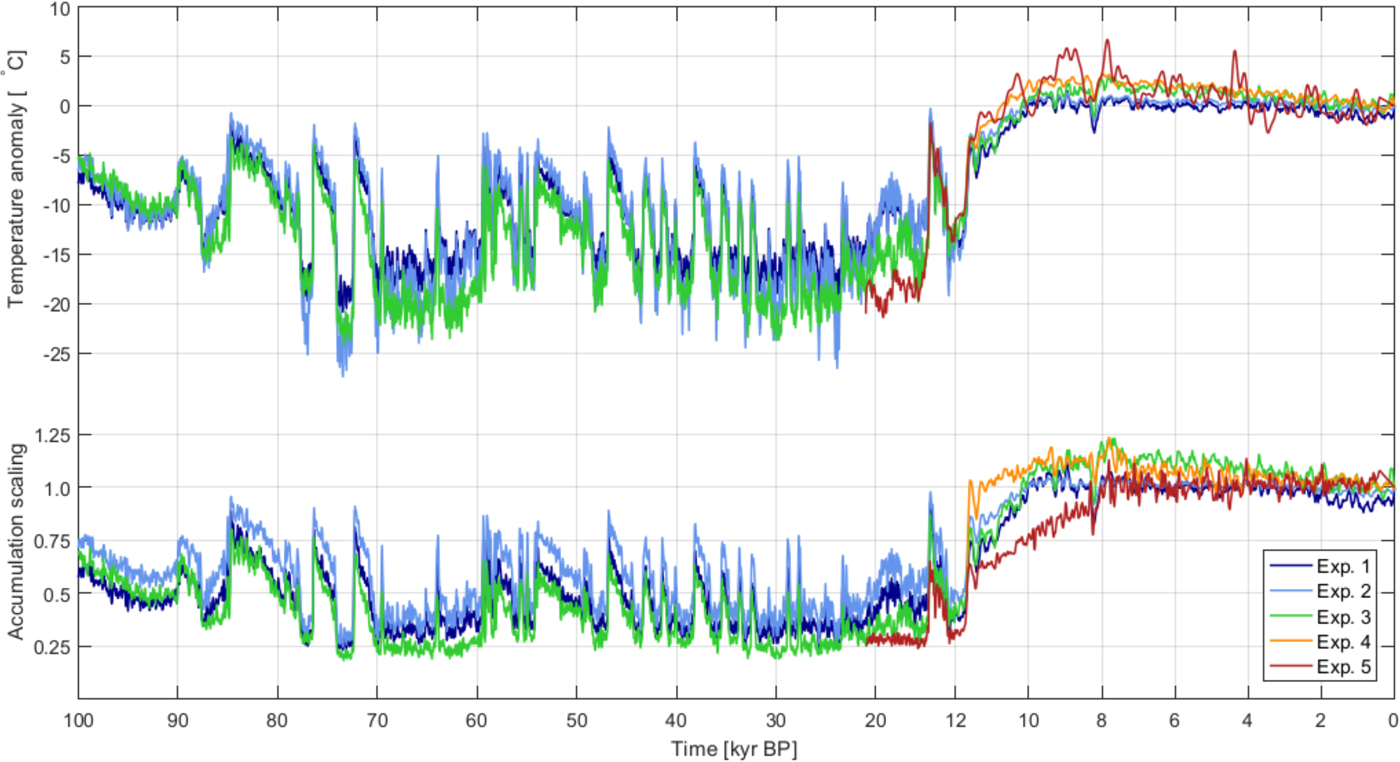
The effect of five different reconstructions of Holocene temperatures and accumulation rates derived from the isotopic records of the GRIP, Agassiz, Renland and the North Greenland Ice core Project (NGRIP) (NGRIP Members, 2004; Vinther and others, Reference Vinther2009) ice cores are assessed by running the ice-sheet model through the last 100 kyr with surface climate prescribed according to the different reconstructions (see Fig. 1). The reconstructions are described in detail below.
Forcing series derived from records of stable water isotopes from the Greenland ice sheet. Top part shows the temperature anomalies (in °C) reconstructed from the δ 18O proxy records using different methods. Note the change in scaling of the x-axis at 12 kyr.The reconstructions based on transfer functions between δ 18O and temperature cover the last glacial and present interglacial and are shown for the 100 kyr used in the simulations (Experiments 1–3). The newer reconstructions based on analysis of δ 18O records from marginal ice caps (Vinther and others, Reference Vinther2009) and on isotope diffusion studies (Gkinis and others, Reference Gkinis, Simonsen, Buchardt, White and Vinther2014) only cover the last 11.7 and 21 kyr, respectively (Experiments 4–5). The lower part shows the scaling of the accumulation rates. The records for Experiments 1–4 are shown with a 100 yr smoothing to illustrate centennial variations.
For the spatial pattern of the climate forcing, we use the average 1960–89 fields of temperature and accumulation rates from the high-resolution regional climate model RACMO2.3 (Noël and others, Reference Noël2015) as the reference present-day surface boundary conditions. These fields are changed according to the reconstructed temperature histories following the approach taken in the SeaRISE assessment (Greve and others, Reference Greve, Saito and Abe-Ouchi2011; Bindschadler and others, Reference Bindschadler2013; Nowicki and others, Reference Nowicki2013), i.e. by adding the temperature anomaly as a uniform off-set, and scaling accumulation rates with a common factor in the entire domain. The mean temperature in the period 1960–89 is thus taken as the present-day temperature, and the temperature reconstructions express the difference from this climate. A constant temperature lapse rate of 5.0°C km−1 is used to account for local changes in ice-sheet surface elevation on the surface temperature during the simulations (Abe-Ouchi and others, Reference Abe-Ouchi, Segawa and Saito2007). Ablation is estimated with a Positive-Degree-Day (PDD) scheme (Reeh, Reference Reeh1991) that applies constant PDD-factors of 8 mm d−1 K−1 for ice and 3 mm d−1 K−1 for snow (mm of water) (Huybrechts, Reference Huybrechts1998; Calov and Greve, Reference Calov and Greve2005). Past changes in sea level are based on the SPECMAP record (Imbrie and others, Reference Imbrie1984).
We use a fixed calving margin set at the present-day coastline, thus the simulated ice sheet cannot expand beyond this. Geological evidences suggest that the Greenland ice sheet had retreated onto the present-day land at ~11 kyr BP for most areas (Funder and others, Reference Funder, Kjeldsen, Kjær, Cofaigh, Ehlers, Gibbard and Hughes2011; Lecavalier and others, Reference Lecavalier2014), and since the focus of the experiments is on the last 10 kyr, we limit the experiments to consider an ice sheet, which has already retreated from the shelf areas to occupy only the present-day land, thus neglecting possible long-term responses from the earlier retreat of the ice sheet.
The present topography of the Greenland ice sheet (Morlighem and others, Reference Morlighem, Rignot, Mouginot, Seroussi and Larour2014) is used to initialize the model at 100 kyr BP and the model is then run through the last 100 kyr by forcing it with the reconstructions of past surface temperatures and accumulation rates as described above. For the first 85 kyr of the simulations, the ice-sheet model is run with a horizontal resolution of 10 km. At 15 kyr BP, the horizontal grid resolution is refined to 5 km. The grid refinement introduces a transient model drift, but over the last 10 kyr, which is the focus of our experiments, the drift is insignificant (<0.5% of the volume).
2.1. Records of past climate
The temperature reconstructions used in this study are derived from stable water isotope records from Greenlandic ice cores. We investigate five different temperature reconstructions for the Holocene, where three of these cover the full spin-up period of 100 kyr, and two cover the last 21 and 11.7 kyr. Of the three climate reconstructions that include the last glacial cycle, covering the last 100 kyr, two are based on the GRIP δ 18O record (Dansgaard and others, Reference Dansgaard1993; Seierstad and others, Reference Seierstad2014) and the third is based on the NGRIP δ 18O record (NGRIP Members, 2004; Seierstad and others, Reference Seierstad2014). These reconstructions are derived directly from the δ 18O of these cores and use transfer functions to convert the δ 18O record to temperature and accumulation rate histories. Two different sets of transfer functions were used, one from Huybrechts (Reference Huybrechts2002) and one from Johnsen and others (Reference Johnsen, Dahl-Jensen, Dansgaard and Gundestrup1995). For the study presented here, we use the recently published age-scale of Seierstad and others (Reference Seierstad2014) that synchronizes the records from three deep ice cores from Greenland as the age-scale of the δ 18O records, thus ages are referred to as before year 2000.
The two last reconstructions use two alternative methods to derive past temperatures from the δ 18O record, which avoids some of the challenges with the transfer function method. These are described below.
The transfer function from Huybrechts (Reference Huybrechts2002) is described in the SeaRISE assessment (Greve and others, Reference Greve, Saito and Abe-Ouchi2011; Bindschadler and others, Reference Bindschadler2013) where it was used to reconstruct a temperature anomaly history from the GRIP δ 18O record. It has a linear δ 18O to temperature relationship and an exponential reduction of accumulation rates according to the temperature anomaly (Huybrechts, Reference Huybrechts2002). This temperature reconstruction is used in Experiment 1.
The transfer functions from Johnsen and others (Reference Johnsen, Dahl-Jensen, Dansgaard and Gundestrup1995) were calibrated using the GRIP bore hole temperature profile. It has a quadratic δ 18O to temperature transfer function and an exponential relationship between δ 18O and accumulation rates. These temperature and accumulation rate reconstructions have been used in Experiment 2. The transfer functions from Johnsen and others (Reference Johnsen, Dahl-Jensen, Dansgaard and Gundestrup1995) result in higher average accumulation rates and larger temperature variations in the glacial period, as well as higher average Holocene temperature, compared with the reconstruction using the transfer function from Huybrechts (Reference Huybrechts2002) for the GRIP δ 18O record (see Fig. 1).
The third temperature reconstruction covering the last 100 kyr is based on the NGRIP δ 18O record. Using the linear δ 18O to temperature transfer function of Huybrechts (Reference Huybrechts2002) as proposed for the GRIP record with the constant term set to the present day δ 18O value of the NGRIP site, the NGRIP δ 18O record is converted into past temperatures anomalies and these are then used to derive an accumulation scaling, also using the transfer function from Huybrechts (Reference Huybrechts2002). This reconstruction is used in Experiment 3. Compared with the forcing based on the GRIP record, this third reconstruction results in colder conditions during the glacial period, and thus more reduced accumulation rates, and has temperatures ~2.5°C above present-day levels during the Holocene climatic optimum (see Fig. 1).
The fourth climate reconstruction used in our study (Experiment 4) is a reconstruction of a common temperature signal in the Holocene of the Greenland region from Vinther and others (Reference Vinther2009), which is based on the δ 18O record from two marginal ice caps, the Agassiz ice cap northwest of Greenland and the Renland ice cap located on the eastern coast of Greenland (Vinther and others, Reference Vinther2009). These two ice caps have not experienced significant changes in surface elevation in this period, thereby simplifying the isotope to temperature conversion from these cores. The reconstruction uses a linear δ 18O to temperature transfer function calibrated using bore hole temperatures from three Greenland ice cores (Vinther and others, Reference Vinther2009). This reconstruction reveals a maximum in surface temperatures in the early Holocene of ~2.5°C (see Fig. 1). Past accumulation rates were derived from annual layer thickness profiles of the three cores used to calibrate the isotope to temperature conversion. For this experiment, we have used the accumulation record derived from the central GRIP location. The result of the spin-up from Experiment 1 at 11.7 kyr BP is used as starting point for this simulation.
The final temperature reconstruction (Experiment 5) is based on a new analysis of the NGRIP δ 18O record and covers the Holocene and the most recent part of the last glacial period. The diffusion of the isotopic signal in the upper layers of the ice column, the firn layer, at the time of deposition is temperature dependent, thereby allowing the temperature history of a site to be reconstructed based on the record of isotope diffusion (Gkinis and others, Reference Gkinis, Simonsen, Buchardt, White and Vinther2014). This technique was used by Gkinis and others (Reference Gkinis, Simonsen, Buchardt, White and Vinther2014) to reconstruct past temperatures for the NGRIP site for the last 21 kyr. The history for past accumulation rates is needed for the analysis, for which they used a reconstruction based on the observed annual layer thickness, thereby allowing for a consistent reconstruction of both the temperature and the accumulation rate histories. This new reconstruction shows colder conditions in the youngest part of the glacial period compared with the histories used in the other experiments and shows temperatures ~4–5°C higher than present during the Holocene climatic optimum (see Fig. 1). This reconstruction extends from 21 kyr BP to 400 yr BP, and it is used in Experiment 5. Beyond 400 yr BP, temperature anomaly and scaling of accumulation rates are assumed to linearly approach zero and one, respectively, at the end of the simulation, thus ending with the present-day climate. The result of the spin-up from Experiment 3 at 21 kyr BP is used as starting point for this simulation.
An additional experiment (Experiment 6) was performed to test the effect of the accumulation rate on the timing of the ice volume variations. Experiment 6 has the same temperature forcing as Experiment 5 from Gkinis and others (Reference Gkinis, Simonsen, Buchardt, White and Vinther2014), but used the accumulation scaling from Experiment 3 based on the NGRIP δ 18O record with accumulation rates derived using the transfer functions of Huybrechts (Reference Huybrechts2002).
The six experiments are summarized in Table 1.
Overview of the temperature and accumulation forcing for the ice-sheet model experiments, and mean forcing temperature anomaly for the last 10 kyr,  $\Delta \bar {T}_{10\,kyr}$. Additional details on model experiment design are given in the text

aHuybrechts (Reference Huybrechts2002).
bJohnsen and others (Reference Johnsen, Dahl-Jensen, Dansgaard and Gundestrup1995).
cVinther and others (Reference Vinther2009).
dThe accumulation rate reconstruction was derived using observed annual layers (λ) and an ice flow model.
eGkinis and others (Reference Gkinis, Simonsen, Buchardt, White and Vinther2014), The temperature reconstruction was derived using an inversion scheme including a firn model, and thus not traditional transfer functions.
Figure 1 shows the forcing series for temperature and accumulation rates applied in the experiments. Comparing the temperature reconstructions of the last 10 kyr, it is clear that the first two experiments based on the GRIP δ 18O have no warming above present-day temperatures during this period. The temperature histories applied in Experiments 3 and 4, derived directly from the NGRIP δ 18O and from the reconstruction based on the analysis of the two marginal ice cores, respectively, have temperatures reaching 2–3°C above present at ~8 kyr BP at the Holocene climatic optimum, slowly declining afterwards.The temperature history applied in Experiment 5 from Gkinis and others (Reference Gkinis, Simonsen, Buchardt, White and Vinther2014), have several short periods of temperatures more than 5°C above present and a warmer climate in the early Holocene, but slightly colder temperatures in the late Holocene.
When comparing the accumulation forcing records used in the different experiments, it is clear that the accumulation rates in Experiments 1–3 are directly related to the δ 18O records through transfer functions, while the accumulation rates in Experiments 4 and 5 are different, particularly in the late part of the glacial period and during the early part of the Holocene.
3. RESULTS
The resulting volume changes of the Greenland ice sheet during the Holocene from the experiments are shown in Figure 2. The six different temperature reconstructions lead to two different characteristic histories of ice-sheet volume during this period. Either (1) continuous volume loss during the Holocene, stabilizing in the last few millennia close to the observed present-day ice sheet volume, or (2) an average negative mass balance in the early Holocene leading to a minimum mid-Holocene ice sheet, followed by a period of a small decreasing positive mass balance on average in the late Holocene, ending in a similar volume of the ice sheet as the other experiments.
Simulated ice sheet volume during the last 12 kyr (in 1015 m3).
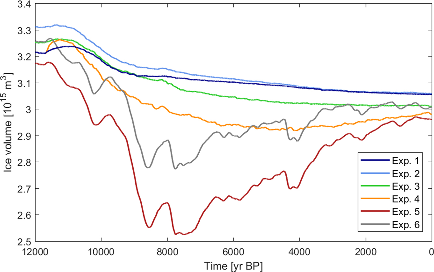
The three experiments with climate forcings derived directly from the isotopic record had the coldest temperatures in the early and mid Holocene (Experiments 1–3), and they all show an ice-sheet history of the first type. In these experiments, the ice sheet has a negative average mass balance through the entire simulation slowly increasing towards zero at the end of the simulation, with a small negative trend of 5–6 Gt yr−1 for the last millennial (see Fig. 3c). The resulting mass loss of the ice sheet during the Holocene corresponds to 5–7% of the final ice-sheet volume in these simulations (see Fig. 2). Between half and two thirds of this volume reduction is accomplished by ~8 kyr BP, ~4 kyr after the onset of the Holocene warming.
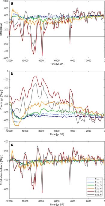
The modelled mass-balance rate (in Gt yr−1) for the ice sheet during the last 12 kyr for Experiments 1–6. (a) Surface mass-balance rate (SMB), (b) discharge rate, and (c) total mass-balance rate calculated as the contribution from SMB, discharge and basal mass balance. All rates are centennial averages for the entire ice sheet and the total mass-balance rate corresponds to the ice volume evolution in Figure 2.
In contrast, in the three simulations where the ice sheet is forced with the temperature reconstructions that have the warmest temperatures during the Holocene climatic optimum (Experiments 4–6), the simulated ice-sheet history is of the second type. The mass balance of the ice sheet is negative on average in the early Holocene, followed by a period of an average positive mass balance as temperatures cool after the Holocene climatic optimum (see Fig. 3c). The initial mass loss in response to the temperature increase in the early Holocene is largest when forcing the ice sheet with the temperature and accumulation reconstructions from Gkinis and others (Reference Gkinis, Simonsen, Buchardt, White and Vinther2014) (Experiment 5). In this simulation, temperature anomalies peak at more than 5°C above the present-day reference climate in the early Holocene and the ice sheet loses 20% of its volume in the 3000 years following the onset of the Holocene through increased surface melting (see Figs 2, 3). As temperatures cool after the Holocene climatic optimum in the later part of the Holocene, the mass balance of the ice sheet becomes positive, and the final volume in Experiment 5 is only 4% smaller than the volume at 12 kyr BP. Additionally, in this experiment the ice volume undergoes variations of 2–3% of the volume at 12 kyr BP on a timescale of several hundred years. These variations are superimposed on the rapid decrease in ice-sheet volume in the early Holocene and a more gradual increase in ice volume in the late Holocene. In the simulation forced with the temperature anomaly from Vinther and others (Reference Vinther2009) (Experiment 4), the same overall pattern of a retreat in the early Holocene followed by a gradual increase in ice volume is observed, although the timing and magnitude differ from Experiment 5 and 6. The minimum ice volume is only ~8% smaller than the volume at the onset of the Holocene and is reached later, at ~4 kyr BP. The ice sheet has a small positive mass balance in the last millennia of this experiment, as discussed further below.
The largest and most rapid retreat of the ice sheet was found for Experiment 5, which was forced by the temperature and accumulation reconstructions of Gkinis and others (Reference Gkinis, Simonsen, Buchardt, White and Vinther2014). In this temperature reconstruction, temperature increases rapidly at the onset of the interglacial and has several shorter periods with temperatures more than 5°C above present in the early Holocene. Their accumulation rates, derived from the layer thickness profile of the NGRIP core, increase slower than the other reconstruction after an initial doubling at the onset of the interglacial, and do not reach present levels until 8 kyr BP (see Fig. 1). This is different from most paleo-climatic simulations of the Greenland ice sheet, where past accumulation rates typically are linked directly to past temperature anomalies (e.g. Huybrechts, Reference Huybrechts2002; Clarke and others, Reference Clarke, Lhomme and Marshall2005; Greve and others, Reference Greve, Saito and Abe-Ouchi2011). To test if this slower increase in accumulation rates affects the early timing of the minimum Holocene ice volume found in this experiment, Experiment 6 was performed with the temperature forcing from Gkinis and others (Reference Gkinis, Simonsen, Buchardt, White and Vinther2014) similar to Experiment 5, but using the accumulation scaling from Experiment 3. Comparing the simulated ice volume with Experiment 5 (Fig. 2), we find that a concomitant increase in temperature and accumulation leads to a smaller mass loss of the ice sheet in the early Holocene, but the timing of the minimum is similar in the two experiments and controlled by the temperature forcing. As the accumulation rates approach the present-day level, the difference between the ice sheet volume decreases, and at the end of the simulation, the volume of the ice sheet in Experiment 6 is only 1% larger than the volume in Experiment 5. Comparison between the experiments shows that a delayed increase in accumulation rates at the onset of the Holocene relative to the increase in surface temperatures as in Experiment 5 can enhance the retreat of the ice sheet, and still have a small influence on the present-day ice sheet volume.
The evolution of ice volume varies in time and the total mass balance rate (in Gt yr−1) is the sum of contribution from the surface mass balance (SMB), the basal mass balance, and discharge to the ocean (see Fig. 3). The two dominating terms of the ice sheet's mass balance are the SMB and ice discharge. The discharge is calculated as the calving flux over a fixed-calving-margin set at the present coastline (the PISM authors, 2016), i.e. discharge may be underestimated when the ice sheet retreats beyond the present coastline. The contribution from the basal mass balance is minor, almost constant in all experiments and in general <5% of the SMB, except in Experiment 5 and 6 at times when the SMB decreases towards zero (see Fig. 3a).
A few centuries after the onset of the Holocene, the average total mass balance of the ice sheet is negative in all five simulations (see Fig. 3c). As the ice sheet adapts to the increased surface temperatures, the mass balance approaches zero for most simulations, though variations of ~20–50 Gt a−1 is observed throughout the simulations. For Experiment 5, the centennial averaged mass balance shows larger variations, ranging between −600 and 300 Gt a−1, reflecting the variations in the temperature forcing and leading to several local minima in the simulated ice volume history.
The modelled discharge rates initially increase for a few thousand years at the onset of the interglacial warming, after which they are only slightly varying for the rest of the simulation in Experiments 1–3. For the simulations with a larger retreat of the ice sheet, the discharge rate is found to decrease with the ice sheet volume and increase again as the ice sheet advances, due to the fixed calving margin at the present-day coastline. Due to this limitation of the model setup, the modelled discharge rates should, therefore, be viewed as a result of inland ice dynamics and not as a driver of dynamics in these simulations.
In the simulations, the SMB is calculated with a PDD-scheme, and it therefore correlates well with the applied temperature forcing. The modelled ice sheets have similar SMB in Experiments 1–3, with a value of ~550–600 Gt yr−1 and with a small positive trend during the last 10 kyr for Experiments 2 and 3, whereas the average SMB in Experiment 1 is almost constant throughout the last 10 kyr of the simulation. The SMB of Experiment 4 has short-term variations similar to the variations in the SMB from Experiments 1–3 with about twice the magnitude. The SMB is ~450 Gt yr−1 in the early Holocene, gradually increasing from the mid-Holocene to reach ~600 Gt yr−1 for the last millennia. In Experiment 5 and 6, the SMB is much more variable than in any of the other experiments and even becomes negative for short periods in the early Holocene, some lasting up to several hundred years, when the temperature forcing anomaly exceeds ~4°C.
Inspection of the spatial pattern of the ice sheet retreat during the Holocene shows that the large mass loss at the margins is partly counterbalanced by ice sheet thickening in the interior (see Fig. 4). Between 12 and 8 kyr BP, the ice sheet retreats from the coast in all five experiments, and up to 200 m increase in ice thickness occurs in the early Holocene in response to the increase in accumulation rates. The extent and magnitude of this thickening depends on the temperature and accumulation forcing. Experiment 5 with highest temperatures in the early Holocene shows a smaller area of thickening compared with the other experiments and has an early and large thinning along the margins, particularly along northern and western margins (Fig. 4). After 8 kyr BP, the general spatial pattern of the thickness change differs for the ice sheets which have a continued decline in ice volume through the Holocene (Experiments 1–3) and those that reach a minimum volume during the early or mid Holocene (Experiments 4–5). For Experiments 1–3, only a modest further increase in ice thickness in the central parts is seen, on the order of a few tens of meters and thinning is progressing towards the interior. For the last few millennia, the ice sheet generally thins and thickness differences are <50 m except for a few areas along the margins (Fig. 4, top row). For Experiments 4 and 5, the marginal ice loss before 8 kyr BP is larger than for the other experiments and the simulated ice sheets thin further into the interior, particularly in the southwest and the north (Fig. 4). In the mid and late Holocene, the two simulations differ. In Experiment 4, a slow widespread thinning of the entire ice sheet continues in the mid Holocene and only in the last few millennia does the ice sheet begin to thicken again in the areas which have thinned the most (Fig. 4, middle row). In Experiment 5, where the temperature forcing is characterized by a very warm early Holocene and a cold late Holocene, the ice sheet has thickened by several hundred meters in the southwest in the mid Holocene as the temperatures cool, but show a further small thinning in the northeast. In the late Holocene, the ice sheet thickens along the margins in most areas, particularly in the northeast and southwest that experienced the largest retreat during the peak warming in the early Holocene (Fig. 4, bottom row).
Ice sheet thickness changes during the early, mid and late Holocene for Experiment 1 (top row), Experiment 4 (middle row) and Experiment 5 (bottom row). Contour lines (in m with 250 m spacing) show ice-sheet surface elevation at the end of each 4 kyr interval and colour scale indicates ice sheet thinning/thickening in meters during the 4 kyr period.

The modelled present-day ice sheet volume match the observed present-day volume within 3% (experiments 1–3) and <0.5% (experiments 4–6). The spatial pattern of the difference between modelled ice thickness and observed ice thickness (Morlighem and others, Reference Morlighem, Rignot, Mouginot, Seroussi and Larour2014) shows a difference of ~100 m to a few hundred meters in the interior with the modelled ice sheet being too thin, and larger differences closer to the margin with the modelled ice sheet being too thick (Fig. 5). Similar differences in topography was found in paleoclimatic studies performed with other ice-sheet models (Greve and others, Reference Greve, Saito and Abe-Ouchi2011; Nowicki and others, Reference Nowicki2013; Peano and others, Reference Peano, Colleoni, Quiquet and Masina2017). The consistent pattern of interior ice being too thin and ice near their margin being too thick suggests that the ice viscosity is too low or amount of basal sliding is too high. Aschwanden and others (Reference Aschwanden, Fahnestock and Truffer2016) selected a combination of optimal model parameters for the PISM model in order to simulate the Greenland ice sheet flow pattern. They tuned the model to match the present-day ice sheet flow pattern, and found a suggested value of the enhancement factor of E = 1.25. However, using their suggested set of model parameters, we found that the modelled present-day ice sheet volume was 16–19% larger than the observed volume. Observations of bore hole deformation show that ice deposited during the last glacial deforms three times faster than Holocene ice in Greenland (Dahl-Jensen, Reference Dahl-Jensen1985; Gundestrup and others, Reference Gundestrup, Dahl-Jsense, Hansen and Kelty1993; Thorsteinsson and others, Reference Thorsteinsson, Waddington, Taylor, Alley and Blankenship1999). This effect changes over time and would imply transient effects on the ice sheet flow and thickness (MacGregor and others, Reference MacGregor2016). The PISM set-up assumes a uniform enhancement factor, and investigations of the effects from a gradually thinning layer of soft glacial ice in the bottom part are not possible here. Following previous Greenland simulations, we used an enhancement factor of E=3 corresponding to glacial ice (e.g. Clarke and others, Reference Clarke, Lhomme and Marshall2005; Aðalgeirsdóttir and others, Reference Aðalgeirsdóttir2014). We kept all other model parameters at the suggested values of Aschwanden and others (Reference Aschwanden, Fahnestock and Truffer2016), and obtained a modelled present-day ice sheet volume in agreement with the observed present-day volume of 7.36 m sea-level equivalent (Bamber and others, Reference Bamber2013). Other parameter combinations may exist, which would result in a similar good fit to the observed volume. Comparison with borehole temperatures show that modelled temperatures are in general slightly too warm, which would also lead to softer ice.
The difference between the modelled and the observed present-day Greenland ice sheet shown for all 6 model experiments (in m), and the observed present-day ice sheet (in m) (Morlighem and others, Reference Morlighem, Rignot, Mouginot, Seroussi and Larour2014). Contour lines (in m with 250 m spacing) show ice-sheet surface elevation.

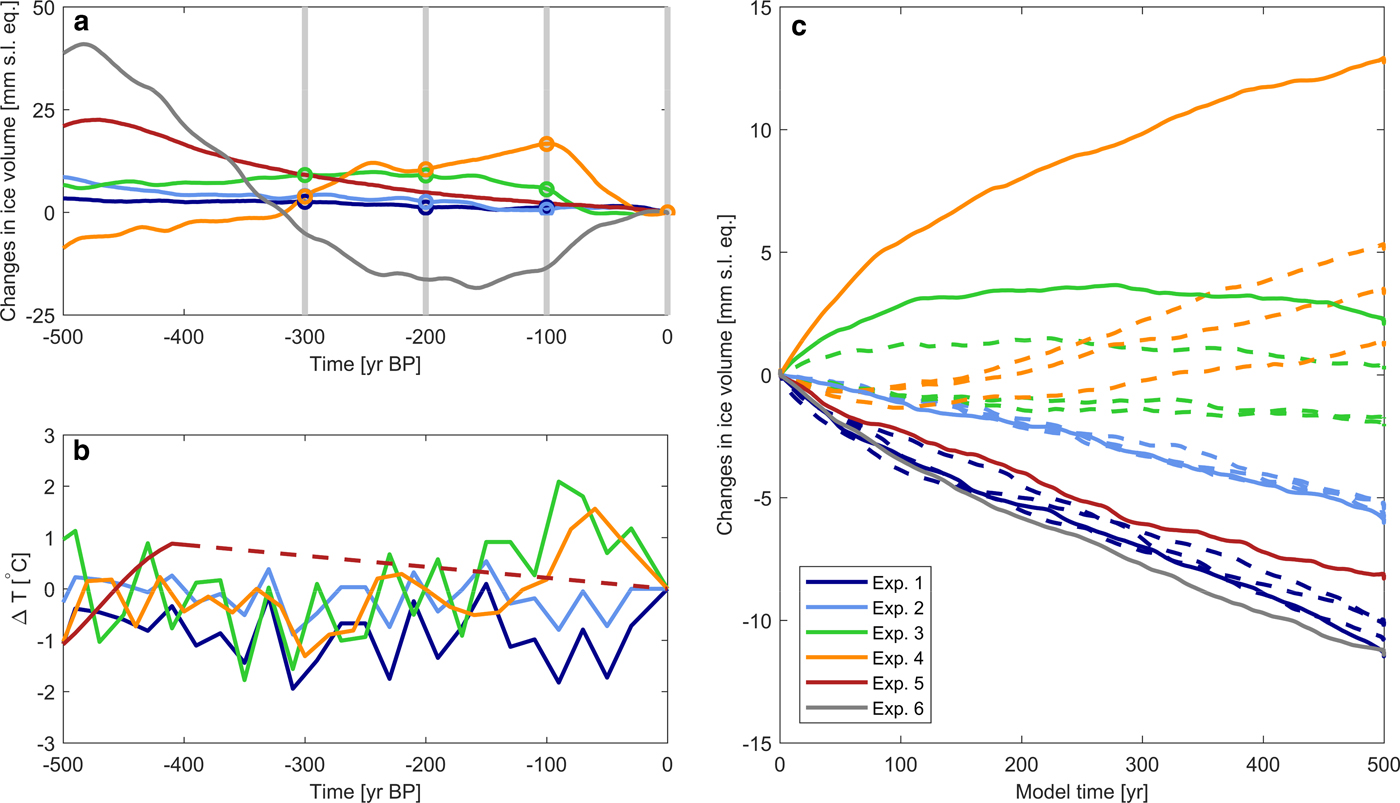
One of the advantages of initializing an ice-sheet model with a paleoclimatic spin-up is that the long-term response of the ice sheet to past climate variations can be accounted for (Goelzer and others, Reference Goelzer2013). As shown in Figure 2, the simulated ice volume of Experiments 1–6 have different trends at present day reflecting their different histories. It is not immediately clear how these millenia-scale trends influence the present and future ice-sheet evolution. In order to investigate the importance of these trends comparedwith shorter-scale trends, we did a set of constant forcing experiments. First, we continued the simulations in Experiment 1–6 for 500 yr under a constant climate forcing. We used the 1960–89 climate forcing as a constant reference present-day climate. The results of these 500 yr constant climate simulations (Fig. 6c) reveal that the modelled ice sheets evolve differently. The ice sheets in Experiment 1, 2, 5 and 6 have a negative mass balance throughout the 500 yr, the ice sheet in Experiment 3 remains at a relatively constant volume, and the ice sheet in Experiment 4 continues to grow during the 500 yr. For the first century, the changes in ice volume are between −0.3 and 0.5 cm sea-level equivalent, i.e. the uncertainty due to the different paleo-climatic reconstructions is ~0.8 cm for the first century. This estimate is similar to the upper range estimate of the uncertainty arising from the initialization methods found by Aðalgeirsdóttir and others (Reference Aðalgeirsdóttir2014), who investigated differences between initialization methods with a constant climate, a paleoclimatic forcing and combined methods. However, the ice sheet is responding to climate on shorter and longer timescales, and recent climate variations on decadal and centennial scales contribute to the present-day trends in addition to the millenia scale trends. In order to perform a crude investigation of the effect from the recent climate forcing, we then did a second set of constant forcing experiments. We performed the same 500 yr constant climate simulations, but starting from the state of the ice sheet at 300, 200 and 100 yr BP. The ice-sheet evolution and climate forcing for the model experiments over the last 500 yr is shown in Figures 6a, b. These additional constant climate simulations were only done for Experiments 1–4, because of the linear extension of the climate forcing for Experiment 5 and 6 for the last 400 yr. Overall, the changes in ice sheet volume during the 500 yr constant climate simulations (Fig. 6c) are smaller than the volume changes seen for the last 500 yr of the paleo-climatic experiments (Fig. 6a). In experiments 1–3, fluctuations in ice volume over the last 500 yr are small, and starting the 500 yr constant climate simulation from earlier model states have only minor influence on the present and future trends (Fig. 6c). The result of Experiment 4 suggests that centennial-scale fluctuations in ice volume have a strong influence on the present and future trends. The increasing trend in the 500 yr constant climate run in Experiment 4 (full line in Fig. 6c) is not observed in the simulations starting at earlier states (dotted lines in Fig. 6c). The difference suggests that the ice-sheet evolution in the first constant climate run in Experiment 4 with an increasing volume is probably mainly a response to the previous 100 yr climate forcing with a negative mass balance, and not a long-term response to the ice-sheet history on millenia scales. Thus the results suggest that the climate forcing of the previous decades to centuries affects the present state of the ice sheet and must be accounted for in simulations of the future evolution.
(a) Ice volume changes (in mm sea-level equivalent) during the last 500 yr of the model experiments. Vertical grey bars indicate additional starting points for model experiments. (b) Temperature anomaly forcing (in °C) for the same 500 yr. (c) Ice volume changes (in mm sea-level equivalent) during the 500 yr constant climate runs starting from present (thick lines). Also shown in (c) are the changes in ice volume (in mm sea-level equivalent) during 500 yr constant climate starting from model states at 300 yr BP, 200 yr BP and 100 yr BP for Experiments 1–4 (dashed lines).
4. DISCUSSION
Geological evidence and studies of the relative sea-level records around Greenland (e.g. Tarasov and Peltier, Reference Tarasov and Peltier2002; Funder and others, Reference Funder, Kjeldsen, Kjær, Cofaigh, Ehlers, Gibbard and Hughes2011; Lecavalier and others, Reference Lecavalier2014) suggest a minimum in ice sheet volume during the mid-Holocene. The results of the simulations presented here suggest that a sustained period of higher than present temperatures in the early Holocene is needed in order to explain the minimum in ice sheet volume in the mid-Holocene. For the simulations forced with temperature reconstructions without a warm early Holocene, the ice sheet retreats continuously throughout the Holocene and reaches a minimum volume at the end of the simulation at present day. The model simulations thus suggest that a temperature forcing containing higher than present temperatures in the early Holocene should be applied in order to obtain a simulated Holocene history of the ice sheet in agreement with the observations.
Geological evidence suggests further that the ice-sheet margins in the southwest retreated up to ~ 100km behind their present-day position during the mid-Holocene (Funder and others, Reference Funder, Kjeldsen, Kjær, Cofaigh, Ehlers, Gibbard and Hughes2011). This evidence is further supported by interpretations of relative sea-level records and bedrock uplift rates that also point towards ice sheet retreat beyond the present ice volume in the mid-Holocene (Khan and others, Reference Khan2008; Funder and others, Reference Funder, Kjeldsen, Kjær, Cofaigh, Ehlers, Gibbard and Hughes2011; Lecavalier and others, Reference Lecavalier2014).
Retreat behind the present-day margin in the southwest for the minimum ice sheet volume is only observed in Experiment 5, where the ice-sheet margin moves 30–60 km further inland than the simulated present-day position. These results are in agreement with the geological evidences which argue for the retreat of similar magnitude in this area (Funder and others, Reference Funder, Kjeldsen, Kjær, Cofaigh, Ehlers, Gibbard and Hughes2011), though the retreat in the simulation is a few millennia too early. It should also be noted that the modelled present-day margin is about 10–40 km too close to the coast in this area. The grid resolution of the ice-sheet model is 5 km, thus these deviations correspond to a few grid points. Finer spatial resolution of the ice sheet model would be needed to support robust estimates of retreat behind the present-day margin in the simulations. The ice sheet is additionally seen to retreat 10–40 km behind the present-day margin in the north for the minimum configuration in both Experiment 4 and 5 (see Fig. 5).
Changes in the spatial pattern of accumulation and temperature arising from forexample changes in ice-sheet topography and other boundary conditions are not directly included when reconstructing the past surface climate of the Greenland Ice sheet using a proxy record from a single site. The proxies reflect the history of local conditions, of which all features, such as interannual variability, might not be transferable to the variability in the large-scale climate. Changes in local conditions due to for example changes in ice-sheet topography or atmospheric conditions would influence the proxies at the site, but all regions of the ice sheet might not experience the same variations at the same time. Nevertheless, ice core records remain one of the most valuable and useful archives for paleoclimatic information of the ice sheets owing to their high temporal resolution and robust chronology (White and others, Reference White2010; Gkinis and others, Reference Gkinis, Simonsen, Buchardt, White and Vinther2014). Studies of isotopic records and borehole temperature profiles from several different sites across Greenland and northern Canada show that all the sites have experienced similar temperature changes on millennial timescales during the Holocene, if the proxy records are corrected for changes in surface elevation of the sites (Vinther and others, Reference Vinther2009). Ice core data thus support our assumption of a constant spatial pattern of climate forcing through the Holocene, which is the focus of our study. Possible transient effects from changes in the spatial patterns during the last glacial or the Holocene climatic optimum (see Fig. 1) are not taken into account in this study.
An alternative approach of reconstructing the past surface boundary conditions for the ice sheet would be to employ a regional climate model as forcing. This method has the clear advantage that changes in spatial patterns can be captured and the important feedbacks between the ice sheet topography and the surface climate, in particular, the SMB, can be accounted for in more detail (e.g. Ridley and others, Reference Ridley, Huybrechts, Gregory and Lowe2005; Vizcaino and others, Reference Vizcaino2015). However, high computational demand still prevents the running of regional climate models at the timescales needed for simulating the evolution of the Greenland ice sheet through an entire interglacial period (Ridley and others, Reference Ridley, Gregory, Huybrechts and Lowe2009). For the experiments presented in this study, we applied a simple PDD-scheme with constant PDD-factors to compute the SMB, rather than applying the SMB field from RACMO. In a PDD-scheme, surface melt is assumed to be proportional to the sum of days with surface temperatures above zero. Thus using a PDD-scheme to estimate SMB has the advantage that the SMB field adapts to the changing topography of the ice sheet, since the surface temperatures for these simulations are corrected by a lapse rate factor to account for changes in ice-sheet surface elevation. Hereby, the feedback between surface elevation and SMB is included in the forcing of the ice-sheet model. However, it should be kept in mind when evaluating the results, that the use of constant PDD-factors and a spatially uniform lapse-rate is likely not representative for all areas of the Greenland region and might differ with time. Also, the detailed spatial pattern of surface melt estimated from a PDD-scheme is different from the present-day field. The SMB calculated from the PDD-scheme is 22% larger than the SMB given by the climate model when forcing the PDD scheme with the reference temperature field, thus surface melt is likely underestimated in the simulations. Sensitivity tests performed for different values of the PDD-factors reveal that the melt pattern is more sensitive to the standard deviation from the yearly cycle, σ (Reeh, Reference Reeh1991), compared with the values of the PDD-factors. An improved fit to the present SMB pattern of the climate model is achieved by adjusting the spatial pattern of σ, though the validity of a given spatial pattern of σ or changes in the PDD-factors for very different climate conditions is not known and we therefore keep the reference values for the PDD-factors and σ. A different representation of this feedback could influence the results, and as the evolution of the ice sheet through most of the Holocene is dominated by surface melt (Lecavalier and others, Reference Lecavalier2014), an improved scheme for estimating the SMB field during the Holocene would be an interesting line of further investigation, but it is beyond the scope of this study.
A recent study by Vizcaino and others (Reference Vizcaino2015) is one of the first to perform a coupled atmosphere-ice-sheet simulation of the Greenland ice sheet through most of the Holocene, thereby assessing changes and feedbacks in the spatial patterns of precipitation, surface temperatures and SMB on the ice-sheet evolution. It is interesting to note that their resulting ice sheet volume history during the last 9 kyr showed a minimum ~4 kyr BP followed by a slow increase to present day, similar to the ice-sheet evolution found in our Experiment 4, which was forced by the temperature reconstruction of Vinther and others (Reference Vinther2009), that has temperatures 2–3°C higher than present during the Holocene climatic optimum. These similarities suggest that the temperature history applied in Experiment 4 is in good agreement with climate modelling during the Holocene.
5. CONCLUSION
In this paper, the effect of forcing an ice-sheet model with several different temperature reconstructions on the Holocene evolution of the Greenland ice sheet is studied. The results show that forcing an ice-sheet model with temperature reconstructions that contain a Holocene climatic optimum that has a sustained period where the temperatures are above present-day values lead to a minimum in ice sheet volume in the early to mid-Holocene. It was further found that applying temperature reconstructions without a Holocene climatic optimum, for example as used in the SeaRISE assessment (Bindschadler and others, Reference Bindschadler2013), leads to a continued mass loss through the Holocene, approaching a steady state in the late Holocene and the smallest ice volume is reached at present day. Our results also indicate that a delayed increase in the accumulation rates in the early Holocene, as suggested by the recent study of Gkinis and others (Reference Gkinis, Simonsen, Buchardt, White and Vinther2014), leads to a larger mass loss in response to the warming at the onset of the Holocene, but only has a minor effect on the simulated present-day ice sheet volume.
The results of these simulations highlight the importance of the temperature reconstruction used to derive climate forcing during a paleoclimatic spin-up. If the purpose is to project future ice loss of the Greenland ice sheet, this forcing can have an influence on the Holocene evolution of the ice sheet and thereby how far from steady state with the present climate the simulated ice sheet is. Although there are several simplifying assumptions in our study that neglect important feedbacks, our results show that a temperature history containing a Holocene climatic optimum leads to a simulated Holocene evolution of the Greenland ice sheet in a better agreement with geological evidences and compares well with previous results of coupled simulations. It is further found that as the simulated ice sheet approaches a steady state at the end of the simulation, the centennial temperature fluctuations become important for the near future evolution of the ice sheet volume.
ACKNOWLEDGMENTS
This work is supported by the Danish National Research Foundation under the Centre for Ice and Climate, University of Copenhagen and Villum Investigator Project IceFlow. Brice Noël and Michiel van den Broeke (IMAU, Utrecht University) are thanked for providing the RACMO2.3 Greenland SMB, precipitation and temperature data. B. Vinther is thanked for providing the Holocene accumulation reconstruction for the GRIP site. We are grateful for computing resources provided by the Danish Center for Climate Computing, a facility build with support of the Danish e-Infrastructure Corporation and the Niels Bohr Institute. Development of PISM is supported by NASA grants NNX13AM16G and NNX13AK27G. We thank the anonymous reviewers and Ralf Greve for their helpful suggestions which substantially improved the paper.


 Open access