


1. Introduction
Radiometric techniques are fundamental to the navigation and tracking of space probes. These techniques include Ranging, Doppler, Delta-Differential One-Way Ranging (Delta-DOR) and Very Long Baseline Interferometry (VLBI). Among these, Doppler tracking is a key component of the Planetary Radio Interferometry and Doppler Experiment (PRIDE), developed by the Joint Institute for VLBI ERIC (JIVE) to provide high-precision spacecraft state vector estimation (Duev et al. Reference Duev, Molera Calvés, Pogrebenko, Gurvits, Cimo and Bocanegra Bahamon2012). Doppler tracking is a method to measure the Doppler shift in radio wave links, enabling the determination of a spacecraft’s radial velocity component. Within the PRIDE framework, Doppler observables have been utilised in various scientific missions, including the study of plasma media (Molera Calvés et al. Reference Molera Calvés2014; Kummamuru et al. Reference Kummamuru2023) and planetary atmospheres (Bocanegra-Bahamón et al. Reference Bocanegra-Bahamón2019).
Between 2013 and 2020, an extensive observing campaign of the European Space Agency’s (ESA) Mars Express (MEX) was conducted to study the interplanetary phase scintillation between the sightlines of Earth and Mars (Kummamuru et al. Reference Kummamuru2023). The primary objective of the long-term campaign was to look at the change electron density as the spacecraft moves through solar conjunction to opposition ( $0-180^{\text{o}}$
elongation). A key feature of the campaign was the large number of telescopes deployed in the observations. These telescopes were employed in ‘three-way’ Doppler tracking observations, which involved transmitting a stable radio signal from a ground-based Deep Space Network (DSN) or European Space Tracking (ESTRACK) antenna to a spacecraft and then receiving the returned signal at different ground-based antennas. The array consists of European VLBI network (EVN) telescopes located in Europe, Asia, and Africa, along with UTAS antennas in Australia. Data from these antennas were used to analyse the link budget, calculate errors in the closed-loop Doppler data, and evaluate the performance of individual telescopes in both VLBI and single-dish mode.
$0-180^{\text{o}}$
elongation). A key feature of the campaign was the large number of telescopes deployed in the observations. These telescopes were employed in ‘three-way’ Doppler tracking observations, which involved transmitting a stable radio signal from a ground-based Deep Space Network (DSN) or European Space Tracking (ESTRACK) antenna to a spacecraft and then receiving the returned signal at different ground-based antennas. The array consists of European VLBI network (EVN) telescopes located in Europe, Asia, and Africa, along with UTAS antennas in Australia. Data from these antennas were used to analyse the link budget, calculate errors in the closed-loop Doppler data, and evaluate the performance of individual telescopes in both VLBI and single-dish mode.
Radiometric techniques are subject to multiple noise elements (Table 1) that affect the quality and precision of data. The most significant of the noise contributions are introduced in the instrumental setup and the propagation path. Instrumental noise arises from a combination of mechanical factors, thermal fluctuations, and variations in frequency standards. Conversely, propagation noises are introduced in media such as the troposphere, ionosphere and interplanetary space. The theory section discusses the instrumental and propagation noise sources in greater detail. The Doppler tracking technique is significantly affected by noise sources in the 1–10 s timescale, which was demonstrated in the analysis of Cassini spacecraft tracking data (Asmar et al. Reference Asmar, Armstrong, Iess and Tortora2005).
The different noise sources and the associated observation technique in which they are observable (Iess et al. Reference Iess, Di Benedetto, James, Mercolino, Simone and Tortora2014; Asmar et al. Reference Asmar, Armstrong, Iess and Tortora2005; Zannoni & Tortora Reference Zannoni and Tortora2013; Tortora et al. Reference Tortora2013).
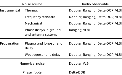
Other noise sources, such as numerical noise and phase ripple, are listed in Table 1. Numerical noise are caused by truncation errors during orbit determination, influenced by factors such as Doppler count time, relative velocity, and mission specifics (Zannoni & Tortora Reference Zannoni and Tortora2013; Iess et al. Reference Iess, Di Benedetto, James, Mercolino, Simone and Tortora2014). Similarly, phase ripple, a dominant error source in classical delta-DOR methods caused by phase dispersion across channels, is mitigated in modern techniques using spread-spectrum signals instead of DOR tones (Towfic et al. Reference Towfic, Voss, Shihabi and Border2019). Source structure noise (Anderson & Xu Reference Anderson and Xu2018) and correlation noise are unique to VLBI which arise from the spatially extend nature of source and cross-correlation inaccuracies respectively. These noise sources are not discussed in detail in this because they are not relevant to Doppler tracking.
Some of the important previous work on the error budget assessment in the Doppler context was done by Bocanegra-Bahamón et al. (Reference Bocanegra-Bahamón, Molera Calvés, Gurvits, Duev, Pogrebenko, Cimò, Dirkx and Rosenblatt2018), who determined the noise budget of MEX in open-loop Doppler residuals from PRIDE stations and closed-loop readings from DSN and ESTRACK antennas. The paper demonstrates how the results of the antennas are comparable in specific scenarios. Asmar et al. (Reference Asmar, Armstrong, Iess and Tortora2005) developed the noise budget of the Doppler tracking observations of the Cassini, achieving Allan deviations close to $10^{-15}$
at 1 000 s integration time. Iess et al. (Reference Iess, Di Benedetto, James, Mercolino, Simone and Tortora2014) advanced this work by consolidating the error budget of the Doppler technique and other radiometric techniques from the Cassini and Rosetta missions for different noise sources. In this work, we aim to determine the noise budget of MEX in closed-loop Doppler residuals from VLBI ground stations. Thus, providing a framework to incorporate local ground stations into radio science experiments and tracking observations beyond the established DSN and ESTRACK networks.
$10^{-15}$
at 1 000 s integration time. Iess et al. (Reference Iess, Di Benedetto, James, Mercolino, Simone and Tortora2014) advanced this work by consolidating the error budget of the Doppler technique and other radiometric techniques from the Cassini and Rosetta missions for different noise sources. In this work, we aim to determine the noise budget of MEX in closed-loop Doppler residuals from VLBI ground stations. Thus, providing a framework to incorporate local ground stations into radio science experiments and tracking observations beyond the established DSN and ESTRACK networks.
The next section provides a mathematical framework for Doppler observables, focusing on their application to system noise characterisation and the development of the noise budget. This is followed by an overview of the campaign’s observational setup. Subsequent sections detail the noise budget and Doppler measurements’ results and analysis, followed by a summary and a discussion.
2. Doppler determination
The processing pipeline of spacecraft Doppler tracking is detailed by Molera Calvés et al. (Reference Molera Calvés, Pogrebenko, Wagner, Cimò, Gurvits, Bocanegra-Bahamón, Duev and Nunes2021), which we briefly describe below. The raw data from different telescopes is initially processed through a Software Spectrometer (SWspec) to compute a time-integrated signal power over the entire band, providing initial detection (signal strength), Doppler shift, and estimation of frequency fluctuations. The next part is the spacecraft tracker (SCtracker) that uses the time series of the initial frequency detections to stop the varying Doppler shift filter out a narrow frequency band. The next processing step is a digital phase-locked loop (dPLL). The dPLL takes the SCtracker output data and performs more precise narrow-band frequency detections by compensating phase rotation. The outputs obtained are the SNR time series, frequency detections, phase, and frequency residuals. These quantities are further used in the noise budget analysis.
The Doppler noise is the measured frequency fluctuations that indicate the variations in the Doppler measurements that interfere with the accurate determination of the spacecraft’s velocity. Given that the Doppler disturbances caused by the Earth’s ionosphere are significantly less intense than those arising from the solar wind, Doppler noise is primarily indicative of the Doppler variations associated with the solar wind (Woo Reference Woo1978). We estimate the Doppler noise by calculating the standard deviation of the spacecraft carrier tone’s residual frequency given by
 \begin{align}F_{r}=F_{\rm det}-F_{\rm fit},\end{align}
where $F_{\rm det}$
is the topocentric frequency detection along the entire frequency band and scan length.
$F_{\rm det}$
is the topocentric frequency detection along the entire frequency band and scan length. $F_{\rm det}$
is determined by calculating the spectral centroid over multiple (5) frequency bins around the spectral peak (Molera Calvés et al. Reference Molera Calvés, Pogrebenko, Wagner, Cimò, Gurvits, Bocanegra-Bahamón, Duev and Nunes2021). The
$F_{\rm det}$
is determined by calculating the spectral centroid over multiple (5) frequency bins around the spectral peak (Molera Calvés et al. Reference Molera Calvés, Pogrebenko, Wagner, Cimò, Gurvits, Bocanegra-Bahamón, Duev and Nunes2021). The $F_{\rm fit}$
is a weighted polynomial fit of the frequency detections to the SNR. A 6th order polynomial fit is used because it best resolves the spacecraft’s carrier tone by effectively removing the dynamical ephemeris variations, leading to a more accurate Doppler compensation.
$F_{\rm fit}$
is a weighted polynomial fit of the frequency detections to the SNR. A 6th order polynomial fit is used because it best resolves the spacecraft’s carrier tone by effectively removing the dynamical ephemeris variations, leading to a more accurate Doppler compensation.
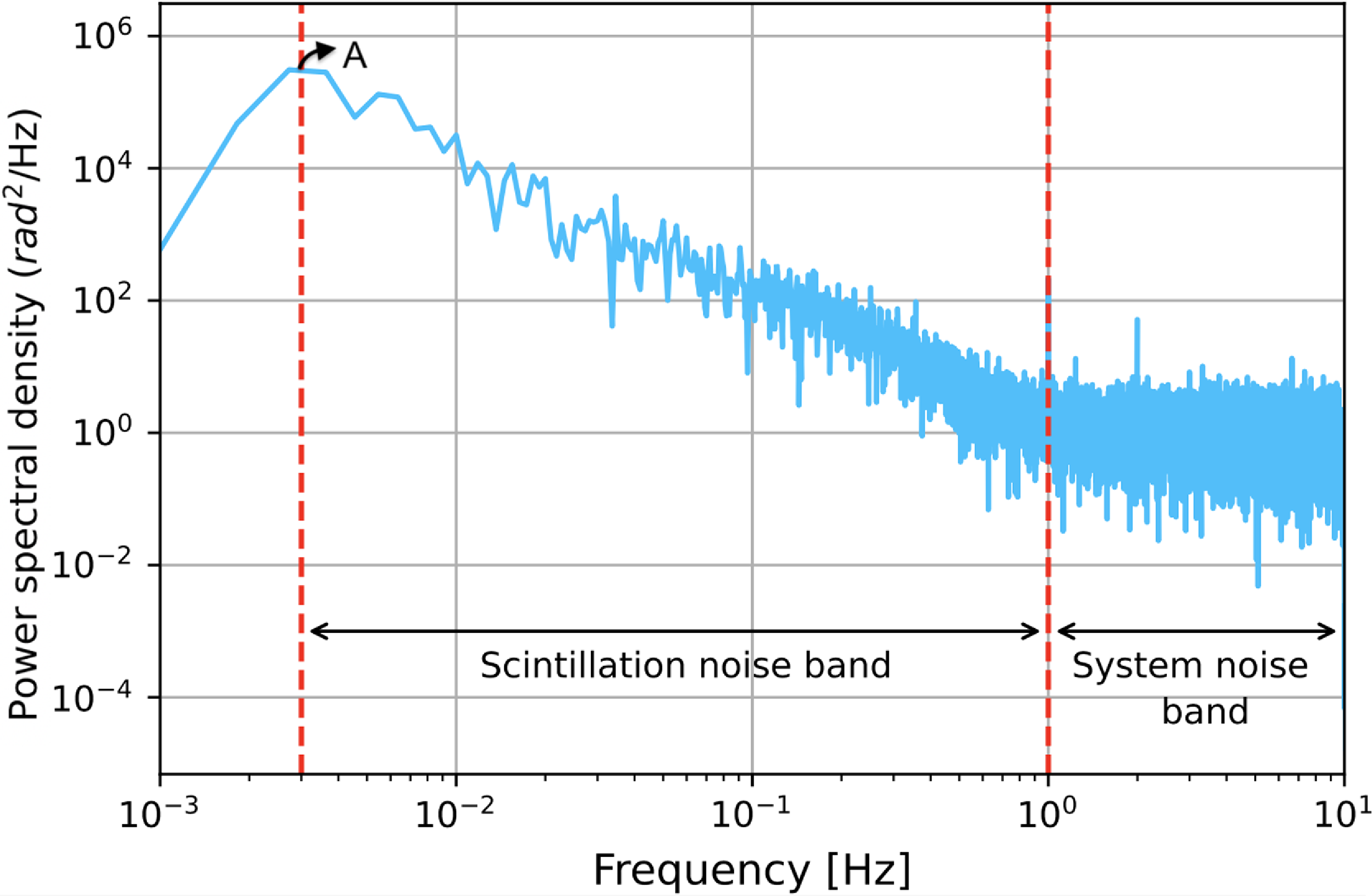
The phase residuals are obtained after processing the signal in narrowband and detail the fluctuations on the phase of the spacecraft carrier signal (Molera Calvés et al. Reference Molera Calvés, Pogrebenko, Wagner, Cimò, Gurvits, Bocanegra-Bahamón, Duev and Nunes2021). These phase residuals are used to construct a frequency domain power spectrum by calculating its fast Fourier transform (FFT) (Fig. 1). The contribution of system noise is expected at higher frequencies, with the cutoff in the spectrum determined via visual inspection. For our observations, the lower end is set as 3 Hz below which the polynomial fitting process filters out low frequency plasma fluctuations. The system phase noise is the root mean square (RMS) of the inverse Fourier transform of the power spectrum values above the cutoff given by
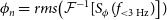 \begin{equation} \phi_{n} = rms\big(\mathcal{F}^{-1}[{S_{\phi}(f_{\lt3\,{\rm Hz}})}\big])\end{equation}
Phase power spectrum from an observation of MEX at Yarragadee on 24 August 2022, with New Norcia Deep Space Antenna as the uplink station. The system noise effects are dominant in the higher frequency region. ‘A’ is the peak power spectral density.
2.1 Doppler noise sources
Doppler tracking is affected by multiple noise sources, as specified in Table 1. The precision of the Doppler is majorly susceptible to instrumental and propagation noises. Instrumental noise arises from the inherent limitations of the signal transmit and receive infrastructure. The mechanical sources are from the physical motion of the antenna’s phase centre, wind loading and irregular thermal expansion of the antenna. The thermal source of instrumental noise is a consequence of the receiver temperature and other temperature-induced fluctuations in the observational pipeline. The noise in frequency standards refers to fluctuations in the stability of the reference signal used for precise tracking, caused by instabilities in the reference clock. As part of analyzing the instrumental noise, we initially look at the performance of individual antennas in terms of their sensitivity. A telescope’s sensitivity can be assessed using its system equivalent flux density (SEFD) value, with lower values indicating a higher sensitivity. The SEFD is calculated using the following equation:
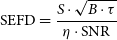 \begin{equation} \text{SEFD} = \frac{S \cdot \sqrt{B\cdot \tau}}{\eta\cdot\text{SNR}}\end{equation}
where S is the received power spectral density, $\eta$
is the antenna beam efficiency, B is the receiver bandwidth and
$\eta$
is the antenna beam efficiency, B is the receiver bandwidth and $\tau$
is the integration time. We have used the measurements collected from our observations to provide a first estimate of the SEFD at the X-band for the participant radio telescope (Table 2).
$\tau$
is the integration time. We have used the measurements collected from our observations to provide a first estimate of the SEFD at the X-band for the participant radio telescope (Table 2).
The sensitivity, size and base noise level for the MEX campaign indicated by the SEFD (X-band), diameter, and system spectral noise level, respectively.
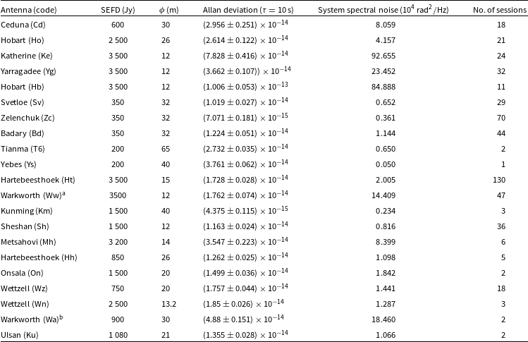
aData credits: Gulyaev, Natusch, & Wilson (Reference Gulyaev, Natusch and Wilson2010).
bData credits: Woodburn et al. (Reference Woodburn, Natusch, Weston, Thomasson, Godwin, Granet and Gulyaev2015).
Phase noise is directly tied to the finite SNR and becomes more pronounced at lower SNR values, reflecting the limitations imposed by signal-to-noise constraints. The one-sided thermal white phase noise spectral density of the received signal gives the relative noise power to the carrier tone, contained in a 1 Hz bandwidth chosen to be centred at a frequency with a large offset from the carrier frequency. The one-sided noise power spectral density (PSD) is used for calculation because the negative frequencies are redundant for real-valued processes, so defining the PSD for positive frequencies is sufficient. We calculate the Allan deviation of the thermal white phase noise using
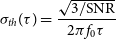 \begin{align} \sigma_{th}(\tau)=\frac{\sqrt{3/\text{SNR}}}{2{\pi}f_{0}\tau} \end{align}
where $f_0$
is the transmission frequency and
$f_0$
is the transmission frequency and $\tau$
is the integration time (Barnes et al. Reference Barnes1971; Rutman & Walls Reference Rutman and Walls1991). Overall, the thermal noise is influenced by the link’s SNR and spanned bandwidth of the observed spectrum, with the SNR depending on factors such as antenna size and SEFD. For the MEX Phobos flyby, the Allan deviation for thermal noise was calculated as
$\tau$
is the integration time (Barnes et al. Reference Barnes1971; Rutman & Walls Reference Rutman and Walls1991). Overall, the thermal noise is influenced by the link’s SNR and spanned bandwidth of the observed spectrum, with the SNR depending on factors such as antenna size and SEFD. For the MEX Phobos flyby, the Allan deviation for thermal noise was calculated as $4.6 \times 10^{-15}$
for
$4.6 \times 10^{-15}$
for $\tau = 10$
s (Bocanegra-Bahamón et al. Reference Bocanegra-Bahamón, Molera Calvés, Gurvits, Duev, Pogrebenko, Cimò, Dirkx and Rosenblatt2018). Another source of instrumental noise is caused by the spacecraft electronics, as observed in the Venus radio occultation experiment (Bocanegra-Bahamón et al. Reference Bocanegra-Bahamón2019), where the Allan deviation was estimated to be approximately
$\tau = 10$
s (Bocanegra-Bahamón et al. Reference Bocanegra-Bahamón, Molera Calvés, Gurvits, Duev, Pogrebenko, Cimò, Dirkx and Rosenblatt2018). Another source of instrumental noise is caused by the spacecraft electronics, as observed in the Venus radio occultation experiment (Bocanegra-Bahamón et al. Reference Bocanegra-Bahamón2019), where the Allan deviation was estimated to be approximately $10^{-13}$
for
$10^{-13}$
for $\tau = 1\,000$
s. In comparison, the Cassini experiment demonstrated an Allan deviation of less than
$\tau = 1\,000$
s. In comparison, the Cassini experiment demonstrated an Allan deviation of less than $3 \times 10^{-16}$
for the same integration time.
$3 \times 10^{-16}$
for the same integration time.
The noise budget must also account for dispersive effects introduced when radio signals propagate through the interplanetary medium, ionosphere, and troposphere. The dispersive effects of plasma in the ionosphere and the interplanetary medium are frequency-dependent. Molera Calvés et al. (Reference Molera Calvés2014), Kummamuru et al. (Reference Kummamuru2023) describe the plasma noise from the Venus Express (VEX) and MEX observations, respectively. The plasma phase scintillation of the radio signal is characterised by performing a first-order approximation of the phase spectrum on a logarithmic scale (Molera Calvés et al. Reference Molera Calvés, Pogrebenko, Wagner, Cimò, Gurvits, Bocanegra-Bahamón, Duev and Nunes2021). The contribution of the solar plasma propagation is dominant between 3 mHz–1 Hz frequencies. Armstrong, Woo, & Estabrook (Reference Armstrong, Woo and Estabrook1979) describe the Allan variance from this segment of the phase power spectrum as
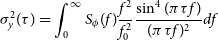 \begin{align} \sigma_{y}^2(\tau)= \int_{0}^\infty S_{\phi}(f)\frac{f^2}{f_{0}^2}\frac{\sin^{4}({\pi{\tau}f})}{(\pi\tau{f})^2}df\end{align}
where f is the spectral frequency and $S_{\phi}(f)$
is the one-sided phase noise spectral density of the received signal.
$S_{\phi}(f)$
is the one-sided phase noise spectral density of the received signal.
The effects of the ionosphere at each station are calibrated using the globally available total vertical electron content (vTEC) maps (Noll Reference Noll2010). The radio link of the deep spacecraft is affected by the tropospheric path delay, too, along the line of sight of observation. The location-dependent wet delay component can be calibrated using the Vienna mapping functions (Böhm,Werl, & Schuh Reference Böhm, Werl and Schuh2006). The wet delay’s non-dispersive and non-homogenous nature necessitates using calibration radiometers (Tortora et al. Reference Tortora2013). More recently, ESA established a tropospheric delay calibration system at the Deep Space Antenna facility in Malargüe, which saw an improvement in 51 $\%$
of the Doppler noise in comparison to the standard global navigation satellite system (GNSS) calibrations (Manghi et al. Reference Manghi2023).
$\%$
of the Doppler noise in comparison to the standard global navigation satellite system (GNSS) calibrations (Manghi et al. Reference Manghi2023).
The phase power is dependent on the solar elongation. A lower solar elongation angle would intensify the mean power spectral density (PSD). The Allan variance of the plasma propagation noise follows through from Equation (5) and is estimated as
 \begin{equation} \sigma_{y}^2(\tau)= \frac{A{\tau}^m}{{\pi}^2{f_0}^2{\tau}^3} \int_{0}^\infty \frac{\sin^{4}({\pi}z)}{z^m}dz \end{equation}
 \begin{equation*}S_{\phi}(f)=\frac{A}{f^m},\end{equation*}
where A is the peak of the PSD, $\tau$
is the integration time, m is the slope of the linear fit.
$\tau$
is the integration time, m is the slope of the linear fit.
In Doppler tracking, frequency standards are crucial for providing precise calibration frequencies. H-masers demonstrate stabilities between $2\times{10^{-15}}$
and
$2\times{10^{-15}}$
and $6.69\times{10^{-16}}$
at 1 000 s integration, enhancing precision in space science (Dai et al. Reference Dai, Liu, Cai, Chen and Li2022). In this case, the ground station frequency reference sources generally have thermal stability in the range of
$6.69\times{10^{-16}}$
at 1 000 s integration, enhancing precision in space science (Dai et al. Reference Dai, Liu, Cai, Chen and Li2022). In this case, the ground station frequency reference sources generally have thermal stability in the range of $10^{-15}$
–
$10^{-15}$
– $10^{-16}$
.
$10^{-16}$
.
3. Observational setup
The MEX campaign (2013–2020) was carried out using 21 different VLBI telescopes across the globe with over 300 observation epochs. During this campaign, the X-band (8.4 GHz) telemetry carrier signal from MEX was observed. The coherent signal was tracked in a closed-loop receiver setting. The closed-loop receiver actively tracked the MEX signal by continuously adjusting its local oscillator to maintain a phase-locked loop (PLL). Raw data is recorded as the broadband radio signal in VLBI Data Interchange Format (VDIF). In addition to the nominal campaign, we conducted ad-hoc observations of MEX in 2023 with co-located telescopes. Each session was segmented into 19-min length scans with a 1-min slewing window for readjusting its position to track the spacecraft between each of them. The analysed data can be segregated into Doppler observables and system noise-based quantities. In the following sections, we shall see how different scenarios help evaluate these variables to assess the performance of telescopes.
The infrastructure of each antenna is characterised by several distinct features. One of the most notable differences is the antenna aperture size, which ranged from the smallest 12-m telescopes operated by UTAS to the largest 65-m telescope in Tianma (Table 2). The telescopes used also differ in that they have either circular or linearly polarised feeds. Deep spacecraft communication is usually done with circular polarization signals to mitigate signal degradation caused by the rotation of the spacecraft or polarization mismatches due to the signal’s passage through the ionised medium.
4. Results and analysis
This section details the instrumental noise budget, system stability, Doppler noise variations, the use of co-located telescopes, and the propagation noise budget. By systematically analyzing the performance of telescopes used in the campaign, we aim to understand the factors influencing the accuracy of Doppler tracking in the context of PRIDE experiments.
4.1 Instrumental noise budget and system stability
The investigation begins with assessing the instrumental noise budget and system stability, which are crucial to evaluating the telescopes’ performance. The SEFD values and Allan deviation quantitatively measure each telescope’s sensitivity and frequency stability, respectively.
The SEFD values and Allan deviation, calculated using Equations (3) and (4), respectively, are listed in Table 2 for the telescopes ranging between 12 to 65 m in diameter. Telescopes such as Hobart and Katherine with higher SEFD values, i.e., poor sensitivity, have lesser frequency stability. On the other hand, large antennas like Kunming (40 m) and Tianma (65 m) present better Allan deviation, partly due to better sensitivity and larger size.
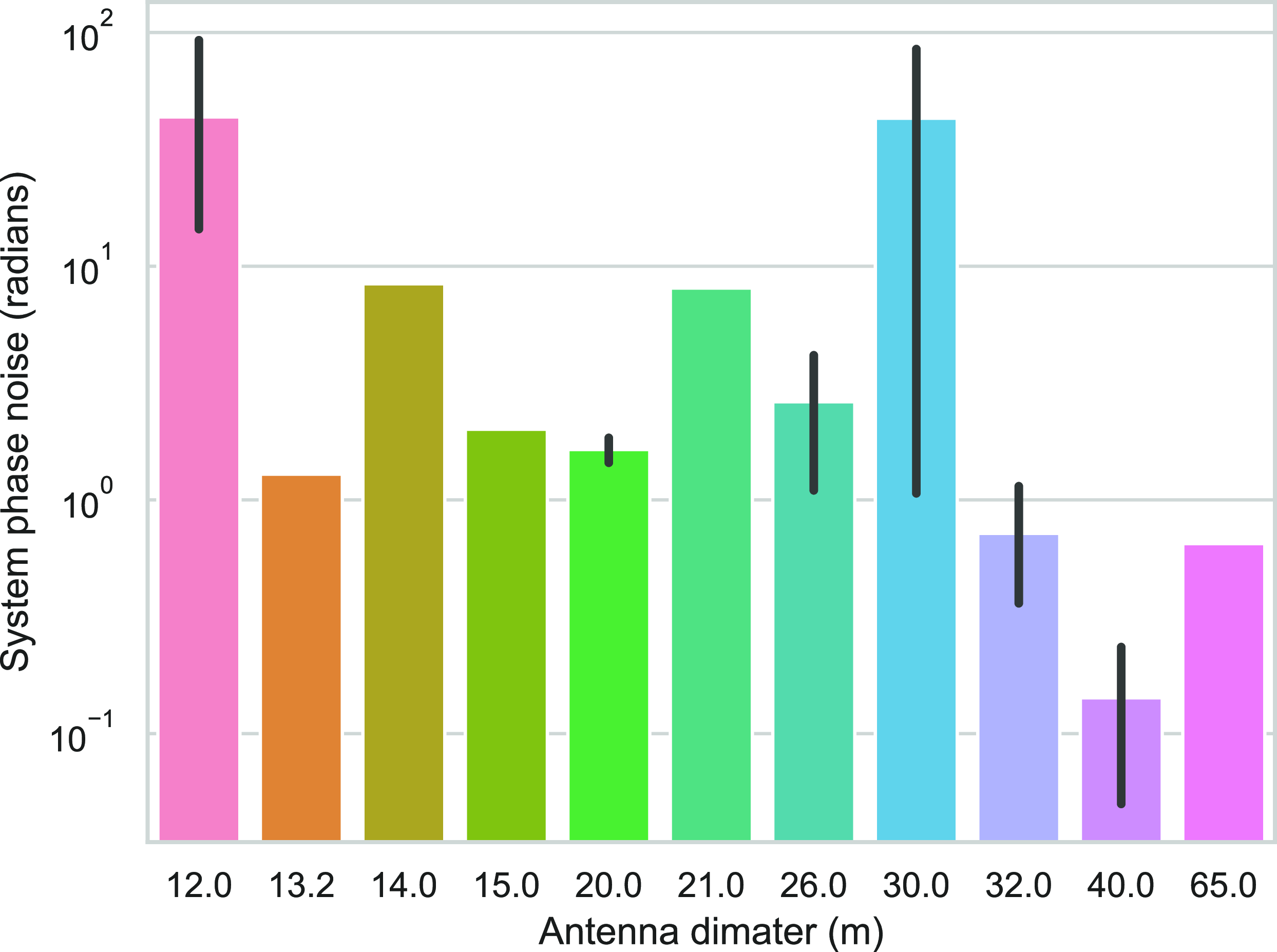
The telescopes’ system phase spectral noise levels are examined to understand their performance during Doppler tracking. The system phase noise is a cumulative result of mechanical vibrations, antenna mount movements, oscillator fluctuations, amplifier inconsistencies, receiver instabilities, and thermal fluctuations. At lower solar elongations, the solar plasma propagation effect saturates the system noise, making it increasingly challenging to assess intrinsic system performance. We select only sessions with solar elongations above 20 degrees to avoid this bias and calculate their system phase spectral noise. Fig. 2 provides an overview of the spectral noise for different-sized telescopes used in the campaign (Kummamuru et al. Reference Kummamuru2023). The assessment shows how Hobart (12 m), Katherine (12 m), and Warkworth (13.2 m) exhibit higher phase noise levels contributed by antenna-based characteristics. We observe a higher level of uncertainty of $\pm0.53\times10^{-14}$
in Hobart’s (12 m) sensitivity, which is likely a result of the increased sensitivity that could be caused by increased receiver temperature or inherent characteristics and noise contributions from the backend signal processing system. The larger telescopes with better sensitivity, like Tianma (65 m) and Kunming (40 m), have lower levels of system phase noise.
$\pm0.53\times10^{-14}$
in Hobart’s (12 m) sensitivity, which is likely a result of the increased sensitivity that could be caused by increased receiver temperature or inherent characteristics and noise contributions from the backend signal processing system. The larger telescopes with better sensitivity, like Tianma (65 m) and Kunming (40 m), have lower levels of system phase noise.
A comparison of the system noise levels obtained from the phase power spectrum with the corresponding antenna sizes. The black lines correspond to the standard deviation for the scenarios when when there were multiple telescopes with the same diameter.
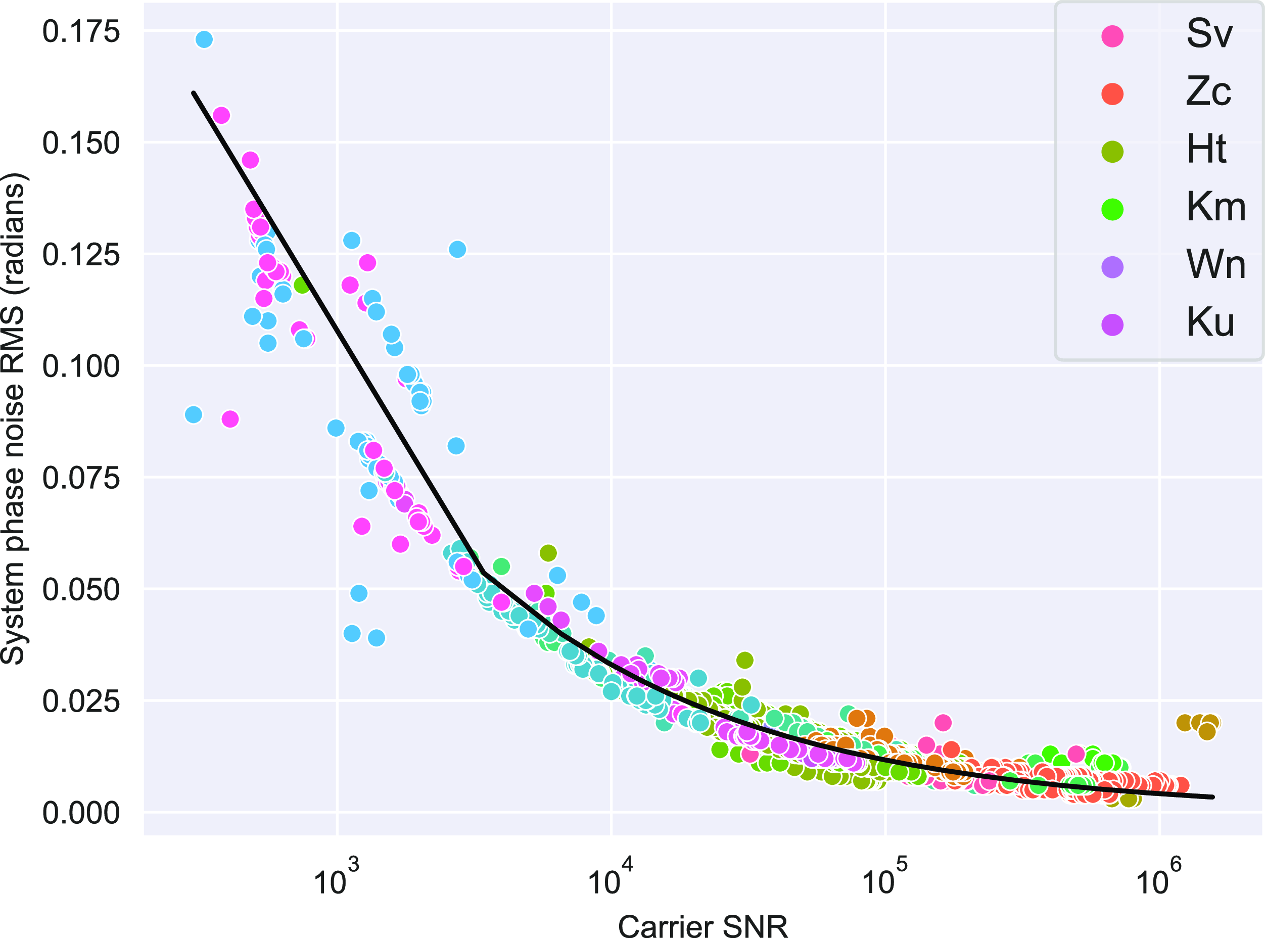
In Fig. 3, the system phase noise obtained from the residual phase is compared as a function of the SNR. It exhibits a decaying relationship between system phase noise RMS ( $\sigma_{\rm phn}$
) and carrier SNR. The linear fit (black line) in the linear-log graph suggests a power-law relationship between the system phase noise and SNR, which approximately follows
$\sigma_{\rm phn}$
) and carrier SNR. The linear fit (black line) in the linear-log graph suggests a power-law relationship between the system phase noise and SNR, which approximately follows $\text{SNR}\propto{\sigma_{\rm phn}}^n$
relation where
$\text{SNR}\propto{\sigma_{\rm phn}}^n$
relation where $n\approx0.5$
. This decaying trend is consistently observed across the different stations, with only certain station-specific variations that could stem from intrinsic factors such as equipment characteristics. Greater sensitivity to noise causes outliers at lower SNR values. The overall analysis indicates that noise can be reduced by improving the system’s sensitivity. This can be achieved through factors such as using larger antennas, lowering the SEFD, or enhancing receiver performance. Additionally, increasing the signal-to-noise ratio (SNR) effectively reduces system phase noise up to a certain threshold, beyond which the system’s inherent noise characteristics dominate. At lower SNR values, the system phase noise is largely dominated by thermal noise and instrumental fluctuations, leading to a nearly linear dependence, where increased SNR directly improves the phase stability as seen in Fig. 3. However, as the SNR continues to increase, the influence of phase instabilities due to propagation fluctuations begin to dominate. These effects introduce a nonlinear saturation in the phase noise behavior, resulting in the observed curvature. Essentially, once the system reaches its intrinsic noise floor, further increases in SNR no longer yield proportional improvements in phase stability. At lower SNR values, the system phase noise is largely dominated by thermal noise and instrumental fluctuations, leading to a nearly linear dependence, where increased SNR directly improves the phase stability. However, as the SNR continues to increase, the influence of external noise sources diminishes, and systematic effects such as phase instabilities, tropospheric and ionospheric fluctuations, and instrumental phase noise begin to dominate. These effects introduce a nonlinear saturation in the phase noise behavior, resulting in the observed curvature. Essentially, once the system reaches its intrinsic noise floor, further increases in SNR no longer yield proportional improvements in phase stability, causing the curve to bend rather than continue linearly.
$n\approx0.5$
. This decaying trend is consistently observed across the different stations, with only certain station-specific variations that could stem from intrinsic factors such as equipment characteristics. Greater sensitivity to noise causes outliers at lower SNR values. The overall analysis indicates that noise can be reduced by improving the system’s sensitivity. This can be achieved through factors such as using larger antennas, lowering the SEFD, or enhancing receiver performance. Additionally, increasing the signal-to-noise ratio (SNR) effectively reduces system phase noise up to a certain threshold, beyond which the system’s inherent noise characteristics dominate. At lower SNR values, the system phase noise is largely dominated by thermal noise and instrumental fluctuations, leading to a nearly linear dependence, where increased SNR directly improves the phase stability as seen in Fig. 3. However, as the SNR continues to increase, the influence of phase instabilities due to propagation fluctuations begin to dominate. These effects introduce a nonlinear saturation in the phase noise behavior, resulting in the observed curvature. Essentially, once the system reaches its intrinsic noise floor, further increases in SNR no longer yield proportional improvements in phase stability. At lower SNR values, the system phase noise is largely dominated by thermal noise and instrumental fluctuations, leading to a nearly linear dependence, where increased SNR directly improves the phase stability. However, as the SNR continues to increase, the influence of external noise sources diminishes, and systematic effects such as phase instabilities, tropospheric and ionospheric fluctuations, and instrumental phase noise begin to dominate. These effects introduce a nonlinear saturation in the phase noise behavior, resulting in the observed curvature. Essentially, once the system reaches its intrinsic noise floor, further increases in SNR no longer yield proportional improvements in phase stability, causing the curve to bend rather than continue linearly.
A comparison of how the system phase noise varies with the mean carrier signal SNR throughout the campaign.
The analysis of system phase spectral noise for the stations Hb and Ke for the periods 2013–2016 and 2020–2021 reveals notable differences. In the 2013–2016 period, only the Ke station had recorded sessions, with an average system phase noise of 6.03 radians for a mean solar elongation of 26.97 degrees. The Hb station had no sessions during this period. In contrast, during the 2020–2021 period, both Hb and Ke stations exhibited significantly higher system phase noise levels. The Hb station recorded an average spectral noise of $80.58\times10^4 {\text{rad}^2}/{\text{Hz}}$
with a mean solar elongation of 84.53 degrees during this period, while the Ke station showed an even higher average system phase noise of
$80.58\times10^4 {\text{rad}^2}/{\text{Hz}}$
with a mean solar elongation of 84.53 degrees during this period, while the Ke station showed an even higher average system phase noise of $109.89\times10^4 {\text{rad}^2}/{\text{Hz}}$
with a mean solar elongation of 86.62 degrees. This highlights a considerable increase in system phase noise post-2020. During this period, the legacy VLBI (S/X) system was being upgraded to the broadband VLBI Global Observing System (VGOS), and the increased system noise can likely be attributed to synchronization offsets in the newly installed Digital Base Band Converter (DBBC). The DBBC is a key component of VLBI receiving systems, performing data acquisition, channel selection, and baseband conversion by applying sampling, filtering, quantization, and FFTs to the input analog signal (Tuccari Reference Tuccari2003). To put into perspective, geodetic observations have a higher tolerance of DBBC noise compared to spacecraft observations on account of having more bandwidth. Another possible explanation could be losses due to the antennas recording in linear polarization, while MEX’s radio echo signal is transmitted in circular polarization along both left and right directions (Pätzold et al. Reference Pätzold2004), leading to signal loss in one direction.
$109.89\times10^4 {\text{rad}^2}/{\text{Hz}}$
with a mean solar elongation of 86.62 degrees. This highlights a considerable increase in system phase noise post-2020. During this period, the legacy VLBI (S/X) system was being upgraded to the broadband VLBI Global Observing System (VGOS), and the increased system noise can likely be attributed to synchronization offsets in the newly installed Digital Base Band Converter (DBBC). The DBBC is a key component of VLBI receiving systems, performing data acquisition, channel selection, and baseband conversion by applying sampling, filtering, quantization, and FFTs to the input analog signal (Tuccari Reference Tuccari2003). To put into perspective, geodetic observations have a higher tolerance of DBBC noise compared to spacecraft observations on account of having more bandwidth. Another possible explanation could be losses due to the antennas recording in linear polarization, while MEX’s radio echo signal is transmitted in circular polarization along both left and right directions (Pätzold et al. Reference Pätzold2004), leading to signal loss in one direction.
4.2 Doppler noise variations in sequential topocentric detections
The Doppler noise is estimated at multiple stages during the data processing (Molera Calvés et al. Reference Molera Calvés, Pogrebenko, Wagner, Cimò, Gurvits, Bocanegra-Bahamón, Duev and Nunes2021). The first instance occurs after the polynomial fitting in SWspec, where the topocentric frequency detections are obtained along with the associated stochastic noise of the polynomial, referred to as ‘DNoise0’. The second instance arises after the dPLL processing, which generates refined topocentric frequency detections and their corresponding stochastic noise, labelled ‘DNoise2’. At this stage, the data is filtered to a 20 Hz bandwidth. Additionally, the stochastic noise of the polynomial fit for the frequency detections generated by SCtracker is termed ‘DNoise1’. However, DNoise1 is not used for our study, as the final dPLL narrowband results are preferred over the SCtracker wideband outputs. As such, our focus remains on DNoise0 and DNoise2 parameters in this study.
4.2.1 Antenna aperture size
To compare how the aperture sizes of the antennas affect DNoise0 and DNoise2, we select sessions where multiple antennas were used, and the solar elongation was sufficiently high ( $\approx63^{\text{o}}$
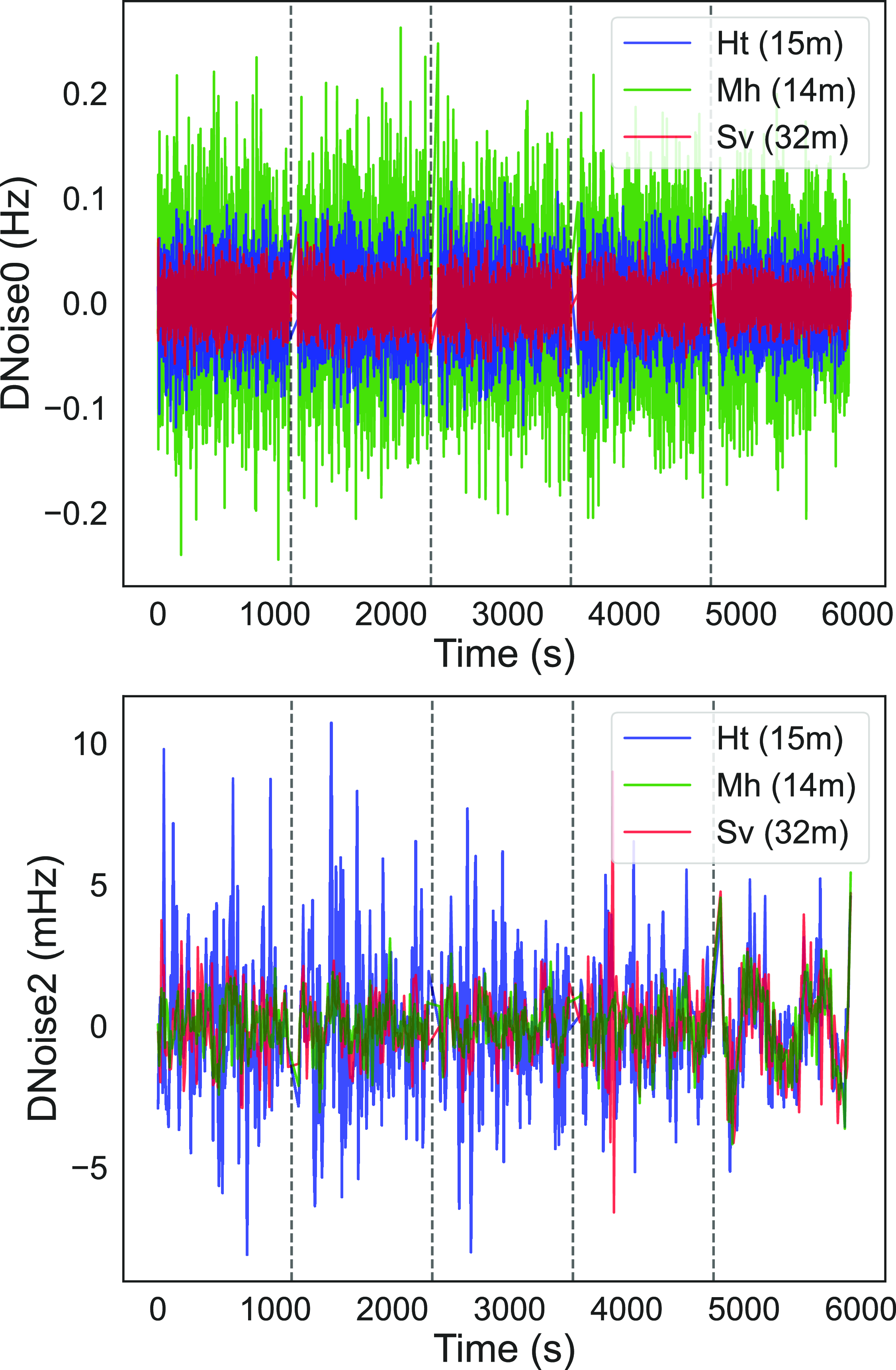
) to minimise the influence of coronal effects. The most suitable was a session on 13 December 2015 involving three antennas of different sizes: Sv (32 m), Ht (15 m), and Mh (14 m). The results in Fig. 4 demonstrates how the aperture size affects the stochastic noise of the initial detection polynomial fit (DNoise0). Specifically, the RMS DNoise0 values in Hz are as follows: 0.0340 for Ht (15 m), 0.0657 for Mh (14 m), and 0.0183 for Sv (32 m). These values highlight that larger antennas exhibit lower DNoise0, with the Sv antenna achieving the lowest noise.
$\approx63^{\text{o}}$
) to minimise the influence of coronal effects. The most suitable was a session on 13 December 2015 involving three antennas of different sizes: Sv (32 m), Ht (15 m), and Mh (14 m). The results in Fig. 4 demonstrates how the aperture size affects the stochastic noise of the initial detection polynomial fit (DNoise0). Specifically, the RMS DNoise0 values in Hz are as follows: 0.0340 for Ht (15 m), 0.0657 for Mh (14 m), and 0.0183 for Sv (32 m). These values highlight that larger antennas exhibit lower DNoise0, with the Sv antenna achieving the lowest noise.
A comparison of Doppler noise levels (DNoise0-top, DNoise2-bottom) between Ht (15 m), Mh (14 m) and Sv (32 m) for a session held on 13 December 2015. The vertical black dotted lines demarcate each scan of 1 140 s length. The RMS values of the DNoise0 for the Ht, Mh and Sv are 0.034, 0.066, and 0.018 Hz, while the DNoise2 values are 2.51, 1.05 and 1.33 MHz, respectively.
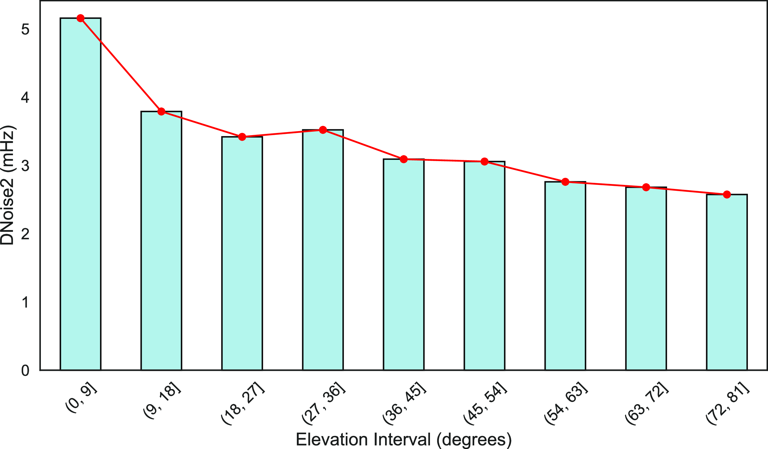
A comparison of how Doppler noise levels (DNoise2) vary at elevation angles across the observing campaign for all stations. The elevation angle is used to represent the average position of the spacecraft during a scan. This means that the antenna is fixed at the position where the spacecraft is anticipated to be at the midpoint of the scan, which occurs 10 min into a total scan duration of 19 min.
In contrast, the differences in the stochastic noise of the fit for the narrowband detection (DNoise2) are much smaller overall, with a maximum difference of 1.4 mHz, indicating that the narrowband processing copes with weaker signals of smaller antennas and extracts frequency detections as accurate as that of the larger antennas. This is expected as the dPLL performs more precise frequency detections in a narrow band by compensating for residual phase rotation. The dPLL mitigates much of the variability seen in the wideband polynomial fit stage (DNoise0). Consequently, the influence of antenna size is reduced in this stage, as the dPLL focuses on refining the frequency detection within a constrained band where systematic noise sources dominate over size-dependent effects.
4.2.2 Elevation angle
The elevation angle is the third parameter evaluated, particularly with tropospheric effects expected to dominate at lower elevations. The DNoise2 variation with the elevation angles for all the sessions across the observation campaign is plotted in Fig. 5. We excluded sessions that were below 20 degrees of solar elongation to prevent any bias in values caused by the proximity of the Sun. The DNoise2 is the highest in the 0-9 degrees elevation range, suggesting stronger tropospheric effects when the target is at a lower elevation. As the elevation angle increases past 9 degrees, a sharp drop is seen in the DNoise2 value and a gradual, almost slow linear reduction in the value as the elevation angle increase past 18 degrees. It is worth noting that the observations are subject to other factors and conditions related to the signal propagation or the specific geometry of satellite tracking given the multiple antennas being used. Thus, the gradual decrease in the Doppler noise with increasing elevation captures more of a typical behaviour of Doppler noise with this factor.
As made clear in the foregoing discussion, Doppler noise is affected by instrumental and physical factors. This allows observations to be planned with the optimal set of antennas and optimise our Doppler data output based on solar elongation and elevation angle.
4.2.3 Solar elongation
We analysed observation sessions from the Hartbeesthoek (Ht) and Zelenchuk (Zc) stations in 2015, corresponding to a range of solar elongations, to study the impact of Sun-spacecraft-Earth geometry on Doppler noise.
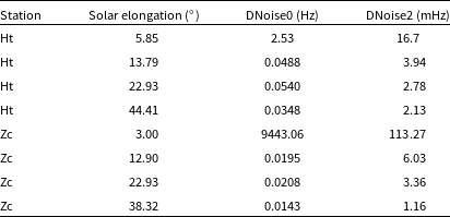
The RMS DNoise0 (Hz) and DNoise2 (mHz) values for Ht and Zc show a significant decrease with increasing solar elongation, indicating sensitivity to this parameter. The key values are summarised in Table 3. The variation in Doppler noise across different solar elongations is illustrated in Fig. 6, which presents results from the Ht sessions.
Doppler Noise values (DNoise0 in Hz, DNoise2 in mHz) for Ht and Zc at Different solar elongations.
A comparison of the Doppler noise levels (DNoise0-top, DNoise2-bottom) at different solar elongations. The sessions conducted at Ht were from 2015.07.05 (5.85 $^\circ$
), 2015.08.01 (13.79
$^\circ$
), 2015.08.01 (13.79 $^\circ$
), 2015.08.30(22.93
$^\circ$
), 2015.08.30(22.93 $^\circ$
) and 2015.10.13(44.41
$^\circ$
) and 2015.10.13(44.41 $^\circ$
).
$^\circ$
).
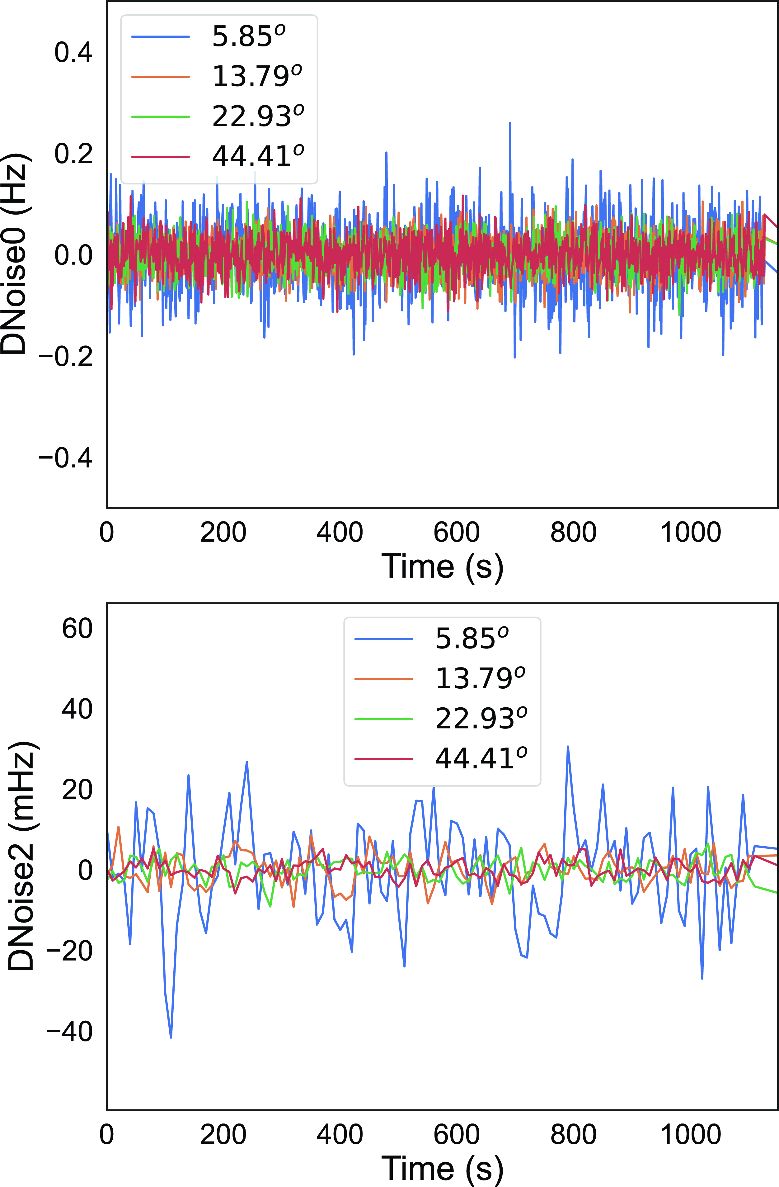
The ratios of DNoise0 to DNoise2 for each elongation provide additional insights. For Ht, the ratios range from 151.44 at 5.85 $^\circ$
to 16.34 at 44.41
$^\circ$
to 16.34 at 44.41 $^\circ$
. For Zc, the ratios start at an extremely high value of 83 366.51 at 3.00
$^\circ$
. For Zc, the ratios start at an extremely high value of 83 366.51 at 3.00 $^\circ$
before stabilizing at 3.23 at 12.90
$^\circ$
before stabilizing at 3.23 at 12.90 $^\circ$
, 6.18 at 22.93
$^\circ$
, 6.18 at 22.93 $^\circ$
, and 12.25 at 38.32
$^\circ$
, and 12.25 at 38.32 $^\circ$
. These findings reveal a significant difference between the ratios for elongations less than 10
$^\circ$
. These findings reveal a significant difference between the ratios for elongations less than 10 $^\circ$
and those at higher elongations, indicating a shift in the dominant noise sources. The drastic variation at lower elongations suggests the influence of coronal effects, while the stabilization at higher elongations points to more consistent noise levels.
$^\circ$
and those at higher elongations, indicating a shift in the dominant noise sources. The drastic variation at lower elongations suggests the influence of coronal effects, while the stabilization at higher elongations points to more consistent noise levels.
To investigate further, we focus on the narrowband DNoise2 values across multiple stations (Zc, Sh, Wd, Yg, Bd, Sv, Ho, and Wz), grouped into four solar elongation ranges: $\lt$
7
$\lt$
7 $^\circ$
, 10–20
$^\circ$
, 10–20 $^\circ$
, 20–30
$^\circ$
, 20–30 $^\circ$
, and
$^\circ$
, and $\gt$
30
$\gt$
30 $^\circ$
. In the
$^\circ$
. In the $\lt$
7
$\lt$
7 $^\circ$
range, DNoise2 is highest, with Zc reaching 71.82 mHz and most stations averaging 40–50 mHz. In the 10–20
$^\circ$
range, DNoise2 is highest, with Zc reaching 71.82 mHz and most stations averaging 40–50 mHz. In the 10–20 $^\circ$
range, the values drop significantly, ranging from 4.22 mHz (Wz) to 9.98 mHz (Bd). A further decrease is observed in the 20–30
$^\circ$
range, the values drop significantly, ranging from 4.22 mHz (Wz) to 9.98 mHz (Bd). A further decrease is observed in the 20–30 $^\circ$
range, with values between 2.89 mHz (Wd) and 9.25 mHz (Sv), indicating a more stable environment. At
$^\circ$
range, with values between 2.89 mHz (Wd) and 9.25 mHz (Sv), indicating a more stable environment. At $\gt$
30
$\gt$
30 $^\circ$
, DNoise2 is consistently the lowest, ranging from 1.55 mHz (Wz) to 3.46 mHz (Ho). This variation aligns with previous plasma studies (Molera Calvés et al. Reference Molera Calvés2014; Kummamuru et al. Reference Kummamuru2023), which show that phase residuals obtained from the digital Phase-Locked Loop (dPLL) are higher at lower solar elongations, closer to the Sun. These results confirm that narrowband Doppler noise is strongly influenced by solar elongation, with coronal effects being the dominant contributor at smaller elongation angles.
$^\circ$
, DNoise2 is consistently the lowest, ranging from 1.55 mHz (Wz) to 3.46 mHz (Ho). This variation aligns with previous plasma studies (Molera Calvés et al. Reference Molera Calvés2014; Kummamuru et al. Reference Kummamuru2023), which show that phase residuals obtained from the digital Phase-Locked Loop (dPLL) are higher at lower solar elongations, closer to the Sun. These results confirm that narrowband Doppler noise is strongly influenced by solar elongation, with coronal effects being the dominant contributor at smaller elongation angles.
4.3 Plasma propagation noise
Solar plasma is a major source of propagation error that is added to the Doppler data and forms an important part of formulating the overall noise budget. We look at how the frequency stability of the signal is affected at different solar offsets.
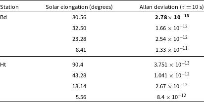
From the MEX campaign, sessions from Bd and Ht were chosen to understand how solar elongation affects the Allan deviation of plasma propagation noise. The two stations were selected because they observed over a wider range of solar elongations. These findings are crucial for understanding the limitations and capabilities of our tracking systems under varying solar conditions. The Allan deviation of the plasma propagation noise (Equation 6) for Badary and Hartbeesthoek is determined at different solar elongations, as seen in Table 4. When the signal propagation path nears the Sun’s corona, an increase in frequency dispersion is anticipated, primarily from increased solar activity and denser plasma medium. The effect of the solar corona diminishes beyond elongations of 15 degrees, which is reflected in the noise levels that drop by nearly 10 $\%$
. However, this remains consistent as the solar elongation increases from 18.14 to 43.28 degrees. Thus, confirming lesser propagation noise from solar plasma at higher elongations.
$\%$
. However, this remains consistent as the solar elongation increases from 18.14 to 43.28 degrees. Thus, confirming lesser propagation noise from solar plasma at higher elongations.
Allan deviation for the plasma scintillation noise at Badary (Bd) and Hartbeesthoek (Ht). The values are derived from individual station sessions meeting the specified solar elongation criteria.
4.4 Analysis of co-located stations
Co-located stations provide a unique opportunity to identify and isolate instrumental effects. By comparing observations from co-located antennas, we can evaluate the contributions of antenna design, physical factors, and signal processing within the overall noise budget. The co-located telescopes are expected to exhibit nearly identical propagation noise effects, as indicated by their similar scintillation indices derived from the low-frequency regions ( $\lt$
1 Hz) in the phase power spectrum (Fig. 1). We look to identify artifacts from individual telescope systems from these sessions and see if they can be isolated.
$\lt$
1 Hz) in the phase power spectrum (Fig. 1). We look to identify artifacts from individual telescope systems from these sessions and see if they can be isolated.
The co-located station pairs at Wettzell in Germany and Hobart in Australia are used for this study. To separate the phase noise contributions from different sources, we used concurrent sessions held at Wettzell (Wz & Wn) in 2015 and at Hobart (Ho & Hb) in 2023.
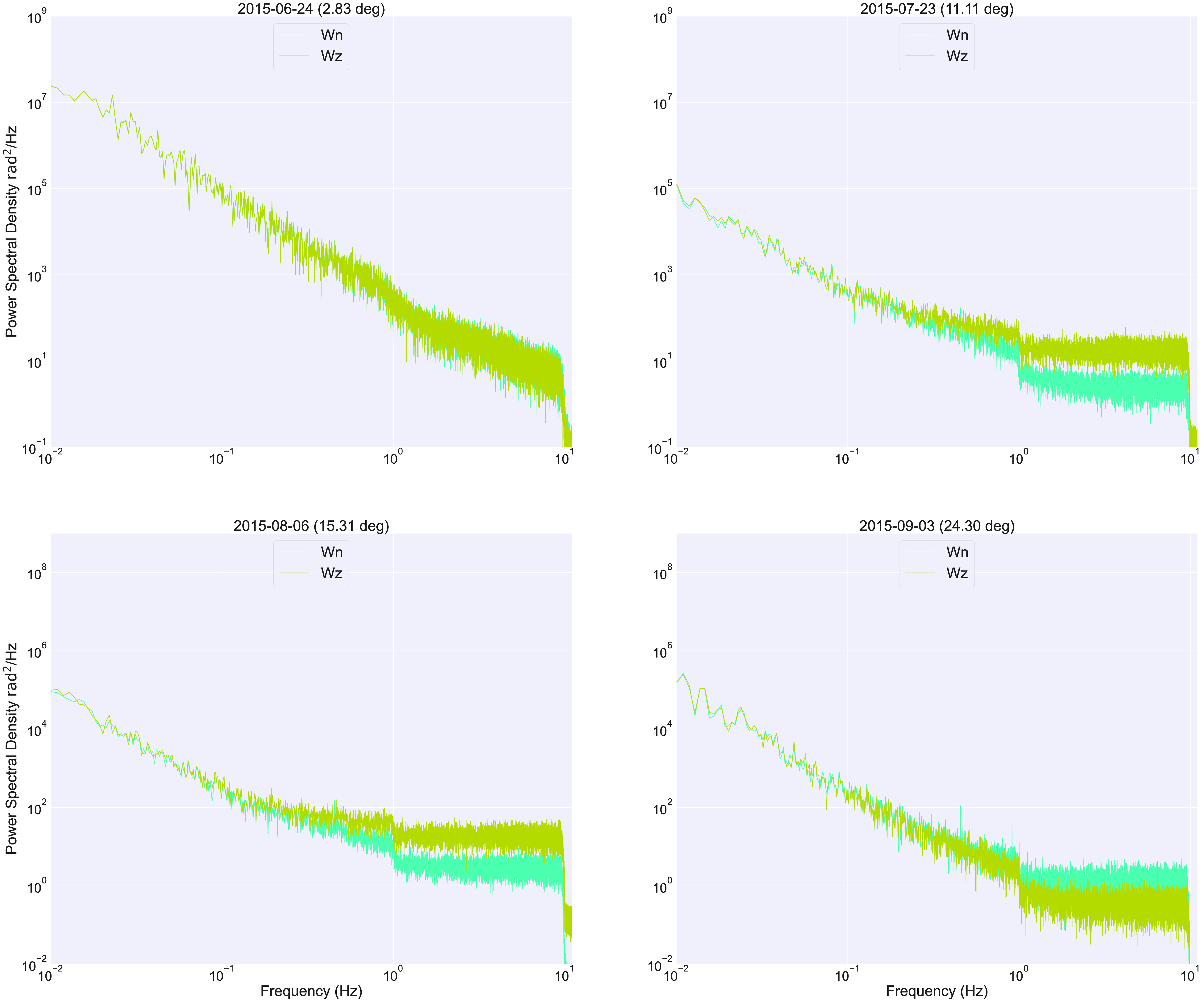
In 2015, four MEX observation sessions were held at Wettzell using the 20 m radio telescope (Wz) and one of the 13.2 m twin radio telescopes (Wn). The phase power spectra of selected sessions are given in Fig. 7. Sessions with smaller solar elongation exhibit an enhanced peak spectral density, leading to larger frequency instability introduced by plasma propagation noise. The session on 24 June 2015 showed a clear saturation of the system noise band at higher frequencies, attributable to the observational’s path proximity to the solar corona. However, in the following sessions, the system phase noise levels differ between both stations, indicating a signature of their individual instrument effects. The 24 June session was conducted during the solar conjunction, causing the system noise band to be saturated by plasma effects in the higher frequency regions. The system phase noise values are nearly the same for both these sessions. The 23 July and 06 August sessions, at solar elongations of 11.11 $^{\textbf{o}}$
and 15.31
$^{\textbf{o}}$
and 15.31 $^{\textbf{o}}$
show a difference in system phase noise of
$^{\textbf{o}}$
show a difference in system phase noise of $\sim0.03$
radians, with the 20 m Wz exhibiting greater phase error. For the session on 9 September (24.3 degrees), the noise band in the smaller Wn is found to be higher. The elevated system noise levels for Wz compared to Wn in the spectrum for the sessions on 23 July and 6 August suggest mechanical and thermal noise dominating in the larger telescope. The session on 9 September shows the smaller telescope having a higher system phase noise, likely due to the antenna’s backend. This suggests that system noise is not dominated by a single source.
$\sim0.03$
radians, with the 20 m Wz exhibiting greater phase error. For the session on 9 September (24.3 degrees), the noise band in the smaller Wn is found to be higher. The elevated system noise levels for Wz compared to Wn in the spectrum for the sessions on 23 July and 6 August suggest mechanical and thermal noise dominating in the larger telescope. The session on 9 September shows the smaller telescope having a higher system phase noise, likely due to the antenna’s backend. This suggests that system noise is not dominated by a single source.
The phase power spectra of the MEX sessions held between 24 June 2015 and 3 September 2015 at the co-located stations of Wettzell 13.2 m (Wn) and Wettzell 20 m (Wz). The solar elongations for the respective sessions are given in the brackets adjacent to the epoch.
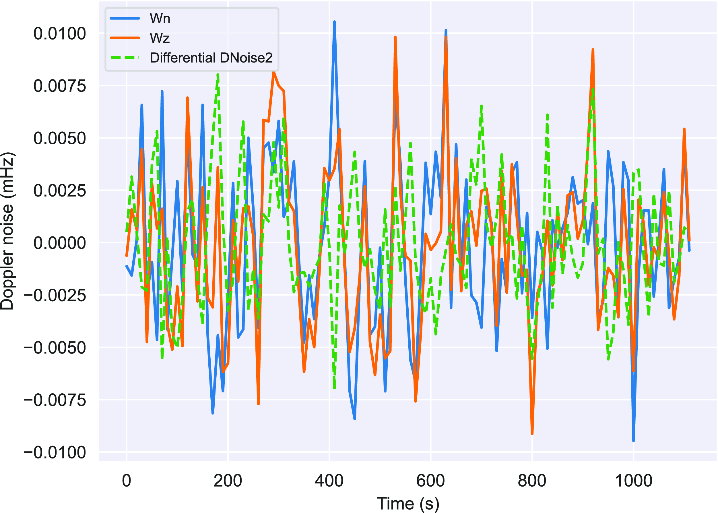
The individual stations’ Doppler noise (DNoise2) is visualised for these sessions to further support the previous results. As solar elongation increases, DNoise2 changes from strong to partially correlated. The correlation coefficient between the DNoise2 levels between Wz and Wn on the 24 June 2015, session is 0.968 mHz, indicating a strong ordinal relationship between the antennas (Fig. 8). This is likely a result of the session being close to solar conjunction (2.83 degrees elongation), which leads to a domination of the solar propagation noise on both antennas. In contrast, in the session on 06 August 2015 (Fig. 9), which is farther away from the Sun with a solar elongation of 15.31 degrees, the correlation coefficient is 0.65. This is where we start to see diminishing noise levels from solar plasma, and the individual instrumental noises dominate the Doppler noise. The RMS of the differential signal shows the difference in levels of the two Wettzell antennas’ noise as 0.003 mHz. This is in agreement with the results presented in Molera Calvés et al. (Reference Molera Calvés, Neidhardt, Plötz, Khronschnabl, Cimó and Pogrebenko2016).
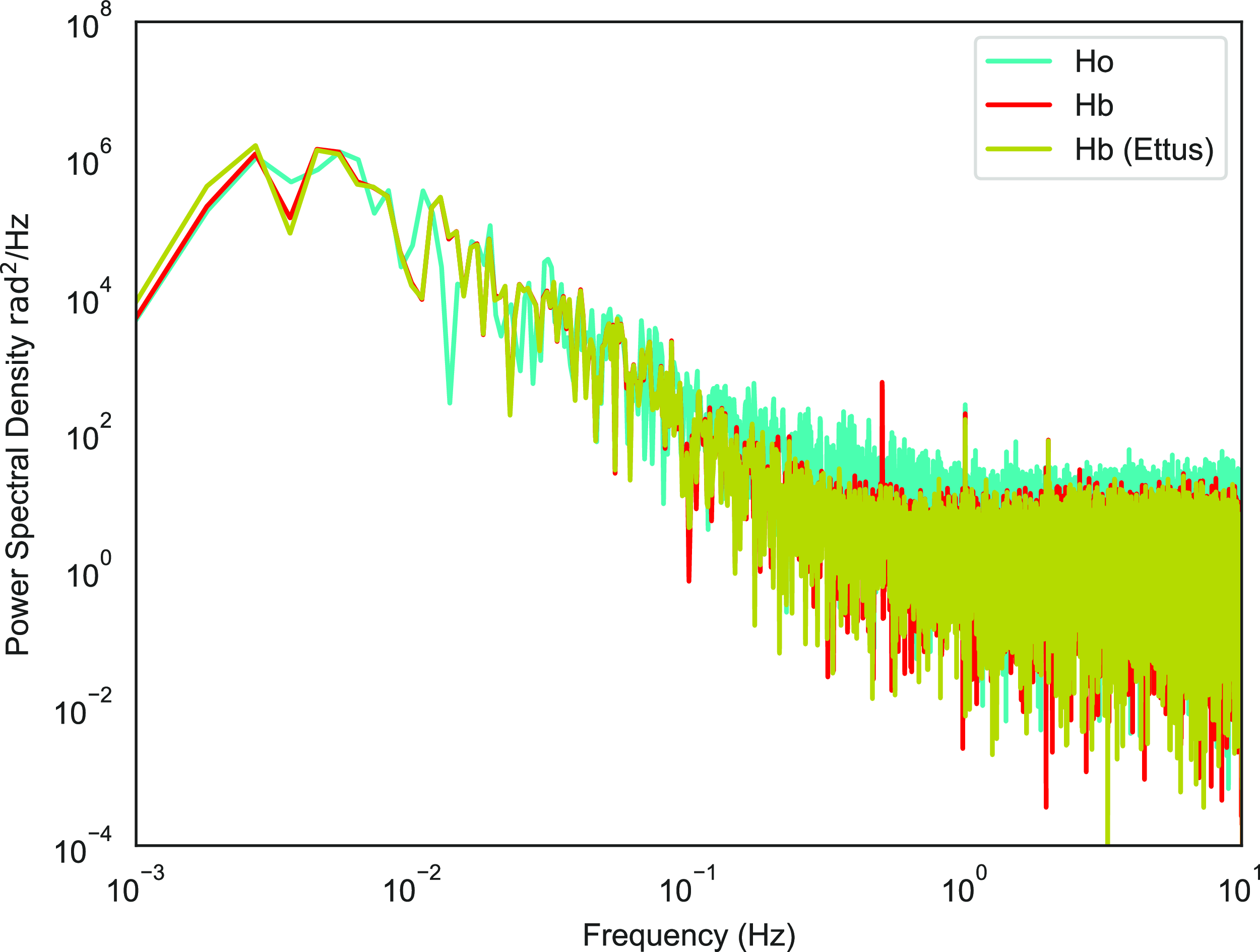
The use of co-located telescopes was replicated with Hb (12 m) and Ho (26m) in 2023. The session was recorded in both VDIF and in a different raw format using the ‘Ettus’ (Base 2020) which is an alternate software-defined radio device for sampling and digitization. Fig. 10 shows the power spectral densities of the Hb (VDIF), Ho (VDIF) and Hb (Ettus) plotted together from the session on 6 February 2023. The Ettus is a different backend that receives the signal from the Hb antenna with a spectrum that is similar to that of DBBC. The propagation effects visible in the lower frequency end are matched for all three systems. However, in the system noise band at higher frequencies (past 0.1 Hz), an elevated power is observed in Ho. The system phase noise of the Ettus device is comparable to that of the Hb receiver. This could indicate the domination of instrumental noises in the larger telescope.
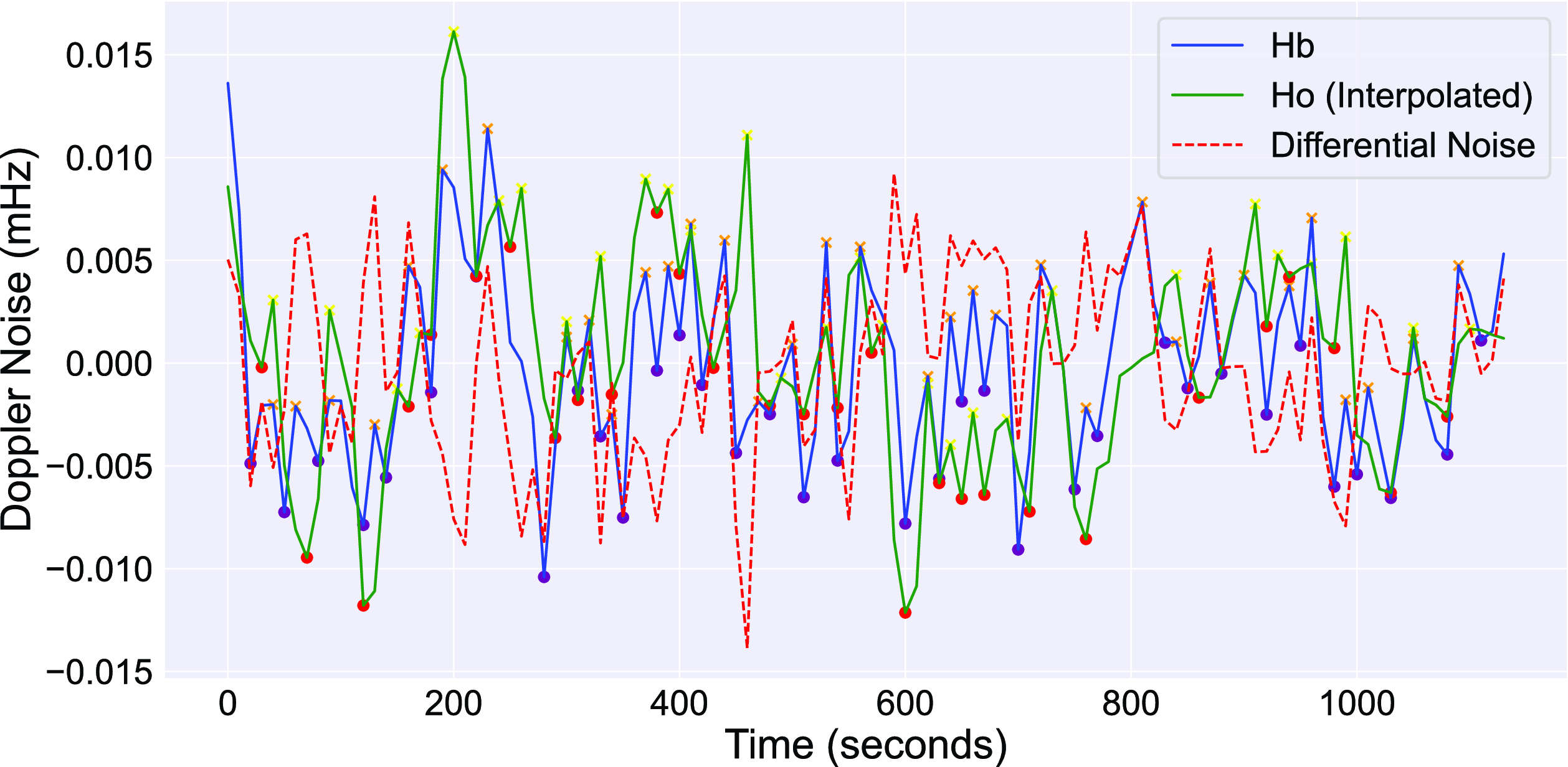
The Doppler noise fluctuations for Ho and Hb across two epochs are plotted in Figs. 11 and 12. The differential Doppler has a similar RMS value of approximately 0.004 mHz, which is in agreement with what we see with the Wettzell telescopes. The 11 May 2023, session shows distinct artifacts at the 400, 650, and 900 s for the Ho station. (Fig. 12). The power spectrum shows that both antennas have identical propagation effects, which suggests that these spikes in the Doppler noise are a feature native to the Ho instrumentation.
The Doppler noise (DNoise2) comparison between Wz and Wn from the session held on 24 June 2015. We see a strong correlation, which indicates the dominant effect of the solar plasma propagation noise compared to the other noise sources.
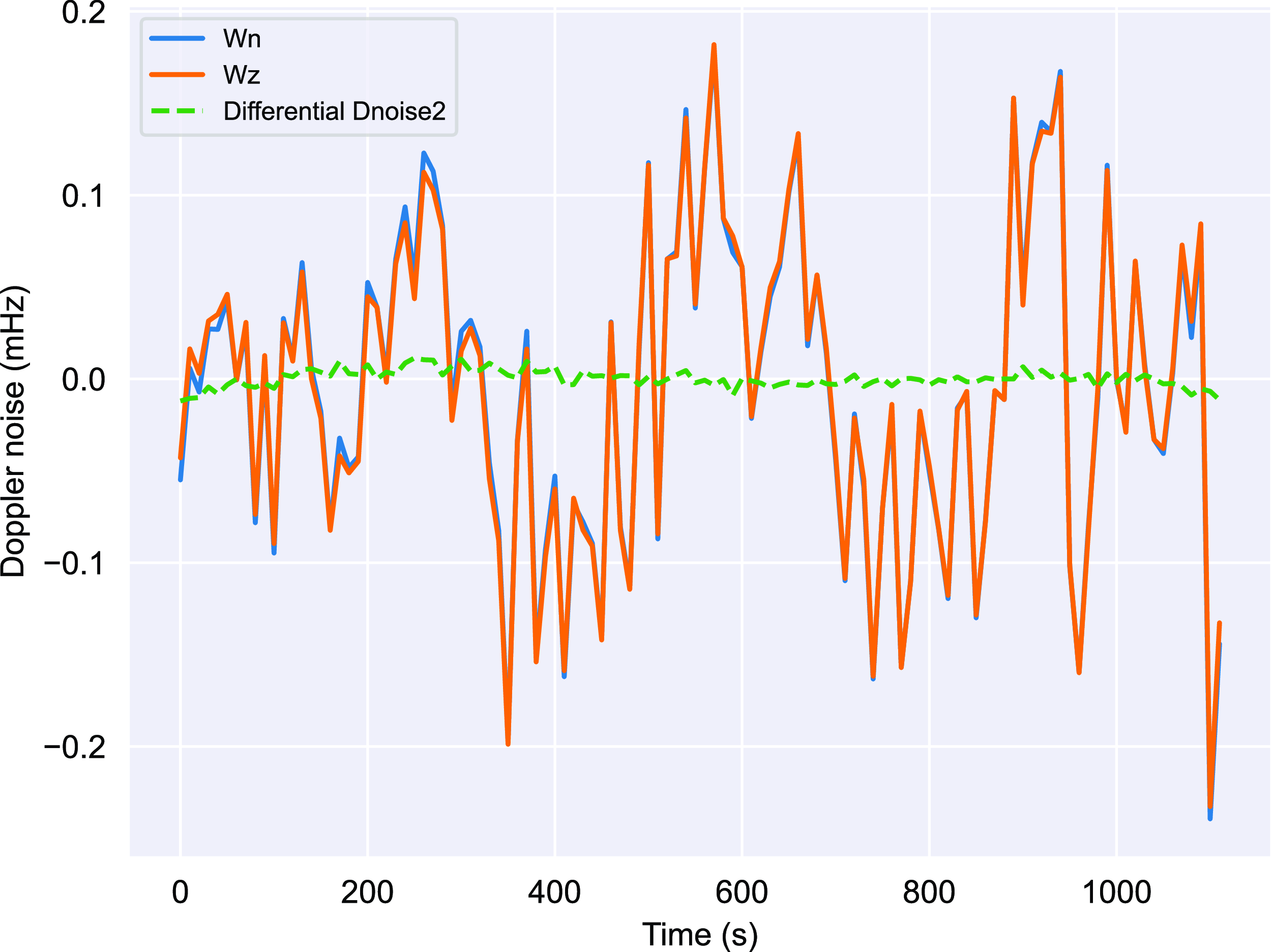
The Doppler noise (DNoise2) comparison between Wz and Wn from the session held on 6 August 2015. The spacecraft is further away from the Sun with a solar elongation of 15.31 degrees; hence, we start to see significant contributions from instrumental noises and not the solar plasma propagation dominating. Thus, we don’t see the same strong correlation as the previous session.
The power spectral density comparison of the co-located Hobart 12 and 26 m telescopes. Towards the higher end of frequencies where system noise dominates, a higher system phase noise level is observed at larger frequencies for Ho.
The Doppler noise fluctuation plot on 6 February 2023 for Hb and Ho with the peaks and troughs marked to highlight the resemblance in the pattern. The red dotted line is the differential noise between both stations.
The Doppler noise fluctuation plots from 11 May 2023, with peaks and troughs marked, show intrinsic features of the Ho system between 300 and 1 000 s, causing an elevated Doppler noise. This is distinctly visible in the differential noise plot.

The Doppler noise fluctuations of the spacecraft signal are more dependent on the propagation effects than the radio frequency and digital chain infrastructure. The Doppler noise is weighted to the SNR of the signal, which is dependent on the RMS of the noise level. The noise level is a feature intrinsic to the spectrum of the individual station. The RMS of the base noise level in Ho was $10^7$
dbM/Hz and for Hb was
$10^7$
dbM/Hz and for Hb was $10^8$
dbM/Hz which could be an explanation for the variations in the Doppler noise on the mHz level.
$10^8$
dbM/Hz which could be an explanation for the variations in the Doppler noise on the mHz level.
4.5 Phase calibration
Phase calibration (PCal) links the theoretical aspects of system performance and the practical challenges of achieving accurate phase correction. The PCal signal, typically a known and stable frequency tone, is injected into the signal path at the ground station and serves as a reference to calibrate phase noise and delay introduced by the receiver, cables, electronics, digitiser and recorder. We employed a phase calibration (PCal) procedure during the MEX observation campaign in 2014 and 2015 using telescopes at Hartebeesthoek (15 m), Wettzell (20 m), Hobart (12 m), and Yarragadee (12 m). The remaining stations either lacked a operational PCal system or were not enabled during observations. By injecting a stable frequency tone into the signal path, the PCal signal is processed identically to the spacecraft tone, allowing for the calibration of phase noise, phase scintillation, and system phase noise. This calibration process helps identify phase errors caused by Doppler shifts and signal delays, ensuring more accurate and reliable measurements.
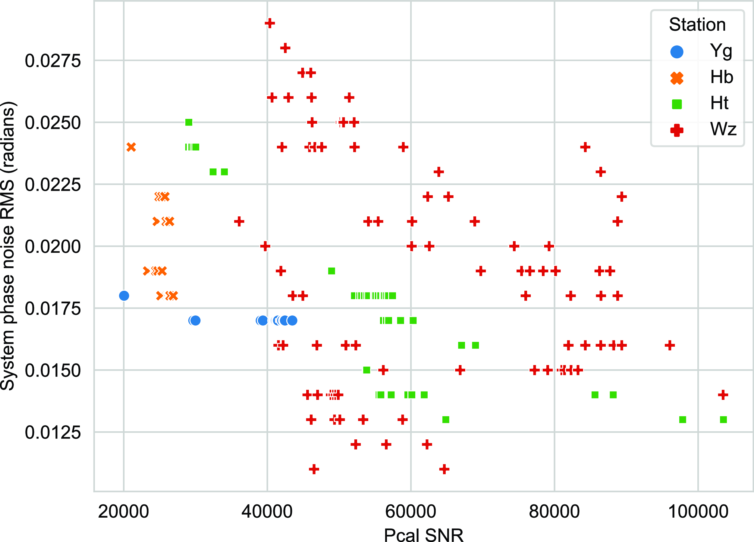
We quantified the system phase noise level in the higher frequency end of the post-PLL power spectrum for the PCal tone and see how it varies with the PCal SNR level obtained after dPLL. A lower SNR value can be indicative of a weaker narrowband signal or a higher noise baseband value. Fig. 13 shows a general consistency in showing that the system noise levels are higher for lower SNR values. This is consistent with what was seen in the earlier part of the section for the spacecraft signal.
The system phase noise RMS from the sessions that used the phase calibration comparison to the SNR values of the PCal tones.
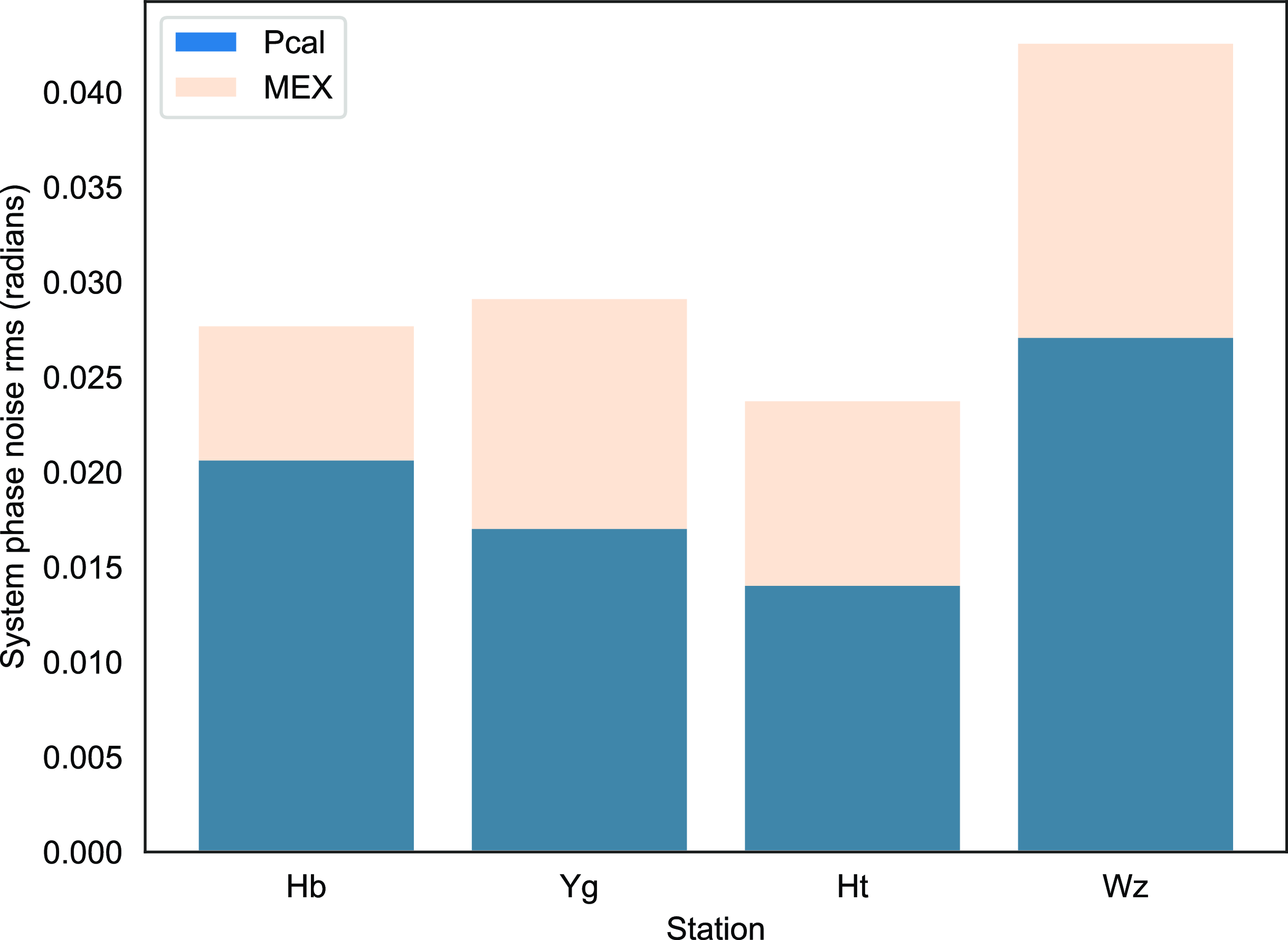
The system phase noise RMS obtained from the higher frequency band ( $\gt$
1 Hz) of the power spectrum is compared for the MEX signal and the PCal tone in Fig. 14. The PCal noise represents the effect of additional factors from the antenna system, atmosphere, and environment introduce phase errors into the MEX signal. The average level of phase noise introduced from these sources is about 0.011 radians and constitutes about 25–40% of the system phase noise level. Using the PCal as the system reference control, we can minimise these additional phase errors for each antenna. Thus improving the precision of orbit determination and navigation.
$\gt$
1 Hz) of the power spectrum is compared for the MEX signal and the PCal tone in Fig. 14. The PCal noise represents the effect of additional factors from the antenna system, atmosphere, and environment introduce phase errors into the MEX signal. The average level of phase noise introduced from these sources is about 0.011 radians and constitutes about 25–40% of the system phase noise level. Using the PCal as the system reference control, we can minimise these additional phase errors for each antenna. Thus improving the precision of orbit determination and navigation.
A comparison of the mean system noise of the MEX signal (ivory) and the injected phase calibration tone (blue) obtained from the post-PLL phase power spectrum. Note: The MEX noise bar plot (ivory) starts at 0 and is greater than the PCal noise.
5. Conclusions
Doppler spacecraft tracking is an important radiometric technique used for the scientific investigation of the Solar System and precise orbit determination of a spacecraft. Understanding the quantitative effect of different noise sources is critical to understand the method’s precision. This not only provides an understanding of these systems’ performance but also aids in improving the accuracy of radio science experiments and spacecraft astrometry. The MEX observation campaign between 2013 and 2020 (Kummamuru et al. Reference Kummamuru2023) was conducted using Doppler tracking with VLBI antennas, which provides an experimental platform to study and characterise the noise sources affecting the spacecraft carrier signal.
We determined the frequency stability of the thermal noise for each station; the Allan deviations value range between $7.071\times10^{-15}$
and
$7.071\times10^{-15}$
and $1.006\times10^{-13}$
, which are comparable to the open-loop Doppler data results presented by Bocanegra-Bahamón et al. (Reference Bocanegra-Bahamón, Molera Calvés, Gurvits, Duev, Pogrebenko, Cimò, Dirkx and Rosenblatt2018). The results show how the thermal stability varies across different antenna backends. The Allan deviation for the plasma propagation noise was calculated for the stations at Bd and Ht across solar elongations between
$1.006\times10^{-13}$
, which are comparable to the open-loop Doppler data results presented by Bocanegra-Bahamón et al. (Reference Bocanegra-Bahamón, Molera Calvés, Gurvits, Duev, Pogrebenko, Cimò, Dirkx and Rosenblatt2018). The results show how the thermal stability varies across different antenna backends. The Allan deviation for the plasma propagation noise was calculated for the stations at Bd and Ht across solar elongations between $5.56^{\text{o}}$
and
$5.56^{\text{o}}$
and $90.4^{\text{o}}$
with an Allan deviation around
$90.4^{\text{o}}$
with an Allan deviation around $10^{-13}$
. Increased instability closer to the conjunction was noticed, attributable to the strong effects of the solar corona near the Sun. The overall sensitivity is suitable for interplanetary plasma studies and orbit determination; however, to make the experiment sensitive to precise studies like general relativity measurements, would need to be rescued the noise of each principal component to
$10^{-13}$
. Increased instability closer to the conjunction was noticed, attributable to the strong effects of the solar corona near the Sun. The overall sensitivity is suitable for interplanetary plasma studies and orbit determination; however, to make the experiment sensitive to precise studies like general relativity measurements, would need to be rescued the noise of each principal component to $10^{-15}$
at 10 s (Iess et al. Reference Iess2003).
$10^{-15}$
at 10 s (Iess et al. Reference Iess2003).
The system phase noise levels from the post-PLL power spectrum were compared to the antenna’s sensitivities, which showed a generally proportional relationship with improvement in SNR, reducing the system phase noise to a certain degree. Thus, antennas with higher sensitivity are not as critical for plasma studies as they can be for radio occultation and planetary flyby experiments.
The Doppler noise analysis, examining variations with factors such as antenna size, solar elongation, and elevation angle yielded several important results. The impact of antenna size on wideband Doppler noise levels was evident, with the larger Sv (32 m) antenna outperforming the smaller Ht (15 m) and Mh (14 m) antennas (Fig. 4), achieving up to 15 times lower widebandd Doppler noise levels. In contrast, the difference is less pronounced in narrowband Doppler noise, where the dPLL’s precise narrowband processing refines frequency detections. The analysis of Doppler noise variation with elevation angle shows atmospheric effects dominating at lower angles (Fig. 5). The analysis was conducted for all sets of data that are individually affected by different path effects and intrinsic, instrumental noises that are expected to be dominant. While Doppler noise is generally higher at lower elevation angles, accurately isolating the atmospheric effects requires using advanced mapping functions and empirical models like the Vienna Mapping Function 3 and the Global Pressure and Temperture 3 (VMF3 and GPT3) (Landskron & Böhm Reference Landskron and Böhm2018). Solar elongation emerged as a factor influencing both wideband and narrowband Doppler noise. For the sessions at Ht and Zc, both Doppler noise levels decreased with increasing solar elongation, highlighting the sensitivity of Doppler noise to plasma effects, which dominate at lower elongations. The overall findings highlight the importance of optimizing observation parameters, such as antenna size, solar elongation, and elevation angle, to minimise Doppler noise.
Using co-located antennas allows for cross-examination of individual instrumental noise contributions because they experience identical path effects. The Wettzell and Hobart sessions from 2015 and 2023 showed differences in system phase noise levels. Fig. 7 shows that when the spacecraft is closer to solar conjunction, the entire range of frequencies in the power spectrum is dominated by the effects of the solar plasma. As the spacecraft moves farther from the Sun, the system noise band for the telescopes begins to vary, with smaller telescopes generally displaying higher levels of system phase noise. However, exceptions occur with the Wz (20 m) and Wn (13.2 m) telescopes. The Wz (20 m) telescope tends to exhibit greater system phase noise at higher solar elongations ( $\gt$
15 degrees) compared to Wn (13.2 m). This difference could possibly be attributed to the upgraded VGOS signal chain in Wn, in contrast to Wz’s legacy S/X band receiver. The VGOS system provides broadband capabilities over a wider frequency range and uses fiber optics instead of coaxial cables, ensuring higher stability and reduced signal loss (Petrachenko et al. Reference Petrachenko2015; Nilsson, Haas, & Varenius Reference Nilsson, Haas and Varenius2023). Another factor that could contribute to phase noise is the wind load, influenced by the aperture’s cross-sectional area, the surface drag coefficient, and wind pressure during the observation session.
$\gt$
15 degrees) compared to Wn (13.2 m). This difference could possibly be attributed to the upgraded VGOS signal chain in Wn, in contrast to Wz’s legacy S/X band receiver. The VGOS system provides broadband capabilities over a wider frequency range and uses fiber optics instead of coaxial cables, ensuring higher stability and reduced signal loss (Petrachenko et al. Reference Petrachenko2015; Nilsson, Haas, & Varenius Reference Nilsson, Haas and Varenius2023). Another factor that could contribute to phase noise is the wind load, influenced by the aperture’s cross-sectional area, the surface drag coefficient, and wind pressure during the observation session.
To examine specific telescope features, the Doppler noise levels were compared between stations, with Hobart and Wettzell exhibiting similar differential values of approximately 0.0035 mHz. This technique is valuable in distinguishing system noise artifacts from an elevated propagation feature (like a coronal mass ejection), as seen with the co-located Hobart telescopes from one of our observed sessions on 11 May 2023.
The introduction of the phase calibration tone during a part of the MEX campaign was useful to understand two things. The first was to confirm the generally lower system phase noise levels at higher SNR, as seen with the antennas. However, the margin is significantly lower than expected, given the known frequency stability of the PCal. The second part shows how the PCal can distinguish the inherent system noise from additional phase errors introduced by instrumental or atmospheric factors to the MEX signal. The average level of system phase noise introduced by non-backend sources is around 0.011 radians, comprising 25–40 $\%$
.
$\%$
.
Evaluating the quality of closed-loop Doppler data is important for planning future radio science experiments and spacecraft VLBI with recent missions like BepiColombo and JUICE using the PRIDE technique. To this end, we presented the noise budget for the long-term Doppler tracking of MEX while also detailing how different observational scenarios affect the output of Doppler data.
Acknowledgement
This study was possible thanks to the observations conducted by the different operators across EVN telescopes in China, Europe, Russia, Africa, and the AUT University (for Ww and Wa). The long-term study of plasma was also consolidated by the array of the Auscope VLBI telescopes operated by the University of Tasmania. The author acknowledges the valuable input from collaborators at Delft University, JIVE, the Chinese Natural Science Foundation and Key Incubation Project of Shanghai Astronomical Observatory. The data collection for research was possible thanks to the ESA’s MEX communication team. Note: From 1 July 2023, the operation of Warkworth was transferred from Auckland University of Technology (AUT) to Space Operations New Zealand Ltd.
Data availability
Data supporting the findings of this study are available from the corresponding author upon reasonable request.


 Open access