
Contents


1N.1 Overview
We will start by looking at circuits made up entirely of
DC voltage sources (things whose output voltage is constant over time; things like a battery, or a lab power supply); and …
resistors.
Sounds simple, and it is. We will try to point out quick ways to handle these familiar circuit elements. We will concentrate on one circuit fragment, the voltage divider.
1N.1.1 Why?
In each day’s class notes we will sketch the sort of task that the day’s material might let us accomplish. We do this to try to head off a challenge likely to occur to any skeptical reader: OK, this is a something-or-other circuit, but what’s it for? Why do I need a something-or-other? This is an integrator – but why do I want an integrator? Here is our first try at providing such a sample application:
Problem
Given a constant (“DC”) voltage source, design a lower voltage source, strong enough to “drive” a particular “load” resistance.
Shorthand version of the problem:
Make a voltage divider to deliver a specified voltage. Arrange things so that increasing load current to a maximum causes  to vary by no more than a specified percentage.
1N.1.2 What is “the art of electronics?”
Not art that you’re likely to find in a museum,Footnote 1 but art in an older sense: a craft.Footnote 2 No doubt the title of The Art of Electronics (hereafter referred to as “AoE”) was chosen with an awareness of the suggestion that there’s something borderline-magical available here: perhaps a hint of “black art”?
AoE §1.1
Here is AoE’s formulation of the subject of this course:
the laws, rules of thumb, sand tricks that constitute the art of electronics as we see it.
As you may have gathered, if you have looked at the text, this course differs from an engineering electronics course in concentrating on the “rules of thumb” and the bag of “tricks.” You will learn to use rules of thumb and reliable “tricks” without apology. With their help you will be able to leave the calculator-bound novice engineer in the dust!
1N.1.3 What the course is not about
Wire my basement? Fix my TV?
Alumni of this course sometimes are asked for help that is beyond their capacities, and sometimes below – or beside – what they know. “So, now you can wire some outlets in my basement?” No. This course won’t help much with that task, which is easy in a sense but difficult in another, in that it requires a detailed knowledge of electrical codes (required wire gauges; types of jacketing; where ground-fault-interrupters are required). And when your friend’s TV quits, you’re probably not going to want to fix it: much of the set’s circuitry will be embodied in mysterious proprietary integrated circuits; an effective repair – if it were economically worthwhile – would likely amount to ordering a replacement for a substantial module, rather than replacing a burned-out resistor or transistor, as in the good old days of big and fixable devices.
Delivering power
A subtler point is worth making as well: only now and then, in this course, do we undertake to deliver power to something (the “something” is conventionally called a “load”). Occasionally, we are interested in doing that: when we want to make a loud sound from a speaker, or want to spin a motor. But much more often, we would like to minimize the flow of power; we are concerned, instead, with the flow of information.
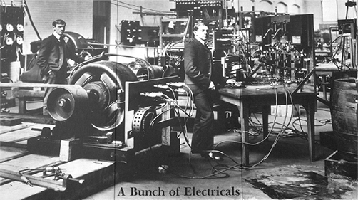
On the wall of the lobby of MIT’s Electrical Engineering building is a huge blowup of a photo of some MIT engineers standing among what look like large generators or motors, each about the size of a small cow. The photo in Fig. 1N.1 seems to date from the 1930s.

Figure 1N.1 Electronics ca. 1935 [used with permission of MIT.]
The “Electricals,” back then, were concerned mostly with those big machines: with delivering power. It was the power companies that were hiring, when one of our uncles finished at MIT, around 1936. Hoover Dam, finished in 1935, was the engineering wonder of the day. Big was beautiful. (Even now, Hoover Dam’s website boasts of the dam’s weight! – 6.6 million tons, in case you were wondering.)
1N.1.4 What the course is about: processing information
Times have changed, as you may have noticed. Small is beautiful; nano is extra beautiful – and electronics, these days, is concerned mostly with processing information.Footnote 3 So, we like circuits that pass and process signals while generating very little heat – using very little power. We like, for example, digital circuits made out of field-effect transistors that form switches; they offer low output impedance, gargantuan input impedance, and quiescent current of approximately zero. To a good approximation, they’re not transferring power, not using it, not delivering it. They’re dealing in information. That’s almost always what we’ll be doing in this course.
Obvious, perhaps? Perhaps.
We will postpone till next time – not to overload you, on the first day – discussion of a related topic: just what form the information is likely to take, in our circuits: voltage versus current. The answer may surprise you; or you may be inclined to reject the question as empty, since you know that long ago Ohm taught us that current and voltage in a device can be intimately related. Next time, we’ll try to persuade you that you ought not to reject the question; that it’s worth considering whether the signal is represented as a voltage or as a current (and see Note 1S on this topic).
Now on to less abstract topics, and our first useful circuit: a voltage divider.
1N.2 Three laws
AoE §1.2.1
A glance at three laws: Ohm’s law, and Kirchhoff’s laws (Voltage – “KVL,” and current – “KCL”).
We rely on these rules continually, in electronics. Nevertheless, we rarely will mention Kirchhoff again. We use his observations implicitly. By contrast, we will see and use Ohm’s law a lot; no one has gotten around to doing what’s demanded by the bumper sticker one sees around MIT: Repeal Ohm’s Law!
1N.2.1 Ohm’s law: V = IR
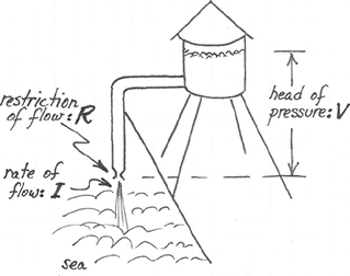
V is the analog of water pressure or ‘head’ of water.
R describes the restriction of flow.

Figure 1N.2 Hydraulic analogy: voltage as head of water, etc. Use it if it helps your intuition.
The homely hydraulic analogy works pretty well, if you don’t push it too far – and if you’re not too proud to use such an aid to intuition.
What is “voltage,” and other deeper questions
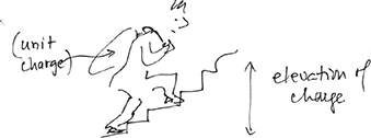
For the most part, we will evade such deep questions in this course. We’re inclined to say, “Oh, a Volt is what pushes an Amp through an Ohm.” But you don’t have to be quite so glib (you don’t have to sound so much like a Harvard student!). A less circular definition of voltage is the potential energy per unit charge. Or, equivalently, it can be defined as the work done to move a unit charge against an electric field (a word that we hope doesn’t worry you; we suggest you try to get accustomed to use of the word, even if you have reservations about its usefulnessFootnote 4), from one electric potential (analogous to a position on a hillside) to a higher potential (higher on the hillside).
The voltage difference between two points on the hillside (or staircase, as in Fig. 1N.3) can be described as a difference in electric potential or voltage. The so-called “electric field” will tend to push that charge back down, just as gravity will tend to pull the water down from the tank. You may or may not be interested to know that one volt is the work done as one adds one joule of potential energy to one coulomb of charge.Footnote 5 But we’ll not again speak in these terms – which sound more like physics than like language for the “art of electronics.”

Figure 1N.3 Voltage is work to raise a unit charge from one level to a higher level (or “potential”).
“Ground”
Sometimes we speak of a voltage relative to some absolute reference – perhaps the planet Earth (or, a bit more practically, the potential at the place where a copper spike has been driven into the ground, in the basement of the building where you are doing your electronics). In the hydraulic analogy, that absolute zero-reference might be sea-level. More often, as we will reiterate below, we are interested only in relative voltages: differences in potential, measured relative to an arbitrary reference point, not relative to planet Earth.
Ohm’s is a very useful rule; but it applies only to things that behave like resistors. What are these? They are things that obey Ohm’s Law! (Sorry folks: that’s as deeply as we’ll look at this question, in this course.Footnote 6)
Why does Ohm’s law hold?
The restriction of current flow that we call “resistance” – which we might contrast with the very-easy flow of current in a piece of wireFootnote 7 – occurs because the charge-carrying electrons, accelerated by an electric field, bump into obstacles (vibrations of the atomic lattice) after a short free flight, and then have to be re-accelerated in the direction of the field. Materials that are good conductors – metals – have a substantial population of electrons that are not tightly bound, and consequently are free to travel when pushed. The conductivity of a metal depends on the density of the population of charge carriers (usually, un-bound electrons), and it’s kind of reassuring to find that conductivity usually degrades with rising temperature: the free flights become shorter, as electrons bump into the jumpier atoms of the hotter material. This effect you will see confirmed in Lab 1L if things come out right in your experiment (you’ll have to do a little reasoning to see this effect confirmed; the notes to Lab 1L do not point out where this occurs). The stronger the field, the faster the drift of the electrons. Field strength goes with voltage difference between two points on the conductor; rate of drift of the electrons measures current. So, Ohm’s Law is pretty plausible.
What determines the value of a resistor?
AoE §C.4
A “resistor” is also, of course, a “conductor”; it may seem a bit perverse to call this thing that is inserted in a circuit to permit current flow a “resistor.” But the name comes from the assumption that the resistor is inserted where an excellent conductor – a piece of wire – might have stood, instead. To make a resistor, one can use either of two strategies: to make a “carbon composition” resistor (the sort that we’ll use in lab because their values are relatively easy to read), one mixes up a batch of powdered insulator and powdered conductor (carbon), adjusting the proportions to give the material a particular resistivity. To make a “metal film” resistor (much the more common type, these days), one “deposits” a thin film of metal on a ceramic substrate, and then partially cuts away the thin conducting film.
How generally does Ohm’s law apply?
We begin almost at once to meet devices that do not obey Ohm’s Law (see Lab 1L: a lamp; a diode). Ohm’s Law describes one possible relation between V and I in a component; but there are others. As AoE says,
Crudely speaking, the name of the game is to make and use gadgets that have interesting and useful I versus V characteristics.
In a resistor, current and voltage are proportional in a nice, linear way: double the voltage and you get double the current. Ohm’s Law holds. Don’t expect to use it where it doesn’t fit. Even the lamp – whose filament is just a piece of metal that one might expect would behave like a resistor – doesn’t follow Ohm’s Law, as you’ll see in Lab 1L. Why not?Footnote 8
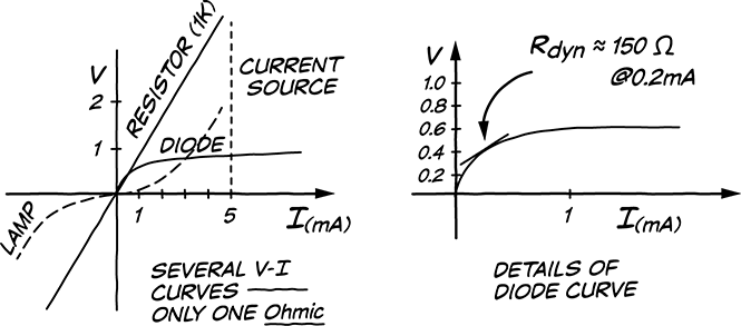
… But we can extend the reach of Ohm’s law? Dynamic resistance:
After today, we rarely will limit ourselves to devices that show simply resistance – and as we have said, even the resistor-like lamp that you meet in Lab 1L, along with the diode, defy Ohm’s-Law treatment. But an extended version of Ohm’s Law that we’ll call dynamic resistance will allow us to apply the familiar rule in settings where otherwise it would not work. The idea is just to define a local resistance – the tangent to the slope of the device’s V– I curve:

This redefinition allows us to talk about the effective resistance of a diode, a transistor, or a current source (a circuit that holds current constant). Here is a sketch of a diode’s V– I curve – oriented so that V is the vertical axis. This orientation puts the curves’ slopes into the familiar units, Ohms (rather than into  ,Footnote 9 as in the more standard I– V plot).
AoE §1.2.6

Figure 1N.4 Dynamic resistance illustrated: local slope can be defined for devices that are not Ohmic.
You may like the resistor’s well-behaved straight line, because it is familiar. But the nice thing about the notion of  is that is so broad-minded: it is happy to describe the V– I curve (or “ I– V curve,” as it is more often called) for any device. It will happily fit a transistor, an exotic current source, or just about anything. The nearly-vertical plot of the current source, implying enormous
  , will become important to your understanding of transistors.
Power in a resistor:
AoE §1.2.2C
Power is the rate of doing work, as you may recall from a course on mechanics. The concept comes up most often, in electronics, when one tries to specify a component that can safely handle the power that it is likely to have to dissipate. High power produces high heat, and calls for a component capable of unloading or dissipating that heat. The three resistors shown below illustrate the rough relation between power rating and size – because large size usually offers large area in contact with the surroundings or “ambient.”
The indicated power ratings show the maximum that each can dissipate without damage. The tiny “surface-mount” on the left (“’0805 size,” large by surface-mount standards) dissipates more than one might expect if one compares its size to that the of the 1/4 W carbon-comp (the sort we use in the lab); it does better than one might expect because it is soldered directly to a circuit board, whose copper traces help to draw off and dissipate its heat.
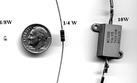
Figure 1N.5 Three resistors (plus a pretty good copper–nickel alloy conductor).
In the coming labs you will sometimes run into the question whether your components can handle the power that is expected. Our usual resistors are rated at 1/4 W. You can confirm that such a resistor can handle 15 V (our usual maximum supply voltage) if the resistor’s value is at least  . Let’s try that calculation:
  .
.
Thanks to Ohm’s Law, the formula for power can be written in any of three ways:
 (as we just said); but since and
- ; and since ,
- .


In the present case, it is the last form that is most useful: 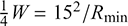 . So
. So  . So 1k is close to the minimum safe value, at 15 V (910 would be safe, but let’s not be so fussy; call it 1k).
So far, we have mentioned only power in a resistor. The notion is more general than that, and the formula

holds for any electronic component.
A closer look at what we mean by V and I makes this formula seem almost obvious:
current measures charge/time; and
voltage measures work/charge.
So, the product,  = work/charge × charge/time = work/time, and this is power.
In this course, the exceptional cases where we do worry about power are those cases in which we either use large voltage swings (for example, the 30 V output swing of the “comparator” in Lab 8L) or want to provide unusually large currents (for example, the speaker drive of Lab 6L, the light-emitting diode drive of the music-transmission lab, 13L, and the voltage regulators of Lab 11L).
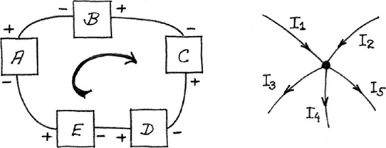
1N.2.2 Kirchhoff’s laws: V, I
These two ‘laws’ probably only codify what you think you know through common sense:
Sum of voltages around the loop (or “circuit”) is zero; see Fig. 1N.6, left.
Sum of currents in and out of a node is zero (algebraic sum, of course); see Fig. 1N.6, right.

Figure 1N.6 Kirchhoff’s two laws. Left: KVL – sum of voltages around a loop is zero; right: KCL – sum of currents in and out of a node is zero.
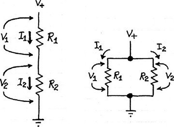
Figure 1N.7 Applications of Kirchhoff’s laws: series and parallel circuits: a couple of truisms, probably familiar to you already.
Applications of these laws: series and parallel circuits:
| Series |  |  |
| Parallel |  |  |
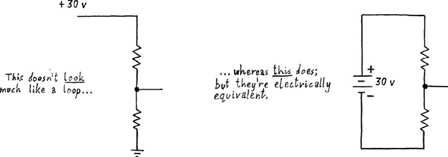
Query Incidentally, where is the “loop” that Kirchhoff’s law refers to? Answer: the “loop” (or “circuit,” a near-synonym) is apparent if one draws the voltage source as a circuit element, and ties its foot to the foot of the R: see Fig. 1N.8.

Figure 1N.8 Voltage divider redrawn to look more like a “loop” or “circuit”.
Usually we don’t bother to draw the voltage source that way; we label points with voltage values, and assume that you can picture the circuit path for yourself, if you choose to.
This is kind of boring. So, let’s hurry on to less abstract circuits: to applications – and tricks. First, some labor-saving tricks.
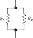
Parallel resistances: calculating equivalent R
The conductances add:


Figure 1N.9 Parallel resistors: the conductances add; unfortunately, the resistances don’t.
This is the easy notion to remember, but not usually convenient to apply, for one rarely speaks of conductances. The notion “resistance” is so generally used that you will sometimes want to use the formula for the effective resistance of two parallel resistors:

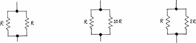
Believe it or not, even this formula is messier than what we like to ask you to work with in this course. So we proceed immediately to some tricks that let you do most work in your head. Consider the easy cases in Fig. 1N.10. The first two are especially important, because they help one to estimate the effect of a circuit one can liken to either case. Labor-saving tricks that give you an estimate are not to be scorned: if you see an easy way to an estimate, you’re likely to make the estimate. If you have to work too hard to get the answer, you may find yourself simply not making the estimate. A deadly trap for the student doing a lab is the thought, “Oh, I’ll calculate this later – some time this evening, when I’m comfortable in front of a spreadsheet.” This student won’t get to that calculation! The leftmost case in Fig. 1N.10 surely doesn’t call for pulling out a formula: two equal Rs paralleled behave like  . The middle case is easier still, given that we’re willing to ignore errors under 10%. (On the other hand, when you do want to trim an R value by 10% this is an easy way to do just that.) The rightmost calls for slightly more imagination: think of the lone R as a paralleling of two resistors of equal value:
  . Then the whole looks like three paralleled resistors, each of value 2R. The result then is
  .
.

Figure 1N.10 Parallel Rs: Some easy cases.
AoE §1.2.2B
In this course we usually are content with answers good to 10%. So, if two parallel resistors differ by a factor of ten or more, then we can ignore the larger of the two.
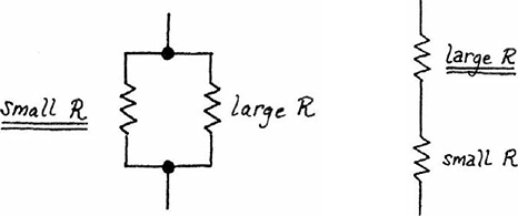
Let’s elevate this observation to a rule of thumb (our first). While we’re at it, we can state the equivalent rule for resistors in series.

Figure 1N.11 Resistor calculation shortcut: parallel, series. In a parallel circuit, a resistor much smaller than others dominates. In a series circuit, the larger resistor dominates.
1N.3 First application: voltage divider
AoE §1.2.3
Why dividers?
Are dividers necessary? Why not start with the right voltage? The answer, as you know, is just that a typical circuit needs several voltages, and building a “power supply” to deliver each voltage is impractical (meaning, mostly, expensive). You’ll soon be designing power supplies, and certainly at that time will appreciate how much simpler a voltage divider is, compared to a full power supply.
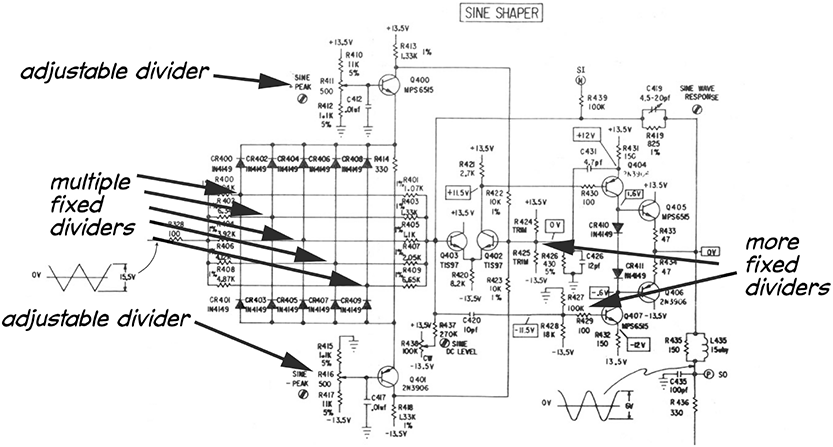
To illustrate the point that voltage dividers are useful, and not just an academic device used to provide an easy introduction to circuitry, we offer here a piece of a fairly complex device, a “function generator” – the box that soon will be providing waveforms to the circuits that you build in Lab 2L. Figure 1N.12 shows part of the circuitry that converts a triangular waveform into a sinusoidal shape.

Figure 1N.12 Voltage dividers in a function generator: dividers are not just for beginners [Krohn–Hite 1600 A function generator].
Aside: variable dividers or “potentiometers”:
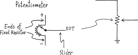
Before we look closely at an ordinary divider, let’s note a variation that’s often useful: a voltage divider that is adjustable. This circuit, available as a ready-made component, is called a “potentiometer.”

Figure 1N.13 Symbol for potentiometer, and its construction.
The name describes the circuit pretty well: the device “meters” or measures out “potential.” Recalling this may help you to keep separate the two ways to use the device:
as a potentiometer versus…, and
as a variable resistor.
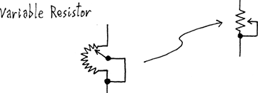
“Variable resistor:” just one way to use a pot:
The component is called a potentiometer (a 3-terminal device), but it can be used as a variable resistor (a 2-terminal device).

Figure 1N.14 A “pot” can be wired to operate as a variable resistor.
The pot becomes a variable resistor if one uses just one end of the fixed resistor and the slider, or if (somewhat better) one ties the slider to one end.Footnote 10
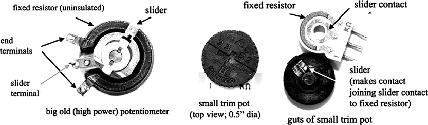
How the potentiometer is constructed:
It helps to see how the thing is constructed. In Fig. 1N.15 are photos of two potentiometers. It is not hard to recognize how the large one on the left works. A (fixed) wire-wound resistor, not insulated, follows most of the way around a circle. A sliding contact presses against this wire-wound resistor. It can be rotated to either extreme.

Figure 1N.15 Potentiometer construction details.
At the position shown, the contact seems to be about 70% of the way between lower and upper terminals. If the upper terminal were at 10 V and the lower one at ground, the output at the slider terminal would be about 7 V.
The smaller pot shown in middle and right of Fig. 1N.15 (and shown enlarged, relative to the left-hand device) is fundamentally the same, but constructed in a way that makes it compact. Its fixed resistor – of value  – is made not of wound wire but of “cermet.”Footnote 11
1N.3.1 A voltage divider to analyze
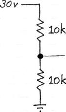
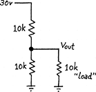
Figure 1N.16 is a simple example of the more common fixed voltage divider. At last we have reached a circuit that does something useful. It delivers a voltage of the designer’s choice; a voltage less than the original or “source” voltage.

Figure 1N.16 Voltage divider.
First, a note on labeling: we label the resistors “10k”; we omit “ .” It goes without saying. The “k” means kilo- or
  , as you probably know.
One can calculate  in several ways. We will try to push you toward the way that makes it easy to get an answer in your head.
Three ways to analyze this circuit
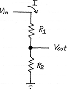
First method: calculate the current through the series resistance…:
Calculate the current (see Fig. 1N.17):

Figure 1N.17 Voltage divider: first method (too hard!): calculate current explicitly.

That’s  . After calculating that current, use it to calculate the voltage in the lower leg of the divider:

Here that product is  . That takes too long.
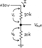
Second method: rely on the fact that I is the same in top and bottom…:
But rely on this equality only implicitly.

Figure 1N.18 Voltage divider: second method: (a little better): current implicit.
If you want an algebraic argument, you might say,

or,
 (1N.1)
In this case that means

That’s much better, and you will use formula (1N.1) fairly often. But we would like to push you not to memorize that equation, but instead to work less formally.
Third method: say to yourself in words how the divider works…:
Something like
Since the currents in top and bottom are equal, the voltage drops are proportional to the resistances (later, impedances – a more general notion that covers devices other than resistors).
So in this case, where the lower R makes up half the total resistance, it also will show half the total voltage.
For another example, if the lower leg is 10 times the upper leg, it will show about 90% of the input voltage (10/11, if you’re fussy, but 90%, to our usual tolerances).
1N.4 Loading, and “output impedance”
Now – after you’ve calculated  for the divider – suppose someone comes along and puts in a third resistor, as in Fig. 1N.19. (Query: Are you entitled to be outraged? Is this not fair?Footnote 12)

Figure 1N.19 Voltage divider loaded.
Again there is more than one way to make the new calculation – but one way is tidier than the other.
1N.4.1 Two possible methods
Tedious method:
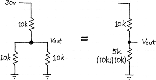
Model the two lower Rs as one R; calculate  for this new voltage divider: see Fig. 1N.20. The new divider delivers 1/3
  . That’s reasonable, but it requires you to draw a new model to describe each possible loading.

Figure 1N.20 Voltage divider loaded: load and lower R combined in model.
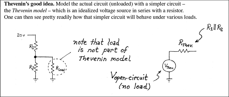
Better method: Thevenin’s model:
AoE §1.2.5
Here’s how to calculate the two elements of the Thevenin model:
Just
: the voltage out when nothing is attached (“no load”).Often formulated as the quotient of
, which is the current that flows from the circuit output to ground if you simply short the output to ground.


Figure 1N.21 Thevenin model: perfect voltage source in series with output resistance.
In practice, you are not likely to discover  by so brutal an experiment. Often, shorting the output to ground is a very bad idea: bad for the circuit and sometimes dangerous to you. Imagine the result, for example, if you decided to try this with a 12 V car battery! And if you have a diagram of the circuit to look at, a much faster shortcut is available: see Fig. 1N.22.

Figure 1N.22  parallel
  .
.
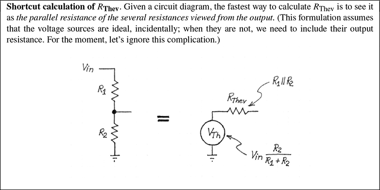
Shortcut calculation of  . Given a circuit diagram, the fastest way to calculate
  is to see it as the parallel resistance of the several resistances viewed from the output. (This formulation assumes that the voltage sources are ideal, incidentally; when they are not, we need to include their output resistance. For the moment, let’s ignore this complication.)
1N.4.2 Justifying the Thevenin shortcut
Our shortcut, shown in Fig. 1N.22, asserts that  , but the result still may strike you as a little odd: why should
  , going up to the positive supply, be treated as parallel to
  ? Well, suppose the positive supply were set at zero volts. Then surely the two resistances would be in parallel, right?
And try another thought experiment: redefine the positive supply as 0 V. It follows then that the voltage we had been calling “ground” or “zero volts” now is  V (to use the numbers of Fig. 1N.16). Now it seems clear that the upper resistor, to ground, matters; the lower resistor,
  , going to
  V now is the one that seems odd. But, of course, the circuit doesn’t know or care how we humans have chosen to define our “zero volts” or “ground.”
The point of this playing with “ground” definitions is just that the voltages at the far end of those resistors “seen” from the output do not matter. It matters only that those voltages are fixed.Footnote 13
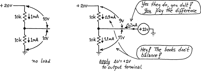
Or suppose a different divider (chosen to make the numbers easy): 20 V divided by two 10k resistors. To discover the impedance at the output, do the usual experiment (one that we will speak of again and again):
A general definition and procedure for determining impedance at a point:
| To discover the impedance at a point: |
apply a  ; find ; find  . . |
| The quotient is the impedance. |
You will recognize the circuits in Fig. 1N.23 as just a “small signal” or “dynamic” version of Ohm’s Law. In this case 1 mA was flowing before the wiggle. After we force the output up by 1 V, the currents in top and bottom resistors no longer match: upstairs: 0.9 mA; downstairs, 1.1 mA. The difference must come from you, the wiggler.

Figure 1N.23 Hypothetical divider: current = 1 mA; apply a wiggle of voltage,  V; see what
  I results.

And – happily – that is the parallel resistance of the two R s. Does that argument make the result easier to accept?
You may be wondering why this model is useful. Fig. 1N.23 shows one way to put the answer, though probably you will remain skeptical until you have seen the model at work in several examples.
AoE §1.2.6
Rationalizing Thevenin’s result: parallel Rs
Any non-ideal voltage source “droops” when loaded. How much it droops depends on its “output impedance.” The Thevenin equivalent model, with its
, describes this property neatly in a single number.

1N.4.3 Applying the Thevenin model
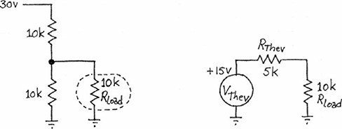
First, let’s make sure Thevenin had it right: let’s make sure his model behaves the way the original circuit does. We found that the 10k, 10k divider from 30 V, which put out 15 V when not loaded, drooped to 10 V under a 10k load; see Fig. 1N.24. Does the model do the same?

Figure 1N.24 Thevenin model and load: droops as original circuit drooped.
Yes, the model droops to the extent the original did: down to 10 V. What the model provides that the original circuit lacked is that single value,  , expressing how droopy/stiff the output is.
If someone changed the value of the load, the Thevenin model would help you to see what droop to expect; if, instead, you didn’t use the model and had to put the two lower resistors in parallel again and recalculate their parallel resistance, you’d take longer to get each answer, and still you might not get a feel for the circuit’s output impedance.
Let’s try using the model on a set of voltage sources that differ only in  . At the same time we can see the effect of an instrument’s input impedance.
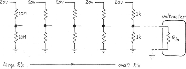
Suppose we have a set of voltage dividers, but dividing a 20 V input by two; see Fig. 1N.25. Let’s assume that we use 1% resistors (value good to  1%):
1%):  is obvious, and is the same in all cases; but
  evidently varies from divider to divider.

Figure 1N.25 Set of similar voltage dividers: same  , differing
  .
.
Suppose now that we try to measure  at the output of each divider. If we measured with a perfect voltmeter, the answer in all cases would be 10 V. (Query: is it 10.000 V? 10.0 V?Footnote 14)
But if we actually perform the measurement, we will see the effect of loading by the  of our imperfect lab voltmeters. Let’s try it with a VOM (“volt-ohm-milliammeter,” the conventional name for the old-fashioned “analog” meter, which gives its answers by deflecting its needle to a degree that forms an analog to the quantity measured), and then with a DVM (“digital voltmeter,” a more recent invention, which usually can measure current and resistance as well as voltage, despite its name; both types sometimes are called simply “multimeters”).
Suppose you poke the several divider outputs, beginning from the right side, where the resistors are  . Here’s a table showing what we found, at three of the dividers:
| R values | measured  | inference |
| 1k | 9.95 | within R tolerance |
| 10k | 9.76 | loading barely apparent |
| 100k | 8.05 | loading obvious |
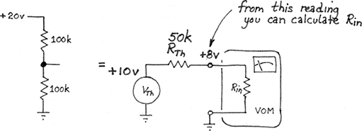
The 8.05 V reading shows such obvious loading – and such a nice round number, if we treat it as “8 V” – that we can use this to calculate the meter’s  without much effort: see Fig. 1N.26.

Figure 1N.26 VOM reading departs from ideal; we can infer  .
.
As usual, one has a choice now, whether to pull out a formula and calculator, or whether to try, instead, to do the calculation “back-of-the-envelope” style. Let’s try the latter method.
First, we know that  is 100k parallel 100k: 50k. Now let’s talk our way to a solution (an approximate solution: we’ll treat the measured
  as just “8 V”):
The meter shows us 8 parts in 10; across the divider’s
(or call it “”) we must be dropping the other 2 parts in 10. The relative sizes of the two resistances are in proportion to these two voltage drops: 8 to 2, so must be : 200k.


If we look closely at the front of the VOM, we’ll find a little notation,

That specification means that if we used the meter on its 1 V scale (that is, if we set things so that an input of 1 V would deflect the needle fully), then the meter would show an input resistance of 20k. In fact, it’s showing us 200k. Does that make sense? It will when you’ve figured out what must be inside a VOM to allow it to change voltage ranges: a set of big series resistors.Footnote 15 Our answer, 200k, is correct when we have the meter set to the 10 V scale, as we do for this measurement.
This is probably a good time to take a quick look at what’s inside a multimeter – VOM or DVM:
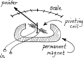
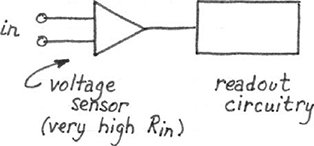
How a meter works: some meter types fundamentally sense current, others sense voltage; see Figs. 1N.27 and 1N.28. Both meter mechanisms, however, can be rigged to measure both quantities, operating as a “multimeter.”

Figure 1N.27 An analog meter senses current in its guts.

Figure 1N.28 A digital meter senses voltage in its innards.
The VOM specification, 20,000 ohms/volt, describes the sensitivity of the meter movement – the guts of the instrument. This movement puts a fairly low ceiling on the VOM’s input resistance at a given range setting.
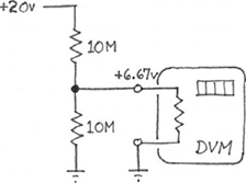
Let’s try the same experiment with a DVM, and let’s suppose we get the following readings:

Again let’s use the case where the droop is obvious; again let’s talk our way to an answer:
This time
is 5M; we’re dropping 2/3 of the voltage across , 1/3 across . So, must be , or 10M.


If we check the datasheet for this particular DVM we find that its  is specified to be “10M, all ranges.” Again our readings make sense.

Figure 1N.29 DVM reading departs from ideal; we can infer  .
.
1N.4.4 VOM versus DVM: a conclusion?
Evidently, the DVM is a better voltmeter, at least in its  – as well as much easier to use. As a current meter, however, it is no better than the VOM: it drops 1/4 V full scale, as the VOM does; it measures current simply by letting it flow through a small resistor; the meter then measures the voltage across that resistor.
1N.4.5 Digression on ground
The concept “ground” (“earth,” in Britain) sounds solid enough. It turns out to be ambiguous. Try your understanding of the term by looking at some cases: see Fig. 1N.30.

Figure 1N.30 Ground in two senses.
Query What is the resistance between points A and B? (Easy, if you don’t think about it too hard.Footnote 16) We know that the ground symbol means, in any event, that the bottom ends of the two resistors are electrically joined. Does it matter whether that point is also tied to the pretty planet we live on? It turns out that it does not.
And where is “ground” in the circuit in Fig. 1N.31?

Figure 1N.31 Ground in two senses, revisited.
Two senses for “Ground”
- “Local ground”
Local ground is what we care about: the common point in our circuit that we arbitrarily choose to call zero volts. Only rarely do we care whether or not that local reference is tied to a spike driven into the earth.
- “Earth ground”
But, be warned, sometimes you are confronted with lines that are tied to world ground – for example, the ground clip on a scope probe, and the “ground” of the breadboards that we use in the lab; then you must take care not to clip the scope ground to, say,
on the breadboard.

For a vivid illustration of “earth” grounding, see an image from Wikipedia: https://LAoE.link/Earth_Ground.html.
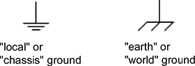
It might be useful to use different symbols for the two senses of ground, and such a convention does exist: see Fig. 1N.32.

Figure 1N.32 Symbols can distinguish the two senses of “ground”.
Unfortunately, this distinction is not widely observed, and in this book as in AoE, we will not maintain this graphical distinction.Footnote 17 Ordinarily, we will use the symbol that Fig. 1N.32 suggests for “local ground.” In the rare case when we intend a connection to “world” ground, we will say so in words, not graphically.
1N.4.6 A rule of thumb for relating to


The voltage dividers whose outputs we tried to measure introduced us to a problem we will see over and over again: some circuit tries to “drive” a load. To some extent, the load changes the output. We need to be able to predict and control this change. To do that, we need to understand, first, the characteristic we call  (this rarely troubles anyone) and, second, the one we have called
  (this one takes longer to get used to). Next time, when we meet frequency-dependent circuits, we will generalize both characteristics to “
 ” and “
 .”
.”
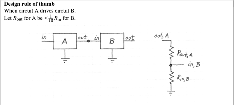
Here we will work our way to another rule of thumb; one that will make your life as designer relatively easy. We start with a Design goal: When circuit A drives circuit B: arrange things so that B loads A lightly enough to cause only insignificant attenuation of the signal. And this goal leads to the rule of thumb in Fig. 1N.33.

Figure 1N.33 Circuit A drives circuit B.
How does this rule get us the desired result? Look at the problem as a familiar voltage divider question. If  is much smaller than
  , then the divider delivers nearly all of the original signal. If the relation is 1:10, then the divider delivers 10/11 of the signal: attenuation is just under 10%, and that’s good enough for our purposes.
We like this arrangement not just because we like big signals. (If that were the only concern, we could always boost the output signal, simply amplifying it.) We like this arrangement above all because it allows us to design circuit-fragments independently: we can design A, then design B, and so on. We need not consider A, B as a large single circuit. That’s good: makes our work of design and analysis lots easier than it would be if we had to treat every large circuit as a unit.
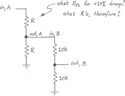
An example, with numbers as in Fig. 1N.34: what  for droop of
  %? What R’s, therefore?

Figure 1N.34 One divider driving another: a chance to apply our rule of thumb.
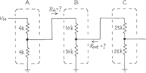
The effects of this rule of thumb become more interesting if you extend this chain: from A and B, on to C: see Fig. 1N.35.

Figure 1N.35 Extending the divider: testing the claim that our rule of thumb lets us consider one circuit fragment at a time.
As we design C, what  should we use for B? Is it just 10k parallel 10k? That’s the answer if we can consider B by itself, using the usual simplifying assumptions: source ideal (
 = 0) and load ideal (
 infinitely large).
But should we be more precise? Should we admit that the upper branch really looks like  : 12k? That’s 20% different. Is our whole scheme crumbling? Are we going to have to look all the way back to the start of the chain, in order to design the next link? Must we, in other words, consider the whole circuit at once, not just the fragment B, as we had hoped?
No. Relax. That 20% error gets diluted to half its value:  for B is 10k parallel 12k, but that’s a shade under 5.5k. So we need not look beyond B. We can, indeed, consider the circuit in the way we had hoped: fragment by fragment.
If this argument has not exhausted you, you might give our claim a further test by looking in the other direction: does C alter B’s input resistance appreciably ( %)? You know the answer, but confirming it would let you check your understanding of our rule of thumb and its effects.
Two important exceptions to our rule of thumb: signals that are currents, and transmission lines
The rule of §1N.4.6 for relating impedances is extremely useful and important. But we should acknowledge two important classes of circuits to which it does not apply:
Signal sources that provide current signals rather than voltage signals. At the moment, this distinction may puzzle you. Yet the distinction between voltage sources – the sort familiar to most of us – versus current sources is substantial and important.Footnote 18
High-frequency circuits where the signal paths must be treated as “transmission lines” (see App-endix C).
Only at frequencies above what we will use in this course do such effects become apparent. These are frequencies (or frequency components, since “steep” waveform edges include high-frequency components, as Fourier teaches – see Chapter 3N) where the period of a signal is comparable to the time required for that signal to travel to the end of its path. For example, a six-foot cable’s propagation time would be about 9 ns, the period of a
sinusoid. Square waves are still more troublesome; one at even a few MHz would include quite a strong component at that frequency, and this component would be distorted by such a cable if we did not take care to “terminate” it properly. In fact, these calculations understate the difficulties; a round-trip path length greater than about 1/10th wavelength calls for termination.

AoE §H.1
We don’t want you to worry, right now, about these two points. Signals as currents are unusual in this course, and in this course you are not likely to confront transmission-line problems. But be warned that you will meet these later, if you begin to work with signals at higher frequencies.
1N.5 AoE reading
This is the first instance in which we’ve tried to steer you toward particular sections of The Art of Electronics. That book is, of course a sibling (or is it the mother?) of the book you are reading. You should not consider the readings listed below to be required. But if you are proceeding by using the two books in parallel, these are the sections we consider most relevant.
Readings:
Chapter 1, §§1.1–1.3.2.
Appendix C on resistor types: resistor color code and precision resistors.
Appendix H on transmission lines.
Problems:
Problems in text.
Exercises 1.37, 1.38.