


1. Model equations and assumptions
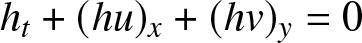
In this work, we study the shallow water wave (or Saint-Venant) model:
 \begin{align}
h_t + (hu)_x + (hv)_y & = 0
\end{align}
\begin{align}
h_t + (hu)_x + (hv)_y & = 0
\end{align}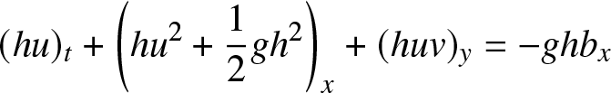 \begin{align}
(hu)_t + \left( hu^2 + \frac{1}{2}gh^2 \right)_x + (huv)_y & = - g h b_x
\end{align}
\begin{align}
(hu)_t + \left( hu^2 + \frac{1}{2}gh^2 \right)_x + (huv)_y & = - g h b_x
\end{align}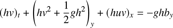 \begin{align}
(hv)_t + \left( hv^2 + \frac{1}{2} gh^2\right)_y + (huv)_x & = - g h b_y
\end{align}
\begin{align}
(hv)_t + \left( hv^2 + \frac{1}{2} gh^2\right)_y + (huv)_x & = - g h b_y
\end{align} where g = 9.81 is the gravitational acceleration,  $h(x,y,t)$ denotes the depth, $u(x,y,t) and v(x,y,t)$ denotes the horizontal velocity components and
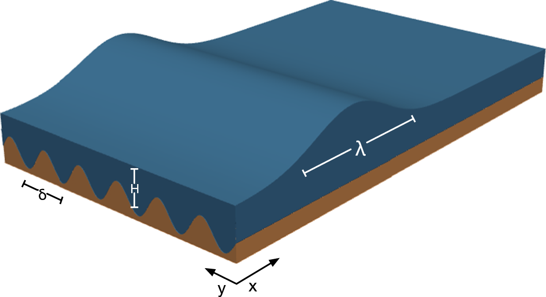
  $b(x,y)$ is the bottom elevation (bathymetry). As illustrated in Figure 1, we are interested in the behaviour of waves propagating over bathymetry that does not depend on x and is periodic in y with period δ:
 \begin{equation*}
b(y+\delta) = b(y).
\end{equation*}
\begin{equation*}
b(y+\delta) = b(y).
\end{equation*}Geometry of the problem studied herein. The bathymetry b(y) is shown in brown and repeats periodically with period δ in the y direction. The regime studied herein is that for which  $\lambda \gg \delta$.
We focus on the propagation of initially planar waves travelling parallel to the x-axis:
 \begin{align}
\eta(x,y,0) & = \eta_0(x) & u(x,y,0) & = u_0(x) & v(x,y,0) = 0.
\end{align}
\begin{align}
\eta(x,y,0) & = \eta_0(x) & u(x,y,0) & = u_0(x) & v(x,y,0) = 0.
\end{align} Here  $\eta=h+b$ is the surface elevation. Due to symmetry, this can equivalently be seen as a model for waves in a non-rectangular channel with frictionless walls [Reference Quezada de Luna and Ketcheson13, Section 1.2], a problem which has also been studied (using other water wave models) for instance in [Reference Chassagne, Filippini, Ricchiuto and Bonneton3, Reference Peregrine11, Reference Teng and Theodore15].
It has been shown that linear plane waves travelling parallel to variations in the medium of propagation exhibit effective dispersion if there is variation in the sound speed [Reference Quezada de Luna and Ketcheson12]. For nonlinear shallow water waves, this effective dispersion can lead to the formation of solitary waves even though the equations themselves are non-dispersive [Reference Quezada de Luna and Ketcheson13]. In the latter work, a partially heuristic constant-coefficient KdV-type model was shown to approximate the behaviour of such waves. We refer also to [Reference Chassagne, Filippini, Ricchiuto and Bonneton3, Reference Gavrilyuk and Ricchiuto5] for the development of a similar model and comparison with experiments. In the present work, we develop a more accurate and detailed effective model for these waves. We apply multiple-scale perturbation analysis to show that these waves are described, to leading order, by a Boussinesq-type system with a dispersive coefficient depending on the bathymetry. The effective model describes the full two-dimensional structure of the waves and is shown to be in agreement with detailed numerical simulations. The main novel contributions of this work are:
• A constant-coefficient 1D model equation whose solution accurately approximates the average of the 2D variable-coefficient problem;
• a computational exploration of solutions to the problem using both finite volume and pseudospectral methods;
• analysis and computation of the solitary waves that naturally arise as typical solutions in this problem;
• an analytic approximation to those solitary waves.
The perturbation approach used here is based on that developed by Yong and coauthors [Reference LeVeque and Yong9, Reference Yong and Kevorkian16]. We have conducted a similar analysis for plane waves propagating perpendicular to the bathymetric variation; in that case, the problem can be reduced to one horizontal dimension [Reference Ketcheson, Lóczi and Russo6]. In the one-dimensional setting, effective dispersion is caused by wave reflection, whereas in the setting of the present work, it is caused by propagation perpendicular to the direction of bathymetric variation and may be described as the result of diffraction [Reference Quezada de Luna and Ketcheson12]. It is also reasonable to describe this behaviour as the result of refraction since the deep and shallow regions have different characteristic wave speeds. Compared to the model derived in [Reference Quezada de Luna and Ketcheson13], the model derived herein provides a more detailed (two-dimensional) and accurate description of solutions, in particular, for larger waves and longer times. In principle, the technique used here could be carried out to higher orders in order to obtain an even more accurate description.
Throughout the paper, we use dimensional quantities with SI units, so lengths are measured in meters and time in seconds. The code to reproduce the calculations and figures in this work is available online.Footnote 1
The rest of the paper is organized as follows. In Section 2, we perform a multiple-scale analysis leading to an effective medium equation for the waves of interest; the main result is equation (23), which describes the evolution of such waves after averaging over the y-dimension. In Section 3, we compare solutions of the effective equations with those of the original variable-bathymetry system (1). In Section (4), we investigate the shape of these two-dimensional solitary waves, comparing the predictions of the multiple-scale analysis with the results of numerical experiments. Some conclusions are provided in Section 5.
2. Multiple-scale analysis
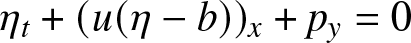
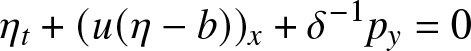
The choice of primary variables is a key decision in perturbation analysis of systems like the one considered here. One usually works with the conserved variables  $(h, hu, hv)$ in order to include weak solutions, but here we are interested in strong solutions. Since we seek to derive a system of equations describing the variation of the solution over long-length scales, we prefer to use quantities that do not necessarily vary on the periodic microscale for near-equilibrium solutions (see e.g. [Reference Ketcheson, Lóczi and Russo6, Reference LeVeque and Yong9] for other examples). In the present setting, this indicates that one should use the surface elevation η rather than h and the y-momentum p = hv rather than v. After some trial and error, we found it best to rewrite (1) in terms of $(\eta,u,p)$:
 \begin{align}
\eta_t + (u(\eta-b))_x + p_y & = 0
\end{align}
\begin{align}
\eta_t + (u(\eta-b))_x + p_y & = 0
\end{align}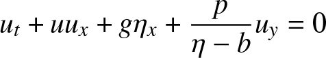 \begin{align}
u_t + u u_x + g \eta_x + \frac{p}{\eta-b} u_y & = 0
\end{align}
\begin{align}
u_t + u u_x + g \eta_x + \frac{p}{\eta-b} u_y & = 0
\end{align}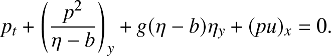 \begin{align}
p_t + \left( \frac{p^2}{\eta-b}\right)_y + g(\eta-b)\eta_y + (p u)_x & = 0.
\end{align}
\begin{align}
p_t + \left( \frac{p^2}{\eta-b}\right)_y + g(\eta-b)\eta_y + (p u)_x & = 0.
\end{align}Note that it is not important to write the equations in conservation form since we are primarily interested in strong solutions to this system.
A second critical choice is that of a small parameter. We assume that the wavelength of the typical waves we are interested in is long relative to the period δ of the bathymetry. We perform a change of variables, by introducing  $\tilde{y} = y/\delta$, so now $b(y) = b(\tilde{y}\delta) = \tilde{b}(\tilde{y})$, with $\tilde{b}$ a 1-periodic function, and $\partial/\partial y = \delta^{-1}\partial/\partial \tilde{y}$. We next rewrite the equations in the new coordinates $(x,\tilde{y},t)$ and suppress the tildes to obtain
 \begin{align}
\eta_t + (u(\eta-b))_x + \delta^{-1} p_y & = 0
\end{align}
\begin{align}
\eta_t + (u(\eta-b))_x + \delta^{-1} p_y & = 0
\end{align}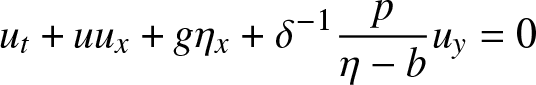 \begin{align}
u_t + u u_x + g \eta_x + \delta^{-1} \frac{p}{\eta-b} u_y & = 0
\end{align}
\begin{align}
u_t + u u_x + g \eta_x + \delta^{-1} \frac{p}{\eta-b} u_y & = 0
\end{align}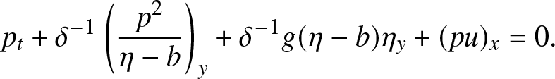 \begin{align}
p_t + \delta^{-1} \left( \frac{p^2}{\eta-b}\right)_y + \delta^{-1} g(\eta-b)\eta_y + (p u)_x & = 0.
\end{align}
\begin{align}
p_t + \delta^{-1} \left( \frac{p^2}{\eta-b}\right)_y + \delta^{-1} g(\eta-b)\eta_y + (p u)_x & = 0.
\end{align} We now look for solutions which are small perturbations, of  $O(\delta)$, of the lake at rest given by $(\eta,u,p) = (\eta^0,0,0)$. We emphasize that η 0 denotes the unperturbed surface elevation while $\eta_0(x,y)$ denotes the surface elevation at the initial time. Furthermore, since the problem is invariant under a vertical coordinate shift, we can without loss of generality take $\eta^0=0$, which we will do in the numerical experiments.
We assume the quantities  $\eta, u, p$ can be written as power series in δ with the form
 \begin{align}
\eta - \eta^0 & = \delta \eta^1(x,y,t) + \delta^2 \eta^2(x,y,t) + \cdots
\end{align}
\begin{align}
\eta - \eta^0 & = \delta \eta^1(x,y,t) + \delta^2 \eta^2(x,y,t) + \cdots
\end{align} \begin{align}
u & = \delta u^1(x,y,t) + \delta^2 u^2(x,y,t) + \cdots
\end{align}
\begin{align}
u & = \delta u^1(x,y,t) + \delta^2 u^2(x,y,t) + \cdots
\end{align} \begin{align}
p & = \delta p^1(x,y,t) + \delta^2 p^2(x,y,t) + \cdots.
\end{align}
\begin{align}
p & = \delta p^1(x,y,t) + \delta^2 p^2(x,y,t) + \cdots.
\end{align} Here and throughout this section, superscripts on  $\eta, u$ and p denote indices of the asymptotic expansion (5). When needed, we shall adopt parentheses to denote the exponentiation of these quantities. All functions are assumed to be periodic in y with period 1. In what follows, we use
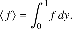
  $\langle\cdot\rangle$ to denote quantities that are averaged with respect to y, i.e. for any function $f(x,y,t)$ we have
 \begin{equation*}
\langle\ f \rangle = \int_0^1 f\, dy.
\end{equation*}
\begin{equation*}
\langle\ f \rangle = \int_0^1 f\, dy.
\end{equation*} Notice that if f does not depend on y then  $f = \langle\ f \rangle$, and that $\langle\cdot\rangle$ commutes with x and t derivatives, i.e. $\langle\ f \rangle_t = \langle\ f_t \rangle$ and $\langle\ f \rangle_x = \langle\ f_x \rangle$. Throughout the paper, we denote by
 \begin{equation*}H(y)\equiv \eta^0-b(y)\end{equation*}
the unperturbed water depth.
Next, we substitute (5) into (4) and equate terms at each power of δ.
2.1.  ${\mathcal O}(\delta^0)$

First, we collect all terms proportional to δ 0. The expansion of (4b) does not contain any such terms. From the expansion of (4a), we obtain  $
p^1_y=0
$ while (4c) gives
$
p^1_y=0
$ while (4c) gives
 \begin{equation*}
g H(y)\eta^1_y = 0
\end{equation*}
\begin{equation*}
g H(y)\eta^1_y = 0
\end{equation*}From these relations, we deduce that p 1 and η 1 do not depend on y.
2.2.
${\mathcal O}(\delta^1)$

Next, collecting terms proportional to δ 1, we obtain
 \begin{align}
\eta^1_t + H u^1_x + p^2_y & = 0
\end{align}
\begin{align}
\eta^1_t + H u^1_x + p^2_y & = 0
\end{align} \begin{align}
u^1_t + g \eta^1_x + \frac{p^1u^1_y}{H} & = 0
\end{align}
\begin{align}
u^1_t + g \eta^1_x + \frac{p^1u^1_y}{H} & = 0
\end{align}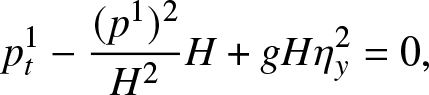 \begin{align}
p^1_t - \frac{(p^1)^2}{H^2} H + g H \eta^2_y & = 0,
\end{align}
\begin{align}
p^1_t - \frac{(p^1)^2}{H^2} H + g H \eta^2_y & = 0,
\end{align} We have concluded already that η 1 is independent of y, and we assume that  $u(x,y,0)$ is independent of y, so ut is initially independent of y. Equation (6b) shows that it will remain so for all time. Now we average these equations with respect to y – i.e. we integrate (6) with respect to y over one period, noting that the average of any y-derivative is zero. Since η 1 is independent of y, Equation (6b) implies that $u^1_t$ is also independent of y. Since we assume that $u(x,y,0)$ is independent of y we deduce further that u 1 does not depend on y, so we obtain
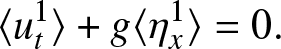 \begin{equation*}
\langle u^1_t \rangle + g \langle \eta^1_x \rangle = 0.
\end{equation*}
\begin{equation*}
\langle u^1_t \rangle + g \langle \eta^1_x \rangle = 0.
\end{equation*} In order to make the notation more uniform, when considering the evolution of averages in y, for any quantity w independent of y we shall indicate it as  $\langle w \rangle$ even if $\langle w \rangle=w$.
Solving (6c) for  $\eta^2_y$ and averaging the result gives
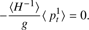 \begin{equation*}
-\frac{\langle H^{-1}\rangle}{g}
\langle\ p^1_t \rangle = 0.
\end{equation*}
\begin{equation*}
-\frac{\langle H^{-1}\rangle}{g}
\langle\ p^1_t \rangle = 0.
\end{equation*} Since we assume  $p(x,y,0)=0$, this implies $p^1 = 0$. Returning to (6c), this in turn implies $\eta^2_y=0$, so
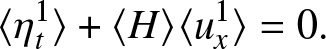
  $\eta^2 = \langle \eta^2 \rangle$. Averaging (6a) in y gives
 \begin{align*}
\langle \eta^1_t \rangle + \langle H \rangle \langle u^1_x \rangle & = 0.
\end{align*}
\begin{align*}
\langle \eta^1_t \rangle + \langle H \rangle \langle u^1_x \rangle & = 0.
\end{align*}Taking together these averaged equations, we have the system
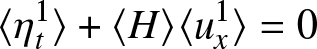 \begin{align}
\langle \eta^1_t \rangle + \langle H \rangle\langle u^1_x \rangle & = 0
\end{align}
\begin{align}
\langle \eta^1_t \rangle + \langle H \rangle\langle u^1_x \rangle & = 0
\end{align}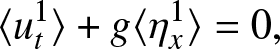 \begin{align}
\langle u^1_t \rangle + g \langle \eta^1_x \rangle & = 0,
\end{align}
\begin{align}
\langle u^1_t \rangle + g \langle \eta^1_x \rangle & = 0,
\end{align} which is simply the linear wave equation with wave speed  $c=\sqrt{g\langle H \rangle}$. It is interesting to note that here the average depth appears in the wave speed, whereas the harmonic average appears for waves propagating perpendicular to the lines of constant bathymetry (see [Reference Ketcheson, Lóczi and Russo6] and also [Reference Quezada de Luna and Ketcheson12]).
We can further manipulate (6a) to obtain an expression for p 2, the leading-order term in the y-momentum. Subtracting (8a) from (6a) we obtain
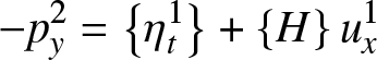 \begin{equation*}
-p^2_y = \left\{{\eta^1_t}\right\} + \left\{{H}\right\}u^1_x
\end{equation*}
\begin{equation*}
-p^2_y = \left\{{\eta^1_t}\right\} + \left\{{H}\right\}u^1_x
\end{equation*}where, for any function f, we denote by
 \begin{equation*}
\left\{\,f\right\} \equiv f - \langle\ f \rangle
\end{equation*}
\begin{equation*}
\left\{\,f\right\} \equiv f - \langle\ f \rangle
\end{equation*} the fluctuating part of f. Considering that  $\eta^1=\langle \eta^1 \rangle$ we have
 \begin{equation}
p^2_y = -\left\{{H}\right\}u^1_x =
{-\left\{{H}\right\}\langle u^1_x \rangle }
\end{equation}
\begin{equation}
p^2_y = -\left\{{H}\right\}u^1_x =
{-\left\{{H}\right\}\langle u^1_x \rangle }
\end{equation}Integrating Equation (9) and imposing that the two sides have the same average, one gets
 \begin{equation}
p^2(x,y,t) = -\unicode{x27E6} H \unicode{x27E7} \langle u^1_x \rangle + \langle\ p^2 \rangle
\end{equation}
\begin{equation}
p^2(x,y,t) = -\unicode{x27E6} H \unicode{x27E7} \langle u^1_x \rangle + \langle\ p^2 \rangle
\end{equation} where, for any function of f(y),  $\unicode{x27E6} f \unicode{x27E7}$ denotes the integral of the fluctuating part of f:
 \begin{equation*}
\unicode{x27E6}\ f \unicode{x27E7} = \int_s^y (\,f(\xi)-\langle\ f \rangle) d\xi \ \ \text{where}\ s\ \text{is chosen so that } \langle \unicode{x27E6}\ f \unicode{x27E7} \rangle = 0.
\end{equation*}
\begin{equation*}
\unicode{x27E6}\ f \unicode{x27E7} = \int_s^y (\,f(\xi)-\langle\ f \rangle) d\xi \ \ \text{where}\ s\ \text{is chosen so that } \langle \unicode{x27E6}\ f \unicode{x27E7} \rangle = 0.
\end{equation*}2.3.
${\mathcal O}(\delta^2)$

Collecting terms proportional to δ 2, we obtain
 \begin{align}
-p^3_y & = \eta^2_t + Hu^2_x + (\langle \eta^1 \rangle \langle u^1 \rangle)_x
\end{align}
\begin{align}
-p^3_y & = \eta^2_t + Hu^2_x + (\langle \eta^1 \rangle \langle u^1 \rangle)_x
\end{align} \begin{align}
0 & = u^2_t + \langle u^1 \rangle \langle u^1_x \rangle + g \langle \eta^2_x \rangle
\end{align}
\begin{align}
0 & = u^2_t + \langle u^1 \rangle \langle u^1_x \rangle + g \langle \eta^2_x \rangle
\end{align} \begin{align}
-g \eta^3_y & = \frac{1}{H}(\,p^2_t + g \langle \eta^1 \rangle \langle \eta^2_y \rangle) = \frac{1}{H}(-\unicode{x27E6} H \unicode{x27E7}\langle u^1_{xt} \rangle + \langle\ p^2 \rangle_t).
\end{align}
\begin{align}
-g \eta^3_y & = \frac{1}{H}(\,p^2_t + g \langle \eta^1 \rangle \langle \eta^2_y \rangle) = \frac{1}{H}(-\unicode{x27E6} H \unicode{x27E7}\langle u^1_{xt} \rangle + \langle\ p^2 \rangle_t).
\end{align} In the last line, we have used that η 2 is independent of y and Equation (10). The only term in (11b) that could depend on y is  $u^2_t$, so it must be independent of y; i.e. $u^2 = \langle u^2 \rangle(x,t)$. Thus we have
 \begin{align}
\langle u^2_t \rangle + \langle u^1 \rangle \langle u^1_x \rangle + g \langle \eta^2_x \rangle & = 0.
\end{align}
\begin{align}
\langle u^2_t \rangle + \langle u^1 \rangle \langle u^1_x \rangle + g \langle \eta^2_x \rangle & = 0.
\end{align}Taking the average of (11a) gives
 \begin{align}
\langle \eta^2_t \rangle + \langle H \rangle\langle u^2_x \rangle + (\langle \eta^1 \rangle \langle u^1 \rangle)_x = 0.
\end{align}
\begin{align}
\langle \eta^2_t \rangle + \langle H \rangle\langle u^2_x \rangle + (\langle \eta^1 \rangle \langle u^1 \rangle)_x = 0.
\end{align}Subtracting this from (11a) and integrating in y, we get
 \begin{align}
p^3(x,y,t) & = -\unicode{x27E6} H \unicode{x27E7}\langle u^2_x \rangle + \langle\ p^3 \rangle.
\end{align}
\begin{align}
p^3(x,y,t) & = -\unicode{x27E6} H \unicode{x27E7}\langle u^2_x \rangle + \langle\ p^3 \rangle.
\end{align} For simplicity, we now specialize our analysis to bathymetry profiles for which  $\langle H^{-1} \unicode{x27E6} H \unicode{x27E7}\rangle=0$, which holds for instance for the piecewise-constant or sinusoidal bathymetries studied below (see [Reference Ketcheson, Lóczi and Russo6], Proposition 5). Then taking the average of (11c), we find that $\langle\ p^2 \rangle_t=0$. Since $p^2(x,y,0) = 0$, it follows that $\langle\ p^2 \rangle = 0$. Then integrating (11c) in y yields
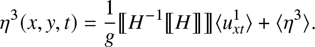
 \begin{align}
\eta^3(x,y,t) = \frac{1}{g} \unicode{x27E6} H^{-1} \unicode{x27E6} H \unicode{x27E7} \unicode{x27E7} \langle u^{1}_{xt} \rangle + \langle \eta^{3} \rangle.
\end{align}
\begin{align}
\eta^3(x,y,t) = \frac{1}{g} \unicode{x27E6} H^{-1} \unicode{x27E6} H \unicode{x27E7} \unicode{x27E7} \langle u^{1}_{xt} \rangle + \langle \eta^{3} \rangle.
\end{align}Based on what we have determined up to this point, we can write the series (5) more simply as
 \begin{align}
\eta - \eta^0 & = \delta \eta^1(x,t) + \delta^2 \eta^2(x,t) + \cdots
\end{align}
\begin{align}
\eta - \eta^0 & = \delta \eta^1(x,t) + \delta^2 \eta^2(x,t) + \cdots
\end{align} \begin{align}
u & = \delta u^1(x,t) + \delta^2 u^2(x,t) + \cdots
\end{align}
\begin{align}
u & = \delta u^1(x,t) + \delta^2 u^2(x,t) + \cdots
\end{align} \begin{align}
p & = \delta^2 p^2(x,y,t) + \cdots.
\end{align}
\begin{align}
p & = \delta^2 p^2(x,y,t) + \cdots.
\end{align} Let  $\overline{\eta} = \delta^{-1}\langle \eta-\eta^0 \rangle$ and $\overline{u}=\delta^{-1}\langle u \rangle$. By adding δ times (8a) to δ 2 times (13), we get an approximate equation for the evolution of $\overline{\eta}$:
 \begin{align}
\delta\left(\overline{\eta}_t + \langle H \rangle\overline{u}_x\right) + \delta^2(\overline{\eta} \ \overline{u})_x & = {\mathcal O}(\delta^3).
\end{align}
\begin{align}
\delta\left(\overline{\eta}_t + \langle H \rangle\overline{u}_x\right) + \delta^2(\overline{\eta} \ \overline{u})_x & = {\mathcal O}(\delta^3).
\end{align} Similarly, by adding δ times (8b) to δ 2 times (12), we get an approximate equation for the evolution of  $\overline{u}$:
 \begin{align}
\delta\left(\overline{u}_t + g\overline{\eta}_x\right) + \delta^2(\overline{u} \ \overline{u}_x) & = {\mathcal O}(\delta^3).
\end{align}
\begin{align}
\delta\left(\overline{u}_t + g\overline{\eta}_x\right) + \delta^2(\overline{u} \ \overline{u}_x) & = {\mathcal O}(\delta^3).
\end{align}We see that up to this order, the y-averaged variables satisfy a nonlinear first-order hyperbolic system. We proceed with the analysis at the next order, where we expect to see dispersive terms.
2.4.
${\mathcal O}(\delta^3)$

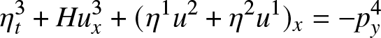
Collecting terms proportional to δ 3, we obtain
 \begin{align}
\eta^3_t + H u^3_x + (\eta^1u^2 + \eta^2 u^1)_x & = -p^4_y
\end{align}
\begin{align}
\eta^3_t + H u^3_x + (\eta^1u^2 + \eta^2 u^1)_x & = -p^4_y
\end{align} \begin{align}
u^3_t + (u^1 u^2)_x + \unicode{x27E6} H^{-1}\unicode{x27E6} H \unicode{x27E7} \unicode{x27E7} u^1_{xtx} + g \eta^3_x & = 0
\end{align}
\begin{align}
u^3_t + (u^1 u^2)_x + \unicode{x27E6} H^{-1}\unicode{x27E6} H \unicode{x27E7} \unicode{x27E7} u^1_{xtx} + g \eta^3_x & = 0
\end{align} \begin{align}
\frac{1}{H} \left( p^3_t - H^{-2}(\,p^2)^2 H' + 2 H^{-1} p^2 p^2_y + g \eta^1 \eta^3_y + (\,p^2 u^1)_x \right) & = -g \eta^4_y.
\end{align}
\begin{align}
\frac{1}{H} \left( p^3_t - H^{-2}(\,p^2)^2 H' + 2 H^{-1} p^2 p^2_y + g \eta^1 \eta^3_y + (\,p^2 u^1)_x \right) & = -g \eta^4_y.
\end{align}Averaging (18a) yields
 \begin{align}
\langle \eta^3 \rangle_t + \langle H u^3 \rangle_x + (\langle \eta^1 \rangle \langle u^2 \rangle + \langle \eta^2 \rangle \langle u^1 \rangle)_x & = 0.
\end{align}
\begin{align}
\langle \eta^3 \rangle_t + \langle H u^3 \rangle_x + (\langle \eta^1 \rangle \langle u^2 \rangle + \langle \eta^2 \rangle \langle u^1 \rangle)_x & = 0.
\end{align} Since u 3 may depend on y, we must work directly with the average  $\langle Hu^3 \rangle$. We therefore multiply (18b) by H before averaging, to obtain
 \begin{align*}
\langle Hu^3 \rangle_t + \langle H \rangle(\langle u^1 \rangle \langle u^2 \rangle)_x - \mu \langle u^1_{xxt}\rangle + g \langle H \rangle\langle \eta^3_x \rangle & = 0.
\end{align*}
\begin{align*}
\langle Hu^3 \rangle_t + \langle H \rangle(\langle u^1 \rangle \langle u^2 \rangle)_x - \mu \langle u^1_{xxt}\rangle + g \langle H \rangle\langle \eta^3_x \rangle & = 0.
\end{align*}where
 \begin{align*}
\mu & = -\langle H \unicode{x27E6} H^{-1} \unicode{x27E6} H \unicode{x27E7} \unicode{x27E7} \rangle = \langle H^{-1} (\unicode{x27E6} H \unicode{x27E7})^2\rangle.
\end{align*}
\begin{align*}
\mu & = -\langle H \unicode{x27E6} H^{-1} \unicode{x27E6} H \unicode{x27E7} \unicode{x27E7} \rangle = \langle H^{-1} (\unicode{x27E6} H \unicode{x27E7})^2\rangle.
\end{align*} The last equality comes from the general property  $\langle a\unicode{x27E6} b \unicode{x27E7} \rangle =- \langle \unicode{x27E6} a \unicode{x27E7} b\rangle$ for all functions a(y) b(y) [Reference Yong and Kevorkian16, Appendix A] (here we take $a=H, b=H^{-1}\unicode{x27E6} H \unicode{x27E7}$).
Introducing  $\langle q^j \rangle = \langle Hu^j \rangle$, this is
 \begin{align}
\langle q^3 \rangle_t + \langle H \rangle^{-1}(\langle q^1 \rangle \langle q^2 \rangle)_x - \langle H \rangle^{-1}\mu \langle q^1_{xxt}\rangle + g \langle H \rangle\langle \eta^3_x \rangle & = 0.
\end{align}
\begin{align}
\langle q^3 \rangle_t + \langle H \rangle^{-1}(\langle q^1 \rangle \langle q^2 \rangle)_x - \langle H \rangle^{-1}\mu \langle q^1_{xxt}\rangle + g \langle H \rangle\langle \eta^3_x \rangle & = 0.
\end{align} Here we made use of the fact that u 1 and u 2 are independent of y. Averaging (18c), after a number of tedious calculations, yields  $\langle\ p^3 \rangle = 0$.
2.5. Governing equations for averaged variables
Let  $\overline{q} = \sum_j \delta^{j-1} \langle q^j \rangle$. We now add $\delta\langle H \rangle$ times (8b), plus $\delta^2\langle H \rangle$ times (12), plus δ 3 times (22). This gives
 \begin{align}
\delta( \overline{q}_t + g\langle H \rangle\overline{\eta}_x) + \delta^2 \langle H \rangle^{-1} \overline{q} \ \overline{q}_x & = \delta^3 \langle H \rangle^{-1} \mu \overline{q}_{xxt} + {\mathcal O}(\delta^4)
\end{align}
\begin{align}
\delta( \overline{q}_t + g\langle H \rangle\overline{\eta}_x) + \delta^2 \langle H \rangle^{-1} \overline{q} \ \overline{q}_x & = \delta^3 \langle H \rangle^{-1} \mu \overline{q}_{xxt} + {\mathcal O}(\delta^4)
\end{align}Similarly, adding δ times (8a) with δ 2 times (13) with δ 3 times (19) results in
 \begin{align*}
\delta(\overline{\eta}_t + \overline{q}_x) + \delta^2 \langle H \rangle^{-1}(\overline{\eta} \ \overline{q})_x & = {\mathcal O}(\delta^4).
\end{align*}
\begin{align*}
\delta(\overline{\eta}_t + \overline{q}_x) + \delta^2 \langle H \rangle^{-1}(\overline{\eta} \ \overline{q})_x & = {\mathcal O}(\delta^4).
\end{align*}It turns out that this system is identical to the so-called classical Boussinesq system that was originally derived as a model for long-wavelength waves over a flat-bottom channel. Remarkably, here it has arisen in a completely different way, starting from the non-dispersive Saint-Venant system, and with dispersion arising purely from the effect of a non-flat bottom. In the present context, the coefficients of the convective and dispersive terms depend on the bathymetry b(y) and so their relative magnitude can be quite different based on the chosen geometry. This system is known to be well-posed [Reference Amick1, Reference Bona, Chen and Saut2, Reference Schonbek14].
In principle the asymptotic analysis can be carried out to higher order, deriving additional high-order effective dispersive terms. Of course, it should be kept in mind that by starting from the Saint-Venant system (1) we have already discarded certain higher-order effects that might compete with or dominate the additional terms obtained through such an analysis. This will depend on the relative size of the shallowness parameter  $H/\lambda$ and the bathymetry parameter $\delta/\lambda$.
2.6. Two-dimensional wave structure
In addition to providing an effective model for wave propagation in terms of y-averaged quantities, the homogenization process also allows us to determine the variation of solutions with respect to the y coordinate.
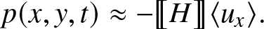
For the y-momentum, from equations (10) and (14) together with the fact that  $\langle p \rangle=0$ we immediately obtain that the variation in y is proportional to $\unicode{x27E6} H \unicode{x27E7}$:
 \begin{align}
p(x,y,t) & \approx -\unicode{x27E6} H \unicode{x27E7} \langle u_x \rangle.
\end{align}
\begin{align}
p(x,y,t) & \approx -\unicode{x27E6} H \unicode{x27E7} \langle u_x \rangle.
\end{align} From (8b) we have that  $\langle u^1_t \rangle \approx -g\langle \eta^1_x \rangle$, and therefore $\langle u^1_{xt \rangle} \approx -g\langle \eta^1_{xx }\rangle$, so then from (15) we obtain
 \begin{align*}
\eta(x,y,t) - \eta^0 & = \delta \langle \eta^1 \rangle(x,t) + \delta^2 \langle \eta^2 \rangle(x,t) + \delta^3(\langle \eta^3 \rangle(x,t) - \unicode{x27E6} H^{-1}\unicode{x27E6} H \unicode{x27E7} \unicode{x27E7} \langle \eta^1_{xx}\rangle) + {\mathcal O}(\delta^4),
\end{align*}
\begin{align*}
\eta(x,y,t) - \eta^0 & = \delta \langle \eta^1 \rangle(x,t) + \delta^2 \langle \eta^2 \rangle(x,t) + \delta^3(\langle \eta^3 \rangle(x,t) - \unicode{x27E6} H^{-1}\unicode{x27E6} H \unicode{x27E7} \unicode{x27E7} \langle \eta^1_{xx}\rangle) + {\mathcal O}(\delta^4),
\end{align*}or equivalently
 \begin{align}
\eta(x,y,t) \approx \langle \eta \rangle(x,t) - \delta^2\unicode{x27E6} H^{-1}\unicode{x27E6} H \unicode{x27E7} \unicode{x27E7} \langle \eta_{xx}\rangle,
\end{align}
\begin{align}
\eta(x,y,t) \approx \langle \eta \rangle(x,t) - \delta^2\unicode{x27E6} H^{-1}\unicode{x27E6} H \unicode{x27E7} \unicode{x27E7} \langle \eta_{xx}\rangle,
\end{align} showing that the leading variation with respect to y is proportional to  $\unicode{x27E6} H^{-1}\unicode{x27E6} H \unicode{x27E7} \unicode{x27E7} \langle \eta_{xx}\rangle$.
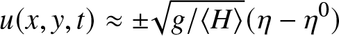
Finally, from the leading-order linear system (8), looking for simple waves, we have that
 \begin{align}
u(x,y,t) & \approx \pm \sqrt{g/\langle H \rangle} (\eta - \eta^0)
\end{align}
\begin{align}
u(x,y,t) & \approx \pm \sqrt{g/\langle H \rangle} (\eta - \eta^0)
\end{align}with the plus sign for right-going waves and minus for left-going waves.
3. Numerical comparison
In this section, we explore the accuracy of the homogenized approximation by comparing its numerical solutions to numerical solutions of the original system (1). We start by discussing the methods adopted for the numerical solution of both the original system (1) and the homogenized system (23).
3.1. Numerical discretization of the homogenized equations
We solve the homogenized equations (23) with a Fourier pseudospectral discretization in space and explicit 3-stage 3rd-order SSP Runge–Kutta integration in time. We can write this system as
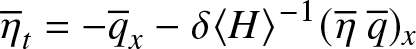 \begin{align}
\overline{\eta}_t & = - \overline{q}_x - \delta \langle H \rangle^{-1} (\overline{\eta} \ \overline{q})_x
\end{align}
\begin{align}
\overline{\eta}_t & = - \overline{q}_x - \delta \langle H \rangle^{-1} (\overline{\eta} \ \overline{q})_x
\end{align} \begin{align}
\overline{q}_t & = -(1-\delta^2 \langle H \rangle^{-1} \mu \partial_x^2)^{-1} \left(g \langle H \rangle\overline{\eta}_x + \delta \langle H \rangle^{-1} \overline{q} \ \overline{q}_x \right)
\end{align}
\begin{align}
\overline{q}_t & = -(1-\delta^2 \langle H \rangle^{-1} \mu \partial_x^2)^{-1} \left(g \langle H \rangle\overline{\eta}_x + \delta \langle H \rangle^{-1} \overline{q} \ \overline{q}_x \right)
\end{align} We discretize in the standard pseudospectral way and then apply the inverse elliptic operator  $(1-\delta^2 \langle H \rangle^{-1} \mu \partial_x^2)^{-1}$ in Fourier space, which does not require the solution of any algebraic system. We can therefore integrate the pseudospectral semi-discretization of (28) efficiently with an explicit Runge–Kutta method.
For the spatial domain, we take  $x\in[-L,L]$ where L is chosen large enough that the waves do not reach the boundaries before the final time.
3.2. Numerical methods for the variable-bathymetry shallow water system
For the solution of the first-order variable-coefficient hyperbolic shallow water system (1), we use two different approaches, depending on the nature of the bathymetry. Accurate solution of this system is much more expensive as it requires a much finer spatial mesh, in order to resolve the bathymetric variation and its effects, and it requires the solution of a problem in two space dimensions. applied at x = 0.
For piecewise-constant (discontinuous) bathymetry, we use the finite volume code Clawpack [Reference LeVeque8, Reference Mandli, Ahmadia, Berger, Calhoun, George, Hadjimichael, Ketcheson, Lemoine and LeVeque10], employing the SharpClaw algorithm, based on 5th-order WENO reconstruction in space and 4th-order Runge–Kutta integration in time [Reference Ketcheson, Parsani and LeVeque7]. This algorithm is well adapted to handle the lack of regularity in both the coefficients and the solution. For continuous bathymetry, we again use the Clawpack code and we also compute the solution with a standard Fourier collocation pseudospectral method in space and 4th-order Runge–Kutta integration in time. Ordinarily one would avoid the use of spectral methods for a first-order hyperbolic problem, but since we focus on scenarios in which shocks do not form, this method performs well and is more efficient than a finite volume discretization, as long as the bathymetry is continuous.
3.3. Smooth bathymetry
Firstly, we consider the smoothly varying bathymetry
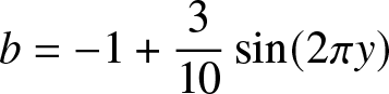 \begin{align}
b & = -1 + \frac{3}{10} \sin(2\pi y)
\end{align}
\begin{align}
b & = -1 + \frac{3}{10} \sin(2\pi y)
\end{align}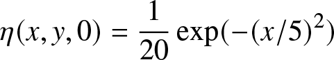 \begin{align}
\eta(x,y,0) & = \frac{1}{20} \exp(-(x/5)^2)
\end{align}
\begin{align}
\eta(x,y,0) & = \frac{1}{20} \exp(-(x/5)^2)
\end{align} \begin{align}
u(x,y,0) & = 0
\end{align}
\begin{align}
u(x,y,0) & = 0
\end{align}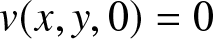 \begin{align}
v(x,y,0) & = 0
\end{align}
\begin{align}
v(x,y,0) & = 0
\end{align}Although the same problem is solved using the PS and FV methods, the computational setup is slightly different.
For the PS code, we take  $(x,y)\in [-1000,1000]\times[-1/2,1/2]$ and impose periodic boundary conditions at all boundaries. The final time is chosen such that the waves do not reach $x=\pm1000$.
For the FV code, we can save computational effort by taking only the right half of the domain:  $(x,y)\in [0,1000]\times[-1/2,1/2]$. Due to the symmetry of the solution, we can impose a reflecting boundary condition at x = 0 and obtain the solution of the same problem, restricted to the right half of the domain. However, this is still quite expensive, so to save even more computational effort we do as follows. We take a much smaller domain ( $(x,y)\in [0,100]\times[-1/2,1/2]$). We impose a reflecting boundary condition at x = 0 initially; once the waves have moved away from the origin we impose periodic boundary conditions in x. This allows us to simulate the right-going wave train with high resolution at a reasonable computational cost. The simulation ends long before the leading wave would begin to catch up to the tail of the wave train. This is possible because the solution is nearly constant far away from the main waves.
Results are shown in Figure 2. The initial surface perturbation splits into a left-going and right-going pulse, each of which eventually resolves into a series of travelling waves. We see a remarkably close agreement between all three solutions, up to t = 200.
Comparison of homogenized and direct solutions, for sinusoidal bathymetry (29a). The surface elevation  $\eta - \eta^0$ is shown.
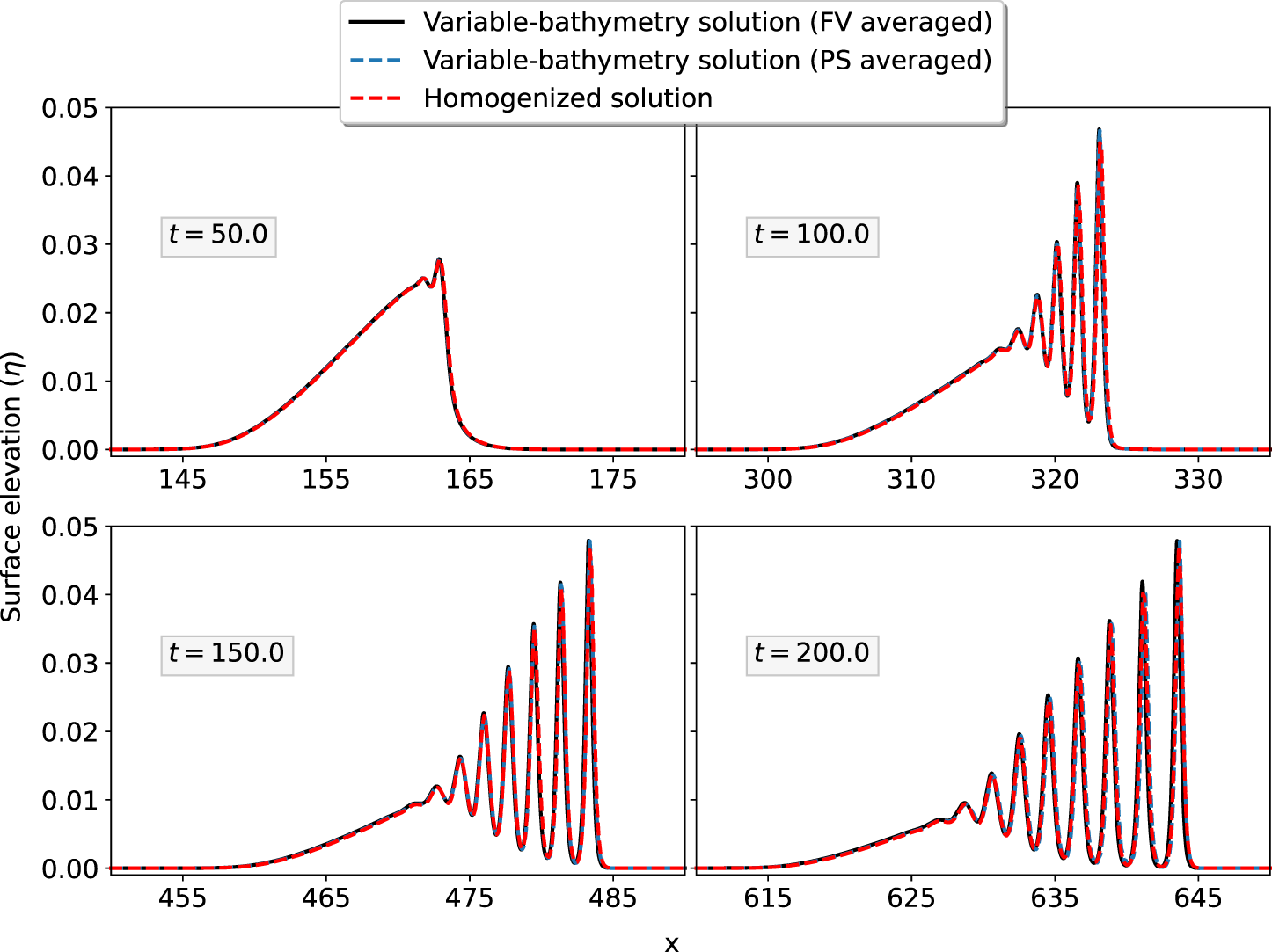
To obtain the results shown here, we used a mesh of  $32,000 \times 32$ points for the 2D PS code and $16,000\times 160$ points for the 2D FV code. For the 1D homogenized equations, the pseudospectral simulation was performed on a grid with 32,000 points.
3.4. Piecewise-constant bathymetry
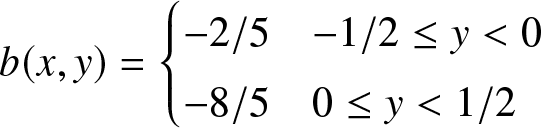
We next consider the discontinuous bathymetry:
 \begin{align}
b(x,y) & = \begin{cases} -2/5 & -1/2 \le y \lt 0 \\ -8/5 & 0 \le y \lt 1/2 \end{cases}
\end{align}
\begin{align}
b(x,y) & = \begin{cases} -2/5 & -1/2 \le y \lt 0 \\ -8/5 & 0 \le y \lt 1/2 \end{cases}
\end{align}with the same initial data as in (29). In this case, we cannot use the 2D PS solver due to the lack of continuity of the solution. For the FV simulation, the domain and boundary conditions are set up in the same way as for the problem above.
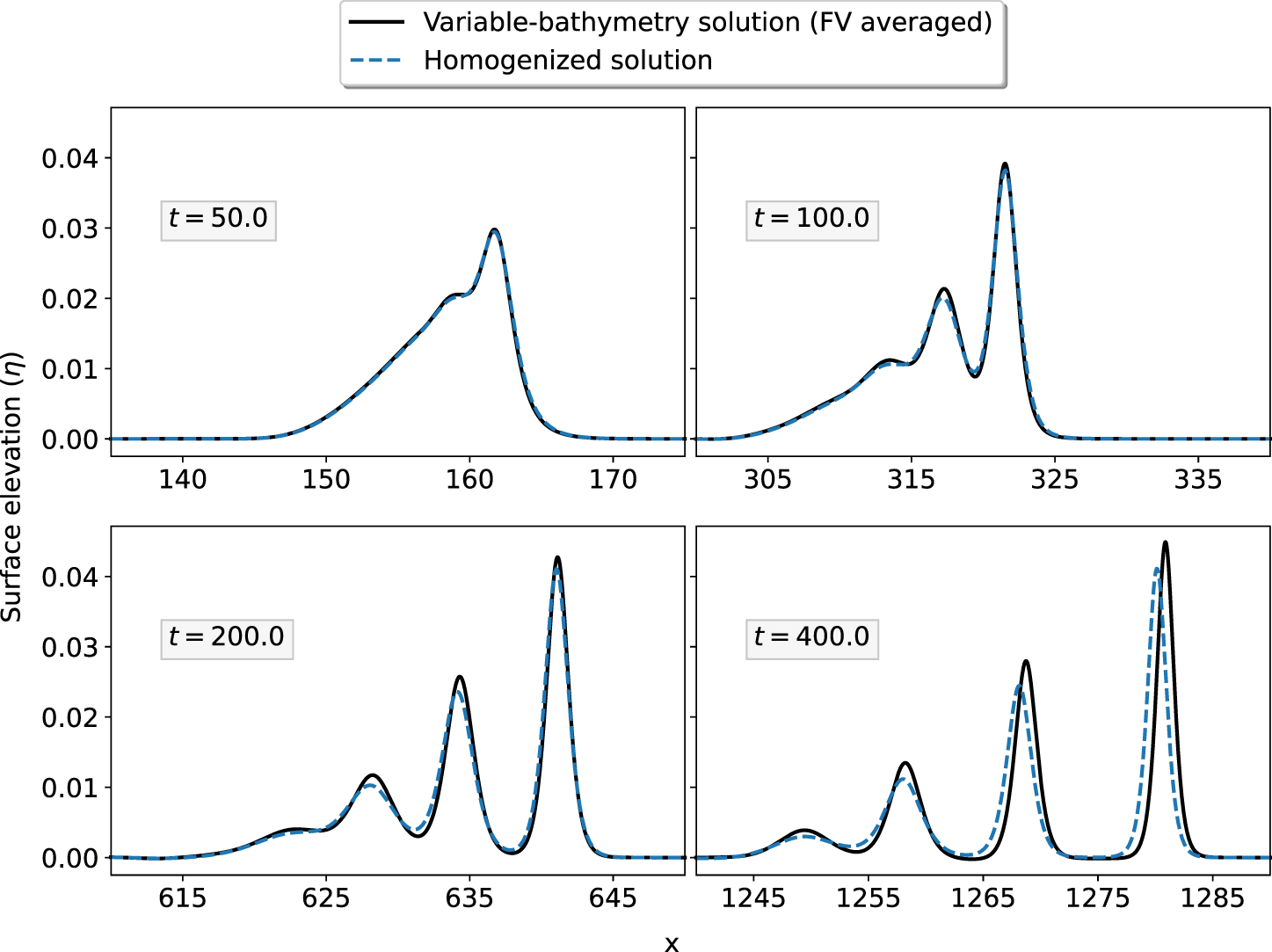
In Figure 3, we show snapshots of the right-going pulse. We see extremely close agreement between the solutions, with some differences visible at late times, after the pulse has propagated for hundreds of meters.
Comparison of homogenized and direct solutions, for piecewise-constant bathymetry (30). The surface elevation  $\eta - \eta^0$ is shown.
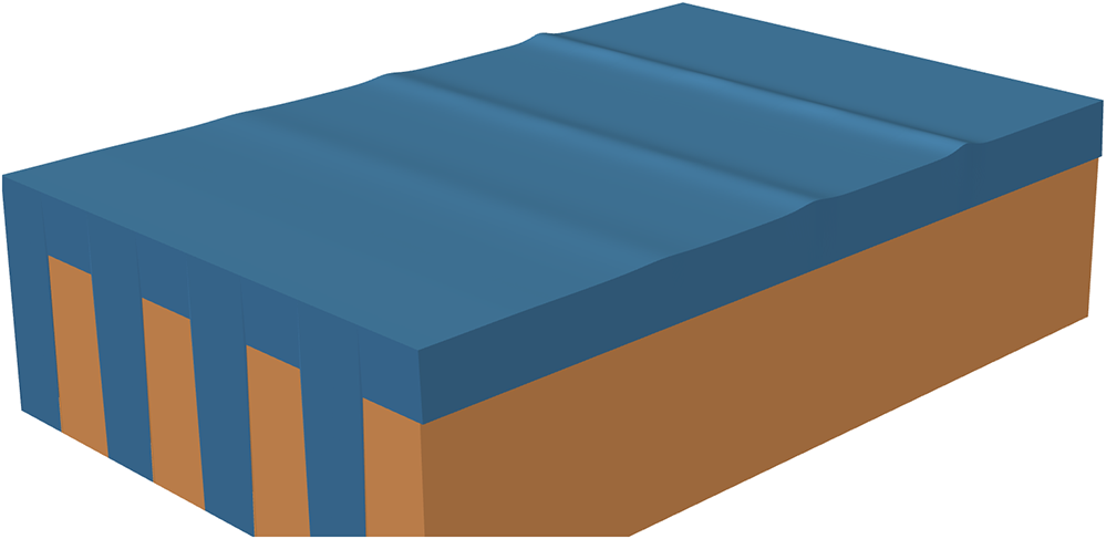
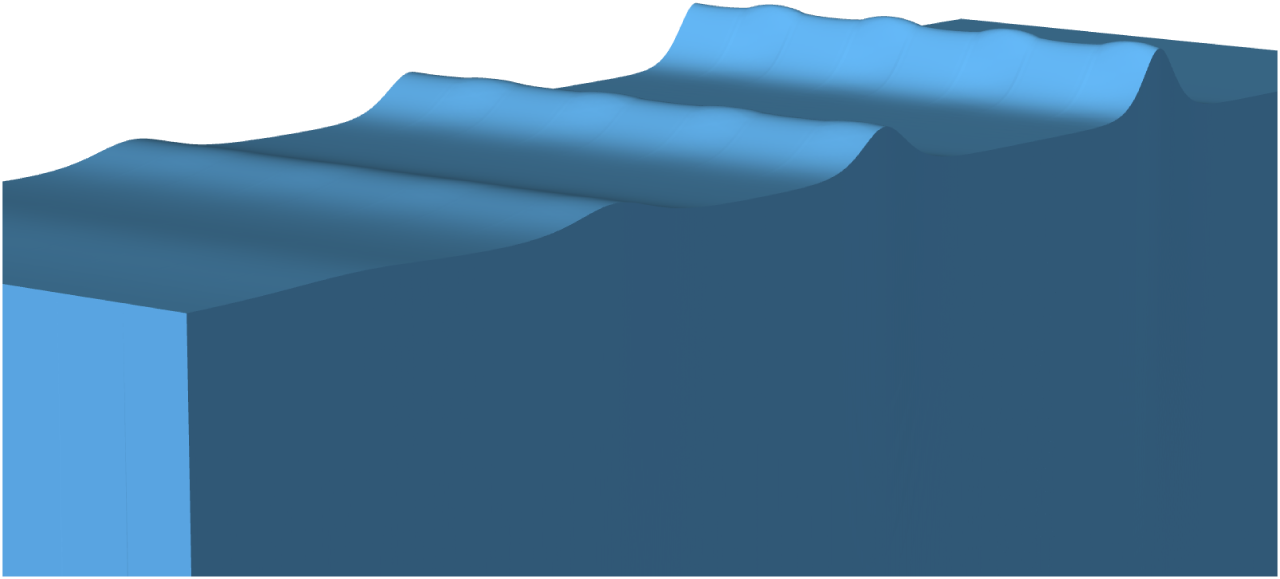
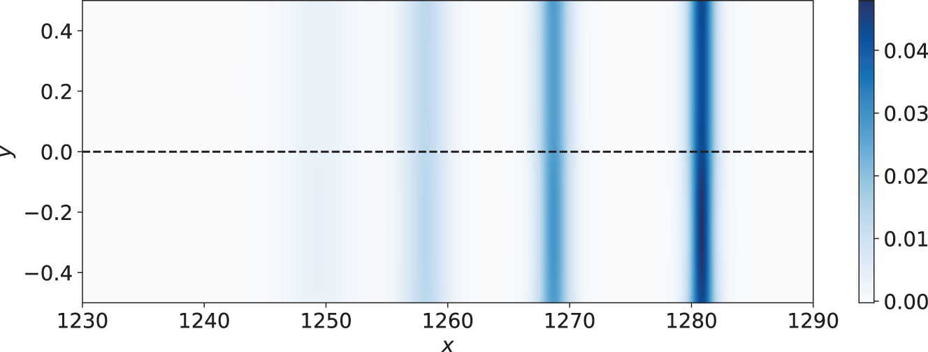
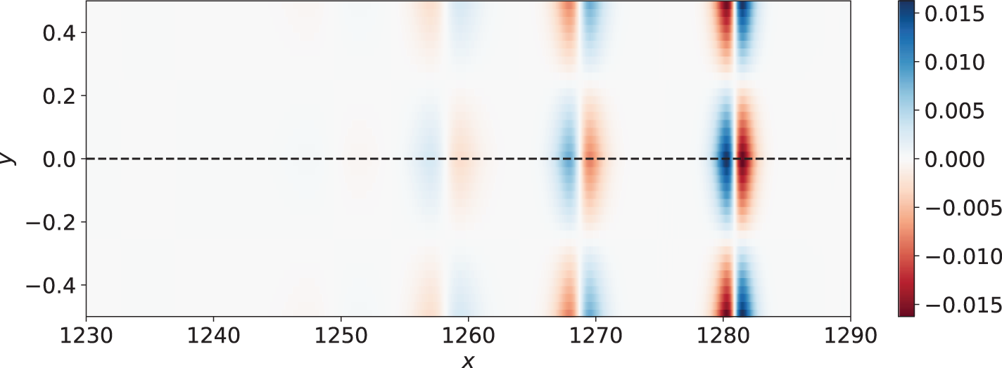
The solution at the final time is also shown in Figures 4–7. Although the characteristic speed varies greatly as a function of y, the surface elevation profiles remain almost perfectly planar. The mechanism for this can be seen in Figure 7, which exhibits a small flow from the deep region to the shallow region at the front of each solitary wave, and a similar flow from the shallow region to the deep region at the back of each solitary wave. One can also view each solitary wave as a superposition of an upward-travelling wave with an oscillatory shape (shown in blue in Figure 7) and a downward-travelling wave with an oscillatory shape (shown in red). These two waves combine to yield highly planar surface and x-velocity fields.
Three-dimensional rendering of the FV solution shown in the last panel of Figure 3. Results shown are to scale, except that the x-axis has been compressed by a factor of 8 to make it easier to see the waves.
Closeup of the surface waves shown in Figure 4. The vertical variation has been exaggerated by 10x and the x-axis has been compressed by a factor of 8 to make it easier to see the waves.
Surface elevation for the FV solution shown in the last panel of Figure 3.
y-momentum for the FV solution shown in the last panel of Figure 3.
As predicted by equation (26), the wave height does vary to a small degree with y; this can be seen in Figure 5. We examine this variation more carefully in Section 4.
4. Solitary wave shape
In this section, we study the shape of the solitary waves observed in numerical simulations and compare them with predictions based on the homogenized equations. We first consider travelling wave solutions of the homogenized equations and then investigate the full two-dimensional solitary waves in more detail.
4.1. Travelling wave solutions of the homogenized equations
Now we consider the problem of finding the travelling wave solution for the homogenized system (23). Neglecting the higher order term, after dividing by δ, and neglecting terms of  ${\mathcal O}{(\delta^3)}$, the system can be written in the form
 \begin{align*}
q_t + a_1 \eta_x + a_2 q q_x - \tilde{\mu}q_{xxt} & = 0
\end{align*}
\begin{align*}
q_t + a_1 \eta_x + a_2 q q_x - \tilde{\mu}q_{xxt} & = 0
\end{align*} \begin{align*}
\eta_t + q_x + a_2(\eta q)_x & = 0
\end{align*}
\begin{align*}
\eta_t + q_x + a_2(\eta q)_x & = 0
\end{align*} where we set  $a_1:=g\langle H \rangle$, $a_2 := \delta/\langle H \rangle$, $\tilde{\mu} := \delta^2\mu/\langle H \rangle$.
This is the classical Boussinesq model with linear dispersion, which has been widely studied in the literature (see, for example, [Reference Chen4]). To be more self-contained, we summarize here the main steps of the procedure.
We look for travelling waves which depend only on  $\xi = x-Vt$, propagating on a lake at rest, so that the unperturbed state is $q_0=0$, and, with a suitable choice of the frame of reference, $\eta_0 = 0$. Here V is the travelling speed of the wave. Assuming η and q are functions of ξ, we obtain that the wave satisfies an equation of the form
 \begin{equation}
q'' = F(q),
\end{equation}
\begin{equation}
q'' = F(q),
\end{equation}with
 \begin{equation*}
\eta = \frac{q}{V-a_2 q}.
\end{equation*}
\begin{equation*}
\eta = \frac{q}{V-a_2 q}.
\end{equation*} Multiplying by  $q'$ and integrating we obtain the analogue of total energy conservation
 \begin{align}
\frac12 (q')^2 + U(q) = E,
\end{align}
\begin{align}
\frac12 (q')^2 + U(q) = E,
\end{align}with
 \begin{equation*}
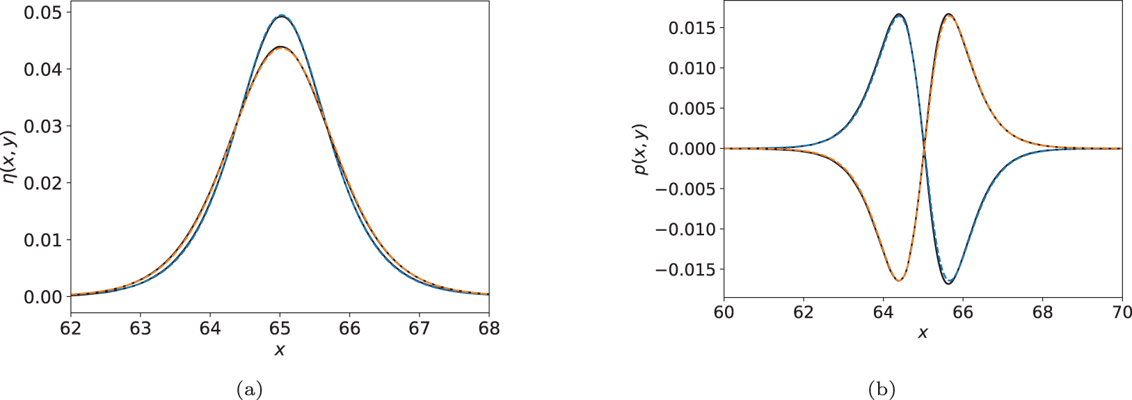
U(q) = \left(\frac16a_2q^3-\frac12Vq^2-\frac{a_1}{a_2}q
-\frac{a_1}{a_2^2}V\log(1-a_2 q/V)\right)/(\tilde{\mu} V).
\end{equation*}
\begin{equation*}
U(q) = \left(\frac16a_2q^3-\frac12Vq^2-\frac{a_1}{a_2}q
-\frac{a_1}{a_2^2}V\log(1-a_2 q/V)\right)/(\tilde{\mu} V).
\end{equation*} The trajectories of the material point in phase space  $(q,\dot{q})$ are the lines that maintain constant total energy. Notice that if we approximate the log term by the first term in its expansion about q = 0, then the solution of (34) is a hyperbolic secant squared. Thus we expect that solitary waves will be close to this shape.
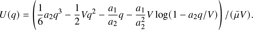
An example of potential, trajectories and travelling waves are illustrated in Figure 8. The first panel shows both the potential U(q) corresponding to  $V = 10/3$ (blue continuous line) and its best fit approximation with a cubic polynomial (magenta dashed line). The middle panel shows the structure of this dynamical system, with two equilibria and a homoclinic connection. The right panel is obtained by integrating (33) written as a pair of first-order equations, along the homoclinic connection, starting from a very small perturbation of the saddle equilibrium state, with the perturbation in the direction of the eigenvector of the linearized dynamical system corresponding to the positive (unstable) eigenvalue.
Construction of the travelling waves. Left panel: potential U(q) corresponding to  $V=10/3$ (blue continuous line). If total energy is low enough and the particle is initially in the potential well, then the orbits are periodic (black line between points A and B). As the energy increases approaching zero from below, the period of the oscillations tends to infinity, and the trajectory becomes a travelling wave. Positive energy corresponds to open orbits. The middle panel shows the lines with constant total energy corresponding to the same potential. The thick red line is the separatrix. The right panel is obtained by numerically integrating (33) along the separatrix trajectory.
4.2. Mean profile
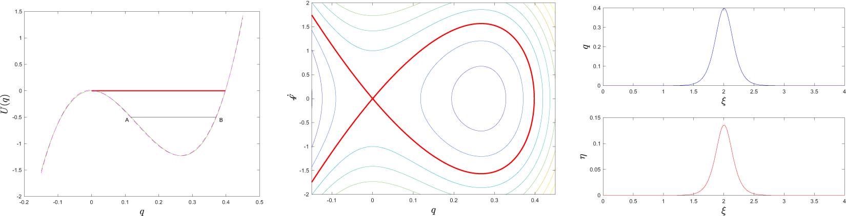
First we consider the shape of the y-averaged surface. A typical y-averaged solution is shown in Figure 9(a). As expected, these waves have a shape very close to the typical  $\operatorname{sech}^2$ and seem to scale in the same way as other such solitons. In Figure 9(b), we plot each of the three tallest waves, after shifting the peak to be at x = 0, rescaling the amplitude to 1 and rescaling the width by the square root of the amplitude. We see that the waves very nearly coincide with the reference $\operatorname{sech}^2$ curve. This is not surprising, given that the potential in the first panel of Figure 8 is very well approximated by a cubic polynomial.
The mean surface height for small-amplitude solitary waves (solid lines) is very close to  $\operatorname{sech}^2$ (dashed line), and the waves’ width scales inversely with the square root of the amplitude. a) Mean surface height versus x for a train of solitary waves. b) Largest 3 waves rescaled and compared with a fitted $\operatorname{sech}^2$ curve.
We have observed that much larger solitary waves have a more sharply peaked shape; investigation of larger-amplitude solutions is the subject of ongoing work.
4.3. Full shape
Our travelling wave analysis shows that small-amplitude solitary wave solutions have the y-averaged surface profile
 \begin{align}
\langle \eta \rangle(x,t) \approx A \operatorname{sech}^2(\alpha\sqrt{A}(x-Vt),
\end{align}
\begin{align}
\langle \eta \rangle(x,t) \approx A \operatorname{sech}^2(\alpha\sqrt{A}(x-Vt),
\end{align}where A is the wave amplitude, V is the velocity and α is related to the width; for the present scenario α ≈ 4.85. The full approximate shape of these waves is then predicted by the formulas in Section 2.6. In particular, for a fixed time t we have (up to translation)
 \begin{align}
\eta(x,y,t) \approx A \operatorname{sech}^2(\alpha\sqrt{A}x) - \delta^2 \unicode{x27E6} H^{-1}\unicode{x27E6} H \unicode{x27E7} \unicode{x27E7} \frac{d^2}{dx^2}\left(A\operatorname{sech}^2(\alpha\sqrt{A}x)\right).
\end{align}
\begin{align}
\eta(x,y,t) \approx A \operatorname{sech}^2(\alpha\sqrt{A}x) - \delta^2 \unicode{x27E6} H^{-1}\unicode{x27E6} H \unicode{x27E7} \unicode{x27E7} \frac{d^2}{dx^2}\left(A\operatorname{sech}^2(\alpha\sqrt{A}x)\right).
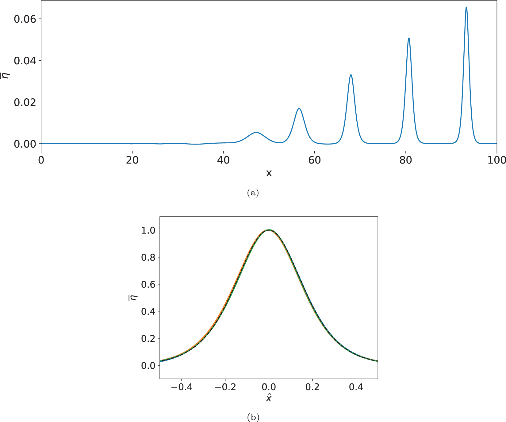
\end{align}In Figures 10 and 11, we plot a numerical solitary wave versus the formulas from Section 2.6, as a function of x for two slices in y, and as a function of y for slices in x. Note that here, to fit the full two-dimensional solitary wave, we have used only the mean peak amplitude as a fitting parameter. Thus the waves we observe seem to belong to a one-parameter family.
Comparison of solitary wave shape (computed via FV) with the formulas obtained from homogenization. FV solutions are shown as solid black lines and predictions from homogenization are shown as coloured dashed lines. a) Computed FV surface height (in black) versus x compared to (36), for  $y=-19/80$ (dashed blue line) and $y=19/80$ (dashed orange line). b) Computed FV y-momentum (p, in black) versus x compared to (24), for $y=-1/80$ (dashed blue line) and $y=39/80$ (dashed orange line).
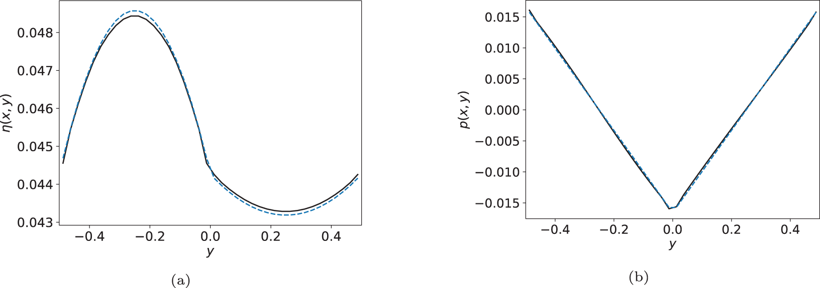
Comparison of solitary wave shape (computed via FV) with the formulas obtained from homogenization, as function of y. FV solutions are shown as solid black lines and predictions from homogenization are shown as coloured dashed lines. At the peak of the wave, p vanishes, so the plot of p is taken at a point away from the wave peak. a) Computed FV surface height (in black) versus y compared to (36) (dashed blue line), for x = 65.1375 . b) Computed FV y-momentum (p) (in black) versus y compared to (24), for x = 65.4875 (dashed blue line).
Similar investigation of solitary waves over other bathymetric profiles (including smooth sinusoidal bathymetry) show that the waves have, to very good approximation, the shape prescribed in Section 2.6.
5. Conclusion
We have studied the behaviour of initially planar shallow water waves over a bottom that varies periodically in the transverse direction. These waves are described to good accuracy by the effective Boussinesq system (23) and exhibit the formation of solitary waves. Unlike solitary wave solutions of one-dimensional hyperbolic systems with periodic coefficients [Reference Ketcheson, Lóczi and Russo6, Reference LeVeque and Yong9], these are true travelling waves. The shape of small-amplitude solitary waves is close to one that can be expressed simply in terms of elementary functions and is predicted by the equations obtained in the process of deriving the effective Boussinesq system. The assumption of a small amplitude wave is natural since sufficiently large-amplitude waves will exhibit shocks. Nevertheless, in numerical experiments, we have successfully produced approximate travelling wave solutions that are 2-3 times larger than those shown in this work.
Since water waves are naturally dispersive (even over a flat bottom), it is natural to ask about the behaviour of water waves over periodic bathymetry when both natural dispersion and bathymetric dispersion are accounted for. This has been studied to some extent in [Reference Chassagne, Filippini, Ricchiuto and Bonneton3, Reference Quezada de Luna and Ketcheson13]; a full analysis starting from a dispersive water wave model is the subject of future work and seems to require techniques beyond what we have used herein.
Many other questions about the behaviour of these waves remain open. For instance, large-amplitude solitary waves have a different shape, and sufficiently large initial data lead to wave breaking, but the behaviour of waves near the boundary between the dispersion-dominated and nonlinearity-dominated regime is complicated. The interaction of colliding solitary waves and the behaviour of periodic travelling waves in this system are also of interest.
Acknowledgements
This work was supported by funding from King Abdullah University of Science and Technology (KAUST). It was carried out in large part while the second author was a visiting professor at KAUST. G. Russo would like to thank the Italian Ministry of University and Research (MUR) to support this research with funds coming from PRIN Project 2022 (No. 2022KA3JBA) entitled “Advanced numerical methods for time-dependent parametric partial differential equations with applications”.
Competing Interests
The authors have no competing interests.


 Open access