


Impact Statement
Gap resonance may occur at certain frequencies, for offshore operations where two bodies are parked in close proximity, e.g. liquefied natural gas offloading, ship-to-ship transfers. The current practice to predict the most probable extreme responses has been to rely on time-domain simulations, which are time consuming and usually validated against scaled model tests. However, the flow field at full scale could be different. This study proposes an efficient model, identifying the design waves that induce the most probable maximum responses. This enables quick identification of the lower and upper bounds of the statistics along the gap, which is crucial for decision making at sea. The method has been adopted to gap resonance between two fixed bodies, it is expected that it will be applicable to floating bodies and other offshore facilities. This study could be of particular value for design of offshore renewable energy devices, reducing their cost through an efficient prediction model.
1. Introduction
Gap resonance is a wave–structure interaction phenomenon, where the potential flow damping is small due to the difficulty for waves ‘escaping’ from the gap and thus the viscous damping becomes important. An obvious application scenario is the offloading operation of liquefied natural gas (LNG) at sea, where an LNG carrier is parked alongside a floating LNG facility in close proximity, forming a narrow (relative to its length) gap.
Recent developments on gap resonance have been reported in our previous study (Reference Zhao, Wolgamot, Taylor and Eatock TaylorZhao, Wolgamot, Taylor, & Eatock Taylor, 2017), and thus we only provide a summary here. The frequencies of the gap resonance modes can be well predicted by analytical formula (e.g. Reference MolinMolin, 2001) and numerical simulations (e.g. Reference ChenChen, 2005; Reference NewmanNewman, 2001), based on linear potential flow theory. However, predicting the response amplitudes requires estimation of the viscous damping. Various methods have been adopted to incorporate the viscous damping contribution, such as those reported in Reference ChenChen (Reference Chen2005) for three-dimensional (3-D) and Reference Faltinsen and TimokhaFaltinsen and Timokha (Reference Faltinsen and Timokha2015) for two-dimensional (2-D) cases. All the various numerical results seem to match well the experimental data, with an appropriate coefficient – representing the viscous damping – being chosen. Therefore, it is important to understand the nature of the viscous damping, and this has been studied, e.g. Reference Tan, Lu, Tang, Cheng and ChenTan, Lu, Tang, Cheng, & Chen (Reference Tan, Lu, Tang, Cheng and Chen2015).
It is worth emphasising that the gap resonant modes in a 3-D scenario are more complicated than those in a simplified 2-D gap. For instance, only the piston mode can be observed in a simplified 2-D gap (e.g. Reference Jiang, Bai and TangJiang, Bai, & Tang, 2019), while a series of gap modes – each being an integer number of half-wavelengths along the gap – can be excited in a 3-D gap (e.g. Reference Molin, Zhang, Huang and RemyMolin, Zhang, Huang, & Remy, 2018). The resonant response in the former situation is much stronger, as there is no gap end for waves to ‘escape’ from.
To examine the temporal (Reference Zhao, Wolgamot, Taylor and Eatock TaylorZhao et al., 2017) and spatial structure (Reference Zhao, Taylor, Wolgamot, Molin and Eatock TaylorZhao, Taylor, Wolgamot, Molin, & Eatock Taylor, 2020) along the gap, we conducted a series of experiments for two fixed vessel models in side-by-side configuration. It is found in Reference Zhao, Wolgamot, Taylor and Eatock TaylorZhao et al. (Reference Zhao, Wolgamot, Taylor and Eatock Taylor2017) that the viscous damping inside the gap behaves in a linear form at the large laboratory scale. This is because the oscillatory boundary layer in our large scale  $(1 : 60)$ tests is in the ‘disturbed’ laminar boundary layer, as discussed in Reference Blondeaux and VittoriBlondeaux and Vittori (Reference Blondeaux and Vittori2021). For instance, according to the definition of Blondeux $\&$ Vittori, the maximum Reynolds number in our experiment is $R_{\delta }=u\sqrt {2/{(\omega {v})}}\approx 180$, where $u$,
$u$,  $\omega$ and $v$ denote the velocity amplitude, oscillatory frequency and kinematic viscosity of the fluid, respectively. It remains unclear how the damping will behave at full scale. Further discussion on scaling from the laboratory scale to the field is given in § 5.1. Ultimately, it is of practical interest to understand the response statistics along the gap, to facilitate decision making for offshore operations.
In contrast to our previous studies (Reference Zhao, Taylor, Wolgamot, Molin and Eatock TaylorZhao et al., Reference Zhao, Taylor, Wolgamot, Molin and Eatock Taylor2020, Reference Zhao, Wolgamot, Taylor and Eatock Taylor2017) which unravelled new physics, this study focuses on a totally different aspect – the most probable extreme gap response in a random sea that is of great interest to engineering practice. Here we identify the design waves (localised wave groups) that produce the most probable maximum (MPM) responses under linear wave excitations. This study is organised as follows. Following this introduction, the experimental set-up in a wave basin is described in § 2. The theoretical background is presented in § 3, including the NewWave-type analysis and the design waves. The predicted MPM responses and the corresponding design waves are given in § 4 for different locations along the gap. The variation of the statistics along the gap are discussed in § 5 for different heading conditions. Finally, § 6 presents some conclusions.
2. Experiments
2.1. Experimental set-up
The experiments were conducted in the Deepwater Wave Basin at Shanghai Jiao Tong University. The basin is 50 m long, 40 m wide and the water depth was set to 10 m. To focus on the gap resonances and simplify the study, we selected two identical rectangular boxes to represent a side-by-side moored two-body system. Each model is 3.333 m long, 0.425 m high, 0.767 m wide and the gap width between them is 0.067 m. The vessel models have round corners at both bilges, each with a radius of 0.083 m running along the full length, as shown in figure 1.
Experimental set-up: (a) sketch (not to scale) of the fixed boxes in different heading excitations, with the red cross symbols showing the locations of the wave probes; (b) a snapshot of the fixed box hull (yellow) rigidly connected to the gantry (blue) in the wave basin. This figure is similar to that in Reference Zhao, Taylor, Wolgamot, Molin and Eatock TaylorZhao et al. (Reference Zhao, Taylor, Wolgamot, Molin and Eatock Taylor2020), but shown here to facilitate reading.

Each box was immersed to a draft of 0.185 m and rigidly fixed to the stiff bridge across the basin, as shown in figure 1. There are seven wave gauges (WG) 1 and 7, 2 and 6, 3 and 5 being symmetric in pairs about the gap centre, and WG4 being central in the gap. Wave gauges 0 and 8 are deployed right at the two ends of the gap. Further details on the experimental set-up were reported in our previous studies (Reference Zhao, Taylor, Wolgamot, Molin and Eatock TaylorZhao et al., 2020, Reference Zhao, Wolgamot, Taylor and Eatock Taylor2017). In this study, we investigate the statistical structure along the gap.
We used transient focused wave groups as the incident waves, to avoid contamination by the reflections from the basin walls or the far end of the basin. To calibrate the undisturbed incident waves, a series of transient wave groups were generated in the absence of the model, based on a hypothetical Gaussian spectrum given by
 \begin{equation} S_\eta(f) = \frac{H_s^2}{16}\frac{1}{\delta\sqrt{2{\rm \pi}}} \exp\left[-\frac{(f-f_p)^2}{2{\delta}^2}\right],\end{equation}
where  $H_s$ refers to an assumed significant wave height, $f_p$ the peak frequency of the spectrum and $\delta=0.0775$ s $^{-1}$. The fixed models are rotated to achieve different wave approach directions. All the data in this study have been sampled at a frequency of 25 s $^{-1}$.
2.2. Linear transfer functions
Transient wave groups (see § 3) were generated, with a spectral peak frequency  $f_p=f_{m=1}=1.02$ s $^{-1}$, where $f_{m=1}$ is the frequency of the mode with one half-wavelength along the gap in this experiment. The gap modes can be split into two types: one type is symmetric with respect to the midship, the other is antisymmetric. A detailed description of the mode shapes can been found in our previous study (Reference Zhao, Taylor, Wolgamot, Molin and Eatock TaylorZhao et al., 2020).
The target maximum surface elevation for the crest-focussed incident wave packet for these experiments in the laboratory was 50 mm. The focus position, which was also the location of the centre of the gap, was set at  $x_0=19.83$ m from the equilibrium position of the wave paddles. The wave spectrum was divided into 500 wave components in the frequency range 0.25 s $^{-1}$ to 2.50 s $^{-1}$. The wave paddle signals which generated these wave groups were stored and repeated with the model in place producing the data analysed in the following sections.
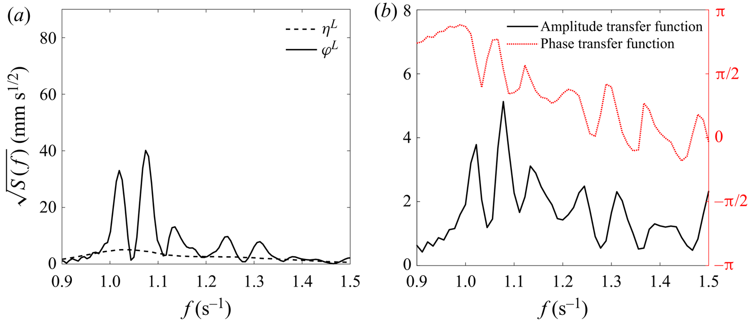
After collecting the measurement data, we extract the harmonic components based on the four-phase decomposition method as demonstrated in Reference Zhao, Wolgamot, Taylor and Eatock TaylorZhao et al. (Reference Zhao, Wolgamot, Taylor and Eatock Taylor2017). Rather than repeating the time histories here, we show the results in the frequency domain, which facilitates the demonstration of the linear transfer functions. Figure 2 shows the results at the centre of the gap in beam sea excitation. The linear transfer function ( $LTF$), shown in figure 2(b), is obtained by simply calculating the ratio of the Fourier components of the gap responses ( $\varphi$) and the undisturbed incident wave ( $\eta$), i.e. $LTF=FFT(\varphi ^L)/FFT(\eta ^L)$, where the superscript ‘ $L$’ refers to the linear component. We only show the frequency range 0.9 s $^{-1}$ to 1.5 s $^{-1}$, where the gap mode resonances are important (shown as the multiple peaks). There is no gap mode at frequencies less than 0.9 s $^{-1}$, while at frequencies higher than 1.5 s $^{-1}$ the gap mode resonances are weak and thus less important, at least for the experimental case studied here. As a result, the undisturbed incident wave is designed to concentrate incident wave energy from 0.9 s $^{-1}$ to 1.5 s $^{-1}$.
Spectra and linear transfer function of the water surface elevations at the centre of the gap with and without the model in place, in beam sea excitation: (a) response spectra for undisturbed incident waves  $\eta ^{L}$ and the resulting gap resonance $\varphi ^{L}$; (b) amplitude and phase of the linear transfer function. The superscript ‘ $L$’ refers to the linear component. The frequency resolution for the transfer function is 0.011 s $^{-1}$ which is determined by the limited duration (90 s) of the wave group.

To compare with the beam sea condition, figure 3 shows the gap resonance results in the head sea excitation. It is noted that the centre of the gap, where WG4 is located, is a node for the even gap modes. Therefore, rather than using results at WG4, we show the results measured at WG2 in figure 3. Figure 3 clearly shows more peaks compared with those in figure 2, this is simply because both odd and even modes along the gap are excited in the head sea excitation, where the symmetry of the excitation is broken.
Same as in figure 2, but measured at WG2 in head sea excitation.
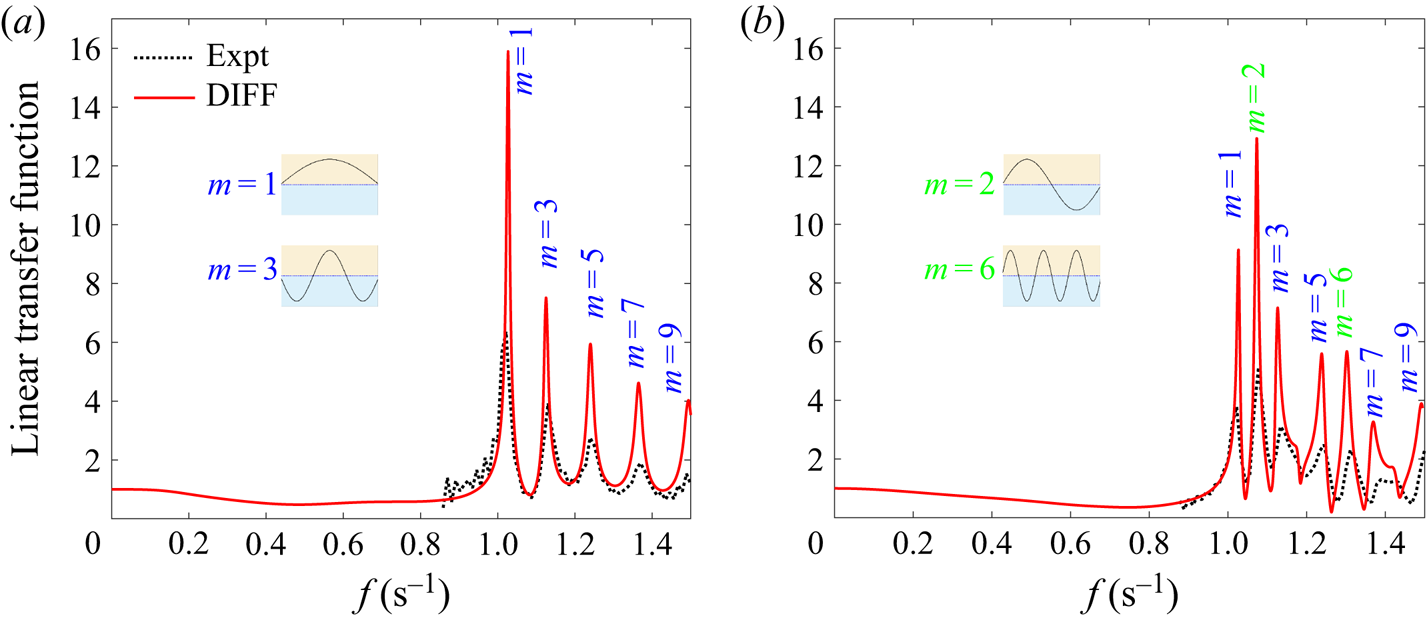
It is understood that the experimental results cover both radiation damping and viscous damping, limiting the gap resonance amplitudes; while linear potential flow calculations, where viscous damping is ignored which otherwise needs to be identified by experiments, produce much larger resonant responses. To demonstrate the significant difference, we run the potential flow code DIFFRACT as in Reference Zhao, Wolgamot, Taylor and Eatock TaylorZhao et al. (Reference Zhao, Wolgamot, Taylor and Eatock Taylor2017), where more details have been given. Figure 4 compares the experimentally determined linear transfer functions with those obtained through linear potential flow calculations (without any viscous damping). It is not surprising that the viscous damping plays a significant role – reducing response amplitude – at resonances, while it is less important off the resonant frequencies. This is supported by the fact that in the frequency range between 0.85 s $^{-1}$ to 1.00 s $^{-1}$ (off resonance), the numerical simulations match the experimental data. It is then sensible to use the linear potential flow calculations to show more response information towards zero frequency, which is of academic interest.
Modulus of the linear transfer functions, (a) for beam sea at WG4 (centre of the gap) and (b) for head sea at WG2. The dotted lines are experimentally determined as in figures 2 and 3, and the red curves are obtained based on the potential flow code DIFFRACT (see details in Reference Zhao, Wolgamot, Taylor and Eatock TaylorZhao et al. (Reference Zhao, Wolgamot, Taylor and Eatock Taylor2017)). Representative resonant mode shapes are demonstrated to facilitate reading. Note WG2 is a node for the  $m=4$ mode and thus has no corresponding response peak in panel (b).
In addition to WG2 and WG4, linear transfer functions are also obtained for other locations along the gap, but not shown here for the sake of simplicity. The linear transfer functions are then adopted to estimate the most probable extreme responses in random seas using a time-efficient analysis model as demonstrated in § 3.
3. Theory associated with NewWave analysis
Focused transient wave groups are adopted to excite the gap resonance in this study. These are generated adopting the NewWave theory (Jonathan & Taylor, Reference Jonathan and Taylor1997; Tromans, Anaturk, & Hagemeijer, Reference Tromans, Anaturk and Hagemeijer1991), which is based on the theory by Lindgren (Reference Lindgren1970) and Boccotti (Reference Boccotti1983). In the NewWave theory, the wave surface profile (in time) at the focus point is given by
 \begin{equation} \eta^{{N}} = \frac{\alpha_\eta}{\sigma_\eta^2} \sum_{n = 1}^N{S_\eta(f_n)}{\Delta}f{{Re}} [\mathrm{e}^{\textrm{{i}}2{\rm \pi}f_nt}],\end{equation}
where  $k_n$ and $f_n$ are the wavenumber and frequency of the spectral components and the variance $\sigma _\eta ^2=\sum _{n=1}^N{S_\eta (f_n)}{\Delta }f$.
This NewWave profile ( $\eta ^{{N}}$) is the most probable shape in time of an extreme crest event in a linear random Gaussian sea state. One can see that the structure of $\eta ^{{N}}$ is defined by the shape of the energy spectrum $S_\eta (f_n)$. The MPM free-surface elevation $\alpha _{\eta }$ corresponds to the linear magnitude of the NewWave crest, which is set by the 1 in $N$ largest linear crests in a random sea state from the Rayleigh distribution, as derived below (Newman, Reference Newman1993). The normalised probability density function for the wave amplitude in a narrow-banded sea state is given as
 \begin{equation} P(\zeta) = \zeta{\mathrm{e}^{-\zeta^2/2}},\end{equation}
where  $\zeta =\alpha _{\eta }/\sigma _{\eta }$ is the normalised amplitude. From the Rayleigh distribution, the cumulative probability of a single wave being less than $\alpha _{\eta }$ is
 \begin{equation} P(\zeta) = \int_{0}^{\zeta}P(\zeta')\, \textrm{d} {\zeta'} = 1-\mathrm{e}^{-\zeta^2/2}. \end{equation}
The peak of the probability density function, which is the most probable extreme wave in  $N$ samples, can be approximated as
 \begin{equation} \alpha_{\eta} = \sqrt{2\sigma_{\eta}^2\log(N)}.\end{equation}
One can see that the MPM  $\alpha _{\eta }$ defines the amplitude of the NewWave. It covers contributions from all the frequency components and varies with the number ( $N$) of waves in the sea state. One can use the zero-crossing period ( $T$) to define the approximate number of waves, e.g. $N=t/T$ where $t$ is the time duration, in a given sea-state duration. The extreme value is not sensitive to how one selects the number $N$, due to the square root of the logarithm $N$.
$N$.
By analogy, the equivalent MPM response in time is defined as NewResponse:
 \begin{equation} \varphi^{{N}} = \frac{\alpha_\varphi}{\sigma_\varphi^2} \sum_{n = 1}^N{S_\varphi(f_n)}{\Delta}f{{Re}} [\mathrm{e}^{\textrm{{i}}2{\rm \pi}f_nt}],\end{equation}
where the variance  $\sigma _\varphi ^2=\sum _{n=1}^N{S_\varphi (f_n)}{\Delta }f$. At any point the surface response ( $\varphi$) with the model in place is related to the incoming waves ( $\eta$) by the linear transfer function. Hence the wave and response spectra are related by $S_{\varphi }(f_n)=S_{\eta }(f_n)|{H(f_n)}|^2$, where $S_{\varphi }$ and $S_{\eta }$ are the power spectra and $H(f_n)$ is the linear transfer function from wave to response.
The NewWave and NewResponse profiles can be obtained from random sea-state excitations, and work well for the gap resonances – highly resonant responses of multiple modes. This has been demonstrated in figures 4 and 5 in our previous study (Reference Zhao, Taylor, Wolgamot and Eatock TaylorZhao, Taylor, Wolgamot, & Eatock Taylor, 2018), and thus we do not repeat them here.
We can also define a wave group – the design wave – which produces a transient response with both the time history and peak value of the MPM response in the random sea state, NewResponse. This design wave is obtained by dividing the response spectrum by the linear transfer function inside the convolution integral (here a sum), as follows:
 \begin{equation} \eta(x,t)|\varphi^{{N}} = \frac{\alpha_\varphi}{\sigma_\varphi^2} \sum_{n = 1}^N{S_\varphi(f_n)}{\Delta}f\cdot{H({f_n})^{{-}1}} \cdot{{Re}}[\mathrm{e}^{-\textrm{{i}}k_nx + \textrm{{i}}2{\rm \pi}f_nt}].\end{equation}
The exponential  $\mathrm {e}^{(-\textrm {{i}}k_nx)}$ is now included as we can ask what the shape of the design wave is anywhere, so away from the point where the extreme response is defined. We stress that the design wave is an incident wave group undisturbed by the presence of the structure which will give the MPM response at the structure and its variation in time.
It is worth emphasising that  $H(f_n)$ presents the ratio between responses and the incident waves at each frequency component, while $\alpha _{\varphi }/\alpha _{\eta }$ is the ratio of the MPM between responses and the incident waves. So the latter is actually a linear transfer function between responses and the incident waves covering contributions from all the frequency components.
As one can see from the discussion above, it is straightforward to obtain the statistics of the responses, as long as we know the linear transfer function and the undisturbed incident waves. For instance, one can obtain the NewResponse based on (6) and the design wave based on (7).
4. Design wave for the most probable extremes
From the design point of view, it is important to identify the most probable extremes of the gap resonances and a ‘design wave’ which produces the extreme responses in a given sea state. The current engineering practice is able to explore the former one based on a Gaussian process, but not for the latter. To obtain both the most probable extremes and the corresponding ‘design wave’ we conduct a NewWave-type analysis as discussed in § 3.
The basic idea is to represent the 1 in  $N$ extreme of a narrow-banded random sea state as a focused transient wave group whose shape is defined by all the frequency components of the wave spectrum and whose amplitude is determined by the combination of the variance and the number of the waves. Here we only consider the linear excitation of the gap, where the linear transfer function obtained in § 2.2 is used.
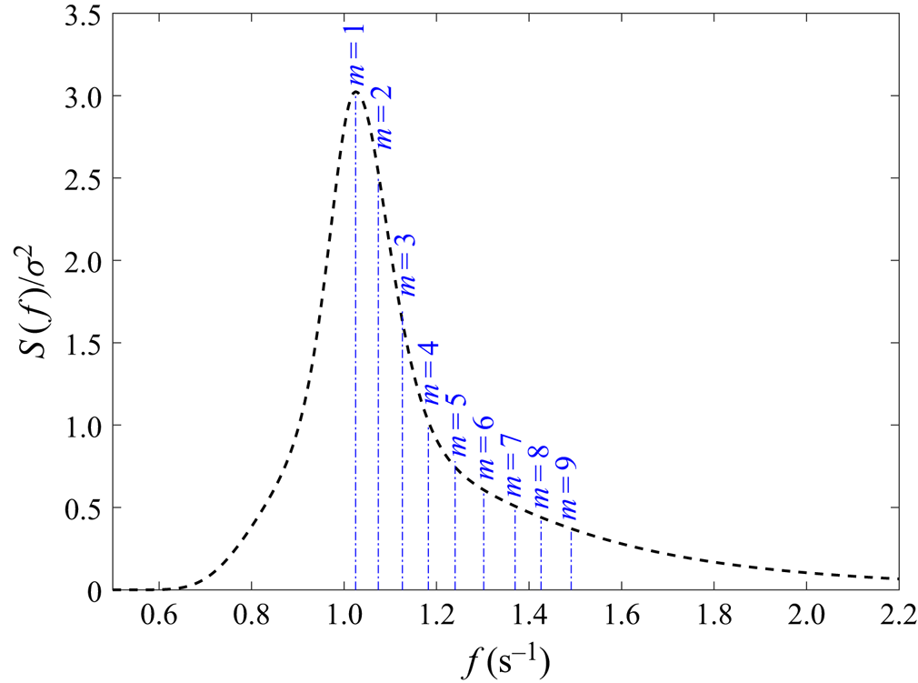
To facilitate the analysis, we assume we have a Joint North Sea Wave Project (JONSWAP) sea state with a wave spectrum with spectral peak  $f_p=f_{m=1}$ (1.02 s $^{-1}$ at laboratory scale) and shape factor $\gamma = 3.3$. The significant wave height does not need to be specified, as we present normalised values in this section and the analysis assumes a linear behaviour. We stress that we are looking at extremes in benign seas, such as Southern Ocean swell, which is close to unidirectional. Therefore, we use unidirectional waves in this study. Figure 5 shows the normalised incident wave spectrum and the frequencies of the first nine gap modes. It would be straightforward to explore the effects of changing the input wave spectral peak frequency relative to the gap mode resonant frequencies, but we have not done this here to save space.
Incident wave spectrum (normalised by its variance). The vertical dash–dotted lines indicate the frequencies of the first nine gap modes.
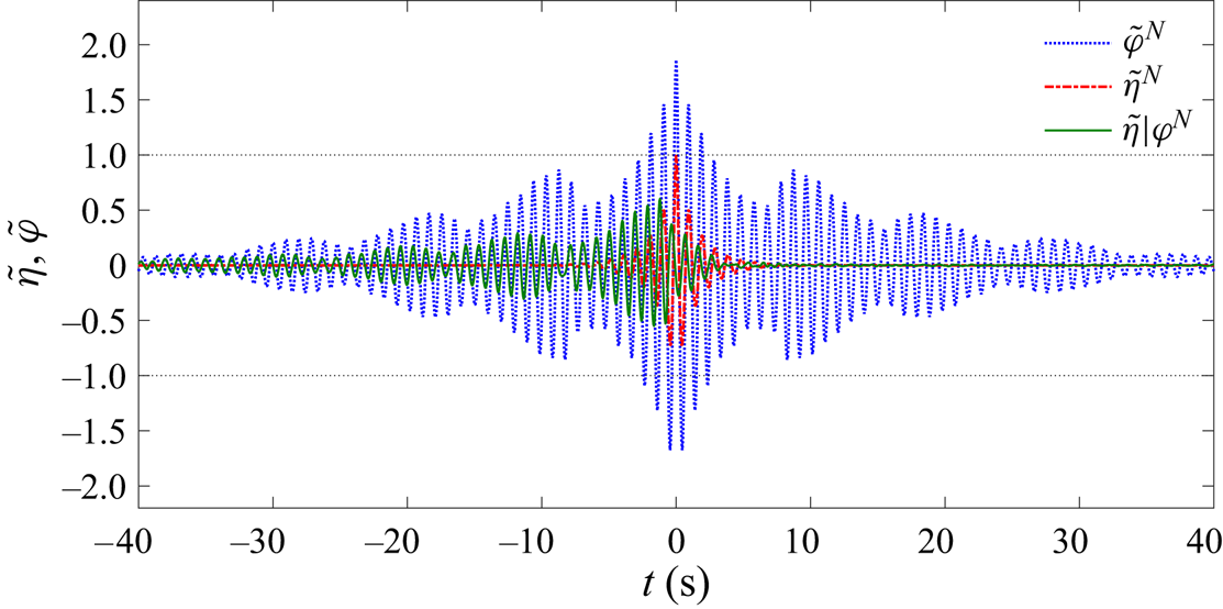
Based on (2) in § 3, a NewWave-type incident wave is generated and normalised by its MPM  $\alpha _{\eta }$, as shown in figure 6 (red dash–dotted curve). The NewWave-type gap response (NewResponse) excited by the same random sea is obtained using (6) (blue dotted curve). The localised wave group – design wave (green solid curve) – which produces the NewResponse in time is obtained based on (7) and again normalised by $\alpha _{\eta }$. One can see that it takes a long time for the design wave to drive the largest gap resonance. The design wave shows a strong beating pattern, which is quite different from, for example, the design wave for the M4 wave power machine discussed in Reference Santo, Taylor, Moreno, Stansby, Eatock Taylor, Sun and ZangSanto et al. (Reference Santo, Taylor, Moreno, Stansby, Eatock Taylor, Sun and Zang2017). The beating pattern here is associated with the superposition of all the different gap resonant modes, whereas the M4 wave energy converter has a single broader but lower resonant peak so the associated decay wave is a simple exponentially decaying sinusoid.
Time histories at WG4 under beam sea excitation: NewResponse ( $\tilde {\varphi }^{{N}}$), the design wave ( $\tilde {\eta }|\varphi ^{{N}}$) that produces this NewResponse and the NewWave ( $\tilde {\eta }^{{N}}$) with the JONSWAP spectrum. The wave hat symbol ‘ $\sim$’ indicates that the time histories have been normalised by the MPM ( $\alpha _{\eta }$) of the incident wave. The frequency resolution of 0.011 s $^{-1}$ is used when calculating these time histories.

Both NewWave and NewResponse are symmetric in time. The response shows the long-term effects of the weakly damped gap modes. Before the maximum, for  $t<0$, energy is pumped into the gap resonant modes but there is also some damping. After the maximum, for $t>0$, the modes simply interfere and slowly decay. In contrast, the design wave is strongly asymmetric: it provides the energy for the modes for $t<0$, thereafter it rapidly disappears, the responses have been driven, thereafter no more input energy is required. It is interesting to note that the time scales involved are so long that no basin anywhere is large enough to do entirely free-field gap resonance experiments (at comparable scale) without some contamination from wall/end effects. Figure 7 shows equivalent results to those in figure 6, but for head sea excitation. The NewResponse and design wave at the centre of the gap in head sea show very similar shape to those in the beam sea excitation, though some differences are visible in the group structure. The similarity is due to the fact that the centre of the gap (WG4) is a node for the even modes, though they have been excited in the head sea excitation. The difference can be explained by the slightly different linear transfer functions at different headings (see figures 4 and 5 in Reference Zhao, Taylor, Wolgamot, Molin and Eatock TaylorZhao et al. (Reference Zhao, Taylor, Wolgamot, Molin and Eatock Taylor2020)), due to the variation of efficiency of energy transferring into the gap with different approaching directions.
Same as in figure 6, but for head sea excitation, again at WG4.
To complement the demonstration of the head sea excitation results, we plot the equivalent results measured at WG2 in figure 8, where even gap modes can be detected, and results measured at the upwave end of the gap in figure 9, close to a node in all the resonant modes. Figure 8 shows a similar beating pattern structure to that in figure 7, but a combination of different gap modes (both even and odd modes).
Same as in figure 6, but for head sea excitation at WG2.

Time histories at WG0 (the upwave end) in the head sea excitation: NewResponse (blue dotted curve), the design wave (green solid curve) and the NewWave (red dash–dotted curve) with the JONSWAP spectrum.

As shown in figure 9, the NewResponse has a very simple shape with no beating pattern as there is no gap resonance effect contributing to the extreme surface elevation here. However, a very large response is observed at the upwave end. The ratio of the MPM between the response and the incident wave is  $\alpha _{\varphi }/\alpha _{\eta }= 2.15$, and the NewResponse and the design wave have very similar shape in time. This is very similar to the case of waves approaching a vertical structure with finite width. The linear transfer function here is slightly larger than 2, which is a result of the local diffraction effect – Fresnel diffraction (Reference Grice, Taylor and Eatock TaylorGrice, Taylor, & Eatock Taylor, 2013; Reference Molin, Remy and KimmounMolin, Remy, & Kimmoun, 2007). We can see in figure 9 that the (normalised) design wave $\tilde {\eta }|\varphi ^{N}$ contains the long low wiggle on the left ( ${\sim }-17$ s) but this is not present on the right. The weak wiggle in the (normalised) response $\tilde {\varphi }^{N}$ at long times (
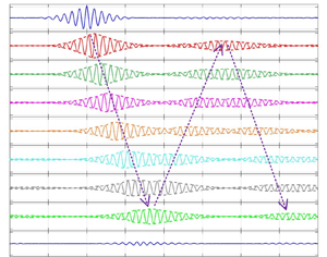
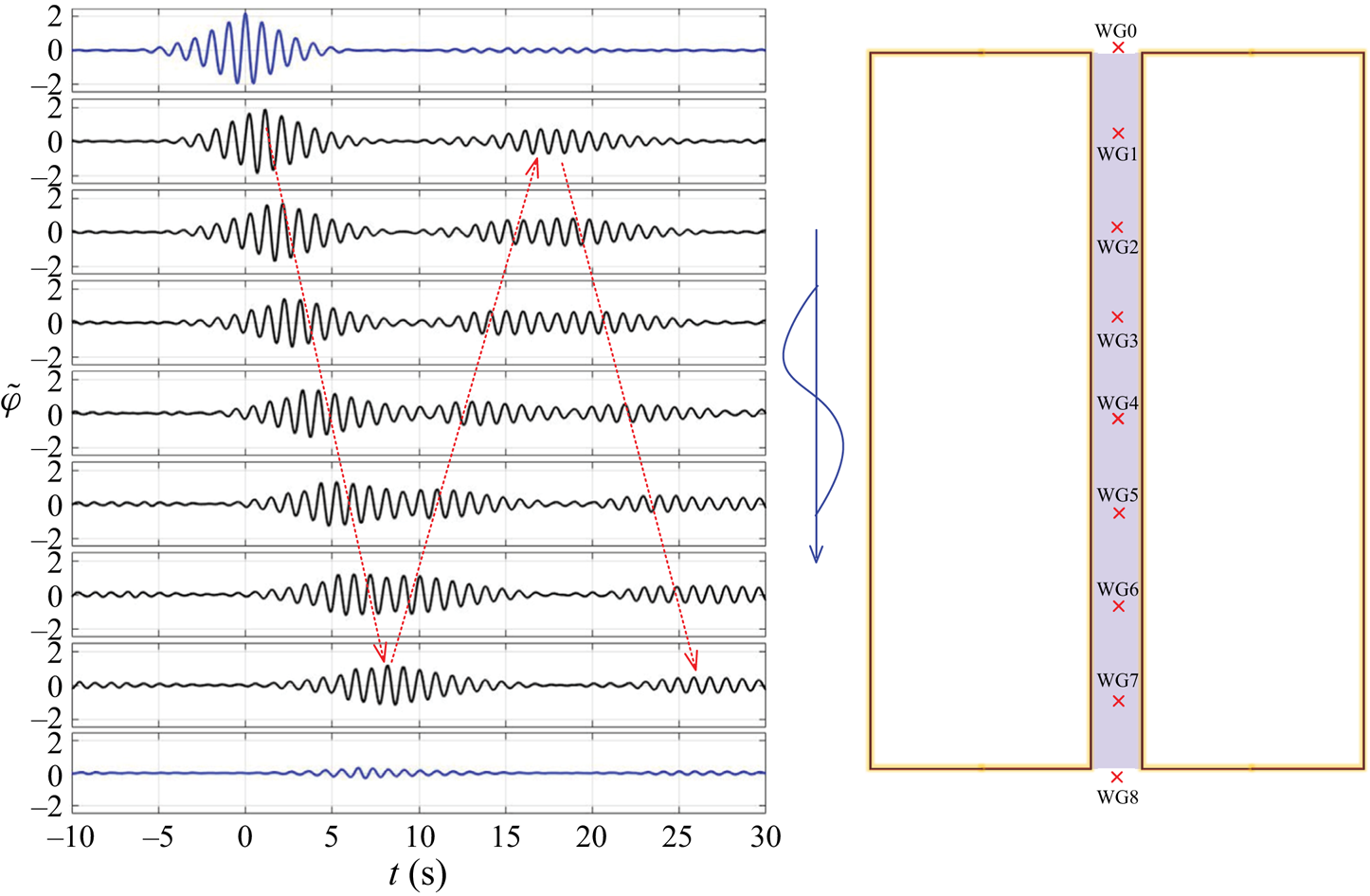
 $\sim$17 s) is associated with a maximum group propagating along the entire length of the gap and being reflected from the far end and returning to the upwave end. To demonstrate this process, figure 10 shows the NewResponse at WG0 propagating along the gap. The long time scale is associated with the new observation that the group velocity of the gap modes is much slower than that for free waves, as demonstrated in Reference Zhao, Taylor, Wolgamot, Molin and Eatock TaylorZhao et al. (Reference Zhao, Taylor, Wolgamot, Molin and Eatock Taylor2020).
NewResponse at WG0 (same as in figure 9) propagating along the gap in head sea excitation. The central red symbols refer to the location of the WG along the gap. The blue curves correspond to the WG at the ends of the gap, where they are nodes of the gap modes, and the black curves correspond to those inside the gap. As in figure 6, all the time histories have been normalised by the MPM of the incident wave.
The time histories in figures 6–9 have been again normalised by the MPM of the incident wave  $\alpha _{\eta }$, thus the peak of the NewResponse (blue dotted curve) actually indicates the amplification ( $=\alpha _{\varphi }/\alpha _{\eta }$) from the MPM in incident waves to that in the response. This information is important for engineering practice. For instance, one can estimate the MPM response immediately through this amplification ratio, once spectral information of the incident random wave field is given. One can see from the discussion in § 3 that the amplification ratio is derived from the linear transfer functions. The determination of the linear transfer functions does not depend on the shape of the incident wave spectrum, as long as this spectrum covers all the frequency components of interest.
5. Spatial variation of the response statistics along the gap
5.1. MPM along the gap
To investigate the statistics of the extreme resonances along the gap, we plot in figure 11 the amplification ratios ( $=\alpha _{\varphi }/\alpha _{\eta }$) at the seven WG inside the gap and the two gauges right at the ends. The amplification ratio is simply the magnitude of the peak 1 in $N$ gap response compared with the incident wave, both in the same random sea.
The (normalised) MPM of resonances along the gap under the excitation of the given sea state, (a) beam sea and (b) head sea. The red cross starlike symbols marked as ‘WG’ refer to the locations of the seven WG inside the gap and the remaining two installed 0.02 m beyond the gap ends. The length of the gap is represented as ‘L’, and ‘0’ in the horizontal axis represents the upwave end for head sea excitation. The shielded area refers to the outside of the gap. The hollow symbols represent responses allowing for laboratory-scale viscous damping as well as wave radiation, the solid symbols are for purely potential flow without viscous effects.
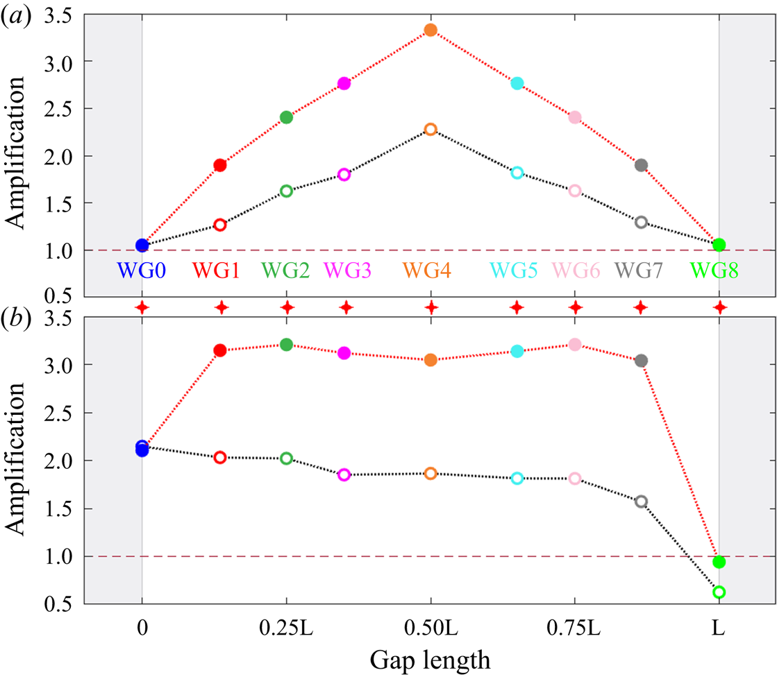
We stress that separate NewResponse calculations are done at every point in the gap and at the ends. For the beam sea excitation results shown in figure 11(a), the largest amplification occurs at the centre of the gap, reaching up to  $2.28 \times$ the MPM of the incident waves, and symmetrically decreases towards the ends of the gap where the ratio is around 1. The maximum gap elevation is consistently around $2\times \sim 2.3 \times$ the maximum incident waves, suggesting greenwater is unlikely to occur from the gap. However, this could induce significant motions on fenders, which are deployed in the gap to avoid collision between two side-by-side moored vessels.
It is worth noting that the amplifications are related to the choice of the spectral shape parameter  $\gamma$ and the peak frequency $f_p$ of the incident waves. It is interesting to see that the experimentally determined largest amplification determined in head sea excitation occurs at the upwave end of the gap, where it is close to a node for all the gap resonance modes. The large amplification at the upwave end is a result of a (end-shape dependent) local diffraction effect, where the surface elevations are locally controlled by diffraction around the ends of the boxes; the length of the gap and the gap modes locally do not matter.
Experimental (Reference Zhao, Wolgamot, Taylor and Eatock TaylorZhao et al., 2017) and numerical (Reference Wang, Wolgamot, Zhao, Draper, Taylor and ChengWang et al., 2019) studies have suggested that the viscous damping in the gap resonance problem is Stokes-type laminar boundary and has a linear form at the large model scale. The largest surface motions in the gap in our tests are  $\sim$5 cm at a frequency of $\sim$1.02 s $^{-1}$, giving a Reynolds number $R_{\delta }=u\sqrt {2/{(\omega {v})}}\approx 180$, so into the disturbed laminar regime discussed by Reference Blondeaux and VittoriBlondeaux and Vittori (Reference Blondeaux and Vittori2021). Using a Froude length scaling of 60, this would give a Reynolds number for the oscillatory boundary layers of $\sim$4000 for a 4 m gap in the field. This is well into the turbulent regime for a hydrodynamically smooth wall, but wall roughness would be present for vessels performing side-by-side transfers. The boundary layer behaviour is likely to be different at full scale in the field. It is hard to estimate how the effects of boundary layer damping will be changed until field measurements become available. However, it is expected that the viscous effects will be reduced, similar to the case of the circular cylinder in oscillatory flow (Reference SarpkayaSarpkaya, 1986), as Reynolds number increases. Therefore, the linear potential flow calculations (using the Oxford DIFFRACT code) provide an upper bound on the gap responses. These upper bounds account for the radiation damping of the gap modes but exclude viscous damping. We expect the field results may lie between those from the basin tests and the inviscid estimates, assuming the vessel sides can be treated as hydrodynamically smooth.
Similar to what has been done with the experimental data, we calculated the MPM responses along the gap using the linear transfer functions obtained from potential flow calculations. These numerical results (solid dots) are plotted on top of the experimental data, as shown in figure 11. It is seen that the numerical predictions in the beam sea condition are virtually a ‘stretched’ version of the experimental data, with data at the gap ends being fixed. This is not surprising, as the viscous damping plays a role at the resonances, where the gap ends are close to a node of each gap mode. In the head sea excitation, the numerical predictions are ‘stretched’ inside the gap and remain similar to the experimental data at the upwave end of the gap. However, it is interesting to note that the numerical prediction at the downwave end is slightly larger than that determined in the experiment. The response at the downwave end can be regarded as a combined contribution from the radiated wave from the gap and the scattered wave due to the two models as a whole. The latter contribution should be similar for the experiments and the simulations. For the former one, the waves inside the gap keep losing energy due to friction with the model hulls, when propagating from one end of the gap towards the other in the experiments. As an example, one can see this process (of losing energy) from figure 10. One would expect that the response at the downwave end should be even smaller for an equivalent ‘flat’ model – a gap ‘filled’ version of two side-by-side models. The amplification ratio is calculated to be 0.31 for an equivalent ‘flat’ model, smaller than that (0.63 as shown in figure 11) determined by experiments for two models with a gap.
We suggest that the reduced scale basin tests and the potential flow calculations provide lower and upper bounds on the gap responses at full scale.
5.2. Response structure given each MPM
In addition to the MPM responses at a specific location, it is also of practical interest to understand what the corresponding responses look like elsewhere. To simplify the demonstration, here we focus on the experimental data only. As shown in figure 12, the MPM responses are given by hollow circles, the maximum responses elsewhere along the gap under the same design wave are given by crosses in the same colour. It has been shown in § 4 that the MPM response at each different location is driven by a different design wave. Here, figure 12 shows that the maximum responses at a chosen point driven by design waves at points elsewhere on the structure is lower than that driven by the design wave for that specified point. Therefore, the hollow circles (MPM responses) – as in figure 11 – form an upper bounding envelope for all design waves – at the same return period.
Responses along the gap driven by design waves for each wave gauge location, (a) beam sea excitation and (b) head sea excitation. The cross starlike symbols marked as ‘WG’ refer to the locations of the WG. The hollow circle in each curve identifies the location of the wave gauge for which the design wave – exciting the responses along the gap – is given. The hollow circles, representing the MPM of the responses, are the same as in figure 11.

It is interesting to see that in the head sea excitation, the MPM response at a specified location is the maximum response along the gap under the same sea state. In contrast, the maximum response always occurs at the centre of the gap in the beam sea excitation, no matter where the MPM response (or design wave) is chosen. This may suggest the important role of the first gap mode in producing the MPM responses along the gap, in beam sea excitations.
6. Conclusions
Focusing on the statistics of gap resonances driven by linear wave excitation, analysis is performed on the extreme surface elevation motions within the gap. Two identical vessel models forming a narrow gap are fixed in the wave basin during the tests. In contrast to our previous studies (Reference Zhao, Taylor, Wolgamot, Molin and Eatock TaylorZhao et al., 2020, Reference Zhao, Wolgamot, Taylor and Eatock Taylor2017) which unravelled new physics, this study investigated the statistics of gap resonances and their spatial variation along the gap. The method is very time efficient, showing strong benefits to applications.
Transient wave groups are used to drive the gap resonant responses. The wave surface elevations are measured both inside the gap and at the ends, allowing for the investigation of the response statistics along the gap. Data recording was stopped just before the arrival of any waves reflected by the walls of the wave basin, therefore providing clean signals. The linear transfer functions of the water surface resonance along the narrow gap are obtained based on the experimental data. Only the odd gap modes are excited at the gap centre as a result of the symmetrical set-up in beam sea tests, while both odd and even gap modes are driven in the head sea condition as the symmetry is broken.
Based on the experimentally determined linear transfer functions, we identify a set of design waves that produce the complete time history of the MPM local response in a random sea. This shape is simply the autocorrelation function for response in the random wave field. The amplitude is set by the properties of the extremes of a narrow banded Gaussian variable, hence is Rayleigh distributed. This shows a slow build-up with a strong beating pattern in time followed by a rapid decay to zero. This is a reflection of the different gap resonance modes being excited during the build-up of the extreme response.
The statistics of the gap resonance extremes are sensitive to the headings: the MPM of gap resonance occurs at the centre of the gap for beam sea excitation, while for head sea excitation it is at the upwave end of the gap. The largest response at the upwave end is not influenced by the gap resonance, but is just a result of local diffraction by the ends of the boxes.
The application of this approach to problems of gap resonance at field scale is dependent on the modal damping. At wave basin scale, this is in the regime described as ‘disturbed laminar’ by Reference Blondeaux and VittoriBlondeaux and Vittori (Reference Blondeaux and Vittori2021) for Stokes oscillatory boundary layers on smooth walls, but at field scale these boundary layers will be turbulent, again for smooth walls. Although the actual damping at field scale remains unknown, we have presented upper bounds on the gap motions based on linear potential flow, so only with wave radiation damping included. This upper bound may be useful for decision making for offshore operations. This study has focused on linear excitation; however, it is possible to extend this time-efficient model to nonlinear excitation, e.g. second-order responses which will be tackled in a separate study.
It should be noted that the two vessel models are fixed during the model tests, and hence we have tackled a pure diffraction problem. In the case of floating vessels, the vessel motions will couple with the gap resonant responses, either enhancing or cancelling the vertical free-surface motion in the gap. Therefore, the pure diffraction problem is not necessarily the worst scenario. However, the tests with the fixed model facilitate the understanding of the statistics of gap resonances and the observations drawn from the experiments are insightful. As long the linear transfer functions for an offshore system are obtained, one can apply this approach to the problem of gap resonance between two moored floating bodies.
Acknowedgements
We gratefully acknowledge the comments from reviewers.
Funding Statement
This work was undertaken as part of the DECRA fellowship (grant no. DE190101296) awarded by the Australian Research Council. It was also supported by the Industrial Transformation Research Hub for Offshore Floating Facilities which is funded by the Australian Research Council, Woodside Energy, Shell, Bureau Veritas and Lloyd's Register (grant no. IH140100012).
Declaration of Interests
The authors report no conflict of interest.
Author Contributions
W.Z. and P.H.T. created the research plan and analysis methodology. H.A.W. calculated the numerical linear transfer functions, W.Z. wrote the manuscript and all the coauthors reviewed it.
Data Availability Statement
The data that support the findings of this study are available from the corresponding author (W.Z.).
Ethical Standards
The research meets all ethical guidelines, including adherence to the legal requirements of the study country.


 Open access