


1 Decision making in terms of utility maximization and the main message of the paper
The core idea of decision theory based on utility maximization is that an Agent models the world in terms of probability measure spaces and actions are identified with utility functions represented by random variables. A decision making Agent prefers the action that has the maximal expected utility with respect to the probability measure.
To be more explicit, let $(X,{\cal S},p)$
be a probability measure space, with X a set,
$(X,{\cal S},p)$
be a probability measure space, with X a set, ${\cal S}$
a
${\cal S}$
a $\sigma $
-field of some subsets of X and p a probability measure on
$\sigma $
-field of some subsets of X and p a probability measure on ${\cal S}$
. Real valued (
${\cal S}$
. Real valued ( ${\cal S}$
-measurable) random variables
${\cal S}$
-measurable) random variables $f_i\colon X\to \mathrm {I\!R}$
(
$f_i\colon X\to \mathrm {I\!R}$
( $i\in I$
) represent possible actions by an Agent, and the prescription of utility theory is: The Agent should choose action
$i\in I$
) represent possible actions by an Agent, and the prescription of utility theory is: The Agent should choose action $f_j$
for which
$f_j$
for which
 $$ \begin{align} \langle f_j\rangle_{p}> \langle f_i\rangle_{p}\quad \text{for all} i\not =j, \end{align} $$
where $\langle f\rangle _{p}\doteq \int f dp$
is the expectation value of f with respect to p (see the monographs [Reference Bradley3, Reference Fishburn10, Reference Gilboa11, Reference Kreps16] for the details and [Reference Briggs, Zalta and Nodelman4, Reference Buchak and Zalta6, Reference Chakrabarty and Kanaujiya7] for compact reviews of the main ideas and of some history of utility theory).
$\langle f\rangle _{p}\doteq \int f dp$
is the expectation value of f with respect to p (see the monographs [Reference Bradley3, Reference Fishburn10, Reference Gilboa11, Reference Kreps16] for the details and [Reference Briggs, Zalta and Nodelman4, Reference Buchak and Zalta6, Reference Chakrabarty and Kanaujiya7] for compact reviews of the main ideas and of some history of utility theory).
In the decision theoretic context elements in ${\cal S}$
are interpreted as states/properties of the world (equivalently: as propositions stating some properties of the world). The value
${\cal S}$
are interpreted as states/properties of the world (equivalently: as propositions stating some properties of the world). The value $f_j(x)$
is the utility (degree of preference) of the action
$f_j(x)$
is the utility (degree of preference) of the action $f_j$
from the Agent’s perspective if the state of the world is x (the larger
$f_j$
from the Agent’s perspective if the state of the world is x (the larger $f_j(x)$
the more the Agent prefers action
$f_j(x)$
the more the Agent prefers action $f_j$
if x obtains). The probability measure p can be viewed either as:
$f_j$
if x obtains). The probability measure p can be viewed either as:
-
(i) representing subjective degrees of belief of the Agent in the truth of the propositions in ${\cal S}$
; or as
${\cal S}$
; or as -
(ii) expressing objective features of the world (e.g., as frequencies with which the features of the world obtain).

If p is viewed subjectively, the expectation value $\langle f_j\rangle _{p}$
expresses the Agent’s subjective degree of expectation of the value of the action
$\langle f_j\rangle _{p}$
expresses the Agent’s subjective degree of expectation of the value of the action $f_j$
, and the Agent makes a rational decision if prefers
$f_j$
, and the Agent makes a rational decision if prefers $f_j$
because this choice is in harmony with his subjective expectation. If p is an objective probability (which we indicate below by using the notation
$f_j$
because this choice is in harmony with his subjective expectation. If p is an objective probability (which we indicate below by using the notation $p^*$
), say as relative frequency, then the Agent’s decision to prefer action
$p^*$
), say as relative frequency, then the Agent’s decision to prefer action $f_j$
is objectively good because (on average) the value of
$f_j$
is objectively good because (on average) the value of $f_j$
is objectively higher than the average value of
$f_j$
is objectively higher than the average value of $f_i$
, and
$f_i$
, and $\langle f_j\rangle _{p^*}> \langle f_i\rangle _{p^*}$
is an expression of this.
$\langle f_j\rangle _{p^*}> \langle f_i\rangle _{p^*}$
is an expression of this.
If in a decision situation there is both an objective probability $p^*$
that determines an objectively good decision and the Agent also has subjective degrees of belief p, then one would like a rational decision based on p to be also objectively good. But one cannot expect this to be the case in general because the Agent’s subjective probability p might differ from the objective probability
$p^*$
that determines an objectively good decision and the Agent also has subjective degrees of belief p, then one would like a rational decision based on p to be also objectively good. But one cannot expect this to be the case in general because the Agent’s subjective probability p might differ from the objective probability $p^*$
; hence the expectation values of the utility functions determined by
$p^*$
; hence the expectation values of the utility functions determined by $p^*$
might differ from the expectation values of the utility functions calculated by p. Being aware of this, the Agent can try to make an objectively good decision by adhering to the following 4-step strategy, to which we will refer as “conditioning strategy”:
$p^*$
might differ from the expectation values of the utility functions calculated by p. Being aware of this, the Agent can try to make an objectively good decision by adhering to the following 4-step strategy, to which we will refer as “conditioning strategy”:
-
(i) Get information about the values of the objective probability
$p^*$
on some elements in
${\cal S}$
. -
(ii) Update the subjective probability p by conditionalizing p on the acquired information about the objective probability
$p^*$
. -
(iii) Calculate the expectation values of the utility functions using the obtained conditional probability.
-
(iv) Make decision on the basis of the order of the expectation values of the utility functions calculated using the obtained conditional probability.


The problem we investigate in this paper is to what extent this conditional strategy succeeds in ensuring that a rational decision is objectively good indeed.
The main message of this paper is that this conditioning strategy is not reliable in the case of finite probability spaces. We will show that there exist decision situations represented by probability spaces having three and four elementary events with objective probabilities $p^*$
and subjective priors p such that no matter what evidence the Agent has about
$p^*$
and subjective priors p such that no matter what evidence the Agent has about $p^*$
, as long as the evidence is not the complete knowledge of
$p^*$
, as long as the evidence is not the complete knowledge of $p^*$
, the objectively good decision determined by
$p^*$
, the objectively good decision determined by $p^*$
cannot be obtained by calculating the expectation values of the utility functions using the updated version of the prior p, where the updating is Jeffrey conditionalizing on partial evidence about
$p^*$
cannot be obtained by calculating the expectation values of the utility functions using the updated version of the prior p, where the updating is Jeffrey conditionalizing on partial evidence about $p^*$
. We call such an objectively good decision conditionally p-inaccessible (Definition 3.2).
$p^*$
. We call such an objectively good decision conditionally p-inaccessible (Definition 3.2).
We also show that if a conditionally p-inaccessible decision exists in a finite probability space, then there exist uncountably many (namely, a continuum number of) conditionally p-inaccessible decisions in that probability space (Proposition 6.1). We conjecture that this situation is generic in the sense that conditionally inaccessible decisions exist in some probability spaces with arbitrary large finite number of elementary events (Conjecture 7.3); (dis)proving this conjecture remains an open problem however. Some further open problems about conditional p-inaccessibility are formulated in §7 (see Conjecture 7.2). §3 gives the technically explicit definition of conditional p-inaccessibility, §4 relates conditional p-inaccessibility to the presence of Bayes Blind Spots [Reference Rédei and Gyenis18, Reference Shattuck and Wagner22]. §5 contains several examples of conditionally inaccessible decisions. The closing section interprets the phenomenon of conditionally inaccessible decisions from the perspective of how a utility maximizing decision maker should handle the uncertainties expressed by a lack of complete knowledge of probabilities that determine objectively good decisions.
2 A potential difficulty for decision making based on utility maximization using probabilities inferred via conditioning
As indicated in the previous section, a difficulty of decision making based on utility maximization is that a rational decision by an Agent based on his degree of belief p might not be objectively good—if there is an objective probability $p^*$
that determines a good decision in the sense of utility maximization. This can happen if p differs from
$p^*$
that determines a good decision in the sense of utility maximization. This can happen if p differs from $p^*$
. If, in view of this difficulty, the Agent follows the conditioning strategy described in the previous section, the first step is to get some information about
$p^*$
. If, in view of this difficulty, the Agent follows the conditioning strategy described in the previous section, the first step is to get some information about $p^*$
. If the Agent finds out the value
$p^*$
. If the Agent finds out the value $p^*(A)$
on some element A in
$p^*(A)$
on some element A in ${\cal S}$
, then the Agent also knows the value of
${\cal S}$
, then the Agent also knows the value of $p^*$
on the Boolean subalgebra
$p^*$
on the Boolean subalgebra $(\emptyset ,A,A^{\perp }, X)$
of
$(\emptyset ,A,A^{\perp }, X)$
of ${\cal S}$
generated by A. More generally, in order to be able to follow the conditioning strategy, the Agent needs to know the values
${\cal S}$
generated by A. More generally, in order to be able to follow the conditioning strategy, the Agent needs to know the values $p^*(A)$
for elements A in some sub-
$p^*(A)$
for elements A in some sub- $\sigma $
-field
$\sigma $
-field ${\cal A}$
of
${\cal A}$
of ${\cal S}$
. In the second step the Agent infers the values of
${\cal S}$
. In the second step the Agent infers the values of $p^*$
for elements that are in
$p^*$
for elements that are in ${\cal S}$
but not in
${\cal S}$
but not in ${\cal A}$
from values
${\cal A}$
from values $p^*(A)$
(
$p^*(A)$
( $A\in {\cal A}$
) via the usual procedure of conditioning. In some more detail, this inference procedure is the following (see, e.g., Chapter 6 in [Reference Billingsley2], or any of [Reference Ash and Doleans-Dade1, Reference Rosenthal21, Reference Williams23] for the mathematical theory of conditioning with respect to
$A\in {\cal A}$
) via the usual procedure of conditioning. In some more detail, this inference procedure is the following (see, e.g., Chapter 6 in [Reference Billingsley2], or any of [Reference Ash and Doleans-Dade1, Reference Rosenthal21, Reference Williams23] for the mathematical theory of conditioning with respect to $\sigma $
-fields, and [Reference Nielsen17, Reference Rescorla19, Reference Rescorla20] for some philosophical analysis of conditioning with respect to
$\sigma $
-fields, and [Reference Nielsen17, Reference Rescorla19, Reference Rescorla20] for some philosophical analysis of conditioning with respect to $\sigma $
-fields).
$\sigma $
-fields).
Assume that the Agent’s prior degree of belief p on ${\cal S}$
is such that the restriction
${\cal S}$
is such that the restriction $p^{*}_{{\cal A}}$
of
$p^{*}_{{\cal A}}$
of $p^*$
to
$p^*$
to ${\cal A}$
is absolutely continuous with respect to the restriction
${\cal A}$
is absolutely continuous with respect to the restriction $p_{{\cal A}}$
of p to
$p_{{\cal A}}$
of p to ${\cal A}$
. Then by the Radon–Nikodym theorem there exists the Radon–Nikodym derivative
${\cal A}$
. Then by the Radon–Nikodym theorem there exists the Radon–Nikodym derivative $\frac {d p^{*}_{{\cal A}}}{d p_{{\cal A}}}$
of
$\frac {d p^{*}_{{\cal A}}}{d p_{{\cal A}}}$
of $p^{*}_{{\cal A}}$
with respect to
$p^{*}_{{\cal A}}$
with respect to $p_{{\cal A}}$
: the (
$p_{{\cal A}}$
: the ( ${\cal A}$
-measurable) function
${\cal A}$
-measurable) function $\frac {d p^{*}_{{\cal A}}}{d p_{{\cal A}}}$
is the density function of
$\frac {d p^{*}_{{\cal A}}}{d p_{{\cal A}}}$
is the density function of $p^{*}_{{\cal A}}$
with respect to
$p^{*}_{{\cal A}}$
with respect to $p_{{\cal A}}$
, which gives
$p_{{\cal A}}$
, which gives $p^{*}_{{\cal A}}$
on
$p^{*}_{{\cal A}}$
on ${\cal A}$
as
${\cal A}$
as
 $$ \begin{align} p^{*}_{{\cal A}}(A)=\int \chi_A \frac{d p^{*}_{{\cal A}}}{d p_{{\cal A}}} d p_{{\cal A}} \qquad A\in{\cal A} \end{align} $$
( $\chi _A$
above denotes the characteristic (indicator) function of the set A; more generally below we will use
$\chi _A$
above denotes the characteristic (indicator) function of the set A; more generally below we will use $\chi _Z$
to denote the characteristic function of a set Z in
$\chi _Z$
to denote the characteristic function of a set Z in ${\cal S}$
). The formula (2) allows one to extend
${\cal S}$
). The formula (2) allows one to extend $p^{*}_{{\cal A}}$
from
$p^{*}_{{\cal A}}$
from ${\cal A}$
to a probability measure
${\cal A}$
to a probability measure $p^{*}_{p,{\cal A}}$
on
$p^{*}_{p,{\cal A}}$
on ${\cal S}$
by defining
${\cal S}$
by defining
 $$ \begin{align} p^{*}_{p,{\cal A}}(B)\doteq \int \chi_B \frac{d p^{*}_{{\cal A}}}{d p_{{\cal A}}} d p \qquad B\in{\cal S.} \end{align} $$
Remark 2.1. If the subalgebra ${\cal A}$
is generated by a countable partition
${\cal A}$
is generated by a countable partition $\{A_i\}_{i\in \mathrm {I\!N}}$
and
$\{A_i\}_{i\in \mathrm {I\!N}}$
and $p_{{\cal A}}(A_i)=p(A_i)\not =0$
for all
$p_{{\cal A}}(A_i)=p(A_i)\not =0$
for all $i\in \mathrm {I\!N}$
, then
$i\in \mathrm {I\!N}$
, then $\frac {d p^{*}_{{\cal A}}}{d p_{{\cal A}}}$
isFootnote
1
$\frac {d p^{*}_{{\cal A}}}{d p_{{\cal A}}}$
isFootnote
1
 $$ \begin{align} \frac{d p^{*}_{{\cal A}}}{d p_{{\cal A}}}(x)=\sum_{i\in\mathrm{I\!N}} \frac{p^{*}_{{\cal A}}(A_i)}{p_{{\cal A}}(A_i)} \chi_{A_i}(x) \qquad x\in X. \end{align} $$
The probability $p^{*}_{p,{\cal A}}(B)$
defined by (3) with the density function
$p^{*}_{p,{\cal A}}(B)$
defined by (3) with the density function $\frac {d p^{*}_{{\cal A}}}{d p_{{\cal A}}}$
in (4) has the form:
$\frac {d p^{*}_{{\cal A}}}{d p_{{\cal A}}}$
in (4) has the form:
 $$ \begin{align} p^{*}_{p,{\cal A}}(B)&\doteq \int \lbrack\chi_B \sum_{i\in\mathrm{I\!N}} \frac{p^{*}_{{\cal A}}(A_i)}{p_{{\cal A}}(A_i)} \chi_{A_i}\rbrack d p\nonumber\\
&= \sum_{i\in\mathrm{I\!N}} \frac{p^{*}_{{\cal A}}(A_i)}{p_{{\cal A}}(A_i)} \int\chi_B\chi_{A_i} d p \nonumber\\
&= \sum_{i\in\mathrm{I\!N}} \frac{p^{*}_{{\cal A}}(A_i)}{p_{{\cal A}}(A_i)} p(B\cap A_i)\nonumber\\
&=\sum_{i\in\mathrm{I\!N}} \frac{p(B\cap A_i)}{p(A_i)} p^{*}_{{\cal A}}(A_i)\nonumber\\
&= \sum_{i\in\mathrm{I\!N}} p(B|A_i) p^{*}_{{\cal A}}(A_i). \end{align} $$
$$ \begin{align} p^{*}_{p,{\cal A}}(B)&\doteq \int \lbrack\chi_B \sum_{i\in\mathrm{I\!N}} \frac{p^{*}_{{\cal A}}(A_i)}{p_{{\cal A}}(A_i)} \chi_{A_i}\rbrack d p\nonumber\\
&= \sum_{i\in\mathrm{I\!N}} \frac{p^{*}_{{\cal A}}(A_i)}{p_{{\cal A}}(A_i)} \int\chi_B\chi_{A_i} d p \nonumber\\
&= \sum_{i\in\mathrm{I\!N}} \frac{p^{*}_{{\cal A}}(A_i)}{p_{{\cal A}}(A_i)} p(B\cap A_i)\nonumber\\
&=\sum_{i\in\mathrm{I\!N}} \frac{p(B\cap A_i)}{p(A_i)} p^{*}_{{\cal A}}(A_i)\nonumber\\
&= \sum_{i\in\mathrm{I\!N}} p(B|A_i) p^{*}_{{\cal A}}(A_i). \end{align} $$
The formula (5) is known in the philosophical literature as “Jeffrey conditioning” [Reference Jeffrey14, Reference Jeffrey15] (the terminology “probability kinematics” is also used to refer to Jeffrey conditioning, see [Reference Diaconis and Zabell9]). If X in the probability space $(X,{\cal S},p^{*})$
has a finite number of elements, then
$(X,{\cal S},p^{*})$
has a finite number of elements, then $p^{*}_{p,{\cal A}}(B)$
is always of the form (5) (with a finite summation). For a compact summary of the basic features of Jeffrey conditioning see [Reference Shattuck and Wagner22]. From now on we assume that the set of elementary events is finite, having n elements:
$p^{*}_{p,{\cal A}}(B)$
is always of the form (5) (with a finite summation). For a compact summary of the basic features of Jeffrey conditioning see [Reference Shattuck and Wagner22]. From now on we assume that the set of elementary events is finite, having n elements: $X_n$
. See Remark 7.4 on the case of infinite probability spaces. In case of finite probability spaces we also assume that
$X_n$
. See Remark 7.4 on the case of infinite probability spaces. In case of finite probability spaces we also assume that ${\cal S}$
is the full power set of
${\cal S}$
is the full power set of $X_n$
and we refer to
$X_n$
and we refer to ${\cal S}$
and
${\cal S}$
and ${\cal A}$
as Boolean algebras rather than
${\cal A}$
as Boolean algebras rather than $\sigma $
-fields.
$\sigma $
-fields.
Having inferred $p^{*}_{p,{\cal A}}$
from the values of
$p^{*}_{p,{\cal A}}$
from the values of $p^{*}$
on the elements of
$p^{*}$
on the elements of ${\cal A}$
as evidence, the Agent can use
${\cal A}$
as evidence, the Agent can use $p^{*}_{p,{\cal A}}$
to calculate the expectation values
$p^{*}_{p,{\cal A}}$
to calculate the expectation values $\langle f_{i} \rangle _{p^{*}_{p,{\cal A}}}$
of the utility functions
$\langle f_{i} \rangle _{p^{*}_{p,{\cal A}}}$
of the utility functions $f_i$
and can base the decision on the relation of the expectation values
$f_i$
and can base the decision on the relation of the expectation values $\langle f_{i} \rangle _{p^{*}_{p,{\cal A}}}$
. One potential difficulty such decision making has to face is that, although the inferred (conditional) probability measure
$\langle f_{i} \rangle _{p^{*}_{p,{\cal A}}}$
. One potential difficulty such decision making has to face is that, although the inferred (conditional) probability measure $p^{*}_{p,{\cal A}}$
coincides with the objective probability
$p^{*}_{p,{\cal A}}$
coincides with the objective probability $p^{*}$
on all elements in
$p^{*}$
on all elements in ${\cal A}$
, the inferred probability
${\cal A}$
, the inferred probability $p^{*}_{p,{\cal A}}$
might not be equal to the objective probability on all other elements in
$p^{*}_{p,{\cal A}}$
might not be equal to the objective probability on all other elements in ${\cal S}$
; so, in general, one can have
${\cal S}$
; so, in general, one can have $p^{*}\not = p^{*}_{p,{\cal A}}$
. Thus it might happen that
$p^{*}\not = p^{*}_{p,{\cal A}}$
. Thus it might happen that $\langle f_i \rangle _{p^{*}_{p,{\cal A}}}\not = \langle f_i \rangle _{p^{*}}$
. Consequently, it is not obvious that the rational decision between
$\langle f_i \rangle _{p^{*}_{p,{\cal A}}}\not = \langle f_i \rangle _{p^{*}}$
. Consequently, it is not obvious that the rational decision between $f_i$
and
$f_i$
and $f_j$
based on considering the expectation values of
$f_j$
based on considering the expectation values of $f_i$
and
$f_i$
and $f_j$
calculated using the inferred probability
$f_j$
calculated using the inferred probability $p^{*}_{p,{\cal A}}$
is objectively good in the sense that it coincides with the decision based on considering the expectation values of
$p^{*}_{p,{\cal A}}$
is objectively good in the sense that it coincides with the decision based on considering the expectation values of $f_i$
and
$f_i$
and $f_j$
calculated using the objective probability
$f_j$
calculated using the objective probability $p^{*}$
. That is to say, it is not obvious that
$p^{*}$
. That is to say, it is not obvious that
 $$ \begin{align} \langle f_i \rangle_{p^{*}}> \langle f_j \rangle_{p^{*}} \quad \text{entails} \quad \langle f_i \rangle_{p^{*}_{p,{\cal A}}}> \langle f_j \rangle_{p^{*}_{p,{\cal A}}}. \end{align} $$
The next section formulates the possibility of violation of the entailment in (6) in terms of two definitions, restricted to the case of two utility functions.
3 Conditionally inaccessible decisions—definition
Given a probability space $(X_n,{\cal S},p^{*})$
and two random variables
$(X_n,{\cal S},p^{*})$
and two random variables $f_1,f_2\colon X_n\to \mathrm {I\!R}$
, we call
$f_1,f_2\colon X_n\to \mathrm {I\!R}$
, we call
 $$ \begin{align} \big\langle(X_n,{\cal S},p^{*}),f_1,f_2\big\rangle \end{align} $$
a decision context and the inequality $\langle f_1 \rangle _{p^{*}}> \langle f_2 \rangle _{p^{*}}$
a decision. We call the decision context trivial if
$\langle f_1 \rangle _{p^{*}}> \langle f_2 \rangle _{p^{*}}$
a decision. We call the decision context trivial if $f_1(x)>f_2(x)$
for all x in
$f_1(x)>f_2(x)$
for all x in $X_n$
. In a trivial decision context it is obvious that
$X_n$
. In a trivial decision context it is obvious that $\langle f_1 \rangle _{q}> \langle f_2 \rangle _{q}$
for every probability measure q on
$\langle f_1 \rangle _{q}> \langle f_2 \rangle _{q}$
for every probability measure q on ${\cal S}$
; hence in such situations it is obvious that
${\cal S}$
; hence in such situations it is obvious that $f_1$
is preferred to
$f_1$
is preferred to $f_2$
no matter what the objective and subjective probabilities are. To avoid such trivial decision situations, in what follows we assume that all decision contexts are non-trivial.
$f_2$
no matter what the objective and subjective probabilities are. To avoid such trivial decision situations, in what follows we assume that all decision contexts are non-trivial.
A Boolean subalgebra ${\cal A}$
of
${\cal A}$
of ${\cal S}$
is called proper and non-trivial if
${\cal S}$
is called proper and non-trivial if ${\cal A}\subset {\cal S}$
and
${\cal A}\subset {\cal S}$
and ${\cal A}\not =\{\emptyset ,X_n\}$
(note that
${\cal A}\not =\{\emptyset ,X_n\}$
(note that $\subset $
designates the proper subset relation).
$\subset $
designates the proper subset relation).
Definition 3.1. Given a decision context $\big \langle (X_n,{\cal S},p^{*}),f_1,f_2\big \rangle $
, we say that the decision
$\big \langle (X_n,{\cal S},p^{*}),f_1,f_2\big \rangle $
, we say that the decision
 $$ \begin{align} \langle f_1 \rangle_{p^{*}}> \langle f_2 \rangle_{p^{*}} \end{align} $$
is conditionally $(p,{\cal A})$
-inaccessible if
$(p,{\cal A})$
-inaccessible if
-
•
${\cal A}$
is a proper, non-trivial Boolean subalgebra of
${\cal S}$
; -
•
$p$
is a probability measure on
${\cal S}$
(prior) such that the restriction
$p^{*}_{{\cal A}}$
of
$p^{*}$
to
${\cal A}$
is absolutely continuous with respect to the restriction
$p_{{\cal A}}$
of
$p$
to
${\cal A}$
; -
• and we have:
(9)where
$$ \begin{align} \langle f_1 \rangle_{p^{*}_{p,{\cal A}}} \leq \langle f_2 \rangle_{p^{*}_{p,{\cal A}}}, \end{align} $$
$p^{*}_{p,{\cal A}}$
is the conditional probability measure defined by (3).


We call the decision conditionally $(p,{\cal A})$
-accessible if it is not conditionally
$(p,{\cal A})$
-accessible if it is not conditionally $(p,{\cal A})$
-inaccessible.
$(p,{\cal A})$
-inaccessible.
The content of conditional $(p,{\cal A})$
-inaccessibility is that the Agent cannot reach the right decision determined by the objective probability if the information available for the Agent are the values of the objective probability on the subalgebra
$(p,{\cal A})$
-inaccessibility is that the Agent cannot reach the right decision determined by the objective probability if the information available for the Agent are the values of the objective probability on the subalgebra ${\cal A}$
, and the Agent calculates the expectation values of utility functions using conditional probabilities obtained from the partial information available and using prior p: either the Agent cannot make a decision between
${\cal A}$
, and the Agent calculates the expectation values of utility functions using conditional probabilities obtained from the partial information available and using prior p: either the Agent cannot make a decision between $f_1$
and
$f_1$
and $f_2$
because the Agent is indifferent between actions
$f_2$
because the Agent is indifferent between actions $f_1$
and
$f_1$
and $f_2$
(if there is equality in (9)), or the decision made this way by the Agent is objectively wrong (when there is strict inequality in (9)).
$f_2$
(if there is equality in (9)), or the decision made this way by the Agent is objectively wrong (when there is strict inequality in (9)).
A natural strengthening of Definition 3.1 is as follows.
Definition 3.2. Given a decision context $\big \langle (X_n,{\cal S},p^{*}),f_1,f_2\big \rangle $
, we say that the decision
$\big \langle (X_n,{\cal S},p^{*}),f_1,f_2\big \rangle $
, we say that the decision $\langle f_1 \rangle _{p^{*}}> \langle f_2 \rangle _{p^{*}}$
is conditionally
$\langle f_1 \rangle _{p^{*}}> \langle f_2 \rangle _{p^{*}}$
is conditionally $p$
-inaccessible if it is conditionally
$p$
-inaccessible if it is conditionally $(p,{\cal A})$
-inaccessible (in the sense of Definition 3.1) for all (proper, non-trivial) subalgebras
$(p,{\cal A})$
-inaccessible (in the sense of Definition 3.1) for all (proper, non-trivial) subalgebras ${\cal A}$
of
${\cal A}$
of ${\cal S}$
.
${\cal S}$
.
The content of p-inaccessibility specified by Definition 3.2 is that the prior p of the Agent makes it impossible for the Agent to reach the objectively good decision if the Agent follows the conditioning strategy described earlier in §1: if the Agent calculates the expectation values of the utility functions using probabilities inferred via conditionalizing his prior p on partial information about the objective probability, then either the Agent cannot make a decision between $f_1$
and
$f_1$
and $f_2$
(because the Agent is indifferent between
$f_2$
(because the Agent is indifferent between $f_1$
and
$f_1$
and $f_2$
), or the decision the Agent makes will be objectively wrong—no matter what partial information the Agent has about the objective probability.
$f_2$
), or the decision the Agent makes will be objectively wrong—no matter what partial information the Agent has about the objective probability.
Given the definition of conditional p-inaccessibility of decisions, one is led to the following.
Problem 3.3. Under what conditions on the decision context $\big \langle (X_n,{\cal S},p^{*}),f_1,f_2\big \rangle $
, and for which
$\big \langle (X_n,{\cal S},p^{*}),f_1,f_2\big \rangle $
, and for which $p$
does it happen that the decision
$p$
does it happen that the decision $\langle f_1 \rangle _{p^{*}}> \langle f_2 \rangle _{p^{*}}$
is conditionally
$\langle f_1 \rangle _{p^{*}}> \langle f_2 \rangle _{p^{*}}$
is conditionally $p$
-inaccessible?
$p$
-inaccessible?
4 Conditionally inaccessible decisions and the Bayes Blind Spot
Clearly, conditional p-inaccessibility of the decision $\langle f_1 \rangle _{p^{*}}> \langle f_2 \rangle _{p^{*}}$
is a much stronger property than conditional
$\langle f_1 \rangle _{p^{*}}> \langle f_2 \rangle _{p^{*}}$
is a much stronger property than conditional $(p,{\cal A})$
-inaccessibility for some
$(p,{\cal A})$
-inaccessibility for some ${\cal A}$
, and conditional p-inaccessibility can only occur if
${\cal A}$
, and conditional p-inaccessibility can only occur if $p^{*}$
belongs to the set of probability measures on
$p^{*}$
belongs to the set of probability measures on ${\cal S}$
that form what is called the “Bayes Blind Spot” of p: The Bayes Blind Spot of p is the set of probability measures on
${\cal S}$
that form what is called the “Bayes Blind Spot” of p: The Bayes Blind Spot of p is the set of probability measures on ${\cal S}$
that are absolutely continuous with respect to p, yet they cannot be obtained as conditional probabilities from incomplete evidence using p as prior [Reference Gyenis and Rédei13, Reference Rédei and Gyenis18]. That is to say, probability measure
${\cal S}$
that are absolutely continuous with respect to p, yet they cannot be obtained as conditional probabilities from incomplete evidence using p as prior [Reference Gyenis and Rédei13, Reference Rédei and Gyenis18]. That is to say, probability measure $p^{*}$
is in the p-Bayes Blind Spot if it is absolutely continuous with respect to p but cannot be written in the form of (3) for any proper, non-trivial subalgebra
$p^{*}$
is in the p-Bayes Blind Spot if it is absolutely continuous with respect to p but cannot be written in the form of (3) for any proper, non-trivial subalgebra ${\cal A}$
.
${\cal A}$
.
It is known that the p-Bayes Blind Spot is not empty for a lot of p in typical probability spaces; in fact the p-Bayes Blind Spot is known to be a very large set for every p in all finite probability spaces: the Bayes Blind Spot
“ $\ldots $
has the same cardinality as the set of all probability measures (continuum); it has the same measure as the measure of the set of all probability measures (in the natural measure on the set of all probability measures); and is a ‘fat’ (second Baire category) set in topological sense in the set of all probability measures taken with its natural topology.” [Reference Rédei and Gyenis18, p. 3801].
$\ldots $
has the same cardinality as the set of all probability measures (continuum); it has the same measure as the measure of the set of all probability measures (in the natural measure on the set of all probability measures); and is a ‘fat’ (second Baire category) set in topological sense in the set of all probability measures taken with its natural topology.” [Reference Rédei and Gyenis18, p. 3801].
The p-Bayes Blind Spot is known to be large also in probability spaces where X is countably generated [Reference Shattuck and Wagner22].
Thus, a necessary condition for the existence of conditionally p-inaccessible decisions does hold in typical probability spaces. But this necessary condition is not sufficient: $p^{*}\not =p^{*}_{p,{\cal A}}$
does not entail that the decision
$p^{*}\not =p^{*}_{p,{\cal A}}$
does not entail that the decision $\langle f_1 \rangle _{p^{*}}> \langle f_2 \rangle _{p^{*}}$
is conditionally p-inaccessible. One can have a situation in which
$\langle f_1 \rangle _{p^{*}}> \langle f_2 \rangle _{p^{*}}$
is conditionally p-inaccessible. One can have a situation in which $p^{*}$
is in the p-Bayes Blind Spot but the decision is conditionally
$p^{*}$
is in the p-Bayes Blind Spot but the decision is conditionally $(p,{\cal A})$
-accessible for some
$(p,{\cal A})$
-accessible for some ${\cal A}$
and not conditionally
${\cal A}$
and not conditionally $(p,{\cal A}')$
-accessible for some other
$(p,{\cal A}')$
-accessible for some other ${\cal A}'\not ={\cal A}$
(see Remark 5.1). It can even happen that
${\cal A}'\not ={\cal A}$
(see Remark 5.1). It can even happen that $p^{*}$
is in the p-Bayes Blind Spot but the decision is conditionally
$p^{*}$
is in the p-Bayes Blind Spot but the decision is conditionally $(p,{\cal A})$
-accessible for all
$(p,{\cal A})$
-accessible for all ${\cal A}$
(see Example 5.4). That
${\cal A}$
(see Example 5.4). That $p^{*}$
lies in the p Bayes Blind Spot is not sufficient for conditional p-inaccessibility of a decision is not surprising because conditional p-inaccessibility depends sensitively not only on
$p^{*}$
lies in the p Bayes Blind Spot is not sufficient for conditional p-inaccessibility of a decision is not surprising because conditional p-inaccessibility depends sensitively not only on $p^{*}$
and on the prior p but also on the utility functions
$p^{*}$
and on the prior p but also on the utility functions $f_1, f_2$
. For this reason, finding a compact and useful general sufficient condition for conditional p- and
$f_1, f_2$
. For this reason, finding a compact and useful general sufficient condition for conditional p- and $(p,{\cal A})$
-inaccessibility seems a difficult problem. At any rate we are not able to give such a general sufficient condition.
$(p,{\cal A})$
-inaccessibility seems a difficult problem. At any rate we are not able to give such a general sufficient condition.
Given the lack of a general sufficient condition for conditional p- and $(p,{\cal A})$
-inaccessibility, it is not even obvious that decision contexts displaying conditional
$(p,{\cal A})$
-inaccessibility, it is not even obvious that decision contexts displaying conditional $(p,{\cal A})$
- (and especially) p-inaccessibility exist. In the next section we give examples of conditional
$(p,{\cal A})$
- (and especially) p-inaccessibility exist. In the next section we give examples of conditional $(p,{\cal A})$
- and p-accessibility in probability spaces having three and four elementary events. The examples involve elementary but tedious numerical calculations. To facilitate checking the correctness of those calculations, two short computer programs are available at https://doi.org/10.5281/zenodo.16789231. The first programme can be used to check the calculations in the probability spaces having three, and the second program in probability spaces having four elementary events. The programs can be run on online platforms such as https://sagecell.sagemath.org. We thank Z. Gyenis for providing the code for the computer programs.
$(p,{\cal A})$
- and p-accessibility in probability spaces having three and four elementary events. The examples involve elementary but tedious numerical calculations. To facilitate checking the correctness of those calculations, two short computer programs are available at https://doi.org/10.5281/zenodo.16789231. The first programme can be used to check the calculations in the probability spaces having three, and the second program in probability spaces having four elementary events. The programs can be run on online platforms such as https://sagecell.sagemath.org. We thank Z. Gyenis for providing the code for the computer programs.
5 Conditionally inaccessible decisions—examples in finite probability spaces
5.1 Example of a conditionally
$(p,{\cal A})$
-inaccessible decision in a probability space having three elementary events

Consider the decision context described by Table 1 (with $p^{*}$
as objective probability and p as prior probability).
$p^{*}$
as objective probability and p as prior probability). $(p,{\cal A})$
-inaccessibility,
$(p,{\cal A})$
-inaccessibility, $n=3$
$n=3$

Table 1 Long description
Column headers from left to right are X sub 3, x sub 1, x sub 2, x sub 3. The first row lists p star with values one all over eight, one all over four, and five all over eight. The second row lists f sub 1 with values negative two, negative two, and nine. The third row lists f sub 2 with values negative two, eight, and negative two. The fourth row lists italic p with values one all over twenty, nine all over ten, and one all over twenty. The table caption indicates p comma calligraphic A inaccessibility for n equals three.
Simple calculations show that the objectively good decision is
 $$ \begin{align} 4 \frac{7}{8}=\langle f_1 \rangle_{p^{*}}> \langle f_2 \rangle_{p^{*}}= \frac{1}{2}. \end{align} $$
In the case of a three-element set $X_3$
there are three non-trivial proper sub-Boolean algebras of the power set of
$X_3$
there are three non-trivial proper sub-Boolean algebras of the power set of $X_3$
, they are generated by three partitions:
$X_3$
, they are generated by three partitions:
 $$ \begin{align} &{\cal A}_1\quad \text{generated by}\quad \{\{x_1\},\{x_2,x_3\}\} \end{align} $$
 $$ \begin{align} &{\cal A}_2\quad \text{generated by}\quad \{\{x_2\},\{x_1,x_3\}\} \end{align} $$
 $$ \begin{align} &{\cal A}_3\quad \text{generated by}\quad \{\{x_3\},\{x_1,x_2\}\}. \end{align} $$
The Radon–Nikodym derivatives $\frac {dp^{*}_{{\cal A}_i}}{dp_{{\cal A}_i}}$
(
$\frac {dp^{*}_{{\cal A}_i}}{dp_{{\cal A}_i}}$
( $i=1,2,3$
) (see Remark 2.1, especially eq. (5)) are given in Table 2.
$i=1,2,3$
) (see Remark 2.1, especially eq. (5)) are given in Table 2.
Radon–Nikodym derivatives

Table 2 Long description
The header row lists four columns: X sub 3, x sub 1, x sub 2, and x sub 3. The first row shows the derivative d p star A sub 1 all over d p A sub 1, with values 2 and one half for x sub 1, thirty-five all over thirty-eight for x sub 2 and x sub 3. The second row presents d p star A sub 2 all over d p A sub 2, with values seven and one half for x sub 1, five all over eighteen for x sub 2, and seven and one half for x sub 3. The third row displays d p star A sub 3 all over d p A sub 3, with values fifteen all over thirty-eight for x sub 1 and x sub 2, and twelve and one half for x sub 3.
So one can calculate the expectation values of $f_1,f_2$
with respect to the inferred probabilities
$f_1,f_2$
with respect to the inferred probabilities $p^{*}_{p,{\cal A}_i}$
(
$p^{*}_{p,{\cal A}_i}$
( $i=1,2,3$
):
$i=1,2,3$
):
 $$ \begin{align} \langle f_1 \rangle_{p^{*}_{p,{\cal A}_i}}&=\sum_{j=1}^3 f_1(x_j)\frac{dp^{*}_{{\cal A}_i}}{dp_{{\cal A}_i}}(x_j)p(x_j)\quad i=1,2,3 \end{align} $$
 $$ \begin{align} \langle f_2 \rangle_{p^{*}_{p,{\cal A}_i}}&=\sum_{j=1}^3 f_2(x_j)\frac{dp^{*}_{{\cal A}_i}}{dp_{{\cal A}_i}}(x_j)p(x_j)\quad i=1,2,3. \end{align} $$
The results are given in Table 3.
Expectation values of utility functions

Table 3 Long description
The table has three rows, each corresponding to a utility function: A sub 1, A sub 2, and A sub 3. For A sub 1, the expectation value of f sub 1 is negative one and seventy-five over one hundred fifty-two, and for f sub 2 it is six and eleven over thirty-eight. For A sub 2, the expectation value of f sub 1 is two and one eighth, and for f sub 2 it is one half. For A sub 3, the expectation value of f sub 1 is four and seven eighths, and for f sub 2 it is one and twenty-one over thirty-eight. All values are listed under their respective columns for f sub 1 and f sub 2.
Thus we have the following ordering of the expected utilities calculated using the inferred probabilities:
 $$ \begin{align} \langle f_1 \rangle_{p^{*}_{p,{\cal A}_1}} &< \langle f_2 \rangle_{p^{*}_{p,{\cal A}_1}} \end{align} $$
 $$ \begin{align} \langle f_1 \rangle_{p^{*}_{p,{\cal A}_2}} &> \langle f_2 \rangle_{p^{*}_{p,{\cal A}_2}} \end{align} $$
 $$ \begin{align} \langle f_1 \rangle_{p^{*}_{p,{\cal A}_3}} &> \langle f_2 \rangle_{p^{*}_{p,{\cal A}_3.}} \end{align} $$
The inequality (16) means that the decision (10) is conditionally $(p,{\cal A}_1)$
-inaccessible; the inequality (17) means that the decision (10) is conditionally
$(p,{\cal A}_1)$
-inaccessible; the inequality (17) means that the decision (10) is conditionally $(p,{\cal A}_2)$
-accessible; and the inequality (18) means that the decision (10) is conditionally
$(p,{\cal A}_2)$
-accessible; and the inequality (18) means that the decision (10) is conditionally $(p,{\cal A}_3)$
-accessible.
$(p,{\cal A}_3)$
-accessible.
Remark 5.1. The decision (10) is not conditionally $p$
-inaccessible because the decision is not conditionally
$p$
-inaccessible because the decision is not conditionally $(p,{\cal A}_i)$
-inaccessible for
$(p,{\cal A}_i)$
-inaccessible for $i=2,3$
: the decision between
$i=2,3$
: the decision between $f_1$
and
$f_1$
and $f_2$
based on the relation of their expectation values expressed by the inequalities (17) and (18) is the same as the decision (10) based on
$f_2$
based on the relation of their expectation values expressed by the inequalities (17) and (18) is the same as the decision (10) based on $p^{*}$
. Yet, the objective probability
$p^{*}$
. Yet, the objective probability $p^{*}$
lies in the Bayes Blind Spot of
$p^{*}$
lies in the Bayes Blind Spot of $p$
: It is known (Proposition 3.1 in [Reference Rédei and Gyenis18]) that
$p$
: It is known (Proposition 3.1 in [Reference Rédei and Gyenis18]) that $p^{*}$
is in the
$p^{*}$
is in the $p$
-Bayes Blind Spot if and only if the Radon–Nikodym derivative
$p$
-Bayes Blind Spot if and only if the Radon–Nikodym derivative $\frac {dp^{*}}{dp}$
is an injective function. This holds for
$\frac {dp^{*}}{dp}$
is an injective function. This holds for $p^{*}$
and
$p^{*}$
and $p$
in this example:
$p$
in this example:
 $$ \begin{align} \frac{dp^{*}}{dp}(x_1)&=\frac{p^{*}(\{x_1\})}{p(\{x_1\})}=2 \frac{1}{2}\end{align} $$
 $$ \begin{align} \frac{dp^{*}}{dp}(x_2)&=\frac{p^{*}(\{x_2\})}{p(\{x_2\})}=\frac{5}{18}\end{align} $$
 $$ \begin{align} \frac{dp^{*}}{dp}(x_3)&=\frac{p^{*}(\{x_3\})}{p(\{x_3\})}=12 \frac{1}{2}. \end{align} $$
5.2 Example of a conditionally
$p$
-inaccessible decision with the uniform
$p$
in a probability space having three elementary events


Consider the decision context described in Table 4.
Conditionally p-inaccessible decision, $n=3$
, uniform prior
$n=3$
, uniform prior

Table 4 Long description
The table has four columns labeled from left to right as X sub 3, x sub 1, x sub 2, and x sub 3. The first row under X sub 3 is p-star, with values two all over ten for x sub 1, three all over ten for x sub 2, and five all over ten for x sub 3. The next row is f sub 1, with entries dash for x sub 1, eleven for x sub 2, and dash one for x sub 3. The third row is f sub 2, with values twelve for x sub 1, ten for x sub 2, and dash ten for x sub 3. The final row is italic p, with one all over three for each of x sub 1, x sub 2, and x sub 3.
An explicit calculation carried out exactly along the steps outlined in the Example in §5.1 yields that the objectively good decision is
 $$ \begin{align} \frac{4}{5}=\langle f_1 \rangle_{p^{*}}> \langle f_2 \rangle_{p^{*}}=\frac{2}{5}. \end{align} $$
But we have the expectation values of utility functions given in Table 5.
Expectation values of utility functions

Table 5 Long description
Starting from the top row, the first column lists utility functions A sub 1, A sub 2, and A sub 3. For A sub 1, the expectation value of f sub 1 is 2, and f sub 2 is 2 all over 5 added to 2, which is 2 and two fifths. For A sub 2, the expectation value of f sub 1 is negative 11 all over 2 added to negative 11, which is negative 11 and eleven halves, and f sub 2 is 3 all over 10 added to 7, which is 3 and seven tenths. For A sub 3, the expectation value of f sub 1 is negative 1 all over 4, and f sub 2 is 1 all over 2. Each row presents the values for f sub 1 and f sub 2 corresponding to the utility function in the leftmost column.
Table 5 shows that the relation of the expectation values is
 $$ \begin{align} \langle f_1 \rangle_{p^{*}_{p,{\cal A}_i}} < \langle f_2 \rangle_{p^{*}_{p,{\cal A}_i}} \qquad i=1,2,3. \end{align} $$
The inequalities (23) mean that the decision (22) is conditionally p-inaccessible.
To illustrate conditional p-inaccessibility described in this section, imagine the following decision situation: A random generator produces the numbers $1,2$
and
$1,2$
and $3$
randomly according to the distribution
$3$
randomly according to the distribution $p^{*}$
in Table 4: in an N-long series of the numbers
$p^{*}$
in Table 4: in an N-long series of the numbers $1,2,3$
produced by the generator, the probabilities give the relative frequencies of how many times the numbers
$1,2,3$
produced by the generator, the probabilities give the relative frequencies of how many times the numbers $1,2,3$
come up in the N-long sequence. The Agent is offered the following two lotteries:
$1,2,3$
come up in the N-long sequence. The Agent is offered the following two lotteries:
-
1. Lottery
$\# 1$
:
$$ \begin{align*} \begin{aligned} & \text{Pay \$ 60} \\ & \text{and get}\\ & \text{\$ 50 if 1 is the outcome, \$ 71 if 2 is the outcome, and \$ 59 if 3 is the outcome.} \end{aligned} \end{align*} $$
-
2. Lottery
$\# 2$
:
$$ \begin{align*} \begin{aligned} & \text{Pay \$ 40}\\ & \text{and get}\\ & \text{\$ 52 if 1 is the outcome, \$ 50 if 2 is the outcome, and \$ 30 if 3 is the outcome.} \end{aligned} \end{align*} $$


The Agent is then told that the probability that the generator generates $1$
is equal to
$1$
is equal to $\frac {1}{2}$
, and that the probability that the generator generates either 2 or 3 is also equal to
$\frac {1}{2}$
, and that the probability that the generator generates either 2 or 3 is also equal to $\frac {1}{2}$
. Then the Agent is asked which lottery he prefers. Assuming that the Agent wishes to maximize gain, the Agent first defines the gain function (utility function) for each of the two lotteries:
$\frac {1}{2}$
. Then the Agent is asked which lottery he prefers. Assuming that the Agent wishes to maximize gain, the Agent first defines the gain function (utility function) for each of the two lotteries:
 $$ \begin{align} f_1(1)&=\$\, 50 - \$\, 60=- \$\, 10 \end{align} $$
 $$ \begin{align} \text{Lottery} \#1 \qquad f_1(2)&=\$\, 71- \$\, 60=\$\, 11 \end{align} $$
 $$ \begin{align} f_1(3)&=\$\, 59- \$\, 60=-\$\, 1 \end{align} $$
 $$ \begin{align} &{}\nonumber\\ f_2(1)&=\$\, 52 - \$\, 40=\$\, 12 \end{align} $$
 $$ \begin{align} \text{Lottery} \#2 \qquad f_2(2)&=\$\, 50 - \$\, 40=\$\, 10 \end{align} $$
 $$ \begin{align} f_2(3)&=\$\, 30- \$\, 40=-\$\, 10. \end{align} $$
These functions are exactly the ones in Table 4. Assume that the uniform probability p in Table 4 is the Agent’s prior and that the Agent follows the conditioning strategy to make a decision about which lottery to prefer. Then the Agent uses the available information given about the objective probability $p^{*}$
(the restriction of
$p^{*}$
(the restriction of $p^{*}$
to
$p^{*}$
to ${\cal A}_1$
) to obtain (via Jeffrey conditioning) the conditional probability measure
${\cal A}_1$
) to obtain (via Jeffrey conditioning) the conditional probability measure $p^{*}_{p,{\cal A}_1}$
. Calculating the expectation values of the gain functions
$p^{*}_{p,{\cal A}_1}$
. Calculating the expectation values of the gain functions $f_1,f_2$
with respect to
$f_1,f_2$
with respect to $p^{*}_{p,{\cal A}_1}$
, the Agent obtains the values in “row
$p^{*}_{p,{\cal A}_1}$
, the Agent obtains the values in “row ${\cal A}_1$
” of Table 4, and concludes that, because of the relation (23), Lottery
${\cal A}_1$
” of Table 4, and concludes that, because of the relation (23), Lottery $\#2$
is the preferred one. But, by (22), Lottery
$\#2$
is the preferred one. But, by (22), Lottery $\#1$
has objectively higher expectation value. The same reasoning holds if the information given to the Agent is the values of the objective probabilities on
$\#1$
has objectively higher expectation value. The same reasoning holds if the information given to the Agent is the values of the objective probabilities on ${\cal A}_2$
or on
${\cal A}_2$
or on ${\cal A}_3$
. The Agent, with the unbiased prior, cannot make an objectively good decision about the two Lotteries on the basis of partial information and (Jeffrey) conditioning, if the Agent follows the conditioning strategy.
${\cal A}_3$
. The Agent, with the unbiased prior, cannot make an objectively good decision about the two Lotteries on the basis of partial information and (Jeffrey) conditioning, if the Agent follows the conditioning strategy.
One might think that the conditional p-inaccessibility of the decision (22) with respect to the uniform prior is due to the very special nature of this prior and that with a non-uniform prior there might not exist conditionally p-inaccessible decisions. The next example shows that this intuition is wrong: One can have conditionally p-inaccessible decisions with respect to a non-uniform prior p.
5.3 Example of a conditionally
$p$
-inaccessible decision with a non-uniform prior
$p$
in a probability space having three elementary events


Consider the decision context described in Table 6.
Conditionally p-inaccessible decision, $n=3$
, non-uniform prior
$n=3$
, non-uniform prior

Table 6 Long description
The table has four columns labeled X sub 3, x sub 1, x sub 2, x sub 3. The first data row is p star with values 0.31 for x sub 1, 0.34 for x sub 2, and 0.35 for x sub 3. The second row is f sub 1 with values dash for x sub 1, dash for x sub 2, and 1 for x sub 3. The third row is f sub 2 with values dash for x sub 1, 1 for x sub 2, and dash for x sub 3. The fourth row is p with values 0.05 for x sub 1, 0.9 for x sub 2, and 0.05 for x sub 3.
An explicit calculation carried out exactly along the steps outlined in the Example in §5.1 shows that the objectively good decision is
 $$ \begin{align} -0.3=\langle f_1 \rangle_{p^{*}}> \langle f_2 \rangle_{p^{*}}=-0.32. \end{align} $$
But we have the expectation values described in Table 7.
Expectation values of utility functions

Table 7 Long description
From the top row, A sub 1 has expectation value of f sub 1 equal to negative zero point nine two seven three seven and f sub 2 equal to zero point three zero seven three six eight. The next row, A sub 2, shows f sub 1 equals negative zero point three four and f sub 2 equals negative zero point three two. The bottom row, A sub 3, lists f sub 1 equals negative zero point three and f sub 2 equals zero point two three one five seven nine. All values are calculated under p star sub p comma A sub n.
Table 7 shows that we have the following relations:
 $$ \begin{align} \langle f_1 \rangle_{p^{*}_{p,{\cal A}_i}} < \langle f_2 \rangle_{p^{*}_{p,{\cal A}_i}}\qquad i=1,2,3. \end{align} $$
The inequalities (31) show that the decision (30) is conditionally p-inaccessible.
5.4 Example of a decision in a probability space having three elementary events that are conditionally
$(p,{\cal A})$
-accessible for all (proper, non-trivial)
${\cal A}$
; yet the objective probability is in the
$p$
-Bayes Blind Spot


Consider the decision context described in Table 8.
Accessible decision with objective probability in Blind Spot

Table 8 Long description
The table has four columns labeled from left to right as X sub 3, x sub 1, x sub 2, and x sub 3. The first row under the headers lists p super star, with values one half under x sub 1, one third under x sub 2, and one sixth under x sub 3. The next row is f sub 1, with a dash under x sub 1, one under x sub 2, and one under x sub 3. The third row is f sub 2, with a dash under x sub 1, one under x sub 2, and a dash under x sub 3. The final row is italic p, with one third under each of x sub 1, x sub 2, and x sub 3. Dashes indicate missing or undefined values.
One can calculate explicitly that the objectively good decision is
 $$ \begin{align} 0 =\langle f_1 \rangle_{p^{*}}> \langle f_2 \rangle_{p^{*}}=-\frac{1}{3}. \end{align} $$
And we have the expectation values described in Table 9.
Expectation values of utility functions

Table 9 Long description
The table has three rows and three columns. The first column lists utility functions: A sub 1, A sub 2, and A sub 3. For A sub 1, the expectation value of f sub 1 is zero and f sub 2 is negative one all over two. For A sub 2, the expectation value of f sub 1 is one all over three and f sub 2 is negative one all over three. For A sub 3, the expectation value of f sub 1 is one all over six and f sub 2 is negative one all over six. All values are shown as exact fractions.
Table 9 shows
 $$ \begin{align} \langle f_1 \rangle_{p^{*}_{p,{\cal A}_i}}>\langle f_2 \rangle_{p^{*}_{p,{\cal A}_i}}\qquad i=1,2,3. \end{align} $$
The inequalities (33) mean that the decision (32) is conditionally $(p,{\cal A}_i)$
-accessible for all
$(p,{\cal A}_i)$
-accessible for all $i=1,2,3$
. But
$i=1,2,3$
. But $p^{*}$
is in the p-Bayes Blind Spot because the Radon–Nikodym derivative of
$p^{*}$
is in the p-Bayes Blind Spot because the Radon–Nikodym derivative of $p^{*}$
with respect to p is an injective function.
$p^{*}$
with respect to p is an injective function.
5.5 Example of a conditionally
$p$
-inaccessible decision in a probability space having four elementary events

All the above examples are in a probability space having three elementary events. In such probability spaces there are three non-trivial partitions defining three non-trivial proper sub-Boolean algebras. The utility functions have a domain that also has three elements. One might think that the existence of conditionally p-inaccessible decisions in such spaces might thus be due to the peculiar circumstance that there are exactly as many elementary events as non-trivial subalgebras. But this is not so: Here we give an example of a conditionally p-inaccessible decision in a probability space having four elementary events.
When the number of elementary events increases, the number of non-trivial subalgebras of the full power set of the set of elementary events is growing exponentially: the number of non-trivial proper subalgebras is equal to the number of all non-trivial partitions, which is the number of all partitions minus 2, since the finest partition does not define a proper subalgebra and the trivial partition defines a trivial subalgebra. The number of all partitions of a finite set having n elements is called the “n-th Bell number” $Bell(n)$
[Reference Conway and Guy8]. In case of
$Bell(n)$
[Reference Conway and Guy8]. In case of $n=4$
, the Bell number is
$n=4$
, the Bell number is $Bell(4)=15$
; hence in case of a probability space having four elementary events, the number of proper, non-trivial subalgebras is 13. Thus, checking whether a decision is conditionally p-inaccessible in this situation requires checking conditional
$Bell(4)=15$
; hence in case of a probability space having four elementary events, the number of proper, non-trivial subalgebras is 13. Thus, checking whether a decision is conditionally p-inaccessible in this situation requires checking conditional $(p,{\cal A})$
-inaccessibility with respect to 13 subalgebras
$(p,{\cal A})$
-inaccessibility with respect to 13 subalgebras ${\cal A}$
. We will not present the detailed calculations here (they are exactly along the lines of the calculation in case of the example in §5.1). We just claim that the decision context described in Table 10 represents a conditionally p-inaccessible decision when the probability space has four elementary events.
${\cal A}$
. We will not present the detailed calculations here (they are exactly along the lines of the calculation in case of the example in §5.1). We just claim that the decision context described in Table 10 represents a conditionally p-inaccessible decision when the probability space has four elementary events.
Conditionally p-inaccessible decision, $n=4$
$n=4$

Table 10 Long description
The table consists of five columns labeled X sub 4, x sub 1, x sub 2, x sub 3, and x sub 4. The first row lists p star with values 0.05 for x sub 1, 0.08 for x sub 2, 0.86 for x sub 3, and 0.01 for x sub 4. The second row lists f sub 1 with values negative 0.99 for x sub 1, negative 1 for x sub 2, 0.1 for x sub 3, and 1.0001 for x sub 4. The third row lists f sub 2 with values 6 for x sub 1, 1.98 for x sub 2, negative 1 for x sub 3, and 36.58 for x sub 4. The fourth row lists p with values 0.25 for x sub 1, 0.25 for x sub 2, 0.25 for x sub 3, and 0.25 for x sub 4.
6 There are many conditionally inaccessible decisions if there is any
We show next that the existence of a single conditionally p-inaccessible decision entails that there are uncountably many conditionally p-inaccessible decisions. “Uncountably many” is to be understood here in the specific sense of “uncountably many inequivalent”: When the utility functions are viewed as representations of a preference relation, like in the von Neumann–Morgenstern representation theorem (Theorem 5.4 in [Reference Kreps16]), the representation is unique only up to a linear transformation. Hence utility functions related by a linear transformation are not regarded as genuinely different. Conditional p-inaccessibility is also preserved under specific linear transformations: since expectation value assignments are linear on the space of random variables, if the decision $\langle f_1\rangle _{p^{*}}>\langle f_2\rangle _{p^{*}}$
is conditionally p-inaccessible, then the pair
$\langle f_1\rangle _{p^{*}}>\langle f_2\rangle _{p^{*}}$
is conditionally p-inaccessible, then the pair $(f^{\prime }_1,f^{\prime }_2)$
also represents a conditionally p-inaccessible decision if for some real numbers
$(f^{\prime }_1,f^{\prime }_2)$
also represents a conditionally p-inaccessible decision if for some real numbers $a>0$
and b we have
$a>0$
and b we have
 $$ \begin{align} f^{\prime}_1=a f_1+ b \text{and} f^{\prime}_2=a f_2 +b. \end{align} $$
Motivated by this observation we say that $(f_1,f_2)$
and
$(f_1,f_2)$
and $(f^{\prime }_1,f^{\prime }_2)$
are equivalent if (34) holds for some real numbers
$(f^{\prime }_1,f^{\prime }_2)$
are equivalent if (34) holds for some real numbers $a>0$
and b.
$a>0$
and b.
Proposition 6.1. Assume that the decision profile
 $$ \begin{align} \big\langle(X_n,{\cal S},p^{*}),f_1,f_2\big\rangle \end{align} $$
is such that the decision
 $$ \begin{align} \langle f_1 \rangle_{p^{*}}> \langle f_2 \rangle_{p^{*}} \end{align} $$
is conditionally $p$
-inaccessible for some
$p$
-inaccessible for some $p$
. Then there exists a continuum number of inequivalent pairs of utility functions
$p$
. Then there exists a continuum number of inequivalent pairs of utility functions $(f^{\prime }_1, f^{\prime }_2)$
defined on
$(f^{\prime }_1, f^{\prime }_2)$
defined on $X_n$
such that the decisions
$X_n$
such that the decisions $\langle f^{\prime }_1 \rangle _{p^{*}}> \langle f^{\prime }_2 \rangle _{p^{*}}$
are conditionally
$\langle f^{\prime }_1 \rangle _{p^{*}}> \langle f^{\prime }_2 \rangle _{p^{*}}$
are conditionally $p$
-inaccessible.
$p$
-inaccessible.
We prove this proposition in the Appendix. The reasoning in the proof shows that more is true than stated in Proposition 6.1. To state that extra content, we strengthen Definitions 3.1 and 3.2 in the following way.
Definition 6.2. Using the notation (and under the assumptions) of Definition 3.1 we say:


Conditional strong p-inaccessibility of a decision between taking action $f_1$
or
$f_1$
or $f_2$
means that if the Agent has p as prior and follows the conditioning strategy then the Agent is never indifferent between taking action
$f_2$
means that if the Agent has p as prior and follows the conditioning strategy then the Agent is never indifferent between taking action $f_1$
or
$f_1$
or $f_2$
, but the Agent’s rational decision is always wrong—as long as the evidence the Agent has about the objective probability is genuinely partial. Such an Agent will never be in the situation of not being able to order the utility functions on the basis of calculating their expectation values using the (Jeffrey) conditional probabilities that are obtained using partial evidence about the objective probability and the prior p. But the Agent’s ordering will be objectively wrong.
$f_2$
, but the Agent’s rational decision is always wrong—as long as the evidence the Agent has about the objective probability is genuinely partial. Such an Agent will never be in the situation of not being able to order the utility functions on the basis of calculating their expectation values using the (Jeffrey) conditional probabilities that are obtained using partial evidence about the objective probability and the prior p. But the Agent’s ordering will be objectively wrong.
The reasoning in the proof of Proposition 6.1 shows that the existence of one, single conditionally p-inaccessible decision entails that there is a continuum number of conditionally strongly p-inaccessible decisions (see the inequalities (A.11)). The examples in §§5.2 and 5.3 display conditionally strongly p-inaccessible decisions.
7 Degree of conditional inaccessibility
In the example in §5.1 displaying a conditionally $(p,{\cal A})$
-inaccessible decision, the decision is conditionally
$(p,{\cal A})$
-inaccessible decision, the decision is conditionally $(p,{\cal A})$
-inaccessible for one (of the altogether three) subalgebras—the decision in this example is “two-subalgebra-close” to being conditionally p-inaccessible. The decision in the example in §5.4 showing that a decision can be conditionally
$(p,{\cal A})$
-inaccessible for one (of the altogether three) subalgebras—the decision in this example is “two-subalgebra-close” to being conditionally p-inaccessible. The decision in the example in §5.4 showing that a decision can be conditionally $(p,{\cal A})$
-accessible for all
$(p,{\cal A})$
-accessible for all ${\cal A}$
(and
${\cal A}$
(and $p^{*}$
still be in the p-Bayes Blind Spot) is “three-subalgebra-close” to being conditionally p-inaccessible. Numerical calculations also show that the following is true in the situation when the set of elementary events is
$p^{*}$
still be in the p-Bayes Blind Spot) is “three-subalgebra-close” to being conditionally p-inaccessible. Numerical calculations also show that the following is true in the situation when the set of elementary events is $4$
: Given any number
$4$
: Given any number $k\in \{0,1,2,\ldots 13\}$
, one can change the value of
$k\in \{0,1,2,\ldots 13\}$
, one can change the value of $f_1(x_3)$
in Table 10 to obtain decisions that are conditionally
$f_1(x_3)$
in Table 10 to obtain decisions that are conditionally $(p,{\cal A})$
-inaccessible for k number of non-trivial subalgebras
$(p,{\cal A})$
-inaccessible for k number of non-trivial subalgebras ${\cal A}$
. Table 11 shows these values of
${\cal A}$
. Table 11 shows these values of $f_1(x_3)$
.
$f_1(x_3)$
.
Values of $f_1(x_3)$
to obtain conditionally
$f_1(x_3)$
to obtain conditionally $(p,{\cal A})$
-inaccessible decisions for k number of subalgebras
$(p,{\cal A})$
-inaccessible decisions for k number of subalgebras ${\cal A}$
in the decision context described in Table 10
${\cal A}$
in the decision context described in Table 10

Table 11 Long description
The table consists of one row and fifteen columns. The header row lists k values from 0 to 13, left to right. The data row labeled f sub 1 open parenthesis x sub 3 close parenthesis contains the following values: 44 for k equals 0, 38.9 for k equals 1, 38 for k equals 2, 36 for k equals 3, 12 for k equals 4, 10 for k equals 5, 8 for k equals 6, 5 for k equals 7, 4 for k equals 8, 2 for k equals 9, 1.45 for k equals 10, 1.4 for k equals 11, 0.3 for k equals 12, and 0.1 for k equals 13. The values show a sharp decrease after k equals 3, continuing to decline toward k equals 13.
These observations motivate the following.
Definition 7.1. Let $\big \langle (X_n,{\cal S},p^{*}),f_1,f_2\big \rangle $
be a decision context and let
$\big \langle (X_n,{\cal S},p^{*}),f_1,f_2\big \rangle $
be a decision context and let $p$
be a prior. We call the number of Boolean subalgebras
$p$
be a prior. We call the number of Boolean subalgebras ${\cal A}$
for which the decision
${\cal A}$
for which the decision $\langle f_1 \rangle _{p^{*}}> \langle f_2 \rangle _{p^{*}}$
is conditionally
$\langle f_1 \rangle _{p^{*}}> \langle f_2 \rangle _{p^{*}}$
is conditionally $(p,{\cal A})$
-inaccessible the degree of conditional
$(p,{\cal A})$
-inaccessible the degree of conditional $p$
-inaccessibility of the decision.
$p$
-inaccessibility of the decision.
The degree of conditional inaccessibility of a decision is a measure of how suitable a prior is in connection with a decision situation in the case when no complete information about the objective probability is available. If the degree of conditional p-inaccessibility is maximal (in this case the degree is equal to the Bell number minus 2), then this is the situation of conditional p-inaccessibility. If the degree of conditional p-inaccessibility is zero, then the prior suits the decision situation well: in this case one can obtain the objectively good decision on the basis of partial information about the objective probability—no matter what the partial information is. In the intermediate cases, the prior is the more suitable the lower the degree of conditional p-inaccessibility.
Having the notion of degree of conditional p-inaccessibility, one can ask several questions about it:
-
• Given a decision context, what are the properties of the set of probability measures p having a fixed degree of conditional p-inaccessibility?
-
• Given a decision context and a fixed number k, does there exist a prior for which the decision is conditionally p-accessible to degree k?
-
• Are there some compact sufficient conditions that entail conditional p-inaccessibility to degree k?
We do not have answers to the above questions. But on the basis of the examples of conditional $(p,{\cal A})$
- and p-inaccessibility presented in this paper we make two general conjectures.
$(p,{\cal A})$
- and p-inaccessibility presented in this paper we make two general conjectures.
Conjecture 7.2. For any $n\geq 3$
there exist (non-trivial) decision contexts
$n\geq 3$
there exist (non-trivial) decision contexts $\big \langle (X_n,{\cal S},p^{*}),f_1,f_2\big \rangle $
for which it holds that for any
$\big \langle (X_n,{\cal S},p^{*}),f_1,f_2\big \rangle $
for which it holds that for any $k$
there exist priors
$k$
there exist priors $p_k$
such that the decision
$p_k$
such that the decision $\langle f_1 \rangle _{p^{*}}> \langle f_2 \rangle _{p^{*}}$
is
$\langle f_1 \rangle _{p^{*}}> \langle f_2 \rangle _{p^{*}}$
is $p_k$
-inaccessible to degree
$p_k$
-inaccessible to degree $k$
, where
$k$
, where $0\leq k\leq Bell(n)-2$
.
$0\leq k\leq Bell(n)-2$
.
The truth of this conjecture entails that the following weaker conjecture is true; yet we formulate it explicitly.
Conjecture 7.3. For any $n\geq 3$
there exist (non-trivial) decision contexts
$n\geq 3$
there exist (non-trivial) decision contexts $\big \langle (X_n,{\cal S},p^{*}),f_1,f_2\big \rangle $
for which it holds that there exists a prior
$\big \langle (X_n,{\cal S},p^{*}),f_1,f_2\big \rangle $
for which it holds that there exists a prior $p$
such that the decision
$p$
such that the decision $\langle f_1 \rangle _{p^{*}}> \langle f_2 \rangle _{p^{*}}$
is
$\langle f_1 \rangle _{p^{*}}> \langle f_2 \rangle _{p^{*}}$
is $p$
-inaccessible.
$p$
-inaccessible.
Remark 7.4. The notions of conditional $(p,{\cal A})$
- and
$(p,{\cal A})$
- and $p$
-inaccessibility are meaningful also in probability spaces with an infinite number of elementary events. But conditionally
$p$
-inaccessibility are meaningful also in probability spaces with an infinite number of elementary events. But conditionally $p$
-inaccessible decisions do not exist in infinite probability spaces in general: if the
$p$
-inaccessible decisions do not exist in infinite probability spaces in general: if the $\sigma $
-field
$\sigma $
-field ${\cal S}$
is such that there exists a filtration
${\cal S}$
is such that there exists a filtration ${\cal A}_i\subset {\cal S}$
(
${\cal A}_i\subset {\cal S}$
( $i\in \mathrm {I\!N}$
) in
$i\in \mathrm {I\!N}$
) in ${\cal S}$
that generates
${\cal S}$
that generates ${\cal S}$
[Reference Billingsley2, p. 458], then martingale convergence theorems [Reference Billingsley2, Theorems 35.6 and 35.7] entail that the conditional probabilities
${\cal S}$
[Reference Billingsley2, p. 458], then martingale convergence theorems [Reference Billingsley2, Theorems 35.6 and 35.7] entail that the conditional probabilities $p^{*}_{p,{\cal A}_i}$
tend to
$p^{*}_{p,{\cal A}_i}$
tend to $p^{*}$
as
$p^{*}$
as $i\to \infty $
; thus, for all large enough
$i\to \infty $
; thus, for all large enough $i$
, the expectation values
$i$
, the expectation values $\langle f_j\rangle _{p^{*}_{p,{\cal A}_i}}$
and
$\langle f_j\rangle _{p^{*}_{p,{\cal A}_i}}$
and $\langle f_j\rangle _{p^{*}}$
(
$\langle f_j\rangle _{p^{*}}$
( $j=1,2$
) will be close enough to yield the objectively correct order of the expectation values of the utility functions
$j=1,2$
) will be close enough to yield the objectively correct order of the expectation values of the utility functions $f_j$
(
$f_j$
( $j=1,2$
). In such situations the concept of the degree of conditional
$j=1,2$
). In such situations the concept of the degree of conditional $p$
-inaccessibility should be modified appropriately in order for it to express the degree of suitability of a prior for making the right decision—we leave this problem for further study.
$p$
-inaccessibility should be modified appropriately in order for it to express the degree of suitability of a prior for making the right decision—we leave this problem for further study.
8 Closing comments
The possibility of decision situations with conditionally p- and $(p,{\cal A})$
-inaccessible decisions is not to be interpreted as an argument against decision making based on utility maximization. Rather, they should be viewed as caution about how to treat epistemic uncertainty about objective probabilities in such decision contexts.
$(p,{\cal A})$
-inaccessible decisions is not to be interpreted as an argument against decision making based on utility maximization. Rather, they should be viewed as caution about how to treat epistemic uncertainty about objective probabilities in such decision contexts.
There are in principle two sorts of epistemic uncertainties about the objective probability: One can know the probabilities of all events with some imprecision (call this “Type I uncertainty”); or one can know with precision the probabilities of some events but not of all (call this “Type II uncertainty”).
Reducing the Type I uncertainty by learning more about the objective probability of every event is clearly a very safe strategy to produce good decisions based on utility maximization: as one gets closer and closer to the objective probability $p^{*}$
, the expectation values of utility functions calculated using the more and more objectively correct probability tend to the expectation values calculated using
$p^{*}$
, the expectation values of utility functions calculated using the more and more objectively correct probability tend to the expectation values calculated using $p^{*}$
. At some point the calculated expectation values of the utilities can be so close to the one calculated using the objective one that the correct order of the expectation values is obtained.
$p^{*}$
. At some point the calculated expectation values of the utilities can be so close to the one calculated using the objective one that the correct order of the expectation values is obtained.
It is the Type II, epistemic uncertainty that one can try to mitigate by inferring the unknown objective probabilities from the known ones via conditioning. The phenomenon of conditionally p- and $(p,{\cal A})$
-inaccessible decisions shows that dealing with Type II uncertainty by inferring unknown probabilities via conditionalization is very risky: it can result in probabilities that lead to objectively wrong decisions. This risk does not seem to be eliminable: in order to avoid having a prior for which a decision is conditionally p-inaccessible one would need a condition that tests conditional p-inaccessibility of a decision, and such a condition needs to involve the precise values of the objective probability—which is precisely what is not known if Type II epistemic uncertainty is present.
$(p,{\cal A})$
-inaccessible decisions shows that dealing with Type II uncertainty by inferring unknown probabilities via conditionalization is very risky: it can result in probabilities that lead to objectively wrong decisions. This risk does not seem to be eliminable: in order to avoid having a prior for which a decision is conditionally p-inaccessible one would need a condition that tests conditional p-inaccessibility of a decision, and such a condition needs to involve the precise values of the objective probability—which is precisely what is not known if Type II epistemic uncertainty is present.
Thus in decision theory based on utility maximization in the context of finite probability spaces it seems better to know something about everything than knowing everything about something and inferring what one does not know via conditioning. The reason for this (which is the source of conditional p-inaccessibility) is that the inference via conditioning is a content-increasing inference, not a deductive one (the logic of this kind of inference is not even finitely axiomatizable [Reference Brown, Gyenis and Rédei5, Reference Gyenis12]). The material, objective correctness of the inductively inferred probabilities is contingent on the chosen prior. The existence of decision contexts with p- and $(p,{\cal A})$
-inaccessible decisions thus displays another aspect of the crucial role of the priors in Bayesian taming of epistemic uncertainties.
$(p,{\cal A})$
-inaccessible decisions thus displays another aspect of the crucial role of the priors in Bayesian taming of epistemic uncertainties.
Appendix
Proof (of Proposition 6.1). The idea of the proof is very simple: The inequality (36) expressing that the objectively good decision is to prefer $f_1$
to
$f_1$
to $f_2$
, is strict. Thus one can subtract a “small,” strictly positive function
$f_2$
, is strict. Thus one can subtract a “small,” strictly positive function $g_1$
from
$g_1$
from $f_1$
and one can add a “small” strictly positive function
$f_1$
and one can add a “small” strictly positive function $g_2$
to
$g_2$
to $f_2$
in such a way that the expectation values of the new utility functions
$f_2$
in such a way that the expectation values of the new utility functions $f_1'=f_1-g_1$
and
$f_1'=f_1-g_1$
and $f_2'=f_2+g_2$
calculated using
$f_2'=f_2+g_2$
calculated using $p^{*}$
will be close to the expectation values of the utility functions
$p^{*}$
will be close to the expectation values of the utility functions $f_1$
and
$f_1$
and $f_2$
calculated using
$f_2$
calculated using $p^{*}$
. This entails that preferring
$p^{*}$
. This entails that preferring $f_1'$
to
$f_1'$
to $f_2'$
is objectively good if preferring
$f_2'$
is objectively good if preferring $f_1$
to
$f_1$
to $f_2$
is objectively good. On the other hand, since
$f_2$
is objectively good. On the other hand, since $f_1'(x)< f_1(x)$
and
$f_1'(x)< f_1(x)$
and $f_2'(x)> f_2(x)$
for all x, the inequality (9) expressing conditional
$f_2'(x)> f_2(x)$
for all x, the inequality (9) expressing conditional $(p,{\cal A})$
-inaccessibility of the decision (36) entails that inequality (9) holds for
$(p,{\cal A})$
-inaccessibility of the decision (36) entails that inequality (9) holds for $f_1'$
and
$f_1'$
and $f_2'$
in place of
$f_2'$
in place of $f_1$
and
$f_1$
and $f_2$
; i.e., the decision to prefer
$f_2$
; i.e., the decision to prefer $f_1'$
to
$f_1'$
to $f_2'$
is
$f_2'$
is $(p,{\cal A})$
-inaccessible for all
$(p,{\cal A})$
-inaccessible for all ${\cal A}$
. And it is more or less clear that
${\cal A}$
. And it is more or less clear that $g_1$
and
$g_1$
and $g_2$
can be chosen in uncountably many different ways in such a way that
$g_2$
can be chosen in uncountably many different ways in such a way that $f_1, f_2$
and
$f_1, f_2$
and $f_1',f_2'$
will not be linearly related.
$f_1',f_2'$
will not be linearly related.
Details: Conditional p-inaccessibility of the decision (36) means that for all proper non-trivial sub-Boolean algebras ${\cal A}_i$
of
${\cal A}_i$
of ${\cal S}$
we also have the following inequalities:
${\cal S}$
we also have the following inequalities:
 $$ \begin{align} \langle f_1 \rangle_{p^{*}_{p,{\cal A}_i}} \leq \langle f_2 \rangle_{p^{*}_{p,{\cal A}_i}} \quad \forall i. \end{align} $$
Let D be the difference of the expectation values of $\langle f_1 \rangle _{p^{*}}$
and
$\langle f_1 \rangle _{p^{*}}$
and $\langle f_2 \rangle _{p^{*}}$
(which is non-zero by (36)):
$\langle f_2 \rangle _{p^{*}}$
(which is non-zero by (36)):
 $$ \begin{align} D\doteq \langle f_1 \rangle_{p^{*}} - \langle f_2 \rangle_{p^{*}}>0 \end{align} $$
and let $\delta $
be a real number such that
$\delta $
be a real number such that $0<\delta <D/2$
. Denote by
$0<\delta <D/2$
. Denote by ${\cal F}^{\delta }$
the set of all random variables
${\cal F}^{\delta }$
the set of all random variables $g\colon X_n\to (0,\delta \rbrack $
. For any probability measure q on
$g\colon X_n\to (0,\delta \rbrack $
. For any probability measure q on ${\cal S}$
and for any
${\cal S}$
and for any $g\in {\cal F}^{\delta }$
we have then
$g\in {\cal F}^{\delta }$
we have then
 $$ \begin{align} 0<\langle g \rangle_q =\int g dq \leq \int \delta dq = \delta. \end{align} $$
Let ${\cal F}^{\delta -}_1$
be the set of all random variables
${\cal F}^{\delta -}_1$
be the set of all random variables $f^{g-}_{1}$
of the form
$f^{g-}_{1}$
of the form $f^{g-}_{1}=f_1-g$
with some random variable g in
$f^{g-}_{1}=f_1-g$
with some random variable g in ${\cal F}^{\delta }$
. For any
${\cal F}^{\delta }$
. For any $f^{g-}_1$
in
$f^{g-}_1$
in ${\cal F}^{\delta -}_1$
we have
${\cal F}^{\delta -}_1$
we have
 $$ \begin{align} \langle f^{g-}_1 \rangle_{p^{*}}=\langle f_1\rangle_{p^{*}}-\langle g\rangle_{p^{*}}. \end{align} $$
In an analogous manner one can define the set ${\cal F}^{\delta +}_2$
of all random variables
${\cal F}^{\delta +}_2$
of all random variables $f^{g+}_{2}$
of the form
$f^{g+}_{2}$
of the form $f^{g+}_{2}=f_2+g$
with some g in
$f^{g+}_{2}=f_2+g$
with some g in ${\cal F}^{\delta }$
. For any
${\cal F}^{\delta }$
. For any $f^{g+}_{2}$
in
$f^{g+}_{2}$
in ${\cal F}^{\delta +}_2$
we have
${\cal F}^{\delta +}_2$
we have
 $$ \begin{align} \langle f^{g+}_{2} \rangle_{p^{*}}=\langle f_2\rangle_{p^{*}}+\langle g\rangle_{p^{*}}. \end{align} $$
Let $g_1,g_2\in {\cal F}^{\delta }$
be arbitrary and consider the difference
$g_1,g_2\in {\cal F}^{\delta }$
be arbitrary and consider the difference $\langle f^{g_1-}_{1} \rangle _{p^{*}} - \langle f^{g_2+}_{2} \rangle _{p^{*}}$
. By the above equations and using that
$\langle f^{g_1-}_{1} \rangle _{p^{*}} - \langle f^{g_2+}_{2} \rangle _{p^{*}}$
. By the above equations and using that $\delta <D/2$
we have
$\delta <D/2$
we have
 $$ \begin{align} \langle f^{g_1-}_{1} \rangle_{p^{*}} - \langle f^{g_2+}_{2} \rangle_{p^{*}} &= \langle f_1\rangle_{p^{*}}-\langle g_1\rangle_{p^{*}} - \big( \langle f_2\rangle_{p^{*}}+\langle g_2\rangle_{p^{*}}\big) \end{align} $$
 $$ \begin{align} &=\langle f_1 \rangle_{p^{*}} - \langle f_2 \rangle_{p^{*}} - \big(\langle g_1\rangle_{p^{*}} + \langle g_2\rangle_{p^{*}}\big) \end{align} $$
 $$ \begin{align} &\geq D - 2 \delta>0. \end{align} $$
On the other hand, since
 $$ \begin{align} f^{g_1-}_{1}(x) &= f_1(x)-g_1(x) < f_1(x)\qquad \forall x\in X_n\end{align} $$
 $$ \begin{align} & f^{g_2+}_{1}(x) =f_2(x)+g_2(x)> f_2(x)\qquad \forall x\in X_n \end{align} $$
we obviously have (in view of (A.1))
 $$ \begin{align} \langle f^{g_1-}_{1}\rangle_{p^{*}_{p,{\cal A}_i}} < \langle f_1 \rangle_{p^{*}_{p,{\cal A}_i}} \leq \langle f_2 \rangle_{p^{*}_{p,{\cal A}_i}} < \langle f^{g_2+}_2 \rangle_{p^{*}_{p,{\cal A}_i}} \quad \forall i. \end{align} $$
The inequalities (A.6)–(A.8) show that for all pairs of utility functions $g_1$
and
$g_1$
and $g_2$
from the sets
$g_2$
from the sets ${\cal F}^{\delta }$
we have decisions
${\cal F}^{\delta }$
we have decisions
 $$ \begin{align} \langle f^{g_1-}_{1} \rangle_{p^{*}}> \langle f^{g_2+}_{2} \rangle_{p^{*}}, \end{align} $$
which are p-inaccessible by (A.11).
It remains to show that there exists an uncountable number of nonequivalent pairs $(f^{g_1-}_{1},f^{g_2+}_{2})$
of utility functions. We show that for any fixed pair of functions
$(f^{g_1-}_{1},f^{g_2+}_{2})$
of utility functions. We show that for any fixed pair of functions $(g_1,g_2)$
with
$(g_1,g_2)$
with $g_1,g_2\in {\cal F}^{\delta }$
there exists an uncountable number of pairs
$g_1,g_2\in {\cal F}^{\delta }$
there exists an uncountable number of pairs $(g^{\prime }_1,g^{\prime }_2)$
with
$(g^{\prime }_1,g^{\prime }_2)$
with $g^{\prime }_1,g^{\prime }_2\in {\cal F}^{\delta }$
such that
$g^{\prime }_1,g^{\prime }_2\in {\cal F}^{\delta }$
such that $(f^{g_1-}_{1},f^{g_2+}_{2})$
and
$(f^{g_1-}_{1},f^{g_2+}_{2})$
and $(f^{g^{\prime }_1-}_{1},f^{g^{\prime }_2+}_{2})$
are not equivalent.
$(f^{g^{\prime }_1-}_{1},f^{g^{\prime }_2+}_{2})$
are not equivalent.
Assume that $(f^{g_1-}_{1},f^{g_2+}_{2})$
and
$(f^{g_1-}_{1},f^{g_2+}_{2})$
and $(f^{g^{\prime }_1-}_{1},f^{g^{\prime }_2+}_{2})$
are equivalent. Then for some
$(f^{g^{\prime }_1-}_{1},f^{g^{\prime }_2+}_{2})$
are equivalent. Then for some $a>0$
and b we have
$a>0$
and b we have
 $$ \begin{align} f^{g^{\prime}_1-}_{1}(x)&=a f^{g_1-}_{1}(x) + b \qquad \forall x\in X_n \end{align} $$
 $$ \begin{align} f^{g^{\prime}_2+}_{2}(x)&=a f^{g_2+}_{2}(x) + b \qquad \forall x\in X_n. \end{align} $$
The equations (A.13) and (A.14) are equivalent to
 $$ \begin{align} f_1(x) - g^{\prime}_1(x)&=a [f_1(x) -g_1(x)]+b \qquad \forall x\in X_n \end{align} $$
 $$ \begin{align} f_2(x) + g^{\prime}_2(x)&=a [f_2(x) + g_2(x)]+b \qquad \forall x\in X_n, \end{align} $$
which is equivalent to
 $$ \begin{align} g^{\prime}_1(x)&=- a [f_1(x) -g_1(x)]+f_1(x) - b \qquad \forall x\in X_n \end{align} $$
 $$ \begin{align} g^{\prime}_2(x)&=a [f_2(x) + g_2(x)]-f_2(x) + b \qquad \forall x\in X_n. \end{align} $$
So $(f^{g_1-}_{1},f^{g_2+}_{2})$
and
$(f^{g_1-}_{1},f^{g_2+}_{2})$
and $(f^{g^{\prime }_1-}_{1},f^{g^{\prime }_2+}_{2})$
are not equivalent if for any
$(f^{g^{\prime }_1-}_{1},f^{g^{\prime }_2+}_{2})$
are not equivalent if for any $a>0$
and any b either (A.17) or (A.18) does not hold for some
$a>0$
and any b either (A.17) or (A.18) does not hold for some $x\in X_n$
.
$x\in X_n$
.
Note that, given $f_1, f_2, g_1,g_2$
and the pair
$f_1, f_2, g_1,g_2$
and the pair $(g^{\prime }_1,g^{\prime }_2)$
, the constants a and b are determined via the linear equations (A.15)-(A.16) by the values of
$(g^{\prime }_1,g^{\prime }_2)$
, the constants a and b are determined via the linear equations (A.15)-(A.16) by the values of $f_1, f_2, g_1,g_2$
and of
$f_1, f_2, g_1,g_2$
and of $g^{\prime }_1, g^{\prime }_2$
on a single element in
$g^{\prime }_1, g^{\prime }_2$
on a single element in $X_n$
, say
$X_n$
, say $x_1$
, i.e., by the following two equations:
$x_1$
, i.e., by the following two equations:
 $$ \begin{align} f_1(x_1) - g^{\prime}_1(x_1)&=a [f_1(x_1) -g_1(x_1)]+b \qquad x_1\in X_n \end{align} $$
 $$ \begin{align} f_2(x_1) + g^{\prime}_2(x_1)&=a [f_2(x_1) + g_2(x_1)]+b \qquad x_1\in X_n. \end{align} $$
Explicit, elementary calculation shows that these values are
 $$ \begin{align} a&=\frac{f_2(x_1)+g^{\prime}_2(x_1)-f_1(x_1)+g^{\prime}_1(x_1)}{f_2(x_1)+g_2(x_1)-f_1(x_1)+g_1(x_1)} \end{align} $$
 $$ \begin{align} b&=f_1(x_1)-g'(x_1)- \end{align} $$
 $$ \begin{align} &-\frac{f_2(x_1)+g^{\prime}_2(x_1)-f_1(x_1)+g^{\prime}_1(x_1)}{f_2(x_1)+g_2(x_1)-f_1(x_1)+g_1(x_1)}[f_1(x_1)-g_1(x_1)]. \end{align} $$
For real numbers $r,s\in (0,\delta \rbrack $
, let
$r,s\in (0,\delta \rbrack $
, let $a_{r,s}$
and
$a_{r,s}$
and $b_{r,s}$
denote the numbers obtained by replacing
$b_{r,s}$
denote the numbers obtained by replacing $g^{\prime }_1(x_1)$
and
$g^{\prime }_1(x_1)$
and $g^{\prime }_2(x_1)$
in (A.21)–(A.23) with r and s, respectively.
$g^{\prime }_2(x_1)$
in (A.21)–(A.23) with r and s, respectively.
Since for fixed $x_i$
(
$x_i$
( $i=2,\ldots n$
) the expressions
$i=2,\ldots n$
) the expressions
 $$ \begin{align} &{}- a_{r,s} [f_1(x_i) - g_1(x_i)]+f_1(x_i) - b_{r,s} \end{align} $$
 $$ \begin{align} &{}a_{r,s} [f_2(x_i) + g_2(x_i)]-f_2(x_i)+b_{r,s} \end{align} $$
define real numbers, it is obvious that for any $x_i$
(
$x_i$
( $i=2,\ldots n$
) there exist intervals
$i=2,\ldots n$
) there exist intervals $I^1_i$
and
$I^1_i$
and $I^2_i$
of real numbers such that
$I^2_i$
of real numbers such that
 $$ \begin{align} \lbrack - a_{r,s} [f_1(x_i) -g_1(x_i)]+f_1(x_i) - b_{r,s} + t\rbrack\in (0,\delta] &{} \forall t \in I^1_i \end{align} $$
 $$ \begin{align} \lbrack a_{r,s} [f_2(x_i) + g_2(x_i)]-f_2(x_i)+b_{r,s} + t\rbrack\in (0,\delta] &{} \forall t \in I^2_i. \end{align} $$
Let
 $$ \begin{align} \beta&\doteq (t^1_2,\ldots t^1_n)\in I^1_2\times \dots \times I^1_n \end{align} $$
 $$ \begin{align} \gamma&\doteq (t^2_2,\ldots t^2_n)\in I^2_2\times \dots \times I^2_n \end{align} $$
 $$ \begin{align} &{} \beta\not= (0,\ldots , 0)\not=\gamma. \end{align} $$
Given $f_1, f_2, g_1,g_2$
, some fixed real numbers
$f_1, f_2, g_1,g_2$
, some fixed real numbers $r,s\in (0,\delta \rbrack $
, define now
$r,s\in (0,\delta \rbrack $
, define now $g^{\beta }_1,g^{\gamma }_2$
by
$g^{\beta }_1,g^{\gamma }_2$
by
 $$ \begin{align} g^{\beta}_1(x)=\left\{ \begin{array}{ll} r, & \text{if } x=x_1\\ - a_{r,s} [f_1(x_i) -g_1(x_i)]+f_1(x_i) - b_{r,s} + t^1_i &\text{if } x_i\not=x_1 \end{array} \right.&{} \end{align} $$
 $$ \begin{align} g^{\gamma}_2(x)=\left\{ \begin{array}{ll} s, & \text{if } x=x_1\\ a_{r,s} [f_2(x_i) + g_2(x_i)]-f_2(x_i)+b_{r,s} +t^2_i, & \text{if } x_i\not=x_1. \end{array} \right.&{} \end{align} $$
Since $r,s\in (0,\delta ]$
, the conditions (A.26) and (A.27) ensure that the ranges of
$r,s\in (0,\delta ]$
, the conditions (A.26) and (A.27) ensure that the ranges of $g^{\beta }_1, g^{\gamma }_2$
are in
$g^{\beta }_1, g^{\gamma }_2$
are in $(0,\delta ]$
; so
$(0,\delta ]$
; so $g^{\beta }_1, g^{\gamma }_2$
are elements of
$g^{\beta }_1, g^{\gamma }_2$
are elements of ${\cal F}^{\delta }$
. We claim that
${\cal F}^{\delta }$
. We claim that $(f^{g_1-}_{1},f^{g_2+}_{2})$
and
$(f^{g_1-}_{1},f^{g_2+}_{2})$
and $(f^{g^{\beta }_1-}_{1},f^{g^{\gamma }_2+}_{2})$
are not equivalent. Let
$(f^{g^{\beta }_1-}_{1},f^{g^{\gamma }_2+}_{2})$
are not equivalent. Let $a>0$
and b be arbitrary. Then:
$a>0$
and b be arbitrary. Then:
-
• If
$a\not =a_{r,s}$
or
$b\not =b_{r,s}$
, then replacing
$g^{\prime }_1$
with
$g^{\beta }_1$
in (A.19) and replacing
$g^{\prime }_2$
in (A.20) with
$g^{\gamma }_2$
, at least one of the equations (A.19) or (A.20) does not hold, hence at least one of (A.17) and (A.18) does not hold either. -
• If
$a=a_{r,s}$
and
$b=b_{r,s}$
, then (again replacing
$g^{\prime }_1$
with
$g^{\beta }_1$
in (A.19) and replacing
$g^{\prime }_2$
in (A.20) with
$g^{\gamma }_2$
) both of (A.19) and (A.20), hence both of (A.17) and (A.18) hold for
$x=x_1$
. But (A.17) and (A.18) do not hold for
$x\not =x_1$
by the definition of
$g^{\beta }_1, g^{\gamma }_2$
(recall that by (A.30) not all
$t^1_i$
in
$\beta $
and not all
$t^2_i$
in
$\gamma $
are zero).


Thus $(f^{g_1-}_{1},f^{g_2+}_{2})$
and
$(f^{g_1-}_{1},f^{g_2+}_{2})$
and $(f^{g^{\beta }_1-}_{1},f^{g^{\gamma }_2+}_{2})$
are not equivalent for all such
$(f^{g^{\beta }_1-}_{1},f^{g^{\gamma }_2+}_{2})$
are not equivalent for all such $\beta ,\gamma $
. So we have an uncountable number of different, not equivalent decisions parametrized by
$\beta ,\gamma $
. So we have an uncountable number of different, not equivalent decisions parametrized by $\beta $
and
$\beta $
and $\gamma $
specified by (A.28)–(A.30).
$\gamma $
specified by (A.28)–(A.30).
Acknowledgments
We thank R. Bradley for helpful discussions on the topic.
Funding
Research supported by the National Research, Development and Innovation Office, Hungary; grant number: ADVANCED 152165.


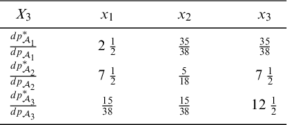
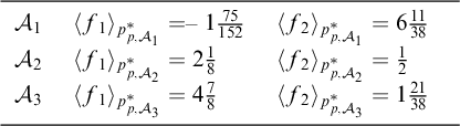
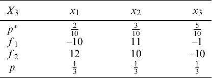

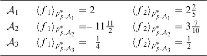
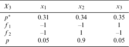

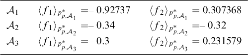
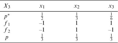
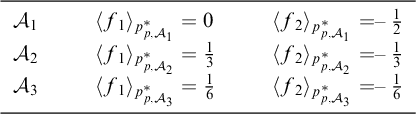


 Open access