Introduction

The short-term flow behaviour of large ice masses can be studied independently of mass and energy considerations, provided that the spatial distribution of material properties and temperature, and basal boundary conditions are known. Owing to the stress-strain-time behaviour of ice, residual stresses are quickly dissipated, unlike with other geologic materials. Consequently, the entire deformation history need not be traced in order to estimate large-scale stress and velocity fields in large ice structures; although it is important to recognize that the flow parameters may change with time due to strain-induced anisotropy (non-random fabric).

During the past several years the finite-element method has received an increase in popularity in glaciology for analysis of two-dimensional glacier flow. This paper extends recent work completed by the author (Reference StolleStolle, 1986) where a zeroth-order stress model is extended and formulated within the framework of the finite-element method, taking into account coupling between stress and displacement fields via an integrated constitutive relationship. The emphasis in this paper is on boundary-valued problem-modelling technique via an integral approach and subsequent simplification, and not on material characterization. It is shown that the simple model presented herein is capable of effecting solutions to glacier-flow problems which are in good agreement with those of two-dimensional finite-element models. In an attempt to simplify the presentation, it is assumed that the ice mass is isothermal and homogeneous, and the ice is isotropic.

Two-Dimensional Finite-Element Models

As indicated previously, during the past several years there has been a move in glaciology toward two-dimensional finite-element modelling of large ice-mass dynamic phenomena, including: creep analysis due to gravity loading (Reference Emery and VoightEmery, 1978; Reference Hooke, Raymond, Hotchkiss and GustafsonHooke and others, 1979; Reference HodgeHodge, 1985; Nguyen, unpublished); thermal analysis (Reference Hooke, Raymond, Hotchkiss and GustafsonHooke and others, 1979); creep and fracture simulation (Chan, unpublished); particle-path determination (Reference Stolle and KilleavyStolle and Killeavy, 1986); and large ice-mass instability (Reference Stolle, Mirza, Selvadurai and VoyiadjisStolle and Mirza, 1986). By no means does this list exhaust all finite-element literature in glaciology. For analysis of flow problems, two distinct approaches have evolved, i.e. initial strain method (DlSP) where the discretized equations are obtained via the principle of virtual work, and the non-Newtonian fluid rheology approach (V—P) where the discretized equations are obtained via the principle of virtual velocities and an incompressibility constraint. The reader is referred to Reference ZienkiewiczZienkiewicz (1977) for details on these approaches.

One-Dimensional Glacier-Flow Model

While the two-dimensional models are useful for giving detailed information on glacier flow, the accuracies provided by these models are often undermined by poor quality of input data. Furthermore, even though good agreement may be obtained when comparing predicted and measured surface velocities, there is generally insufficient data available to confirm agreement of velocities at depth. Thus, the author feels that alternative approaches such as the one presented in the following sections are more appropriate for studying large-scale ice flow.

Constitutive and Sliding Relationships

A large number of creep laws have been proposed for modelling long-term ice creep. Most of these relationships have been developed using uniaxial creep data, and have been extended for multi-axial creep modelling assuming isotropy and ice incompressibility. The power creep law (Reference GlenGlen, 1952) has been adopted for this study due to its ability to predict creep response over the range of stresses typical in glaciers and ice sheets. The law in invariant form is

(1)

where and σ_e are Dorn’s definitions for effective creep strain-rate . and effective stress (σ_e = , respectively. The extension of Equation (1) to multi-axial creep may be written, using index notation, as

(2)

where and S _ij are strain-rate and deviatoric stresses, respectively, and η is the viscosity. Repeated indices where they appear imply summation.

In general the coefficient, A,which depends upon ice temperature and fabric, varies throughout an ice mass. While the approach presented herein can take into account spatial variations in A,it is assumed that Ais constant within each finite element. The exponent n tends to reflect the rate-determining step for the creep process which in turn depends on the stress and temperature levels. For the range of stresses and temperatures which are typical of large ice masses, n = 3 is appropriate (e.g. Reference ColbeckColbeck, 1980).

In order to account for highly concentrated shear near to an ice—bedrock interface due to sliding or presence of warmer and softer ice, the following law has been adopted herein

(3)

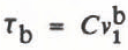
where τ_b and v ₁ ^b are basal shear stress and basal velocity, respectively, C is a function depending on bedrock roughness, properties of ice, and basal velocity (e.g. Reference FowlerFowler, 1979; Reference HutterHutter, 1982).

Kinematics

Fig. 1.

Coordinate system for glacier flow.

Owing to typical ice-sheet and glacier geometries, it may be assumed that , where v ₁, and v ₂. are velocities acting in the x ₁ and x ₂, directions, respectively (see Fig. 1). The notation, i implies differentiation with respect to x _¡. By replacing strain-rate in Equation (2) with rate of deformation , we may write

(4)

In order to allow explicit integration of Equation (4), to obtain the variation of the longitudinal velocity ν ₁, with depth at a certain point above the bedrock, let us follow the approach of Reference Shoemaker and MorlandShoemaker and Morland (1984) and Reference StolleStolle (1986) where variations with depth in S₁₂ and S₁₁ are defined, a priori,as

(5a)

(5b)

where θ represents a dimensionless x ₂-coordinate which ranges from 0 at the bedrock to I at the surface, τ_b is the basal shear stress, S̄ ₁₁ is the average longitudinal deviatoric stress, and mis a parameter which controls the variation of S₁₁ with depth. If appreciable sliding is expected m= 0, otherwise m < 0. It was found in a previous study that, for shear-dominated flow, the surface-velocity and basal shear-stress predictions were not too sensitive to the choice of mFor 0 ≤m<2, horizontal surface-velocity and basal shear-stress predictions varied at most by 10 and 5%, respectively. The variations in the predictions were generally much less (e.g. Reference StolleStolle, 1986).

Integration of Equation (4) subject to Equations (2), (3), and (5) yields

(6a)

with

(6b)

or

(6c)

with

(6d)

where V̄ ₁ is the average longitudinal cross-sectional velocity and Ω(θ) represents an interpolation function for the longitudinal velocity through the depth of the ice mass.

At this point let us briefly examine the influence of C for the two limiting cases of no basal shear resistance, C →0, and the no-slip condition, C →. For the case where C → 0, ν (θ) →ν ₁ ^b and τ_b → 0 which results in the ice weight being fully supported by longitudinal deviatoric stress gradients rather than by shear, as anticipated. For the second case where C → ∞, v ₁ → 0 with remaining finite; that is, the basal shear stress becomes a function of ice-creep properties, ice-mass thickness, and variation in stresses through the depth of the ice mass'. In practice, the no-slip condition can be approximated by selecting a large value for C.

Since the longitudinal velocity also varies along an ice mass, let us further approximate the spatial variation of v ₁ as

(7)

where N _iis a polynomial interpolation function for average longitudinal velocity V̄ ₁ along the ice mass and V̄ _1i . are nodal velocities. The independent variable x ₁ has been included in Ω since ice-mass thickness is a function of x ₁. The vertical velocity v ₂ (x ₁θ) can be obtained by integrating the incompressibility constraint.

The velocity gradients are given by

(8a)

and

(8b)

It should be noted that the first term on the right-hand side of Equation (8a) is generally negligible when compared with the second term, thereby allowing the shown simplification.

Equilibrimn

It has been shown by a number of investigators, owing to the geometry of large ice masses, that plane-strain equilibrium may be approximated as

(9a)

with

(9b)

and

(9c)

where his ice thickness, α_s is surface slope with respect to the horizontal plane, Y is unit weight of ice, and the other terms are the same as defined previously (e.g. Reference ColbeckColbeck, 1980). Assumptions incorporated into the development of Equation (9) include: (a) top surface is traction-free; (b) top and bottom boundaries do not deviate strongly from one another (│α_s — α_b│ << 1); (c) ice is incompressible and isotropic; and (d) density is uniform with depth. For the one-dimensional model presented in this paper (Ф = 0) both α_sand α_b must be small; see Figure 1.

Alternative formulations which improve upon some of the shortcomings of Equation (9) have been suggested, for example, by Reference Shoemaker and MorlandShoemaker and Morland (1984), Reference McMeeking and JohnsonMcMeeking and Johnson (1985), and Reference KambKamb (1986). However, given the previous assumptions, the equations developed by these investigators reduce to Equation (9). Although in recent years use of Equation (9) has been questioned, since proper interactions between flow field, temperature field, and basal boundary conditions may not be properly treated (e.g. Reference Hutter, Legerer and SpringHutter and others, 1981), it will be shown in this paper that use of reduced equations similar to Equation (9) can provide solutions which are in excellent agreement with those obtained using more rigorous two-dimensional finite-element approaches for large-scale isothermal glacier-flow problems.

Reference StolleStolle (1986) used Equation (9) as a starting point to develop its integrated equivalent

(10)

where δV̄ ₁ is a weighting function consistent with the longitudinal variation in average longitudinal velocity V̄ ₁,lis length of ice mass, and the other terms are the same as defined previously. Equation (10) in conjunction with properly vertically averaged constitutive equations as described by Reference Shoemaker and MorlandShoemaker and Morland (1984) or by Reference StolleStolle (1986) was used to formulate a one-dimensional finite-element equivalent of two-dimensional stress equilibrium. The author was able to demonstrate that the one-dimensional model, which he referred to as a two-dimensional line-element model, gives good predictions when compared with those by the more rigorous two-dimensional models, however at much smaller computational and data input efforts. The remainder of this section is used to describe the reduction of the two-dimensional problem to one-dimensional form via the Kantorovich method which makes use of the principle of virtual velocities.

The equilibrium of an ice mass for planar problems can be written in integral form by using the principle of virtual velocities

(11)

where δd _ij is virtual rate of deformation consistent with virtual velocities δv _i,•in x_i ,-direction, b¡are body forces in A,σ_ij are total stresses and i,- are surface tractions on boundary S _t Equation (11) may be used to obtain a one-dimensional equilibrium equation, by enforcing incompressibility exactly, i.e. δd _ii, •= d _ii= 0, and noting that S ₂₂ = -S ₁₁yielding

(12)

The boundary integral term has been omitted since it is not required.

After substitution of Equations (2), (7), and (8) into Equation (12), we have

(13)

The assumptions which are incorporated into the development of Equation (13) are the same as those for the development of Equation (9). The area integrals in Equation (13) can be completed numerically using, for example, Gauss-Quadrature rules. However, it can be shown, for the case of a linear flow law and no basal sliding, that Equation (13) is similar to a simplified form of Equation (10) where the last term containing T,which tends to have negligible influence on predictions (e.g. Reference Kamb and EchelmeyerKamb and Echelmeyer, 1986), is dropped. The stiffness matrix due to the shear contributions is identical for both formulations, with the stiffness due to the longitudinal extension contribution of Equation (13) being stiffer than that of Equation (10) by a factor of 1.2.

This suggests that the influence of weighting through the depth of the ice mass for the non-linear flow-law case can be accounted for in Equation (10), in an approximate manner, by multiplying the first stiffness term of this equation by an appropriate weighting factor F thereby eliminating the need for approximate numerical integration of Equation (13). This factor provides some flexibility in adjusting the stiffness contribution due to longitudinal straining relative to that which is due to shear. Based on a numerical sensitivity study of the ice mass described in the following section for n = 3 and varying C, suitable weighting factors have been found to vary between 1.0 and 1.5. The reader is referred to the Appendix for more details on the matrix formulation used to study the ice mass which is described in the following section.

Numerical Examples

The finite-element models reviewed and described in the previous sections were used to simulate the flow behaviour due to self weight of Barnes Ice Cap, a medium-sized ice cap located on Baffin Island, N.W.T., Canada. The geometry of the ice cap was taken from Reference Hooke, Raymond, Hotchkiss and GustafsonHooke and others (1979); the finite-element grid for the one-dimensional model and geometry are shown in Figure 2. Since this paper emphasizes modelling technique and not material characterization, comparisons between models are made assuming isothermal and homogeneous conditions, and no basal sliding; n= 3, A = 2.2 ×10⁻⁷ (kPa)⁻³ year⁻¹, and Y =8.952 kN/m³ No basal sliding was enforced by specifying a large value for C The solutions of the one-dimensional model (17 elements) are compared with those generated by the displacement (DISP) (372 elements) and non-Newtonian fluid rheology (V—P) (93 elements) approaches. Quadratic element interpolation was incorporated into the one-dimensional and V—P models (e.g. Reference Stolle and KilleavyStolle and Killeavy, 1986), while linear interpolation was used in the DISP model. The one-dimensional simulations were carried out using a TI Professionals microcomputer with 8087 co-processor, while two-dimensional simulations were completed on a VAX-785 minicomputer.

Fig. 2.

Finite-element grid of Barnes Ice Cap for one-dimensional model.

Figures 3, 4, and 5 compare predictions of horizontal surface-velocity, vertical surface-velocity, and basal shear-stress variations along the ice mass, respectively. Two sets of predictions are given using the one-dimensional model. Since the complete velocity field within an element is defined by Equation (6), we can determine S ₁₁variations with depth, thereby allowing us to obtain updated estimates for mwithin each element. However, it was found that updating of mhad negligible influence on predictions and thus a linear variation of S ₁₁ was adopted (m = 1). Solutions effected by the one-dimensional model for this study are given for F = 1.0 and 1.2.

Fig. 3.

Comparison between one- and two-dimensional models of horizontal surface-velocity predictions along Barnes Ice Cap assuming homogeneous isothermal ice mass.

Fig. 4.

Comparison between one- and two-dimensional models of vertical surface-velocity predictions along Barnes Ice Cap assuming homogeneous isothermal ice mass.

Fig. 5.

Comparison between one- and two-dimensional models of basal shear-stress predictions along Barnes Ice Cap assuming homogeneous isothermal ice mass.

Figure 3 demonstrates that the one-dimensional model is capable of providing good predictions when compared with the two-dimensional models. By increasing the factor from 1.0 to 1.2 agreement of horizontal velocities between one-dimensional and V—P is improved, as anticipated. Although not shown, a comparison of stream lines as predicted by V—P (Reference Stolle and KilleavyStolle and Killeavy, 1986) and one-dimensional formulations suggests that the velocity field predicted by each model is similar. The stream-line function Ψ for one-dimensional modelling can be determined by integrating . The differences between DISP and V—P velocity predictions are attributed to the use of lower-order elements for the DISP formulation. This example clearly shows that the one-dimensional approach presented in this paper is capable of yielding better large-scale predictions than two-dimensional finite-element approaches using low-order elements.

A final example is presented where the creep parameter Aalong the ice mass is optimized (see Fig. 6) in order to achieve reasonable agreement between measured and predicted horizontal surface velocities. In a separate unpublished study, the author found, by incorporating the one-dimensional model into a non-linear optimization computer program, that the profile of Barnes Ice Cap investigated in this study must be divided into a minimum of eight regions in order to get reasonable agreement between predicted and measured horizontal surface velocities. Therefore, one flow law cannot be expected to model the stress-strain-rate response through an entire ice mass even if temperature influences are included. Although the most effective way of parameter estimation is via non-linear optimization techniques, these techniques do not always converge or may sometimes converge to an unreasonable solution (e.g. Reference Draper and SmithDraper and Smith, 1966). Owing to the form of Equation (6), optimization in this study was completed by using an iterative procedure where stresses were first estimated using initially assumed Aparameters for the flow analysis, and then the Aparameters in each region were updated using the updated stresses which were obtained by using the predicted velocities from the flow analysis, measured horizontal surface velocities, and Equation (6). This procedure was repeated until reasonable agreement was achieved between measured and predicted surface velocities. While the optimization procedure adopted in this study yielded reasonable Aparameters, the back-calculated solution is by no means considered to be unique.

Fig. 6.

Variation of flow parameter A along Barnes Ice Cap for optimized predictions.

As shown in Figure 2, 17 regions were used for studying Barnes Ice Cap, each having a different Aparameter. The variation in Aparameter, as shown in Figure 6, is attributed to changes in mean temperature and fabric along the ice mass. Although the influence of vertical variation in temperature within each element can be accounted for in the one-dimensional model by introducing a temperature dependency on the Aparameter, it is felt that further improvements in flow modelling are not justified until more field data are available for model calibration. Figure 7 clearly demonstrates that optimization procedures may be used to obtain a reasonable distribution of the Aparameter, which can.lead to good agreement between measured and predicted surface velocities. Based on a recent communication from G. Holdsworth, the measured vertical surface velocities reported in previous publications are 0.206 m a⁻¹ too high (e.g. Reference Hooke, Raymond, Hotchkiss and GustafsonHooke and others 1979; Reference Stolle and KilleavyStolle and Killeavy, 1986). Consequently, the agreement between measured and predicted vertical surface velocities in these publications is better than is reported. The optimized parameters from the one-dimensional model were also used for a V—P simulation. As shown in Figure 7, good agreement was also obtained between the predicted velocities via the V—P model and measured velocities. This suggests that the one-dimensional model can be used to estimate parameters for true two-dimensional analyses.

Fig. 7.

Comparison of measured and predicted (a) horizontal and (b) vertical surface velocities along Barnes Ice Cap using flow-parameter distribution shown in Figure 6.

Closing Remarks

The emphasis in this paper has been on numerical modelling of large ice-mass flow and the reduction of two-dimensional stress equilibrium equations to one-dimensional form via the Kantorovich methodology. In other recent publications addressing one-dimensional modelling (e.g. Reference McMeeking and JohnsonMcMeeking and Johnson, 1985; Reference KambKamb, 1986), the emphasis has tended to be on demonstrating the limits of applicability of the one-dimensional models and the significance of the various terms appearing in, for example, Equation (9). Unlike the integral approach described in this paper, the analysis approach in these (other and related) studies has involved direct use of the differential equations in conjunction with perturbation methods.

It has been demonstrated in this paper that the solutions predicted by relatively simple one-dimensional models compare well with those of two-dimensional models for large-scale flow, provided that integration of constitutive relationships is properly treated. Use of the one-dimensional model allows considerable savings in computational and data-input effort. The value of the approach.presented in this paper lies not so much in reduction of a two-dimensional problem to one-dimensional form for steady-state flow, but for the analysis of long-term transient flow and the reduction of three-dimensional problems to two-dimensional equivalents which will be discussed in a separate paper. Of course, if details of the flow field are important, then full two- or three-dimensional analysis is necessary.

Acknowledgements

The author wishes to express his thanks to M. Killeavy for his assistance in completing numerical simulations, to J. Higgins for aiding preparation of figures, and to G. Holdsworth of Environment Canada for providing field data and its interpretation. The financial support provided by the Natural Sciences and Engineering Research Council of Canada is also appreciated.

Appendix

Summary Of One-Dimensional Model

Substitution of Equation (6) into Equation (9) yields

(A-1a)

Where

(A-1b)

(A-1c)

(A-1d)

with F = 1 and all other terms are the same as defined in the main text. The last term containing T has been assumed negligible.

The factor Fwas introduced into Equation (A-1b) in order to approximate the influence of weighting through the depth of the ice mass as provided for by Equation (13). A standard Choleski procedure for symmetric banded matrices was used to invert the stiffness matrix. Since the ice viscosity is stress-dependent, the direct iteration method was adopted. Convergence in terms of the root-mean-square error of horizontal velocities between two successive iterations being less than 0.1% was achieved within 15 iterations.