


1. Introduction
Financial instability has been a key notion in the macro-finance literature since the pioneering contributions of Kindleberger (Reference Kindleberger1978) and Minsky (Reference Minsky and Minsky1985). Financial instability applies both to the dynamics of financial prices and to the evolution of real activity, that are intertwined and affect each other. In this paper, we focus on one side of financial instability, namely the dynamic pattern of the stock price. The nature of the instability of the stock price has been thoroughly explored in the contemporary finance literature but no overwhelming consensus has been reached. According to the Efficient Market theory (Fama, Reference Fama1991), the oscillating behavior of the stock price (described by a random walk) is triggered by an exogenous shock in an economy characterized by a representative rational agent (Muth, Reference Muth1961). For the behavioral theory (Beja and Goldman, Reference Beja and Goldman1980; Schleifer and Summers, Reference Schleifer and Summers1990; Shiller, Reference Shiller2003; Thaler, Reference Thaler2015; Vikash et al. Reference Vikash, Xiaoming and Imad2015), on the contrary, stock price fluctuations are endogenously determined. In the absence of perfect information, instability emerges from the out-of-equilibrium interaction of investors characterized by bounded rationality. Following the lead of Day and Huang (Reference Day and Huang1990), a sizable number of Heterogeneous Agent Models (HAMs) of the stock market (Chiarella, Reference Chiarella1992; De Grauwe et al. Reference De Grauwe, Dewachter and Embrechts1993; Lux,Reference Lux1995; Brock and Hommes, Reference Brock and Hommes1998; LeBaron, Reference LeBaron2001) to name just a few), focus on behavioral heterogeneity in expectation formation as the driving force of financial instability.Footnote 1
Over the years, this approach has been applied not only to the stock market (Alfarano and Lux, Reference Alfarano and Lux2007; Recchioni et al. Reference Recchioni, Tedeschi and Gallegati2015) but also to the foreign exchange market (De Grauwe and Grimaldi, Reference De Grauwe and Grimaldi2006; Proano, Reference Proano2011; Gori and Ricchiuti, Reference Gori and Ricchiuti2018; Bassi et al. Reference Bassi, Ramos and Lang2023), the housing market (Dieci and Westerhoof, Reference Dieci and Westerhoff2012; Ascari et al. Reference Ascari, Pecora and Spelta2018) and auction markets (Chiarella et al. Reference Chiarella, He and Pellizzari2012). In parallel, empirical methodologies have been developed to investigate the nature of expectations and their potential effects on the financial and economic spheres (for recent surveys, see Lux and Zwinkels, Reference Lux and Zwinkels2018; Ter Ellen and Verschoor, Reference Ter Ellen, Verschoor, Ter Ellen and Verschoor2018). For instance, Franke and Westerhoff (Reference Franke and Westerhoff2017) extract different beliefs from survey evidence. Learning-to-Forecast experiments provide experimental support to the idea that agents follow simple heterogeneous forecasting rules (Anufriev and Hommes, Reference Anufriev and Hommes2012; Colasante et al. Reference Colasante, Alfarano, Camacho and Gallegati2018, Reference Colasante, Alfarano and Camacho-Cuena2019, Reference Colasante, Alfarano, Camacho-Cuena and Gallegati2020a, Reference Colasante, Alfarano and Camacho-Cuena2020b; Bao et al. Reference Bao, Hennequin, Hommes and Massaro2020, Reference Bao, Cars and Jiaoying2021). Along the same lines, direct likelihood or indirect simulated estimation methods can empirically identify different groups of agents (Franke and Westerhoff, Reference Franke and Westerhoff2011; Kukacka and Barunik, Reference Kukacka and Barunik2017; Frijns and Zwinkels, Reference Frijns and Zwinkels2018; Chen and Lux, Reference Chen and Lux2018; Ter Ellen et al. Reference Ter Ellen, Hommes and Zwinkels2021; Lux, Reference Lux2021a; Schmitt, Reference Schmitt2021). This empirical literature supports the view that financial markets are populated by different types of agents, such as speculators who follow destabilizing heuristics (“chartists”) and investors who adopt stabilizing, fundamentals-based strategies (“fundamentalists”).
These heuristics represent latent factors that are not directly observable but are assumed to play a crucial role in shaping observed financial data. Incorporating such factors as unobserved state components in models of financial markets allows researchers to understand the impact of behavioral factors. To the best of our knowledge, Vigfusson (Reference Vigfusson1997) was the first one to employ the Markov regime-switching methodology to explore the dynamics of the foreign exchange market, considering heuristics as distinct states. This approach was subsequently applied to spot and forward exchange rate market (Ahrens and Reitz, Reference Ahrens and Reitz2005; Li et al. Reference Li, Zhou and Wu2013), the stock market (Chiarella et al. Reference Chiarella, He and Pellizzari2012) and the housing market (Chia et al. Reference Chia, Li and Zheng2017). Recently, Lux (Reference Lux2018, Reference Lux2021b) and Majewski et al. (Reference Majewski, Ciliberti and et Bouchaud2020) have advocated the state-space representation of financial markets. In fact, a structural HAM can be reduced to a linear or nonlinear econometric model with latent states. Hence, continuous state-space Markov processes (state-space models for short hereafter) have been explored (Gusella and Stockhammer, Reference Gusella and Stockhammer2021; Gusella, Reference Gusella2022; Gusella and Ricchiuti, Reference Gusella and Ricchiuti2024). As the latent factors can be associated to different beliefs, the state-space methodology is particularly suited to empirically investigate whether these components can generate endogenous dynamical instability in price formation. At the same time, an out-of-sample comparison could help us to understand the power predictability of different notions of instability.
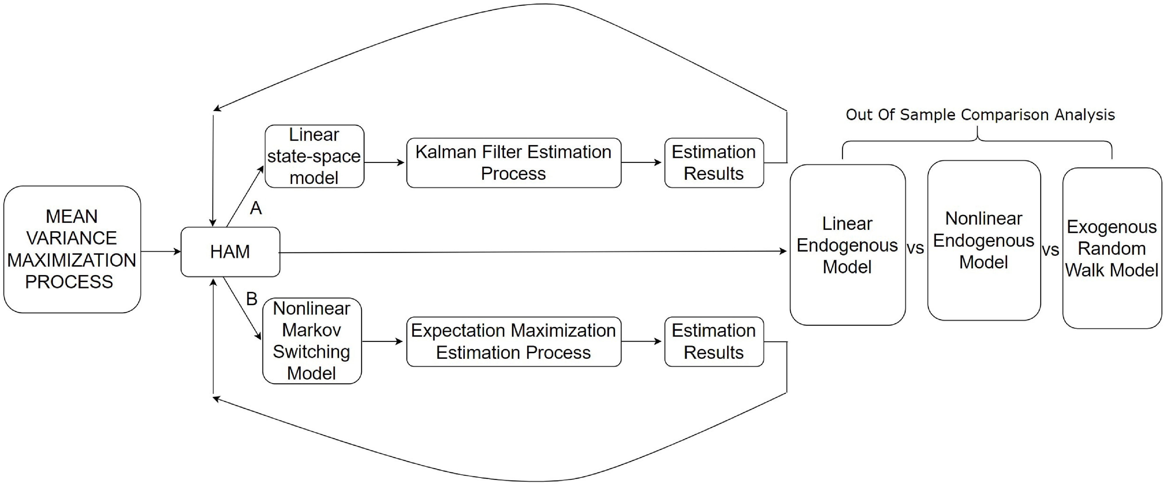
In this paper, we conduct a comprehensive comparison between two frameworks that generate endogenous instability as a consequence of unobserved beliefs – namely (i) a linear state-space model and (ii) a nonlinear Markov-switching process featuring chartists and fundamentalists – and a benchmark random walk model of the stock price, which assumes exogenous fluctuations. This allows us to empirically assess the underlying nature of financial market dynamics. To the best of our knowledge, this is the first attempt in this direction. This empirical assessment allows us to evaluate (i) whether endogenous dynamics provide a better explanation of financial instability than exogenous shocks, and (ii) whether nonlinear, regime-dependent instabilities offer greater explanatory power than linear, globally stable dynamics. In Figure 1 we represent the main steps of our analysis.
Methodology.

We assume that the economy is populated by mean-variance optimizing investors. We construct a conventional HAM wherein agents are classified into two groups: chartists and fundamentalists.Footnote 2 We therefore end up with a 2-type streamlined variant of a standard small-scale dynamic asset pricing model. Since beliefs are latent variables, we first convert the structural theoretical model into a reduced linear state-space form (path A). In the state-space model, we distinguish between observed and unobserved variables. In our case, the asset price will be the observed variable. In contrast, the beliefs of the agentsFootnote 3 will be the unobserved components that dynamically influence the observation value over time. In this way, we can detect endogeneity that comes from the heuristics of the agents. In fact, we are able to study the mathematical conditions to obtain complex endogenous dynamics; analytical results confirm that these conditions are restrictions on the parameter associated with the group of trend followers.
Our approach so far departs from Gusella and Stockhammer (Reference Gusella and Stockhammer2021) and Gusella (Reference Gusella2022) because in the present paper agents’ strategies are unobservable. This enables us to uncover hidden heuristics and grasp their dynamic impact on the observable asset price, with a specific emphasis on oscillatory dynamics. Moreover, we introduce different heuristics and specify the fundamental asset price as an exogenous value and not as an unobservable variable. In fact, fundamentalists base their expectations on the deviations between observed fundamental values and market prices, expecting these to converge. Compared to Lux (Reference Lux2018, Reference Lux2021b), we work with a frequentist approach and consider the strategies adopted by the agents as unobservable. Differently from Majewski et al. (Reference Majewski, Ciliberti and et Bouchaud2020), the fundamental value is constructed from the observed data.
To address the unrealistic assumption of exogenous composition of the population of investors in Gusella and Ricchiuti (Reference Gusella and Ricchiuti2024), in the present paper we introduce a nonlinear two-state Markov switching model (path B) in which the latent shares of fundamentalists and chartists evolve over time. Indeed, in the real world investors are likely to switch from one strategy to another on the basis of the relative performance of each heuristic (for instance, in predicting the stock price). When the fundamentalist regime prevails, asset price dynamics are primarily driven by changes in the fundamental value. Conversely, when the trend-following regime dominates, the current price is influenced predominantly by its own past values. The probability of being in either regime serves as a proxy for the weight assigned to the corresponding heuristic. Although different groups of agents form expectations using different rules, the auctioneer sets the market-clearing price as a weighted average of their forecasts. This weighting is dynamically determined by the time-varying probabilities associated with the latent regime states. Unlike Vigfusson (Reference Vigfusson1997), Ahrens and Reitz (Reference Ahrens and Reitz2005), Li et al. (Reference Li, Zhou and Wu2013) and Chia et al. (Reference Chia, Li and Zheng2017) we incorporate regime-switching models into equity prices, as done by Chiarella et al. (Reference Chiarella, He and Pellizzari2012). Unlike Chiarella et al. (Reference Chiarella, He and Pellizzari2012), the switching process involves regime changes for both speculative strategies, not just within a single group. For both specifications, we perform Monte Carlo maximum likelihood estimation analysis. In the first case, we use the Kalman filter to recover the log-likelihood function and the parameters associated to the beliefs of the agents. In the second case, we use the Expectation-Maximization algorithm to optimize the data likelihood.
Finally, we contribute to the existing literature on HAMs that incorporate unobserved components in the state-space framework by comparing the linear (c&f)Footnote 4 model, the nonlinear (c&f) switching model, and the benchmark random walk model with each other. Lux (Reference Lux2021a) carried out a similar comparison but within an in-sample context of latent variables. We move a step further, comparing the three specifications in a rolling window state-space out-of-sample forecasting context. This comparison allows to detect which type of specification increases the forecasting performance of the model.
Analyzing the S&P 500 data on a time window ranging from 1990 to 2019 at monthly frequency, we find evidence of endogenous fluctuations. Furthermore, covering an out-of-sample evaluation period from January 2017 to December 2019, this study suggests that including behavioral non-linearity improves the model’s predictability in the short, medium and long run over the linear behavioral model and the benchmark random walk hypothesis.
The remainder of the paper is structured as follows. Section 2 introduces the model, beginning with the construction of the heterogeneous agent framework (Section 2.1), which is then reformulated as a linear state-space representation (Section 2.2), where we also derive the analytical conditions for the emergence of endogenous cycles. Section 2.3 extends the model to a nonlinear Markov regime-switching framework. Section 3 presents the Monte Carlo estimation results, while Section 4 provides the rolling-window out-of-sample forecasting analysis used to compare the three model specifications. Section 5 concludes.
2. The model
2.1. General set-up
In line with Brock and Hommes (Reference Brock and Hommes1997, Reference Brock and Hommes1998) and Hommes (Reference Hommes2005), financial operators at time
 $t$
can invest in two asset types - a risk-free asset offering a fixed rate of return
$t$
can invest in two asset types - a risk-free asset offering a fixed rate of return
 $r$
and a risky asset with price
$r$
and a risky asset with price
 $p$
and a stochastic dividend
$p$
and a stochastic dividend
 $y$
. The dynamics of wealth at the end of period
$y$
. The dynamics of wealth at the end of period
 $t+1$
can be captured by the following dynamic equation:
$t+1$
can be captured by the following dynamic equation:
 \begin{equation*}W_{t + 1} = (1 + r)W_t + \left [ {{p_{t + 1}} + {y_{t + 1}} - (1 + r){p_t}} \right ]z_t,\end{equation*}
where
 $W$
indicates the end-of-period wealth while
$W$
indicates the end-of-period wealth while
 $z$
is the number of shares of the risky asset purchased at date
$z$
is the number of shares of the risky asset purchased at date
 $t$
. Agents are assumed to be mean-variance maximizer, such that:
$t$
. Agents are assumed to be mean-variance maximizer, such that:
 \begin{equation*}{\max _{zt}}\left \{ {{E_t^i}\left [ {{W_{t + 1}}} \right ] - \frac {a}{2}{\sigma ^2}} \right \},\end{equation*}
where
 $E_t^i$
is the expectation operator of agents of type
$E_t^i$
is the expectation operator of agents of type
 $i$
,
$i$
,
 $\sigma ^2$
is the conditional variance of the wealth, supposed to be constant over time and equal for all types of agents, and
$\sigma ^2$
is the conditional variance of the wealth, supposed to be constant over time and equal for all types of agents, and
 $a\gt 0$
represents the risk aversion parameter. Maximizing with respect the demand
$a\gt 0$
represents the risk aversion parameter. Maximizing with respect the demand
 $z_t$
by trader type
$z_t$
by trader type
 $i$
, we obtain:
$i$
, we obtain:
 \begin{equation*}z_t^i = \frac {{E_t^i( {{p_{t + 1}}}) + \bar y - (1 + r){p_t}}}{{a\sigma ^2}},\end{equation*}
where expectations regarding dividends are uniform across all trader types and equal to the conditional expectation
 $\bar y$
.
$\bar y$
.
Suppose now there are
 $I$
groups of investors, each with diverse expectations regarding the future price
$I$
groups of investors, each with diverse expectations regarding the future price
 $p_{t+1}$
. We assume that
$p_{t+1}$
. We assume that
 $\delta ^i$
is the fraction (market share) of type
$\delta ^i$
is the fraction (market share) of type
 $i$
investors, with
$i$
investors, with
 $\sum \nolimits _{i = 1}^I {{\delta _i}} = 1$
. From the equilibrium between the total demand for the risky asset and the supply side supposed to be equal to zero, we get:
$\sum \nolimits _{i = 1}^I {{\delta _i}} = 1$
. From the equilibrium between the total demand for the risky asset and the supply side supposed to be equal to zero, we get:
 \begin{equation*}(1 + r){p_t} = \sum \limits _i^I {\delta ^iE_t^i( {{p_{t + 1}}})} + \bar y.\end{equation*}
Consistent with HAMs, the heterogeneity of agents is attributed to their distinct methods of expectation formation. Specifically, financial traders employ either a fundamental or a technical expectation rule to project future prices. Thereby:
 \begin{equation*}(1 + r){p_t} = \delta E_t^f( {{p_{t + 1}}}) + ( {1 - \delta })E_t^c( {{p_{t + 1}}}) + \bar y.\end{equation*}
where
 $E_t^f$
and
$E_t^f$
and
 $E_t^c$
are the expectation operators of fundamentalists and chartists, respectively.
$E_t^c$
are the expectation operators of fundamentalists and chartists, respectively.
Under the assumption that both the risk-free rate and the constant dividend are equal to zero, the price of the risky asset is expressed as follows:
 \begin{equation} {p_t} = \delta E_t^f( {{p_{t + 1}}}) + ( {1 - \delta })E_t^c( {{p_{t + 1}}}). \end{equation}
We now formalize the expectation formation of the two groups of agents considered. Fundamentalists believe in the efficient market theory, expecting the price to be equal to the fundamental value
 $p_t^f$
:
$p_t^f$
:
 \begin{equation} E_t^f( {{p_{t + 1}}}) = p_{t}^f. \end{equation}
Conversely, the expectation for chartists is expressed as follows:
 \begin{equation} E_t^c( {{p_{t + 1}}}) = p_{t}^f + \beta ( {{p_{t - 1}} - {p_{t - 2}}}),\quad \quad \textrm{with}\quad \beta \gt 0 \end{equation}
where parameter
 $\beta$
represents the reaction coefficient, indicating the degree to which speculators extrapolate past changes in the asset market. At this point two important remarks are in order. First, in our setting fundamentalists are “dogmatic” since they expect the stock price to revert to the fundamental value in one period (Levy, Reference Levy2010; Franke, Reference Franke2008). This assumption makes the transformation of the theoretical model into a state-space form feasible, avoiding multiple solutions for
$\beta$
represents the reaction coefficient, indicating the degree to which speculators extrapolate past changes in the asset market. At this point two important remarks are in order. First, in our setting fundamentalists are “dogmatic” since they expect the stock price to revert to the fundamental value in one period (Levy, Reference Levy2010; Franke, Reference Franke2008). This assumption makes the transformation of the theoretical model into a state-space form feasible, avoiding multiple solutions for
 $\beta$
, the reaction parameter of chartists.Footnote
5
Second, following the modeling strategy of (a part of) the theoretical literature on behavioral models of the stock market with different types of expectational heuristics, we assume that chartists incorporate the fundamental value of the stock price in their expectations (together with past prices). In this literature, in fact, expectations are decomposed into a base price – that is uniform across types – and a Belief function that describes the way in which agents of each type form their beliefs. The base price may be the current market price, the lagged price or the fundamental price. When the base price is the fundamental price, chartists share with fundamentalists the conviction that the stock price will tend over the long run to the fundamental value (Franke Reference Franke2008, p. 12).
$\beta$
, the reaction parameter of chartists.Footnote
5
Second, following the modeling strategy of (a part of) the theoretical literature on behavioral models of the stock market with different types of expectational heuristics, we assume that chartists incorporate the fundamental value of the stock price in their expectations (together with past prices). In this literature, in fact, expectations are decomposed into a base price – that is uniform across types – and a Belief function that describes the way in which agents of each type form their beliefs. The base price may be the current market price, the lagged price or the fundamental price. When the base price is the fundamental price, chartists share with fundamentalists the conviction that the stock price will tend over the long run to the fundamental value (Franke Reference Franke2008, p. 12).
Notice moreover that equation (3) can be interpreted as a special case of the so-called First Order Heuristic (FOH) put forward by Heemeijer et al. (Reference Heemeijer, Hommes, Sonnemans and Tuinstra2009) to interpret the forecasting behavior of human subjects in Learning to Forecast (LtF) laboratory experiments. The FOH is an anchoring and adjustment heuristic, i.e., a combination of an anchor and a trend-extrapolating term proportional to the lagged first difference of the variable. Experimental evidence shows that the majority of participants in LtF experiments use variants of this heuristic. In equation (3) the anchor is the long run (fundamental) value and the trend-extrapolating term is the usual one.Footnote 6
Last but not least, this assumption allows to derive the state vector of the agents’ beliefs as a function of unobserved variables only. If the base price were the lagged current price, in fact, agents’ beliefs would be functions of observed (and unobserved) variables, which contradicts the logic of state-space models.
Substituting equations. (2) and (3) in equation (1), we obtain:
 \begin{equation*}{p_t} = \delta \big( {p_{t}^f } \big) + ( {1 - \delta })\Big( {p_{t}^f + \beta ( {{p_{t - 1}} - {p_{t - 2}}})} \Big),\end{equation*}
from which:
 \begin{equation*}{p_t} = p_{t}^f + ( {1 - \delta })\beta ( {{p_{t - 1}} - {p_{t - 2}}}).\end{equation*}
With respect to the belief of chartists, this last equation can be rewritten in the following way:
 \begin{equation} {p_t} = p_t^f + ( {1 - \delta })B_t^c, \end{equation}
with:
 \begin{equation*}B_t^c = \beta ( {{p_{t - 1}} - {p_{t - 2}}}).\end{equation*}
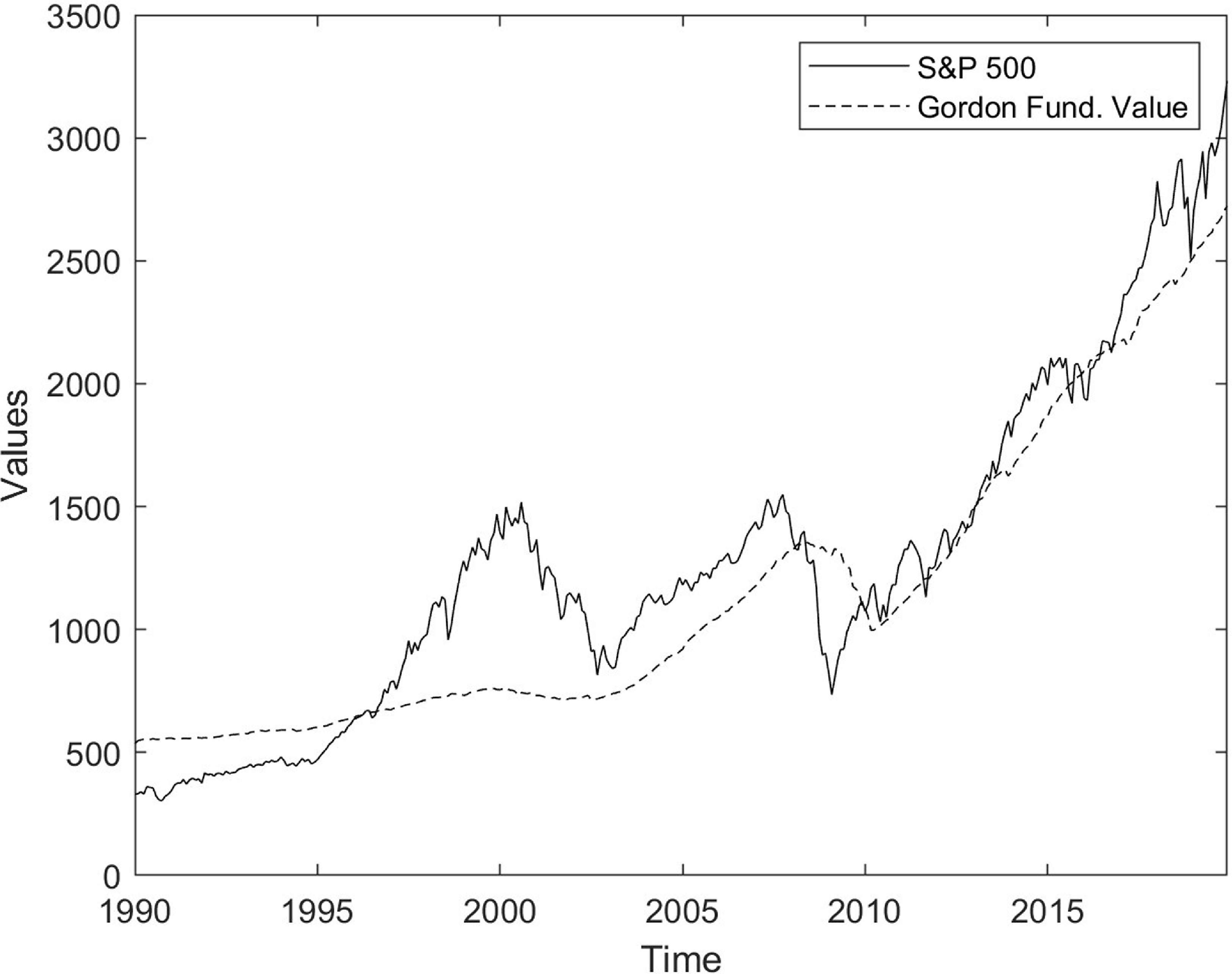
Finally, for the construction of the fundamental value, we derive it from the Gordon growth model (Gordon, Reference Gordon1959) using S&P500 data on dividends. Defining
 $\tilde g$
as the average growth rate of dividends,
$\tilde g$
as the average growth rate of dividends,
 $\tilde r$
the average required return, and
$\tilde r$
the average required return, and
 $d_t$
the dividend flow, the fundamental value of asset price can be defined as:
$d_t$
the dividend flow, the fundamental value of asset price can be defined as:
 \begin{equation*}p_t^f = {d_t}\frac {{( {1 + \tilde g})}}{{\left ( {\tilde r - \tilde g} \right )}}.\end{equation*}
Following Chiarella et al. (Reference Chiarella, He and Pellizzari2012), we assume that
 $\tilde r$
is equal to the sum of the average dividend yield
$\tilde r$
is equal to the sum of the average dividend yield
 $\tilde y$
and the average rate of capital gain
$\tilde y$
and the average rate of capital gain
 $\tilde x$
. The Gordon growth model implies that
$\tilde x$
. The Gordon growth model implies that
 $\tilde x$
is equal to
$\tilde x$
is equal to
 $\tilde g$
, so as to obtain:
$\tilde g$
, so as to obtain:
 \begin{equation*}p_t^f = {d_t}\frac {{( {1 + \tilde g})}}{{\tilde y}}.\end{equation*}
2.2. Linear state-space form
To convert the structural theoretical model of Section 2.1 in a reduced state-space form, equation (4) is substituted in the belief function of chartists, so as to obtain:
 \begin{equation*}B_t^c = \beta \left ( {p_{t - 1}^f + ( {1 - \delta })B_{t - 1}^c - p_{t - 2}^f - ( {1 - \delta })B_{t - 2}^c} \right ).\end{equation*}
Following Franke (Reference Franke2008) and Lux (Reference Lux2021a), we assume that the logarithm of the fundamental value follows a random walk with a normally distributed disturbance term, zero mean, and constant variance. The assumption of unit root is empirically tested using an augmented Dickey–Fuller test on the Gordon-based fundamental price series, and the results fail to reject the null hypothesis.Footnote 7 We thus have:
 \begin{equation*}B_t^c = \beta ( {1 - \delta })B_{t - 1}^c - \beta ( {1 - \delta })B_{t - 2}^c + \varepsilon _t.\end{equation*}
In a matrix-vector formulation, the state-space form assumes the following form:
 \begin{align}&\qquad\qquad\quad {p_t} = p_t^f + \left [ ( {1 - \delta }) \quad 0 \right ]\left [ {\begin{array}{*{20}{c}} {B_{t }^c}\\ {B_{t - 1}^c} \end{array}} \right ] \end{align}
 \begin{align}& \left [ {\begin{array}{*{20}{c}} {B_{t }^c}\\ {B_{t - 1}^c} \end{array}} \right ] = \left ( {\begin{array}{*{20}{c}} {\beta ( {1 - \delta })}&\quad{ - \beta ( {1 - \delta })}\\ 1&\quad 0 \end{array}} \right )\left [ {\begin{array}{*{20}{c}} {B_{t - 1}^c}\\ {B_{t - 2}^c} \end{array}} \right ] + \left [ {\begin{array}{*{20}{c}} {{\varepsilon _t}}\\ 0 \end{array}} \right ]_. \end{align}
The measurement equation is represented by equation (5), whereas the unobserved state equation, containing the belief function of chartists, is depicted by equation (6). As formalized in our model, the belief function impacts price dynamics, thereby potentially inducing endogenous instability in the form of fluctuations. The dynamics, fully expressed by the eigenvalues associated with the transition matrix, can be studied by solving for the determinant of the characteristic equation:
 \begin{equation*}\det \left ( {\begin{array}{*{20}{c}} {\beta ( {1 - \delta }) - \lambda }&\quad{ - \beta ( {1 - \delta })}\\ 1&\quad{ - \lambda } \end{array}} \right ) = 0.\end{equation*}
Once the determinant of the characteristic equation is obtained, the condition to obtain endogenous fluctuations is reflected in complex eigenvalues if the following condition on the discriminant is satisfied:
 \begin{equation*}\Delta =\beta ( {1 - \delta })\left [ {\beta ( {1 - \delta }) - 4} \right ] \lt 0,\end{equation*}
i.e., as a sufficient and necessary condition:
 \begin{equation} 0\lt \beta ( {1 - \delta }) \lt 4. \end{equation}
From the last equation, it is crucial to have a certain percentage of chartists in the market and a positive reaction parameter. If either
 $\beta$
or
$\beta$
or
 $1-\delta$
are equal to zero, the market price will reflect the fundamental price, aligning with the efficient market hypothesis.
$1-\delta$
are equal to zero, the market price will reflect the fundamental price, aligning with the efficient market hypothesis.
If condition in equation (7) holds, the eigenvalues assume the following form:
 \begin{equation*}{\lambda _{1,2}} = \frac {{\beta ( {1 - \delta })}}{2} \pm i\frac {{\sqrt { - \Delta } }}{2} = a \pm ib,\end{equation*}
or in an equivalent trigonometric form:
 \begin{equation*}{\lambda _{1,2}} = \rho \left ( {\cos \theta \pm \sin \theta } \right )\quad {\rm with}\quad \rho = {\left ( {{a^2} + {b^2}} \right )^{1/2}}.\end{equation*}
If complex dynamics is satisfied and
 $\rho =\sqrt {\beta ( {1 - \delta })} = 1$
, we obtain constant endogenous fluctuations. If
$\rho =\sqrt {\beta ( {1 - \delta })} = 1$
, we obtain constant endogenous fluctuations. If
 $\rho =\sqrt {\beta ( {1 - \delta })} \lt 1$
, we observe damped endogenous fluctuations, while explosive endogenous fluctuations if
$\rho =\sqrt {\beta ( {1 - \delta })} \lt 1$
, we observe damped endogenous fluctuations, while explosive endogenous fluctuations if
 $\rho =\sqrt {\beta ( {1 - \delta })} \gt 1$
.
$\rho =\sqrt {\beta ( {1 - \delta })} \gt 1$
.
To simplify the notation, we define
 $a_{11}$
as
$a_{11}$
as
 $\beta ( {1 - \delta })$
and
$\beta ( {1 - \delta })$
and
 $a_{12}$
as
$a_{12}$
as
 $- \beta ( {1 - \delta })$
. Thus, the state-space model takes the following form:
$- \beta ( {1 - \delta })$
. Thus, the state-space model takes the following form:
 \begin{equation*}{p_t} = p_t^f + H{B_t}\end{equation*}
 \begin{equation*}{B_t} = A{B_{t - 1}} + \varphi _t \quad \quad {\varphi _t} \sim \textrm { N} \left ( {0,Q} \right ). \end{equation*}
where
 $p_t$
is the observable asset price,
$p_t$
is the observable asset price,
 \begin{equation*}{B_t} = \left [ {\begin{array}{*{20}{c}} {B_{t }^c}\\ {B_{t - 1}^c} \end{array}} \right ]\end{equation*}
is the state vector,
 \begin{equation*}H = \left [( {1 - \delta })\quad 0 \right ]\end{equation*}
is the measurement matrix,
 \begin{equation} A = {\left ( {\begin{array}{c@{\quad}c} {{a_{11}}}&{{a_{12}}}\\ 1&0 \end{array}} \right )_,}\quad \textrm{with}\quad \left \{ \begin{array}{l} {a_{11}} = ( {1 - \delta })\beta \\ {a_{12}} = - ( {1 - \delta })\beta \end{array} \right . \end{equation}
is the transition matrix and
 $\varphi _t$
is the vector containing the state disturbance of the unobserved component, normally distributed with mean zero and variances collected in the diagonal matrix
$\varphi _t$
is the vector containing the state disturbance of the unobserved component, normally distributed with mean zero and variances collected in the diagonal matrix
 $Q$
.
$Q$
.
2.3. Nonlinear Markov regime-switching form
The linear formalization of the previous section has a potential shortcoming. In fact, agents can switch between the two strategies during different phase of time. To capture this feature, the previous framework is enriched with a nonlinear two-states Markov switching mechanism.
Since we consider two groups of agents with different expectations that influence price dynamics, we can consider the system in two different regimes (or states): the speculative and the fundamentalist regime. Each regime forms two submodels. In one regime, the fundamentalists dominate the market and the dynamics of the price should be reflected by the variation of fundamental price. In the second regime, speculative strategies dominate the market and the unobserved submodel is driven by an autoregressive process. The switching mechanism is controlled by an unobservable state variable that follows a first-order Markov chain. Thus, a specific behavioral rule (for example, the fundamentalists’ behavior) only prevails for a specific time, after which it can possible ”switch” to another behavioral rule (the chartists’ behavior).
Empirically, to study the dynamic behavior of asset price in each regime, we implement a Markov-switching dynamic regression (MSDR) model (Hamilton, Reference Hamilton1994; 2016). Considering the first difference for asset price leads to the following equation:Footnote 8
 \begin{equation*}{p_t} - {p_{t - 1}} = \Big( {p_t^f - p_{t - 1}^f} \Big) + (1 - \delta ) \beta ( {{p_{t - 1}} - {p_{t - 2}}}) - (1- \delta ) \beta ( {{p_{t - 2}} - {p_{t - 3}}}).\end{equation*}
Such that, with
 ${a_{11}} = (1 - \delta )\beta$
,
${a_{11}} = (1 - \delta )\beta$
,
 ${a_{12}} =- (1 - \delta )\beta$
and the Brownian motion for the fundamental value, we obtain:
${a_{12}} =- (1 - \delta )\beta$
and the Brownian motion for the fundamental value, we obtain:
 \begin{equation*}{p_t} - {p_{t - 1}} = {\varepsilon _t} + {a_{11}}( {{p_{t - 1}} - {p_{t - 2}}}) + {a_{12}}( {{p_{t - 2}} - {p_{t - 3}}}),\end{equation*}
from which:
 \begin{equation*}{p_t} - {p_{t - 1}} = {\varepsilon _t}( {{s_t}}) + [ {{a_{11}}( {{p_{t - 1}} - {p_{t - 2}}}) + {a_{12}}( {{p_{t - 2}} - {p_{t - 3}}})} ]( {{s_t}}).\end{equation*}
with:
 \begin{equation*}{p_t} - {p_{t - 1}} = \left \{ \begin{array}{l} fundamentalist\ regime\quad if\;s_t = f\\ chartists\ regime\quad \quad \quad \;\;\,\;\,if\;s_t = c \end{array} \right .\end{equation*}
where
 $s_t$
is the latent state-space discrete-time Markov chain representing the switching mechanism among the two regimes.
$s_t$
is the latent state-space discrete-time Markov chain representing the switching mechanism among the two regimes.
There are four kinds of state transitions possible between the two states:
-
• From state
 $f$
to state
$f$
: This transition happens with probability
${p_{ff}} = P( {{s_t} = f | {{s_{t - 1}} = f}} )$
Footnote
9
$f$
to state
$f$
: This transition happens with probability
${p_{ff}} = P( {{s_t} = f | {{s_{t - 1}} = f}} )$
Footnote
9
-
• From state
$f$
to state
$c$
: This transition happens with probability
${p_{fc}} = P( {{s_t} = c | {{s_{t - 1}} = f}} )$
-
• From state
$c$
to state
$f$
: This transition happens with probability
${p_{cf}} = P( {{s_t} = f | {{s_{t - 1}} = c}} )$
-
• From state
$c$
to state
$c$
: This transition happens with probability
${p_{cc}} = P( {{s_t} = c | {{s_{t - 1}} = c}} )$


with:
 \begin{equation*}{p_{ff}} + {p_{fc}} = 1\quad \textrm{and}\quad {p_{cf}} + {p_{cc}} = 1.\end{equation*}
In the end,
 $s_t$
depends on
$s_t$
depends on
 $s_{t-1}$
according to the following state transition matrix:
$s_{t-1}$
according to the following state transition matrix:
 \begin{equation*}\left [ {\begin{array}{c@{\quad}c} {{p_{ff}}}&{{p_{fc}}}\\ {{p_{cf}}}&{{p_{cc}}} \end{array}} \right ]_.\end{equation*}
This extension, with the filtering process of the unobserved latent states, offers valuable insights into how different market strategies prevail during crucial periods, helping us to better understand the local dynamics of financial markets.
3. In sample estimation results
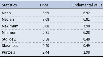
Once the structural model has been transformed into reduced form for the estimation process, we estimate both the linear and nonlinear version with the S&P 500 data using the closing adjusted values from January 1990 to December 2019 at monthly frequency (Figure 2).Footnote 10 For the econometric analysis, all the series are transformed in log levels. Table 1 shows the summary statistics for both the realized (log) market prices and the constructed (log) fundamental price. The mean and median of both series are quite close, suggesting approximate symmetry, although the skewness values reveal some notable differences. The asset price distribution exhibits negative skewness (−0.40), indicating a slight asymmetry with a longer left tail – implying that larger-than-usual drops in price are more likely than extreme increases. In contrast, the fundamental value is positively skewed (0.49), suggesting a tendency for the distribution to be pulled toward higher values. This asymmetry might reflect occasional spikes in dividend-driven fundamentals, whereas market prices may be more prone to sharp downturns, possibly due to speculative episodes or behavioral overreactions.
Descriptive statistics

Market and fundamental price.

For the linear model, we utilize the recursive Kalman filter algorithm to determine the optimal estimator for the state variable and to estimate the parameters via the maximum likelihood function (see Durbin and Koopman, Reference Durbin and Koopman2012; Enders, Reference Enders2016). The prediction error decomposition process involves iterative computation based on one-step prediction and updating equations over the state-space form to estimate
 $a_{11}$
and
$a_{11}$
and
 $a_{12}$
as well as the percentage of chartists in the market
$a_{12}$
as well as the percentage of chartists in the market
 $(1 - \delta )$
.Footnote
11
The procedure is implemented through 1,000 Monte Carlo repetitions. Specifically, we simulate 1,000 sample paths from the estimated model by drawing state disturbances from a standard normal distribution and incorporating them into the state-space framework. The estimation process is repeated for each simulated path.Footnote
12
Based on Monte Carlo estimations, we verify whether the condition for endogenous fluctuation phenomena holds
$(1 - \delta )$
.Footnote
11
The procedure is implemented through 1,000 Monte Carlo repetitions. Specifically, we simulate 1,000 sample paths from the estimated model by drawing state disturbances from a standard normal distribution and incorporating them into the state-space framework. The estimation process is repeated for each simulated path.Footnote
12
Based on Monte Carlo estimations, we verify whether the condition for endogenous fluctuation phenomena holds
 $\left \{ {\beta ( {1 - \delta })\left [ {\beta ( {1 - \delta }) - 4} \right ] \lt 0} \right \}$
. Throughout the estimation process, we assume the percentage of chartists in the market between zero and one. Additionally, we enforce the equality constraint
$\left \{ {\beta ( {1 - \delta })\left [ {\beta ( {1 - \delta }) - 4} \right ] \lt 0} \right \}$
. Throughout the estimation process, we assume the percentage of chartists in the market between zero and one. Additionally, we enforce the equality constraint
 ${a_{11}} + {a_{12}} = \beta ( {1 - \delta }) - \beta ( {1 - \delta }) = 0$
to ensure a unique positive reaction coefficient
${a_{11}} + {a_{12}} = \beta ( {1 - \delta }) - \beta ( {1 - \delta }) = 0$
to ensure a unique positive reaction coefficient
 $\beta$
retrieved from system 8.
$\beta$
retrieved from system 8.
Differently from the linear case, Markov switching estimation is performed using the Expectation Maximization algorithm following the method developed for time series analysis by Hamilton (Reference Hamilton1994, Reference Hamilton and Hamilton2016). The EM iteration involves an expectation (E) step and a maximization (M) step. During the expectation step, the algorithm computes the expected values of latent variables given the current parameter estimates. Subsequently, the maximization step computes parameter values that maximize the anticipated log-likelihood obtained from the E step. These estimated parameters are then employed to recover the distribution of latent variables in the subsequent E step.Footnote 13 As before, estimates are based on 1000 Monte Carlo randomly generated inputs.
The empirical results are divided into two main subsection. In the first, we present results from the linear state-space model. In the second subsection, we present the results of the nonlinear Markov model.
3.1. Linear behavioral model
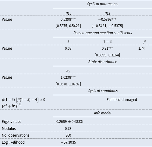
Table 2 presents Monte Carlo results obtained from estimating the model in a linear state-space form. The table is organized in 3 blocks. The uppermost part displays coefficients for the cyclical parameters, followed by the values of the percentage and reaction coefficient of chartists in the second row, along with the associated value for the state disturbance in the third row. The middle block provides information about the endogenous cycles. The bottom part of the table includes general estimation information.
Monte Carlo results [state-space model]

Notes: Confidence interval in squared brackets.
 $^{*}$
,
$^{*}$
,
 $^{**}$
,
$^{**}$
,
 $^{***}$
denotes statistical significance at the 10, 5, and 1% levels respectively.
$^{***}$
denotes statistical significance at the 10, 5, and 1% levels respectively.
We focus on the cyclical parameters of the transition matrix. Our findings from the linear state-space model suggest that cyclical conditions are respected in the necessary and sufficient conditions
 $\left \{ {\beta ( {1 - \delta })\left [ {\beta ( {1 - \delta }) - 4} \right ] \lt 0} \right \}$
. In particular, the coefficients
$\left \{ {\beta ( {1 - \delta })\left [ {\beta ( {1 - \delta }) - 4} \right ] \lt 0} \right \}$
. In particular, the coefficients
 $a_{12}= 0.5398$
and
$a_{12}= 0.5398$
and
 $a_{21}= -0.5398$
are statistically significant at one percent, confirming the nature of complex eigenvalues. The existence of complex eigenvalues underscores how price dynamics reflects endogenous fluctuation phenomena, characterized by dampened fluctuations with a modulus equal to 0.73
$a_{21}= -0.5398$
are statistically significant at one percent, confirming the nature of complex eigenvalues. The existence of complex eigenvalues underscores how price dynamics reflects endogenous fluctuation phenomena, characterized by dampened fluctuations with a modulus equal to 0.73
 $[\sqrt {\beta ( {1 - \delta })} \lt 1]$
.
$[\sqrt {\beta ( {1 - \delta })} \lt 1]$
.
The estimated percentage of trend followers in the market is
 $1-\delta =0.31$
, indicating that they are in the minority compared to agents who follow fundamentalist behavior (
$1-\delta =0.31$
, indicating that they are in the minority compared to agents who follow fundamentalist behavior (
 $\delta =0.69$
) with a reaction coefficient of
$\delta =0.69$
) with a reaction coefficient of
 $\beta =1.74$
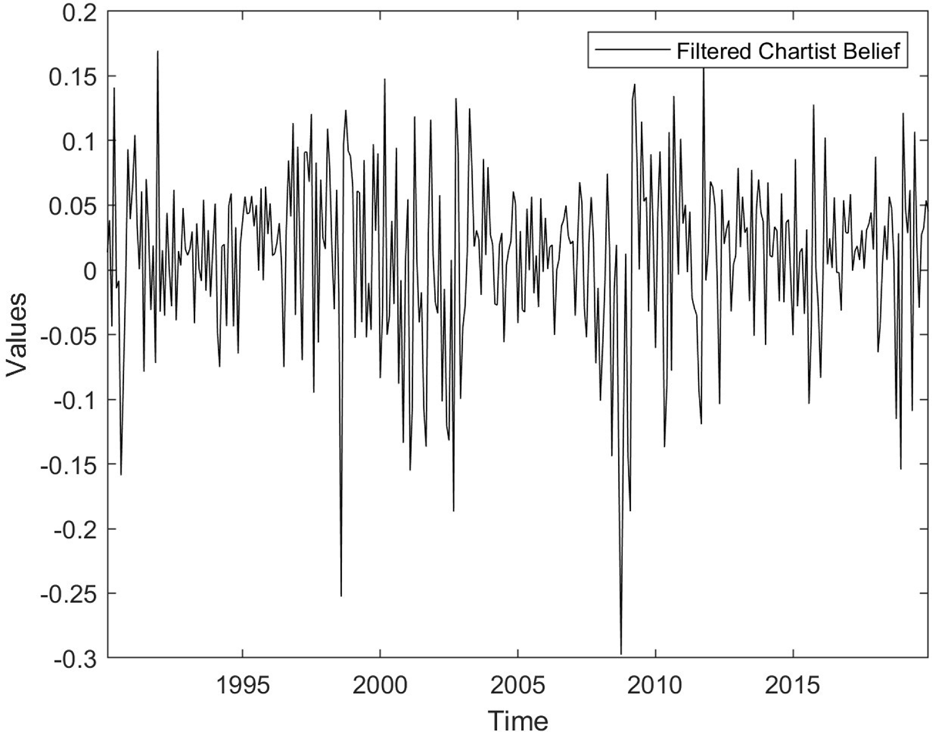
. Figure 3 shows the filtered beliefs of the chartists over the sample period. Detecting the magnitude and direction of the chartist’s belief, we can observe positive signs during the boom phase which turn negative during downturns, with a sharp downward spike after the explosion of the global financial crisis.
$\beta =1.74$
. Figure 3 shows the filtered beliefs of the chartists over the sample period. Detecting the magnitude and direction of the chartist’s belief, we can observe positive signs during the boom phase which turn negative during downturns, with a sharp downward spike after the explosion of the global financial crisis.
To summarize, our results align with HAMs tradition, which documents the presence of different agents in the market with different beliefs. In addition, with the state-space analysis, we document the crucial effect of heuristics in the determination of price dynamics, thereby supporting the hypothesis that endogenous cyclical conditions can arise from the speculative positions taken by agents and formalized in our theoretical model.
Filtered unobserved belief of chartists.

3.2. Nonlinear behavioral model
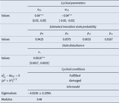
We now present the results obtained from the nonlinear specification. Table 3 is divided into three main blocks. Similarly to the previous table, at the top of the table, the first row displays coefficients for the cyclical parameters. The second row indicates the estimated transition state probabilities denoted as
 $p_{ff}$
,
$p_{ff}$
,
 $p_{fc}$
,
$p_{fc}$
,
 $p_{cf}$
, and
$p_{cf}$
, and
 $p_{cc}$
, providing information about the probabilities of remaining in the same state (speculative or fundamentalist) or transitioning between the two states. In the middle, we provide information about the endogenous cycles. Finally, the bottom section summarizes the general estimation information.
$p_{cc}$
, providing information about the probabilities of remaining in the same state (speculative or fundamentalist) or transitioning between the two states. In the middle, we provide information about the endogenous cycles. Finally, the bottom section summarizes the general estimation information.
Monte Carlo results [nonlinear switching model]
Notes: Confidence interval in squared brackets.
 $^{*}$
,
$^{*}$
,
 $^{**}$
,
$^{**}$
,
 $^{***}$
denotes statistical significance at the 10, 5, and 1% levels respectively.
$^{***}$
denotes statistical significance at the 10, 5, and 1% levels respectively.
As reported in Table 3, the estimated coefficients associated with the trend-following strategy, namely
 $ a_{11} = 0.04$
and
$ a_{11} = 0.04$
and
 $ a_{21} = -0.04$
, imply the existence of complex conjugate eigenvalues in the transition matrix. The presence of complex roots indicates that the price dynamics are characterized by endogenous cyclical behavior. Moreover, the associated modulus, equal to
$ a_{21} = -0.04$
, imply the existence of complex conjugate eigenvalues in the transition matrix. The presence of complex roots indicates that the price dynamics are characterized by endogenous cyclical behavior. Moreover, the associated modulus, equal to
 $ \sqrt {a^2 + b^2} = 0.46$
, suggests that these fluctuations are damped, giving rise to oscillatory yet mean-reverting dynamics over time.
$ \sqrt {a^2 + b^2} = 0.46$
, suggests that these fluctuations are damped, giving rise to oscillatory yet mean-reverting dynamics over time.
Especially noteworthy are the estimated transition probabilities across regimes. The values in the table are as follows:
 $p_{ff}=0.9425$
,
$p_{ff}=0.9425$
,
 $p_{fc}=0.0575$
,
$p_{fc}=0.0575$
,
 $p_{cf}=0.0833$
, and
$p_{cf}=0.0833$
, and
 $p_{cc}=0.9167$
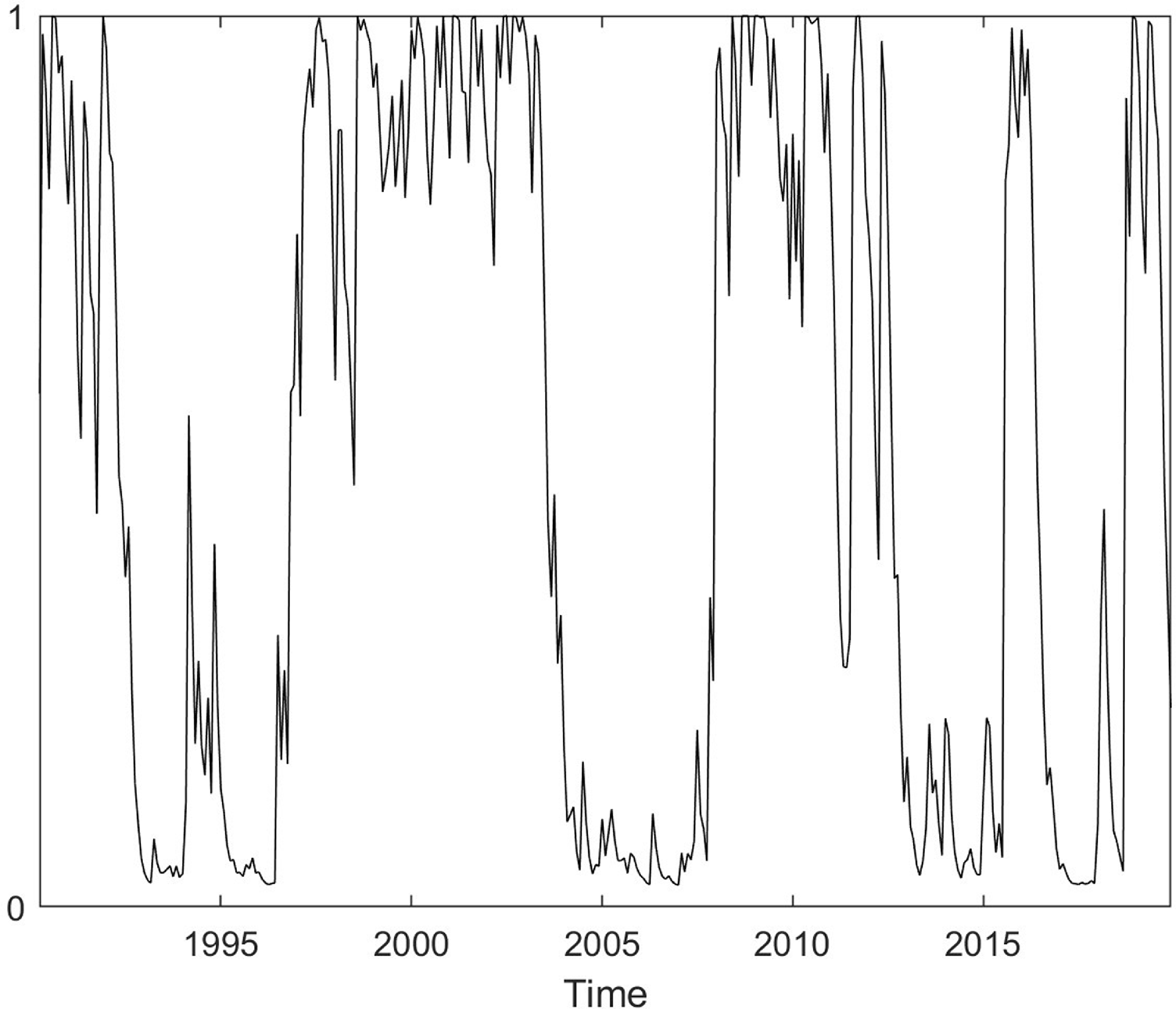
. These results indicate a high probability of remaining in the same state (0.9425 for fundamentalists and 0.9167 for trend followers), with a lower probability of transitioning between the two states (0.0575 from fundamentalists to chartists and 0.0833 in the opposite direction). These results indicate a high degree of persistence in agents’ behavioral regimes. Moreover, by applying filtering techniques to the latent state variable, we recover the time-varying regime probabilities, which serve as proxies for the relative weight assigned to each behavioral strategy over time. As illustrated in Figure 4, the trend-following regime exhibits dominance during periods of pronounced market stress – specifically, the dot-com bubble and the global financial crisis – whereas the fundamentalist regime gains prominence in the aftermath of these episodes, guiding market dynamics during the subsequent recovery phases.
$p_{cc}=0.9167$
. These results indicate a high probability of remaining in the same state (0.9425 for fundamentalists and 0.9167 for trend followers), with a lower probability of transitioning between the two states (0.0575 from fundamentalists to chartists and 0.0833 in the opposite direction). These results indicate a high degree of persistence in agents’ behavioral regimes. Moreover, by applying filtering techniques to the latent state variable, we recover the time-varying regime probabilities, which serve as proxies for the relative weight assigned to each behavioral strategy over time. As illustrated in Figure 4, the trend-following regime exhibits dominance during periods of pronounced market stress – specifically, the dot-com bubble and the global financial crisis – whereas the fundamentalist regime gains prominence in the aftermath of these episodes, guiding market dynamics during the subsequent recovery phases.
Filtered unobserved chartist state probability.

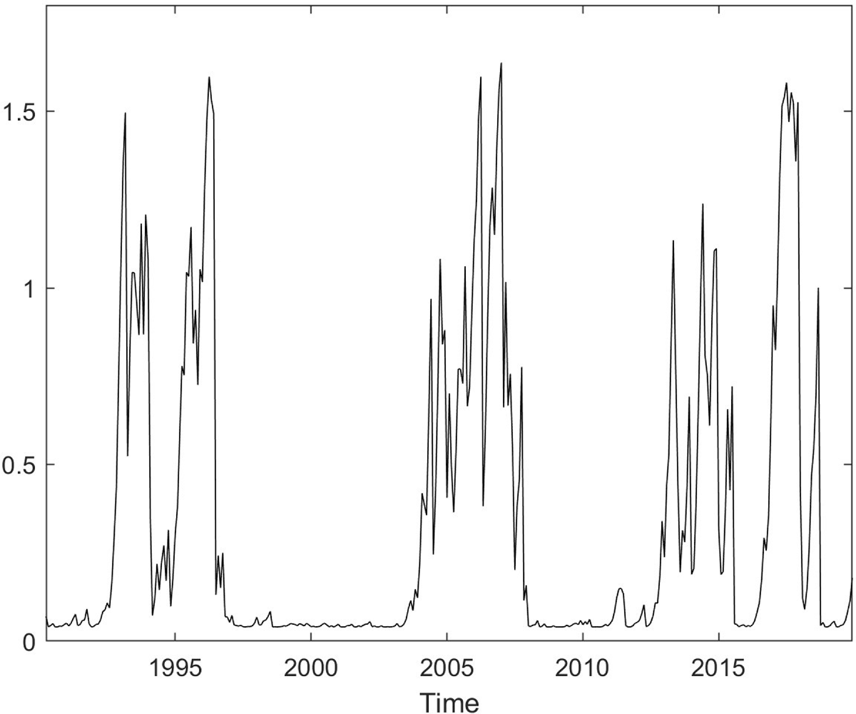
Reaction parameter of chartists in the nonlinear behavioral model.

As in the linear specification, the chartists’ reaction coefficient is derived from equation (8). Within the nonlinear framework, we use the Expectation-Maximization algorithm to jointly estimate the parameters
 $a_{11}$
and
$a_{11}$
and
 $a_{12}$
, while simultaneously filtering the time-varying probability of chartist dominance, denoted by
$a_{12}$
, while simultaneously filtering the time-varying probability of chartist dominance, denoted by
 $1-\delta$
. Given the structure of the system, the implied value of
$1-\delta$
. Given the structure of the system, the implied value of
 $\beta$
can be recovered as a function of these estimated components. Unlike the linear case, however,
$\beta$
can be recovered as a function of these estimated components. Unlike the linear case, however,
 $\beta$
evolves over time, reflecting regime-dependent dynamics, as shown in Figure 5.
$\beta$
evolves over time, reflecting regime-dependent dynamics, as shown in Figure 5.
The results reveal that high values of
 $\beta$
occur only during limited periods of time and quickly revert to lower levels. This contrasts with the linear specification, which imposes a constant reaction coefficient of
$\beta$
occur only during limited periods of time and quickly revert to lower levels. This contrasts with the linear specification, which imposes a constant reaction coefficient of
 $\beta = 1.74$
throughout the entire sample. These findings underscore the nonlinear model’s capacity to capture temporal changes that the linear model fails to address. In particular, the time-varying nature of
$\beta = 1.74$
throughout the entire sample. These findings underscore the nonlinear model’s capacity to capture temporal changes that the linear model fails to address. In particular, the time-varying nature of
 $\beta$
in the nonlinear model enhances its empirical realism by capturing shifts in agents’ responsiveness to past price trends.
$\beta$
in the nonlinear model enhances its empirical realism by capturing shifts in agents’ responsiveness to past price trends.
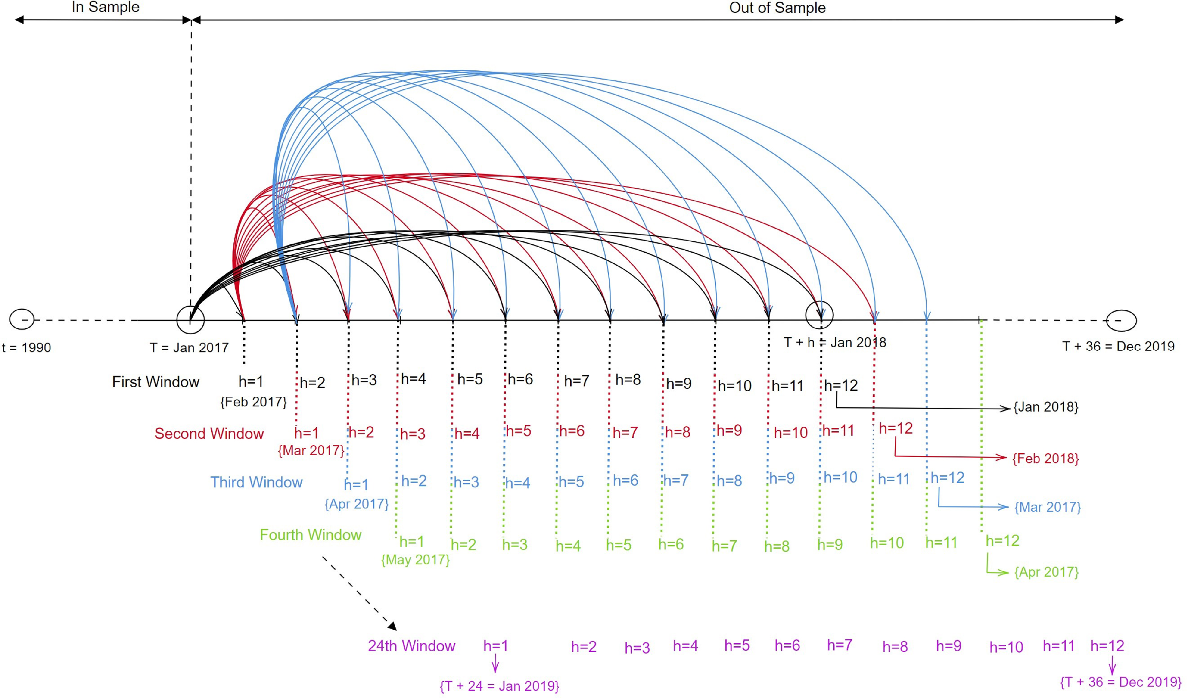
Rolling window forecasting procedure.

4. Out-of-sample comparison
After estimating the models, we proceed to compare the two, along with the benchmark random walk model, through an out-of-sample state-space analysis. We divide our data sample between Jan 1990 – Dec 2016 (in-sample period) and Jan 2017 – Dec 2019 (out-of-sample) so as to ensure many forecast observations to conduct inference. Concerning the linear forecasting procedure, the prediction error decomposition approach is repeated for all the out-of-sample periods in the forecasting exercise (Harvey, Reference Harvey2006). For the nonlinear version, we rely on the one-step-ahead point forecast for a MSDR model developed by Hamilton (Reference Hamilton1990).
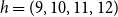
We implement a rolling window forecasting procedure across multiple horizons,
 $h = (1,2,3,\ldots 12)$
. This approach is adopted for three key reasons. First, it mitigates potential sensitivity to arbitrary sample splits by continuously updating the estimation sample. Second, it mimics the behavior of financial market participants who revise their expectations dynamically in response to incoming information. Third, it allows for a structured evaluation of model performance across different forecast horizons, distinguishing between short-term (
$h = (1,2,3,\ldots 12)$
. This approach is adopted for three key reasons. First, it mitigates potential sensitivity to arbitrary sample splits by continuously updating the estimation sample. Second, it mimics the behavior of financial market participants who revise their expectations dynamically in response to incoming information. Third, it allows for a structured evaluation of model performance across different forecast horizons, distinguishing between short-term (
 $h = (1,2,3,4)$
), medium-term (
$h = (1,2,3,4)$
), medium-term (
 $h = (5,6,7,8)$
), and long-term (
$h = (5,6,7,8)$
), and long-term (
 $h = (9,10,11,12)$
) intervals. The forecasting exercise is carried out using a fixed-size rolling estimation window of 325 monthly observations. At each iteration, the model is re-estimated using the most recent 325 data points, after which out-of-sample forecasts are generated for the subsequent
$h = (9,10,11,12)$
) intervals. The forecasting exercise is carried out using a fixed-size rolling estimation window of 325 monthly observations. At each iteration, the model is re-estimated using the most recent 325 data points, after which out-of-sample forecasts are generated for the subsequent
 $h$
-step horizon. The window is then advanced by one observation, and the process is repeated until the end of the forecasting period. See Figure 6 for a graphical explanation of the rolling window forecasting analysis.
$h$
-step horizon. The window is then advanced by one observation, and the process is repeated until the end of the forecasting period. See Figure 6 for a graphical explanation of the rolling window forecasting analysis.
Proceeding in this way, we estimate the model using the initial
 $325$
observations
$325$
observations
 $(p_1, p_2, \ldots , p_{325})$
, subsequently generating forecasts for the first
$(p_1, p_2, \ldots , p_{325})$
, subsequently generating forecasts for the first
 $h = 1,2,3,\ldots 12$
months ahead
$h = 1,2,3,\ldots 12$
months ahead
 $(p_{325+1}, p_{325+2}, \ldots , p_{325+12})$
. Likewise, we derive the subsequent
$(p_{325+1}, p_{325+2}, \ldots , p_{325+12})$
. Likewise, we derive the subsequent
 $h$
-month-ahead forecasts
$h$
-month-ahead forecasts
 $(p_{326+1}, p_{326+2}, \ldots , p_{326+12})$
by utilizing the data sequence
$(p_{326+1}, p_{326+2}, \ldots , p_{326+12})$
by utilizing the data sequence
 $p_2, p_3, \ldots , p_{326}$
. This iterative procedure continues until we generate the final
$p_2, p_3, \ldots , p_{326}$
. This iterative procedure continues until we generate the final
 $h$
-month-ahead forecasts
$h$
-month-ahead forecasts
 $(p_{348+1}, p_{348+2}, \ldots , p_{348+12})$
based on the observations
$(p_{348+1}, p_{348+2}, \ldots , p_{348+12})$
based on the observations
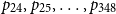 $p_{24}, p_{25}, \ldots , p_{348}$
. This recursion leads to a sequence
$p_{24}, p_{25}, \ldots , p_{348}$
. This recursion leads to a sequence
 $k_h=24$
for each forecasting horizon.
$k_h=24$
for each forecasting horizon.
Once the forecasting procedure has been implemented, the root mean square error (RMSE) and the mean absolute error (MAE) are calculated to compare the forecasting results for the different forecasting horizons. At the same time, we perform the Diebold-Mariano test to compare the predictive performance of different forecasts (Diebold and Mariano, Reference Diebold and Mariano1995). To perform it, we define the forecast errors with nonlinear Markov switching specification (NL) as:
 \begin{equation*}\varepsilon _{\left . {T + h} \right |T}^{NL} = {p_{T + h}} - p_{\left . {T + h} \right |T}^{NL},\end{equation*}
where
 $p_{T + h}$
and
$p_{T + h}$
and
 $p_{\left . {T + h} \right |T}$
are the actual and predicted values of asset prices respectively.
$p_{\left . {T + h} \right |T}$
are the actual and predicted values of asset prices respectively.
For the linear state-space specification (L):
 \begin{equation*}\varepsilon _{\left . {T + h} \right |T}^{L} = {p_{T + h}} - p_{\left . {T + h} \right |T}^{L},\end{equation*}
while for the random walk specification (RW):
 \begin{equation*}\varepsilon _{\left . {T + h} \right |T}^{RW} = {p_{T + h}} - p_{\left . {T + h} \right |T}^{RW},\end{equation*}
The loss associated with nonlinear, linear and random walk forecast is assumed to be a function
 $k$
of the forecast errors:
$k$
of the forecast errors:
 $k\big( {\varepsilon _{\left . {T + h} \right |T}^{NL}} \big)$
,
$k\big( {\varepsilon _{\left . {T + h} \right |T}^{NL}} \big)$
,
 $k\big( {\varepsilon _{{T + h} |T}^{L}} \big)$
and
$k\big( {\varepsilon _{{T + h} |T}^{L}} \big)$
and
 $k\big( {\varepsilon _{{T + h} |T}^{RW}} \big)$
respectively. We denote these functions with the squared-error loss and the absolute value. In this way, for the Markov switching dynamic regression model, we obtain:
$k\big( {\varepsilon _{{T + h} |T}^{RW}} \big)$
respectively. We denote these functions with the squared-error loss and the absolute value. In this way, for the Markov switching dynamic regression model, we obtain:
 \begin{equation*}k\left ( {\varepsilon _{\left . {T + h} \right |T}^{NL}} \right ) = {\left ( {\varepsilon _{\left . {T + h} \right |T}^{NL}} \right )^2}\quad {\rm and}\quad k\left ( {\varepsilon _{\left . {T + h} \right |T}^{NL}} \right ) = \left | {\varepsilon _{\left . {T + h} \right |T}^{NL}} \right |.\end{equation*}
For the linear state-space model:
 \begin{equation*}k\left ( {\varepsilon _{\left . {T + h} \right |T}^{L}} \right ) = {\left ( {\varepsilon _{\left . {T + h} \right |T}^{L}} \right )^2}\quad {\rm and}\quad k\left ( {\varepsilon _{\left . {T + h} \right |T}^{L}} \right ) = \left | {\varepsilon _{\left . {T + h} \right |T}^{L}} \right |.\end{equation*}
For the random walk model:
 \begin{equation*}k\left ( {\varepsilon _{\left . {T + h} \right |T}^{RW}} \right ) = {\left ( {\varepsilon _{\left . {T + h} \right |T}^{RW}} \right )^2}\quad {\rm and}\quad k\left ( {\varepsilon _{\left . {T + h} \right |T}^{RW}} \right ) = \left | {\varepsilon _{\left . {T + h} \right |T}^{RW}} \right |.\end{equation*}
Considering, for example, the NL and the L models, the loss differential between the two forecasts is:
 \begin{equation*}{d_{T + h}} = k\left ( {\varepsilon _{\left . {T + h} \right |T}^L} \right ) - k\left ( {\varepsilon _{\left . {T + h} \right |T}^{NL}} \right ).\end{equation*}
The two forecasts have equal accuracy if the loss differential has zero expectation for all
 $T + h$
. The null hypothesis states that the NL and L forecasts have the same predictive power:
$T + h$
. The null hypothesis states that the NL and L forecasts have the same predictive power:
 \begin{equation*}{H_0}\,:\,E\big( {{d_{T + h}}} \big) = 0\quad \forall ( {T + h} ).\end{equation*}
The alternative hypothesis states that the NL and L forecasts have different levels of performance:
 \begin{equation*}{H_1}\,:\,E\big( {{d_{T + h}}} \big) \ne 0.\end{equation*}
Under
 $H_0$
, the Diebold–Mariano test statistics is:
$H_0$
, the Diebold–Mariano test statistics is:
 \begin{equation*}\frac {{\bar{\!d} - u}}{{\sqrt {{\sigma ^2}/k_h} }} \to N\left ( {0,1} \right ).\end{equation*}
We repeat the test by comparing the three different specifications.
Let us start by comparing the linear state-space model and the random walk hypothesis.Footnote
14
Table 4 shows the results obtained. The columns represent the ratio of root mean squared error (RMSE) and the ratio of the mean absolute forecast error (MAE) of the linear model to that of the random walk model. A value greater than 1 indicates the superior performance of the random walk model. The parameter
 $h$
denotes the forecast horizon in months, and the Diebold-Mariano t-statistics are shown in parentheses.
$h$
denotes the forecast horizon in months, and the Diebold-Mariano t-statistics are shown in parentheses.
Out-of-sample forecast results (RW VS LSSM)
Notes:
 $^{*}$
,
$^{*}$
,
 $^{**}$
,
$^{**}$
,
 $^{***}$
denote statistical significance at the 10, 5, and 1% levels respectively.
$^{***}$
denote statistical significance at the 10, 5, and 1% levels respectively.
Let us first examine the RMSE results. From Table 4, we can observe that the behavioral linear model has an inferior performance compared to the random walk forecasts. Overall, the exogenous linear model outperforms the endogenous behavioral linear specification. More in the details, from 1 monthly horizon up to 12 monthly horizon, the RMSE ratio is above the unity and these results are statistically significant at the one percent level according to the Diebold-Mariano test. Passing to the MAE analysis, the ratio is consistently greater than one at the one percent statistical level, indicating significant differences in the predictive accuracy.
To summarize, the random walk model outperforms the linear state-space model in the short-term (
 $h =1, 2, 3, 4$
months), medium-term (
$h =1, 2, 3, 4$
months), medium-term (
 $h =5, 6, 7, 8$
months), and long-term (
$h =5, 6, 7, 8$
months), and long-term (
 $h =9, 10, 11, 12$
months) forecasts out-of-sample analysis. Nevertheless, we observe an interesting pattern from Table 4. As the forecasting horizon extends from short-term (
$h =9, 10, 11, 12$
months) forecasts out-of-sample analysis. Nevertheless, we observe an interesting pattern from Table 4. As the forecasting horizon extends from short-term (
 $h =1$
month) to longer-term (
$h =1$
month) to longer-term (
 $h =12$
months), the ratio exhibits a consistent downward trend, gradually approaching a value of 1. This pattern suggests the presence of a convergence phenomenon, where the predictive performance of the linear behavioral model gradually improves relative to the random walk as the forecast horizon extends. Over longer horizons, the random walk’s advantage fades, eventually disappearing. This result is consistent with the idea of linear convergence toward a long-run equilibrium, as implied by the dynamics of the state-space framework.Footnote
15
$h =12$
months), the ratio exhibits a consistent downward trend, gradually approaching a value of 1. This pattern suggests the presence of a convergence phenomenon, where the predictive performance of the linear behavioral model gradually improves relative to the random walk as the forecast horizon extends. Over longer horizons, the random walk’s advantage fades, eventually disappearing. This result is consistent with the idea of linear convergence toward a long-run equilibrium, as implied by the dynamics of the state-space framework.Footnote
15
Table 5 presents the outcomes of the out-of-sample forecast comparison between the nonlinear Markov switching dynamic regression model and the linear state-space model. As before, we examine the predictive performance of these two models across different forecast horizons, from
 $h=1$
to
$h=1$
to
 $h=12$
months, and considering the ratio of RMSE and MAE of the nonlinear Markov model to the linear state-space model. The results are consistent with the previous findings and reveal a robust pattern: the Markov-switching specification systematically outperforms the linear behavioral model across all forecast horizons. This superior performance underscores the nonlinear model’s enhanced capacity to capture time-varying dynamics and structural shifts in agents’ behavior, which are not adequately addressed by the linear framework.Footnote
16
Both for RMSE and MAE metrics, this trend extends across short (
$h=12$
months, and considering the ratio of RMSE and MAE of the nonlinear Markov model to the linear state-space model. The results are consistent with the previous findings and reveal a robust pattern: the Markov-switching specification systematically outperforms the linear behavioral model across all forecast horizons. This superior performance underscores the nonlinear model’s enhanced capacity to capture time-varying dynamics and structural shifts in agents’ behavior, which are not adequately addressed by the linear framework.Footnote
16
Both for RMSE and MAE metrics, this trend extends across short (
 $h =1, 2, 3, 4$
months), medium (
$h =1, 2, 3, 4$
months), medium (
 $h =5, 6, 7, 8$
months) and long forecast horizons (
$h =5, 6, 7, 8$
months) and long forecast horizons (
 $h =9, 10, 11, 12$
months), implying that the predictive power of the nonlinear model remains robust across different prediction periods at one percent statistical value for the Diebold Mariano test.
$h =9, 10, 11, 12$
months), implying that the predictive power of the nonlinear model remains robust across different prediction periods at one percent statistical value for the Diebold Mariano test.
Out-of-sample forecast results (NLMS VS LSSM)

Notes:
 $^{*}$
,
$^{*}$
,
 $^{**}$
,
$^{**}$
,
 $^{***}$
denote statistical significance at the 10%, 5%, and 1% levels respectively.
$^{***}$
denote statistical significance at the 10%, 5%, and 1% levels respectively.
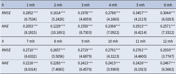
Out-of-sample forecast results (NLMS VS RW)
Notes:
 $^{*}$
,
$^{*}$
,
 $^{**}$
,
$^{**}$
,
 $^{***}$
denote statistical significance at the 10, 5, and 1% levels respectively.
$^{***}$
denote statistical significance at the 10, 5, and 1% levels respectively.
Overall, the obtained results confirm the importance of considering switching processes in the beliefs of the agents so as to generate nonlinear local endogenous fluctuations phenomena.
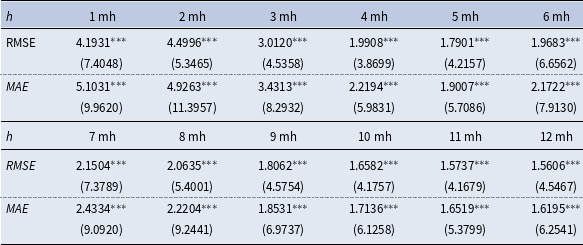
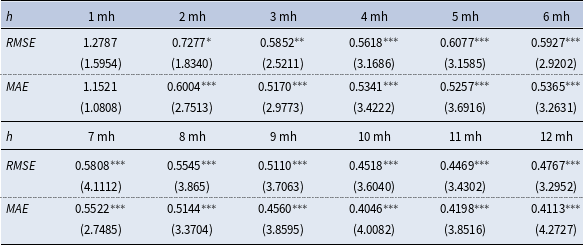
Finally, we compare the out-of-sample forecasting power of the nonlinear Markov switching dynamic regression model with that of the random walk model. The results in Table 6 show that the random walk outperforms the behavioral nonlinear model only for the first short period. Furthermore, for
 $h=1$
, the RMSE ratio is equal to 1.2787 but not statistically significant for the Diebold Mariano test. Moreover, from the second period onward, the behavioral nonlinear model outperforms significantly better than the random walk model. For
$h=1$
, the RMSE ratio is equal to 1.2787 but not statistically significant for the Diebold Mariano test. Moreover, from the second period onward, the behavioral nonlinear model outperforms significantly better than the random walk model. For
 $h=2$
, the RMSE ratio equals 0.7277 and is significant at ten percent level. For
$h=2$
, the RMSE ratio equals 0.7277 and is significant at ten percent level. For
 $h=3$
, the ratio is 0.5852 and statistically significant at five percent level. From
$h=3$
, the ratio is 0.5852 and statistically significant at five percent level. From
 $h=4, \ldots 12$
, the ratio tends to decrease, highlighting an increasingly better performance of the nonlinear behavioral model compared to the linear random walk model at one percent level. With respect to MAE, we obtain similar results; for the forecasting horizon
$h=4, \ldots 12$
, the ratio tends to decrease, highlighting an increasingly better performance of the nonlinear behavioral model compared to the linear random walk model at one percent level. With respect to MAE, we obtain similar results; for the forecasting horizon
 $h = 1$
month, the ratio is greater than one, but not statistically significant. The opposite for
$h = 1$
month, the ratio is greater than one, but not statistically significant. The opposite for
 $h = 2, 3, 4, \ldots , 12$
, where the ratio is smaller than one and statistically significant at one percent level.
$h = 2, 3, 4, \ldots , 12$
, where the ratio is smaller than one and statistically significant at one percent level.
To summarize the key finding of our analysis, the proposed NLMS model can beat the behavioral linear model and the exogenous linear model at very different forecasting horizons, both in the short (from
 $h=2$
), medium and long run.
$h=2$
), medium and long run.
5. Conclusions
This paper has analyzed the impact of unobserved speculative strategies of agents on the determination of asset price dynamics. To this end, we (i) transformed the heterogeneous agent setting into a linear state-space form and, based on this, retrieved the mathematical condition for complex eigenvalues, (ii) moved to a nonlinear Markov setting to highlight possible local instability phenomena and, finally, (iii) compared the linear and nonlinear out-of-sample forecasting power with the benchmark random walk model.
Among our main findings, we have highlighted the presence of speculative behavior that generates endogenous fluctuations in the price formation process. Moreover, the out-of-sample forecasts of the nonlinear heterogeneous agent model significantly outperform those of both the linear heterogeneous agent model and the benchmark random walk model at the short, medium and long horizons. These results contribute to the growing body of literature that argues that financial instability cannot be viewed as a simple exogenous phenomenon, but as an endogenous process generated by the time-varying speculative strategies of heterogeneous agents.
The methodology we use could be extended in different directions. One interesting venue of future research consists in the introduction of additional heuristics, such as noise trading or a contrarian strategy. Moreover, the analysis could be extended to other financial markets, such as the exchange rate market. Finally, it would be worth moving from a uni-variate to a multivariate model in which the real side of the economy interacts with the stock market. In this way, we could identify channels of transmission of speculative phenomena in the financial markets to the real economy and vice versa. While these extensions are undoubtedly promising, they would require alternative state-space formulations with distinct cyclical properties. We therefore leave these developments to future research.
Acknowledgments
We are grateful to the editor and the two anonymous reviewers for their insightful comments and constructive criticism, which significantly improved the paper. We thank Thomas Lux for invaluable discussions and comments that helped shape the idea behind the paper and refine the exposition. We also thank Yuri Basile for helping us on data management. The usual disclaimer applies. Filippo Gusella is grateful for financial support from the Università di Firenze, the Complexity Lab in Economics (CLE), Università Cattolica del Sacro Cuore, and the Fondazione Cassa di Risparmio di Pistoia e Pescia.
Supplementary material
The supplementary material for this article can be found at http://dx.doi.org/10.1017/S1365100525100345.


 Open access