


1. Introduction
Subdwarf B stars (hereafter sdB) are understood as low-mass stars in late stages of evolution, stripped of most of their hydrogen-rich envelope and stably burning helium in their cores while located at the hot end of the horizontal branch of the Hertzsprung-Russell diagram (the so-called extreme horizontal branch). They were first defined by Sargent & Searle (Reference Sargent and Searle1968) and an overview of their properties can be found in the recent review by Heber (Reference Heber2016). Although formation scenarios from single stellar evolution have been proposed for sdBs (such as the hot flasher case, see D’Cruz et al. Reference D’Cruz, Dorman, Rood and O’Connell1996), binary evolution provides the most widely accepted formation channels. This is supported by the large fraction of observed sdBs that are members of a binary system (see e.g. Maxted et al. Reference Maxted, Heber, Marsh and North2001; Stark & Wade Reference Stark and Wade2003; Pelisoli et al. Reference Pelisoli, Vos, Geier, Schaffenroth and Baran2020, and references therein), and by how binary interactions can explain the method through which a star is capable of losing a large fraction of its outer hydrogen-rich layers. Additionally, the existence of single sdBs does not contradict the binary-related formation channels, since single sdBs can also be explained through binary evolution, due to the merger of two helium white dwarfs (He WDs, see i.e. Tutukov et al. Reference Tutukov, Fedorova, Ergma and Yungelson1985). For more discussion about the formation channels, see (Han et al. Reference Han, Podsiadlowski, Maxted, Marsh and Ivanova2002, Reference Han, Podsiadlowski, Maxted and Marsh2003, abbreviated as H02 and H03 throughout the paper).
Around one-third of sdBs in the observational sample have short orbital periods (Pelisoli et al. Reference Pelisoli, Vos, Geier, Schaffenroth and Baran2020) and, within this group, there are many sdB + white dwarf (WD) systems which are thought to lead to energetic transient phenomena such as double detonation type Ia supernovae (see e.g. Nomoto Reference Nomoto1982; Livne Reference Livne1990; Woosley & Weaver Reference Woosley and Weaver1994; Neunteufel, Yoon, & Langer Reference Neunteufel, Yoon and Langer2016 for details, or Kupfer et al. Reference Kupfer2022 for a recently proposed double-detonation progenitor) or AM CVn systems (e.g. Savonije, de Kool, & van den Heuvel Reference Savonije, de Kool and van den Heuvel1986; Iben & Tutukov Reference Iben and Tutukov1987; Bauer & Kupfer Reference Bauer and Kupfer2021), when helium-rich material is transferred from the sdB onto the WD. Another important consequence of these small orbits is that such short periods might produce gravitational waves detectable by the upcoming Laser Interferometer Space Antenna (LISA, Amaro-Seoane et al. Reference Amaro-Seoane2023), an example of which is CD–30 $^\circ$
11223 (Geier et al. Reference Geier2013; Kupfer et al. Reference Kupfer2018).
$^\circ$
11223 (Geier et al. Reference Geier2013; Kupfer et al. Reference Kupfer2018).
The importance of sdBs in the context of binary evolution is therefore clear, but it should be noted that their relevance extends further. For example, they have been used in studies of the observed UV upturn of elliptical galaxies (e.g. Brown Reference Brown2004) and old stellar populations, as well as in the context of asteroseismological studies owing to the different modes in which they have been observed to pulsate (e.g. Reed et al. Reference Reed2021). In a similar vein of variable star research, sdBs have also been proposed as potential progenitors of the recently discovered blue large-amplitude pulsator (BLAP) class of pulsating stars (Pietrukowicz et al. Reference Pietrukowicz2017), which would correspond to an sdB’s helium shell burning stage after helium has been depleted in the core and the star moves towards the subdwarf O star location in the Hertzsprung-Russell diagram (for details, see Xiong et al. Reference Xiong2022).
All of these elements imply that there is a need for a better understanding of the formation and evolution of sdB systems. For this purpose, binary population synthesis (BPS) has been historically used as a statistical tool to study sdB formation channels (e.g. Han et al. Reference Han, Podsiadlowski, Maxted and Marsh2003; Nelemans Reference Nelemans2010; Clausen et al. Reference Clausen, Wade, Kopparapu and O’Shaughnessy2012; Chen et al. Reference Chen, Han, Deca and Podsiadlowski2013), finding general agreement with observed properties such as the orbital period and mass distribution of the current day population. Despite this, rapid BPS by design requires a large number of parametrisable quantities, making it difficult to set a unique set of input physics that can accurately reproduce the observational results (but see Toonen et al. Reference Toonen, Claeys, Mennekens and Ruiter2014, for a BPS parameter study applied to double WD systems). Instead, it is possible to get an idea of what parameters play a greater role on recovering observed properties of a given population, and also what elements are present in the final populations in multiple different configurations, hinting at a higher likelihood of their occurrence in real populations.
In this paper, we use the rapid BPS code Compact Object Mergers: Population Astrophysics and Statistics (compas, Team COMPAS: Riley et al. Reference Riley2022) and results from Modules for Experiments in Stellar Astrophysics (mesa, Paxton et al. Reference Paxton2011, Reference Paxton2013, Reference Paxton2015, Reference Paxton2018, Reference Paxton2019) to explore the impact of varying the initial parameters when studying sdBs through binary population synthesis, as well as the effects that these parameters have on the proposed sdB formation channels from binary star evolution.
Section 2 contains the description of the method and software used in our work, particularly details about our BPS approach and parameter variation in Section 2.1, as well as relevant methods related to detailed stellar models in Section 2.2. The results are then shown in Section 3, which is organised as follows: the effects of varying parameters in Section 3.1, the sdB-formation channels in Section 3.2, and a comparison to similar studies available in the literature in Section 3.3. We provide our summary and conclusions in Section 4.
2. Method, software and input physics
2.1. Binary population synthesis
To create our binary populations we use compas v02.50.00 (Team COMPAS: Riley et al. Reference Riley2022), an open source rapid BPS software capable of generating populations of stellar binary systems under a set of parameterised prescriptions that describe the evolution and interaction of their components. Similar to other BPS codes such as bse (Hurley, Tout, & Pols Reference Hurley, Tout and Pols2002), startrack (Belczynski et al. Reference Belczynski2008), binary_c (Izzard et al. Reference Izzard, Tout, Karakas and Pols2004), seba (Toonen, Nelemans, & Portegies Zwart Reference Toonen, Nelemans and Portegies Zwart2012) or cosmic (Breivik et al. Reference Breivik2020), compas is capable of quickly evolving millions of stellar binary systems in a few CPU hours thanks to its efficient code and simplified prescriptions, allowing statistical studies and tests of the selected physical configuration at the expense of detailed physics like what is done through 1D stellar evolution models produced by software such as mesa, or hydro-dynamical codes (e.g. Price et al. Reference Price2018). We also highlight that, so far, compas has been mostly used to study compact objects: remnants resulting in neutron stars or black holes (e.g. Broekgaarden et al. Reference Broekgaarden2022; Stevenson & Clarke Reference Stevenson and Clarke2022; Wagg et al. Reference Wagg2022). Here we study sdBs (which have masses below $1~\mathrm{M}_\odot$
, typically around
$1~\mathrm{M}_\odot$
, typically around $0.5~\mathrm{M}_\odot$
), effectively using compas to study low-mass non-compact remnants for the first time. Our results will thus set the stage for future compas research involving stars and their products at the low- and intermediate-mass end of the initial mass function.
$0.5~\mathrm{M}_\odot$
), effectively using compas to study low-mass non-compact remnants for the first time. Our results will thus set the stage for future compas research involving stars and their products at the low- and intermediate-mass end of the initial mass function.
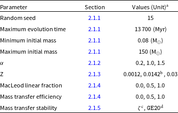
To analyse the different sdB formation pathways, similar to what has been done in previous studies (e.g. H03; Clausen et al. Reference Clausen, Wade, Kopparapu and O’Shaughnessy2012), we perform a parameter study and we use a total of 162 different combinations of parameters (see Appendix A for details of each). Most configurable parameters in compas have not been modified, except for those directly specified in Table 1. All of the parameters included in this table are discussed in the following sections.
Set of parameters used to construct our different compas population synthesis realisations. A single value (third column) implies that the property was changed from its default value (defined in Riley et al. Reference Riley2022), but kept fixed on all our runs.
 $^{\textrm{a}}$
Only when applicable.
$^{\textrm{a}}$
Only when applicable. $^{\textrm{b}}$
Default (solar) value in compas, following Asplund et al. (Reference Asplund, Grevesse, Sauval and Scott2009).
$^{\textrm{b}}$
Default (solar) value in compas, following Asplund et al. (Reference Asplund, Grevesse, Sauval and Scott2009). $^{\textrm{c}}$
e.g. Soberman et al. (Reference Soberman, Phinney and van den Heuvel1997) or Woods et al. (Reference Woods, Ivanova, van der Sluys and Chaichenets2012) for a more recent analysis.
$^{\textrm{c}}$
e.g. Soberman et al. (Reference Soberman, Phinney and van den Heuvel1997) or Woods et al. (Reference Woods, Ivanova, van der Sluys and Chaichenets2012) for a more recent analysis. $^{\textrm{d}}$
Critical mass ratios as in Ge et al. (Reference Ge, Webbink, Chen and Han2020), under the adiabatic assumption.
$^{\textrm{d}}$
Critical mass ratios as in Ge et al. (Reference Ge, Webbink, Chen and Han2020), under the adiabatic assumption.
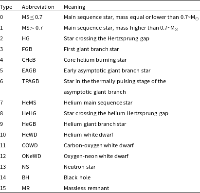
Summary of the Hurley, Pols, & Tout (Reference Hurley, Pols and Tout2000) stellar types. For simplicity, we use the abbreviations through the text and figures.
Kiel diagram for a sample of known sdBs, where blue circles correspond to Culpan et al. (Reference Culpan2022) and orange triangles to Lei et al. (Reference Lei2023). Their reported uncertainties are shown as light grey lines. The box delimited by black solid lines corresponds to the selection criteria chosen as our definition of sdB candidates from the compas sample and is explicitly defined in Section 2.1.
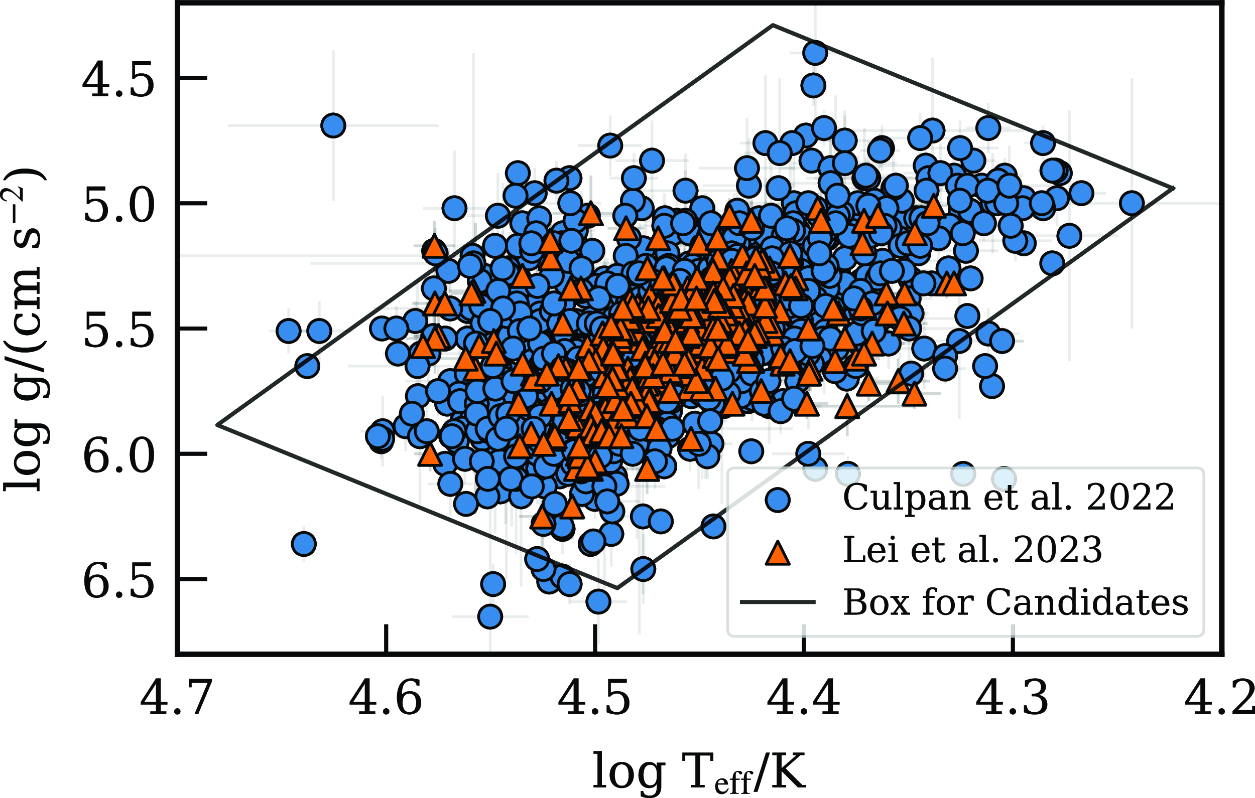
Our sample of sdB candidates is built by collecting stars flagged as type 7 at any given time during their evolution, that is, they have gone through the naked helium main sequence (HeMS) as per the compas notation for stellar types (see Table 2 for the definition of each stellar type, inherited from Hurley et al. Reference Hurley, Pols and Tout2000). On top of that, we also require our sample to match or be approximately equal to the observational results (as seen in Fig. 1), effectively imposing a restriction on the size and temperature of each candidate. This criterion is enforced by selecting HeMS stars that cross the area in the Kiel diagram delimited by the following equations:
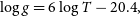 \begin{align} \log{g} = 6\log{T} - 20.4,\end{align}
 \begin{align} \log{g} = 6\log{T} - 22.4, \end{align}
 \begin{align} \log{g} = -3.4\log{T} + 21.8,\end{align}
 \begin{align} \log{g} = -3.4\log{T} + 19.3,\end{align}
where T is the effective temperature (in Kelvins) and g surface gravity (in cm s $^{-2}$
) of a given star. This has been defined by visual inspection of the Culpan et al. (Reference Culpan2022) observational sdB sample, and further checked against the Lei et al. (Reference Lei2023) sdB catalog as seen in Fig. 1. Note that this method allows for the existence of stars that are not necessarily born, or stay during their entire lifetimes, as our observational definition of sdB candidates.
$^{-2}$
) of a given star. This has been defined by visual inspection of the Culpan et al. (Reference Culpan2022) observational sdB sample, and further checked against the Lei et al. (Reference Lei2023) sdB catalog as seen in Fig. 1. Note that this method allows for the existence of stars that are not necessarily born, or stay during their entire lifetimes, as our observational definition of sdB candidates.
We also select some candidates from stars flagged as type 10 (helium white dwarfs, HeWD), only when we want to analyse the impact of allowing helium ignition in HeWDs with masses within 5% or 3% of the expected core mass the progenitor would have attained at the tip of the red giant branch (RGB, used as a synonym of FGB defined in Table 2), owing to the results of D’Cruz et al. (Reference D’Cruz, Dorman, Rood and O’Connell1996), H02 and Clausen et al. (Reference Clausen, Wade, Kopparapu and O’Shaughnessy2012). These stars are then evolved as HeMS stars during post processing, and follow the same selection criteria based on observational constraints as HeMS stars do.
A final important consideration is that within our candidates we do not include systems that merge right after a mass transfer event, nor do we track the evolution of the companions. This last element is a consequence of our post-processing approach to the evolution of the sdB candidates, as will be explained in Section 2.2.1.
2.1.1. Initial parameters
Both initial masses and orbital configuration (orbital periods and eccentricities) for all our systems are sampled following the correlated distributions presented in Moe & Di Stefano (Reference Moe and Di Stefano2017). This process is implemented in the sampleMoeDiStefano.py script distributed as part of the pre-processing tools in compas. The only parameter that we have customised in this script is the mass range, which we have set to 0.08–150 $\,\mathrm{M}_\odot$
for the initial mass of the primary star to allow all possible progenitors: non-zero accretion efficiency allows low-mass stars to evolve faster (eventually becoming sdB candidates) as a consequence of an accretion episode, while setting a rather high upper mass limit allows for a higher chance of sampling massive primaries. About 1 000 000 stellar systems are produced, though this also includes single stars that are not evolved by compas when using its binary population synthesis mode. After removing these, our binary population consists of
$\,\mathrm{M}_\odot$
for the initial mass of the primary star to allow all possible progenitors: non-zero accretion efficiency allows low-mass stars to evolve faster (eventually becoming sdB candidates) as a consequence of an accretion episode, while setting a rather high upper mass limit allows for a higher chance of sampling massive primaries. About 1 000 000 stellar systems are produced, though this also includes single stars that are not evolved by compas when using its binary population synthesis mode. After removing these, our binary population consists of $\sim$
284 000 systems, which will be evolved using the 162 different configurations previously mentioned.
$\sim$
284 000 systems, which will be evolved using the 162 different configurations previously mentioned.
2.1.2. Common envelope
The compas code adopts the energy formalism for common envelope (CE, Webbink Reference Webbink1984; de Kool Reference de Kool1990), which requires setting the $\alpha$
and
$\alpha$
and $\lambda$
parameters as indicated by the equations
$\lambda$
parameters as indicated by the equations
 \begin{align} E_{\mathrm{bind}} = \alpha \, \Delta E_{\mathrm{orb}},\end{align}
 \begin{align} E_{\mathrm{bind}} = - \frac{GMM_{\mathrm{env}}}{\lambda R},\end{align}
where $E_{\mathrm{bind}}$
is the gravitational binding energy of the envelope,
$E_{\mathrm{bind}}$
is the gravitational binding energy of the envelope, $\alpha$
is an efficiency parameter that specifies the fraction of orbital energy used to remove the CE,
$\alpha$
is an efficiency parameter that specifies the fraction of orbital energy used to remove the CE, $\Delta E_{\mathrm{orb}}$
corresponds to the change in orbital energy due to the CE phase, and
$\Delta E_{\mathrm{orb}}$
corresponds to the change in orbital energy due to the CE phase, and $\lambda$
is a structure parameter that represents the relationship of the binding energy of the stellar envelope and the location of its inner boundary, as well as the sources of energy considered for its removal (for a recent review on numerical techniques relevant for CE evolution, see Röpke & De Marco Reference Röpke and De Marco2023).
$\lambda$
is a structure parameter that represents the relationship of the binding energy of the stellar envelope and the location of its inner boundary, as well as the sources of energy considered for its removal (for a recent review on numerical techniques relevant for CE evolution, see Röpke & De Marco Reference Röpke and De Marco2023).
For $\lambda$
we use the default configuration in compas, i.e. the Xu & Li (Reference Xu and Li2010a, b
) prescription implemented through fitting formulae to results of detailed stellar models, considering the full contribution of internal energy (Team COMPAS: Riley et al. Reference Riley2022). In the case of
$\lambda$
we use the default configuration in compas, i.e. the Xu & Li (Reference Xu and Li2010a, b
) prescription implemented through fitting formulae to results of detailed stellar models, considering the full contribution of internal energy (Team COMPAS: Riley et al. Reference Riley2022). In the case of $\alpha$
we explore the set of values presented in Table 1, as the current constraints on envelope removal efficiency are poor (De Marco et al. Reference De Marco2011), and therefore it is useful to explore different possible values. Zorotovic et al. (Reference Zorotovic, Schreiber, Gänsicke and Nebot Gómez-Morán2010) point towards
$\alpha$
we explore the set of values presented in Table 1, as the current constraints on envelope removal efficiency are poor (De Marco et al. Reference De Marco2011), and therefore it is useful to explore different possible values. Zorotovic et al. (Reference Zorotovic, Schreiber, Gänsicke and Nebot Gómez-Morán2010) point towards $\alpha_{\mathrm{CE}} \sim 0.2$
, while we also consider full efficiency (
$\alpha_{\mathrm{CE}} \sim 0.2$
, while we also consider full efficiency ( $\alpha = 1$
) and the possible contribution of additional energy sources with
$\alpha = 1$
) and the possible contribution of additional energy sources with $\alpha = 1.5$
(see e.g. Ivanova, Justham, & Ricker Reference Ivanova, Justham and Ricker2020).
$\alpha = 1.5$
(see e.g. Ivanova, Justham, & Ricker Reference Ivanova, Justham and Ricker2020).
2.1.3. Metallicity
The importance of metallicity in the formation of sdBs can be understood from a few different angles. First, changes on metallicity modify the initial mass – core mass relation close to the tip of the RGB (see e.g. Cassisi, Salaris, & Pietrinferni Reference Cassisi, Salaris and Pietrinferni2016), affecting the observed sdB mass distribution by changing the core mass value near the tip of the RGB. This core mass is the one that directly sets the mass of a given sdB, as it represents most of what remains of the progenitor star after removing its outer layers. It must be noted that other parameters such as the overshooting prescription might play an important role in setting the initial mass – core mass relation as well (e.g. Arancibia-Rojas et al. Reference Arancibia-Rojas2024, and references therein). Next, the mass limit for the ignition of helium in a flash (MHeF) is also affected by changes on metallicity. Sweigart & Gross (Reference Sweigart and Gross1978) show that the critical mass threshold for a helium flash to occur is lowered with decreasing metallicity. This affects the initial mass and proprieties of the newly born sdB, particularly in the context of rapid BPS codes that have inherited the Hurley et al. (Reference Hurley, Pols and Tout2000) methods where the evolution of a HeMS star (used as an sdB proxy) depends solely on its initial mass. Note that while the critical mass is reduced, the core mass near the tip of the RGB for a given zero age main sequence (ZAMS) value is increased. Finally, the size of the progenitor (the donor) impacts the likelihood of Roche Lobe Overflow (RLOF) and therefore mass transfer, as well as its stability (e.g. Chen et al. Reference Chen, Han, Deca and Podsiadlowski2013; Vos, Bobrick, & Vučković Reference Vos, Bobrick and Vučković2020). The role played by metallicity is relevant, though the growth of the stellar radius during the RGB phase is still a topic of discussion (e.g. Renzini Reference Renzini2023).
To explore its effects on the final sdB yields, our BPS realisations include three different metallicities, namely sub-solar, solar, and super-solar. The specific values were chosen considering both compas limits and the study of long period sdBs in Vos et al. (2020), which considers the different structural components of the Galaxy. Their metallicities are shown as iron abundance relative to hydrogen (i.e. [Fe/H]) and are closer to a continuous distribution, while we use a discrete set of 3 values (see Table 1) and relate [Fe/H] to nominal Z input values for compas. This was done by using a simplified approach (e.g. Equation 9 in Bertelli et al. Reference Bertelli, Bressan, Chiosi, Fagotto and Nasi1994, assuming that $X\approx X_\odot$
):
$X\approx X_\odot$
):
 \begin{equation} \left[\mathrm{Fe/H}\right] \approx \log{Z/Z_\odot},\end{equation}
which approximately transforms the range $-1.08 \leq \left[\mathrm{Fe/H}\right] \leq 0.4 $
covered in table 1 of Vos et al. (2020) to
$-1.08 \leq \left[\mathrm{Fe/H}\right] \leq 0.4 $
covered in table 1 of Vos et al. (2020) to $0.0012 \leq Z \leq 0.036$
, by assuming
$0.0012 \leq Z \leq 0.036$
, by assuming $Z_\odot = 0.0142$
(Asplund et al. Reference Asplund, Grevesse, Sauval and Scott2009) as implemented in compas (Team COMPAS: Riley et al. Reference Riley2022). The final values that we use consider these results (limited by the maximum/minimum allowed metallicity value in compas), as well as solar metallicity. We have ignored the metallicity value related to the halo component, as it does not seem to play a critical role for the Galactic sdB population (consider its mass fraction in table 1 of Vos et al. Reference Vos, Bobrick and Vučković2020).
$Z_\odot = 0.0142$
(Asplund et al. Reference Asplund, Grevesse, Sauval and Scott2009) as implemented in compas (Team COMPAS: Riley et al. Reference Riley2022). The final values that we use consider these results (limited by the maximum/minimum allowed metallicity value in compas), as well as solar metallicity. We have ignored the metallicity value related to the halo component, as it does not seem to play a critical role for the Galactic sdB population (consider its mass fraction in table 1 of Vos et al. Reference Vos, Bobrick and Vučković2020).
2.1.4. Orbital angular momentum loss and mass transfer efficiency
We assume that the specific angular momentum carried away by any amount of mass being lost from the system is a fraction of the total specific angular momentum, represented by
 \begin{align} h_{\mathrm{lost}} = \gamma \frac{J}{M_{a} + M_{d}}, \end{align}
 \begin{align} J = M_{a}M_{d}\sqrt{\frac{Ga\left(1-e^2\right)}{\left(M_{a} + M_{d}\right)}},\end{align}
with $h_{\mathrm{lost}}$
the specific angular momentum being lost, J the total orbital angular momentum of the system, G the gravitational constant, a the semi-major axis, e the eccentricity and
$h_{\mathrm{lost}}$
the specific angular momentum being lost, J the total orbital angular momentum of the system, G the gravitational constant, a the semi-major axis, e the eccentricity and $M_{x}$
is the mass of the donor (d) or accretor (a). Note that e can be taken as 0 here, since compas circularises orbits right before mass transfer events (a common practice in rapid BPS codes).
$M_{x}$
is the mass of the donor (d) or accretor (a). Note that e can be taken as 0 here, since compas circularises orbits right before mass transfer events (a common practice in rapid BPS codes). $\gamma$
represents a coefficient that specifies the fraction of specific angular momentum being lost, and it depends on the position at which mass is being lost from the system. This can be expressed as
$\gamma$
represents a coefficient that specifies the fraction of specific angular momentum being lost, and it depends on the position at which mass is being lost from the system. This can be expressed as
 \begin{align} h_{\mathrm{lost}} = a_{\mathrm{lost}}^2\omega, \end{align}
 \begin{align} \omega \equiv \frac{2\pi}{P} = \sqrt{\frac{G\left(M_{a} + M_{d}\right)}{a^3}},\end{align}
where $\omega$
is the orbital frequency and P its orbital period. All other elements are the same as in Equation (9). Then, by combining Equations (8), (9) and (10) we can find an expression for
$\omega$
is the orbital frequency and P its orbital period. All other elements are the same as in Equation (9). Then, by combining Equations (8), (9) and (10) we can find an expression for $\gamma$
. Explicitly,
$\gamma$
. Explicitly,
 \begin{equation} \gamma = \left(\frac{a_\textrm{lost}}{a}\right)^2 \frac{\left(M_{a} + M_{d}\right)^2}{M_{a}M_{ d}\sqrt{1-e^2}},\end{equation}
which shows the dependence on where mass is being lost from (by setting the appropriate $a_{\mathrm{lost}}$
value).
$a_{\mathrm{lost}}$
value).
This framework has been implemented within the MACLEOD_LINEAR prescription in compas (Willcox et al. Reference Willcox, MacLeod, Mandel and Hirai2023), where instead of setting $a_\textrm{lost}$
we can set the linear variable –mass-transfer-jloss-macleod-linear-fraction
Footnote
a
(MLF; MacLeod Linear Fraction) with values between 0 and 1, corresponding to
$a_\textrm{lost}$
we can set the linear variable –mass-transfer-jloss-macleod-linear-fraction
Footnote
a
(MLF; MacLeod Linear Fraction) with values between 0 and 1, corresponding to $a_{\mathrm{obj}} \in \left[a_{\mathrm{acc}}, L_2\right]$
(the position of the accretor and the second Lagrangian point, respectively). We choose 3 different configurations: mass is lost from the accretor (usually called isotropic re-emission), from the middle point between the accretor and L2, or from L2.
$a_{\mathrm{obj}} \in \left[a_{\mathrm{acc}}, L_2\right]$
(the position of the accretor and the second Lagrangian point, respectively). We choose 3 different configurations: mass is lost from the accretor (usually called isotropic re-emission), from the middle point between the accretor and L2, or from L2.
As for the case of mass transfer, we use a fixed mass accretion efficiency, with possible fractional values $\beta$
corresponding to 0, 0.5, 1. Explicitly:
$\beta$
corresponding to 0, 0.5, 1. Explicitly:
 \begin{equation} \dot{M}_{d} = -\beta\dot{M}_{a },\end{equation}
with $\dot{M}$
the mass change rate (sub-indices are the same as in previous equations). The chosen values cover both extreme cases, full and no accretion; as well as an intermediate scenario.
$\dot{M}$
the mass change rate (sub-indices are the same as in previous equations). The chosen values cover both extreme cases, full and no accretion; as well as an intermediate scenario.
The final effect on the orbit’s semi-major axis can be found by taking the time derivative of Equation (9), coupled with Equations (12) and (13) to simplify the resulting expression. This yields
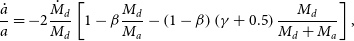 \begin{equation} \frac{\dot{a}}{a} = -2\frac{\dot{{M}}_{d}}{{{M}}_{d}}\left[1-\beta\frac{M_{d}}{M_{ a}}-\left(1-\beta\right)\left(\gamma+0.5\right)\frac{M_{d}}{M_{d}+M_{a}}\right],\end{equation}
where we can see that the change in the orbit’s semi-major axis during a mass transfer event depends on the masses of the components, the donor’s mass change rate, the accretion efficiency ( $\beta$
) and the location at which mass is being lost from the system (
$\beta$
) and the location at which mass is being lost from the system ( $\gamma$
).Footnote
b
$\gamma$
).Footnote
b
We also remark that even though we have focused in the effects of mass transfer accretion efficiency on orbital evolution, a non-zero value would result in mass gain for the accretor, which in turn has its evolution modified. See Hurley et al. (Reference Hurley, Pols and Tout2000) and Riley et al. (Reference Riley2022) for details.
2.1.5. Mass transfer stability
Once a star overflows its Roche lobe, whether the ensuing mass transfer is dynamically stable or not (leading to a CE event) is considered to depend on the response of both its radius and Roche lobe radius to mass loss (Paczyński & Sienkiewicz 1972; Hjellming & Webbink Reference Hjellming and Webbink1987; Soberman et al. Reference Soberman, Phinney and van den Heuvel1997). In compas, the default approach to evaluate this stability is to use the $\zeta$
prescription (e.g. Soberman et al. Reference Soberman, Phinney and van den Heuvel1997) as presented in section 4.2.2 of Riley et al. (Reference Riley2022). Additionally, we include the Ge et al. (Reference Ge, Webbink, Chen and Han2020) critical mass ratios (under the adiabatic assumption) as an alternative in order to test the effect of using a different, more recent prescription when evaluating the stability of a mass transfer event.
$\zeta$
prescription (e.g. Soberman et al. Reference Soberman, Phinney and van den Heuvel1997) as presented in section 4.2.2 of Riley et al. (Reference Riley2022). Additionally, we include the Ge et al. (Reference Ge, Webbink, Chen and Han2020) critical mass ratios (under the adiabatic assumption) as an alternative in order to test the effect of using a different, more recent prescription when evaluating the stability of a mass transfer event.
Evidently, we expect different mass transfer stability prescriptions to return different ratios of candidates being born from the stable mass transfer channel to the CE-related channels. This in turn should impact both the period distribution and number of mergers, whether they lead to an sdB candidate or not. Consequently, the total yield of sdBs would be modified as well.
Hertzsprung-Russell (top) and Kiel (bottom) diagram for HeMS evolutionary tracks of different mass values. Note that the Hurley et al. (Reference Hurley, Pols and Tout2000) models do not consider any hydrogen-rich outer layers, while the Bauer & Kupfer (Reference Bauer and Kupfer2021) models shown here consider a $10^{-3}$
M
$10^{-3}$
M $_\odot$
hydrogen-rich outer layer. The difference between stars that ignited helium in a flash (degenerate) and those that did it smoothly (non-degenerate) is noticeable.
$_\odot$
hydrogen-rich outer layer. The difference between stars that ignited helium in a flash (degenerate) and those that did it smoothly (non-degenerate) is noticeable.

2.2. Additional elements from MESA detailed models
2.2.1. Hydrogen-rich layer
The presence of an outer thin hydrogen-rich layer (see e.g. Brassard et al. Reference Brassard2001; Krzesinski et al. Reference Krzesinski, Blokesz, Baran and Bachulski2014; Hall & Jeffery Reference Hall and Jeffery2016, and references therein) in sdBs seems to play an important role as a regulator of both surface temperature and size, as depicted by figure 2 in H02, or figures 1 and 2 in Bauer & Kupfer (Reference Bauer and Kupfer2021). When there is little to no envelope, detailed stellar structure models show that a given sdB could be much more compact and hotter than a different sdB of similar mass possessing a $\sim$ $10^{-3}\,\mathrm{M}_\odot$
hydrogen-rich layer, a difference that would evidently affect observables such as surface gravity and effective temperature. This can be seen in Fig. 2 where
$10^{-3}\,\mathrm{M}_\odot$
hydrogen-rich layer, a difference that would evidently affect observables such as surface gravity and effective temperature. This can be seen in Fig. 2 where $\Delta T \sim 10\,000~K$
and
$\Delta T \sim 10\,000~K$
and $\Delta\log{g}\sim0.5$
in the most extreme cases.
$\Delta\log{g}\sim0.5$
in the most extreme cases.
The current stellar evolution prescription in compas, and most BPS codes that have adopted the Hurley et al. (Reference Hurley, Pols and Tout2000) scheme for stellar evolution, is limited to phases of naked helium stars only, which means that no hydrogen-rich envelopes have been considered for them. To get results closer to the observed sample of sdBs shown in Fig. 1, we adopt models built using mesa as presented in Bauer & Kupfer (Reference Bauer and Kupfer2021). These models include sdBs of masses below $0.58\,\mathrm{M}_\odot$
with (
$0.58\,\mathrm{M}_\odot$
with ( $10^{-3}$
or
$10^{-3}$
or $3\times10^{-3}\,\mathrm{M}_\odot$
) and without hydrogen-rich envelopes. We refer the reader to that work for technical details, as in this paper we focus solely on the prescription developed to incorporate their results into our sdB population synthesis scheme.
$3\times10^{-3}\,\mathrm{M}_\odot$
) and without hydrogen-rich envelopes. We refer the reader to that work for technical details, as in this paper we focus solely on the prescription developed to incorporate their results into our sdB population synthesis scheme.
To create a new rapid BPS-friendly prescription, we start by taking the same approach as Hurley et al. (Reference Hurley, Pols and Tout2000) and look for maximum sdB age (defined as the time spent core-helium burning) as a function of helium zero age main sequence (ZAHeMS) mass, which corresponds to the mass value as soon as the sdB progenitor has been stripped of most of its outer hydrogen-rich mass. Then, both radius and luminosity are taken as a function of relative age (time elapsed since ZAHeMS normalised by maximum age, that is, values between zero and one), hydrogen-rich shell mass and ZAHeMS mass. We note that, unlike models without hydrogen-rich shells, there is an additional dependence on the ZAMS mass of the progenitor: the models behave differently for stars with ZAMS below MHeF when compared to those above this critical mass limit, which ignite helium smoothly. An example of this behavior is shown in Fig. 2. This creates an additional challenge: since the value for MHeF changes between different stellar models and is affected by several parameters (e.g. metallicity, overshooting, and more; Cassisi Reference Cassisi, Lebreton, Valls-Gabaud and Charbonnel2014; Ghasemi et al. 2017), its exact value is not the same for Hurley et al. (Reference Hurley, Pols and Tout2000) and Bauer & Kupfer (Reference Bauer and Kupfer2021), showing that an ideal prescription for the evolution of HeMS stars with hydrogen-rich shells should also depend on the MHeF value predicted by the specific set of detailed models being analysed. Nonetheless, we proceed assuming that we can use the results presented in Bauer & Kupfer (Reference Bauer and Kupfer2021) without expanding the grid of models to account for the discrepancies, and apply them to the stars evolved through Hurley et al. (Reference Hurley, Pols and Tout2000) prescriptions as a first approach to the hydrogen envelope problem. However, we do consider the MHeF values computed following Hurley et al. (Reference Hurley, Pols and Tout2000) to decide whether we apply the prescription for the evolution of HeMS with hydrogen-rich shells predicted by the models that experience smooth helium ignition, or the one predicted by models that experience ignition in a flash instead.
After visual inspection of the different parameters involved in the models and attempting several different possible mathematical descriptions, we propose the following equations as a simplified prescription for the evolution of HeMS stars with hydrogen-rich shells:
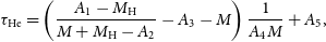 \begin{align} \tau_\textrm{He} = \left(\frac{A_1 - M_\textrm{H}}{M + M_\textrm{H} - A_2} - A_3 - M\right)\frac{1}{A_4 M} + A_5, \end{align}
 \begin{align} t_{r} = \frac{t}{\tau_\textrm{He}}, \end{align}
 \begin{align} R = B_1 + B_2t_{r} - \textrm{exp}\left(\left(1+M_\textrm{H}\right)\left(B_3+B_4t_{ r}\right)\right), \end{align}
 \begin{align} L = C_1(t_{r} + C_2) + C_3(t_{r} + C_4)^2 - 1\,000\frac{(t_{r} + C_5)^{10}}{1 + 25M_\textrm{H}} + \frac{1.5}{1 + C_6t_{r}},\end{align}
with $\tau_\textrm{He}$
the total time in Myr spent in the HeMS phaseFootnote
c
, t the time in Myr ellapsed since the ZAHeMS, M mass (no subscript indicates total mass, while an H subscript represents the hydrogen-rich shell mass), R radius and L luminosity. These last three elements are defined using solar units. The coefficients (
$\tau_\textrm{He}$
the total time in Myr spent in the HeMS phaseFootnote
c
, t the time in Myr ellapsed since the ZAHeMS, M mass (no subscript indicates total mass, while an H subscript represents the hydrogen-rich shell mass), R radius and L luminosity. These last three elements are defined using solar units. The coefficients ( $A_i, B_i, C_i$
with i a positive integer) were computed by making use of the scipy (Virtanen et al. Reference Virtanen2020) method curve_fit. Each of these coefficients is defined in Appendix B as a function of mass at ZAHeMS, mass at ZAMS, and hydrogen-rich shell mass. Overall, this prescription closely follows the stellar evolution predicted by the detailed models, as can be seen in Fig. B1.
$A_i, B_i, C_i$
with i a positive integer) were computed by making use of the scipy (Virtanen et al. Reference Virtanen2020) method curve_fit. Each of these coefficients is defined in Appendix B as a function of mass at ZAHeMS, mass at ZAMS, and hydrogen-rich shell mass. Overall, this prescription closely follows the stellar evolution predicted by the detailed models, as can be seen in Fig. B1.
As a final remark, we stress that this prescription is based on models constructed at solar metallicity, has not been tested for extrapolation (potentially generating results that are not reliable for parameters outside the range covered in Bauer & Kupfer Reference Bauer and Kupfer2021), and has not been directly incorporated into compas either. Consequently, all of the results shown in the following sections have been acquired through post-processing of the initial compas products.
2.2.2. Minimum core mass for helium ignition
An additional element to explore is the possibility of helium ignition while the helium core mass is still below the expected value at the tip of the RGB for stars with masses below MHeF, as explored in H02 (motivated by D’Cruz et al. Reference D’Cruz, Dorman, Rood and O’Connell1996). Inspired by the role that this parameter could potentially play in recovering the canonical mass distribution of sdBs and their birth rate, we use mesa to compare with the results presented in H02. We note, however, that the usage of different software and input physics generate noticeable differences between models (e.g. Ostrowski et al. Reference Ostrowski, Baran, Sanjayan and Sahoo2021). A clear example of this issue is shown in the top panel of Fig. 3.
The top panel shows how different methods predict the helium core mass ( $M_{c}$
) at helium ignition as a function of the mass at ZAMS, for models that experience a helium flash and have solar metallicity (defined as
$M_{c}$
) at helium ignition as a function of the mass at ZAMS, for models that experience a helium flash and have solar metallicity (defined as $Z = 0.02$
). Note that only the Bauer & Kupfer (Reference Bauer and Kupfer2021) models do not incorporate any overshooting prescription. On the bottom panel, a zoom-in of our mesa models (filled circles) is shown, alongside the minimum mass at which they were able to experience helium ignition (empty circles, explained in Section 2.2.2).
$Z = 0.02$
). Note that only the Bauer & Kupfer (Reference Bauer and Kupfer2021) models do not incorporate any overshooting prescription. On the bottom panel, a zoom-in of our mesa models (filled circles) is shown, alongside the minimum mass at which they were able to experience helium ignition (empty circles, explained in Section 2.2.2).
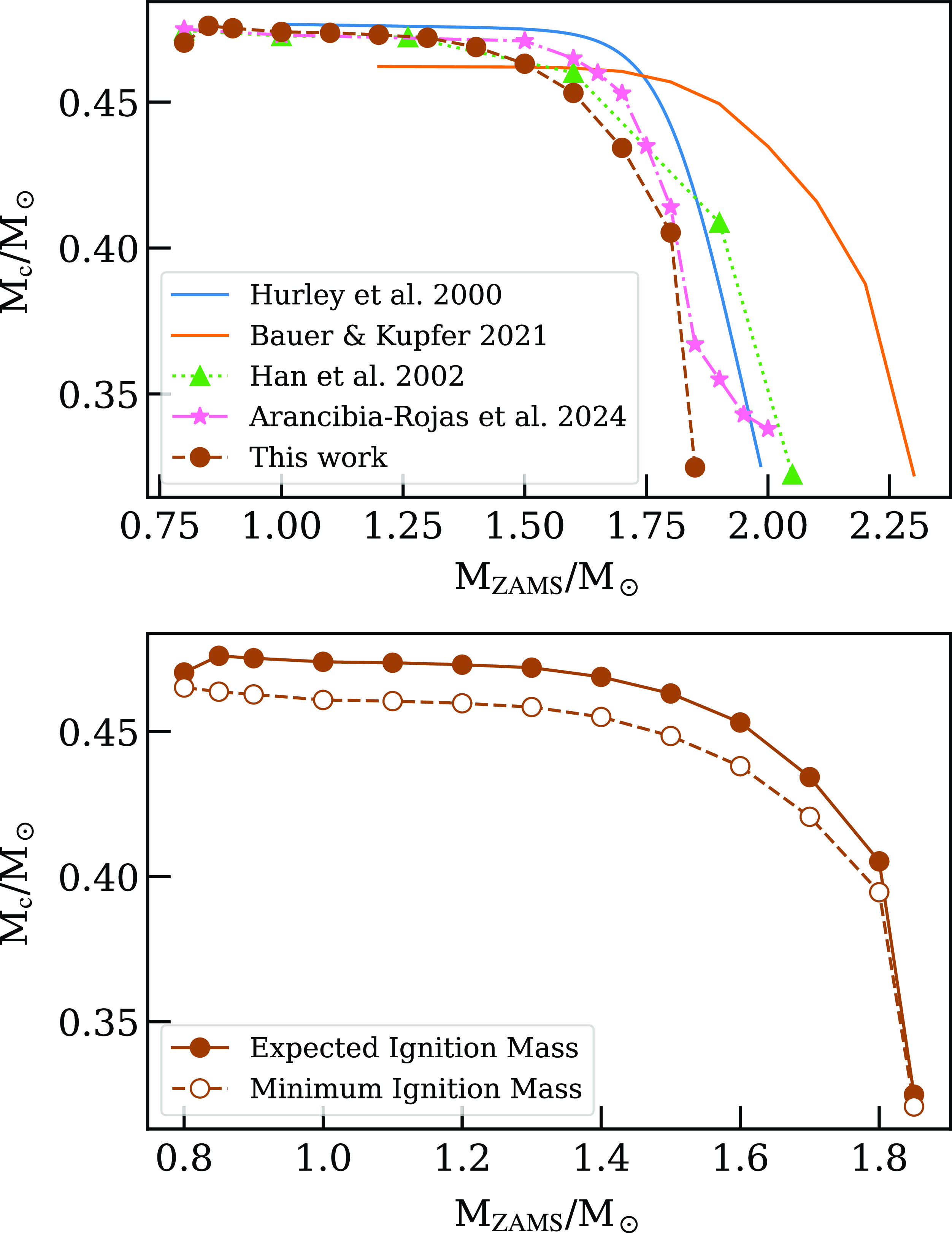
Our simplified approach consists of using mesa v21.12.1, specifically two modified versions of the included 1M_pre_ms_to_wd test suite: one in which evolution proceeds until right after helium is ignited in the core, from which we record the expected core mass at helium ignition; and another in which we stop evolution once the core has reached a given percent of the expected core mass at ignition, typically 95%. Afterwards, we artificially remove the envelope by relaxing the mass until only the helium core remains, at a mass loss rate given by $\dot{M} = 10^{-3} \frac{\mathrm{M}_\odot}{\mathrm{yr}}$
. Then, we let the star continue evolving until the core is cold enough (below 4 000 K, which implies evolution towards a helium white dwarf) or it ignites helium burning. By using a bisection method we can find the minimum percentage at which helium still ignites. Masses in the range of 0.8–1.85 M
$\dot{M} = 10^{-3} \frac{\mathrm{M}_\odot}{\mathrm{yr}}$
. Then, we let the star continue evolving until the core is cold enough (below 4 000 K, which implies evolution towards a helium white dwarf) or it ignites helium burning. By using a bisection method we can find the minimum percentage at which helium still ignites. Masses in the range of 0.8–1.85 M $_\odot$
were tested (Fig. 3, bottom panel), yielding an overall 3% difference from the expected core mass at the helium flash. This represents a 2% difference from typical 5% value found in H02.
$_\odot$
were tested (Fig. 3, bottom panel), yielding an overall 3% difference from the expected core mass at the helium flash. This represents a 2% difference from typical 5% value found in H02.
It is important to highlight that the percentage differences between H02 and our results can be increased or decreased by tuning the parameters of the model, so these discrepancies should not be considered to be conclusive on their own. Particularly, we neglected the hydrogen-rich shells, as we wanted to check what would the threshold be for naked helium stars, such as the ones that the Hurley et al. (Reference Hurley, Pols and Tout2000) prescription is based on. Additionally, in our implementation the parameters required for the mixing length and overshooting prescriptions (namely mixing_length_alpha and overshoot_f0) were not selected in order to minimise differences with H02, but computed through the solar simplex calibration included in mesa. We also note that our results could imply that the percentage differences are caused by a dependence of the minimum mass for helium ignition on the mass of the hydrogen-rich shell.
In a more detailed study, Arancibia-Rojas et al. (Reference Arancibia-Rojas2024) have recently explored the helium core mass ignition range for a higher number of initial masses and two different metallicity values (solar and subsolar), finding overall agreement with the 5% range presented in H02. An important difference, however, is that the 5% limit is relaxed for stars with progenitor masses above MHeF (those that ignite helium smoothly).
3. Results
3.1. Impact of parameter variations
The analysis in the following subsections is performed by taking the results from all 162 different configurations, and then dividing them in sub-groups that share characteristics in common. For example, when analyzing metallicity, 3 groups are found (subsolar, solar, and supersolar) and compared against each other. The overall number of sdB candidates from the 162 configurations corresponds to 486 425 systems, where only those binaries in which at least one member is classified as a HeMS star that falls within the selected space in the Kiel diagram (Fig. 1) has been considered. We also impose a cut on mass, limiting ourselves to sdB candidates with $M \leq 0.58~\mathrm{M}_\odot$
due to the constraints imposed by the range of masses covered by the Bauer & Kupfer (Reference Bauer and Kupfer2021) models. Although this affects the total number of systems that we recover, we note that candidates above this mass limit would quickly evolve and not spend much time as sdBs, as shown in Fig. 4 and also implied in both Yungelson (Reference Yungelson2008) and Arancibia-Rojas et al. (Reference Arancibia-Rojas2024). Similarly, their more massive progenitors (only smooth helium ignition can create such massive HeMS stars) correspond to rather low formation probabilities when compared to sdB candidates with masses below
$M \leq 0.58~\mathrm{M}_\odot$
due to the constraints imposed by the range of masses covered by the Bauer & Kupfer (Reference Bauer and Kupfer2021) models. Although this affects the total number of systems that we recover, we note that candidates above this mass limit would quickly evolve and not spend much time as sdBs, as shown in Fig. 4 and also implied in both Yungelson (Reference Yungelson2008) and Arancibia-Rojas et al. (Reference Arancibia-Rojas2024). Similarly, their more massive progenitors (only smooth helium ignition can create such massive HeMS stars) correspond to rather low formation probabilities when compared to sdB candidates with masses below $\sim$ $0.5~\mathrm{M}_\odot$
that are born from progenitors with masses under MHeF, due to the initial mass function.
$0.5~\mathrm{M}_\odot$
that are born from progenitors with masses under MHeF, due to the initial mass function.
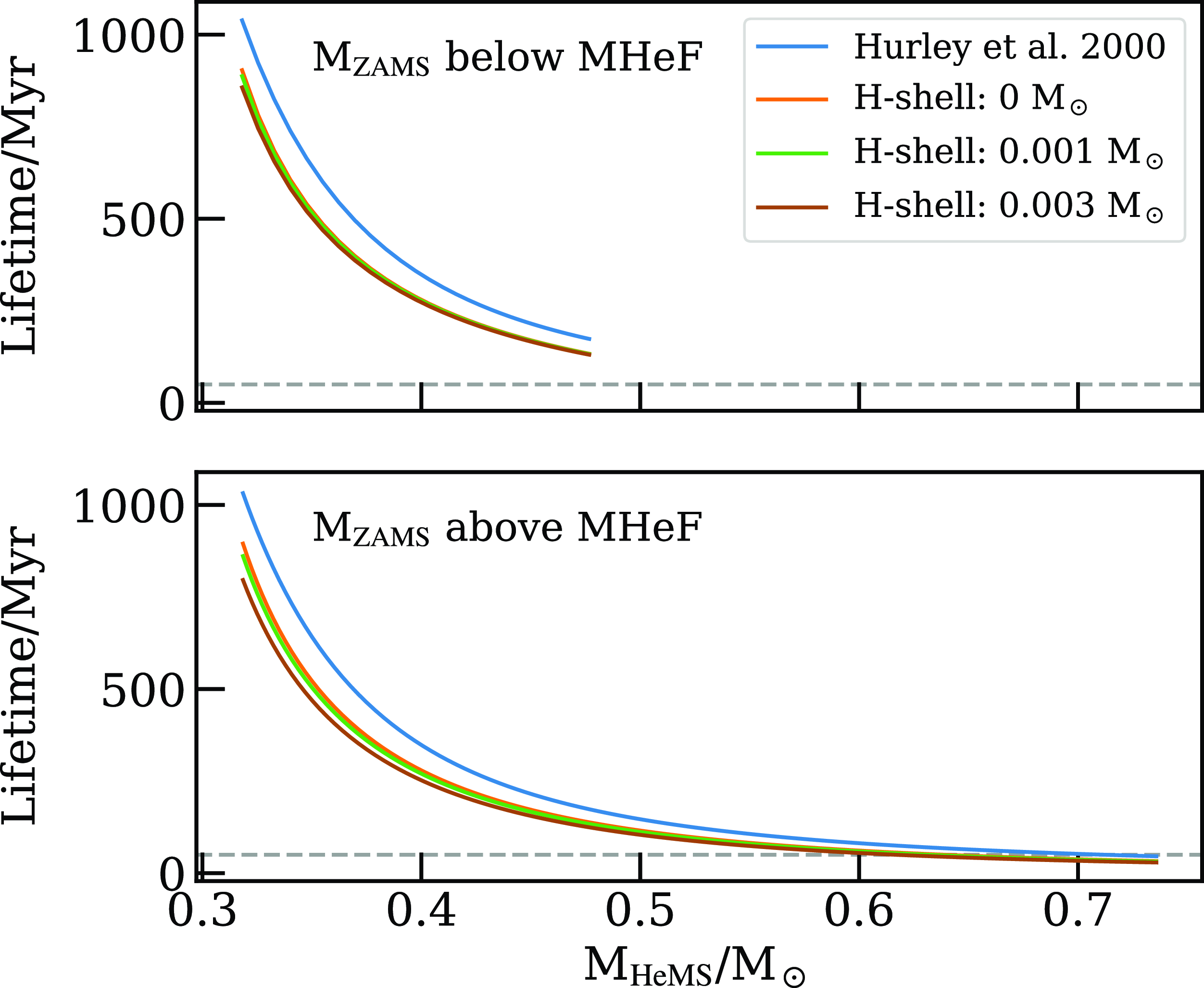
Maximum time spent as a HeMS star as a function of mass. The top panel shows stars that experience a flash at helium ignition, while the bottom panel depicts the smooth ignition scenario. The horizontal dashed line shows a lifetime equal 50 Myr, highlighting that candidates with masses above $\sim\!0.58\,\textrm{M}_\odot$
spend a comparatively short time as HeMS stars.
$\sim\!0.58\,\textrm{M}_\odot$
spend a comparatively short time as HeMS stars.
3.1.1. Common envelope: The $\alpha$
efficiency parameter
$\alpha$
efficiency parameter

The analysis of this parameter only includes systems that have experienced at least one CE event, as otherwise changes in $\alpha$
would have no impact on the binary stellar population. By considering its definition from Equation (5), we expect lower
$\alpha$
would have no impact on the binary stellar population. By considering its definition from Equation (5), we expect lower $\alpha$
values to result in less systems surviving CE episodes due to more frequent mergers within the population, as the higher amount of orbital energy required to eject the envelope of the potential HeMS progenitor star would result in smaller separations after the CE. This can be seen in Fig. 5, where we show all systems that have undergone at least one CE episode before becoming a HeMS star. As expected, lower alpha values result in fewer systems becoming HeMS, with the total number of the
$\alpha$
values to result in less systems surviving CE episodes due to more frequent mergers within the population, as the higher amount of orbital energy required to eject the envelope of the potential HeMS progenitor star would result in smaller separations after the CE. This can be seen in Fig. 5, where we show all systems that have undergone at least one CE episode before becoming a HeMS star. As expected, lower alpha values result in fewer systems becoming HeMS, with the total number of the $\alpha = 0.2$
configuration being about 13
$\alpha = 0.2$
configuration being about 13 $\%$
of the number of systems found for
$\%$
of the number of systems found for $\alpha = 1.5$
. Despite the differences in total numbers, most systems that evolve up to the HeMS stage through any channel involving at least one CE episode are typically found in short period systems, below
$\alpha = 1.5$
. Despite the differences in total numbers, most systems that evolve up to the HeMS stage through any channel involving at least one CE episode are typically found in short period systems, below $\sim$
10 days and peaking between 0.1–1 days in the logarithmic period distribution. An exception to this property is seen for
$\sim$
10 days and peaking between 0.1–1 days in the logarithmic period distribution. An exception to this property is seen for $\alpha = 0.2$
, due to the low efficiency and consequent higher amount of orbital energy spent in removing the envelope of the sdB progenitor, resulting in more compact orbits and a peak below 0.1 days in the logarithmic period distribution. This effect also explains the slight differences in the location of the logarithmic period distribution peak for the remaining
$\alpha = 0.2$
, due to the low efficiency and consequent higher amount of orbital energy spent in removing the envelope of the sdB progenitor, resulting in more compact orbits and a peak below 0.1 days in the logarithmic period distribution. This effect also explains the slight differences in the location of the logarithmic period distribution peak for the remaining $\alpha$
values. We also note that long period systems are found in these CE channels, though most of them can be understood as systems that experienced a CE episode at an early evolutionary stage, and therefore was not the direct precursor of the HeMS star. A latter stable mass transfer would then form the sdB candidate and also increase the orbital separation.
$\alpha$
values. We also note that long period systems are found in these CE channels, though most of them can be understood as systems that experienced a CE episode at an early evolutionary stage, and therefore was not the direct precursor of the HeMS star. A latter stable mass transfer would then form the sdB candidate and also increase the orbital separation.
Top row, from left to right: Number of candidates per logarithmic-period bin, ZAMS mass distribution, and ratio of candidates being born from the initially primary star to the initially secondary star. Bottom row, from left to right: Stellar type of the progenitor and stellar type of the companion at the primary’s ZAHeMS stage (stellar types are defined in Table 2). Note that we present sub-samples grouped by $\alpha$
value, in order to highlight the effects of modifying this parameter. The blue, orange and green histograms correspond to
$\alpha$
value, in order to highlight the effects of modifying this parameter. The blue, orange and green histograms correspond to $\alpha$
values equal to 0.2, 1.0, and 1.5, respectively. Only systems that have experienced at least one CE episode are shown.
$\alpha$
values equal to 0.2, 1.0, and 1.5, respectively. Only systems that have experienced at least one CE episode are shown.
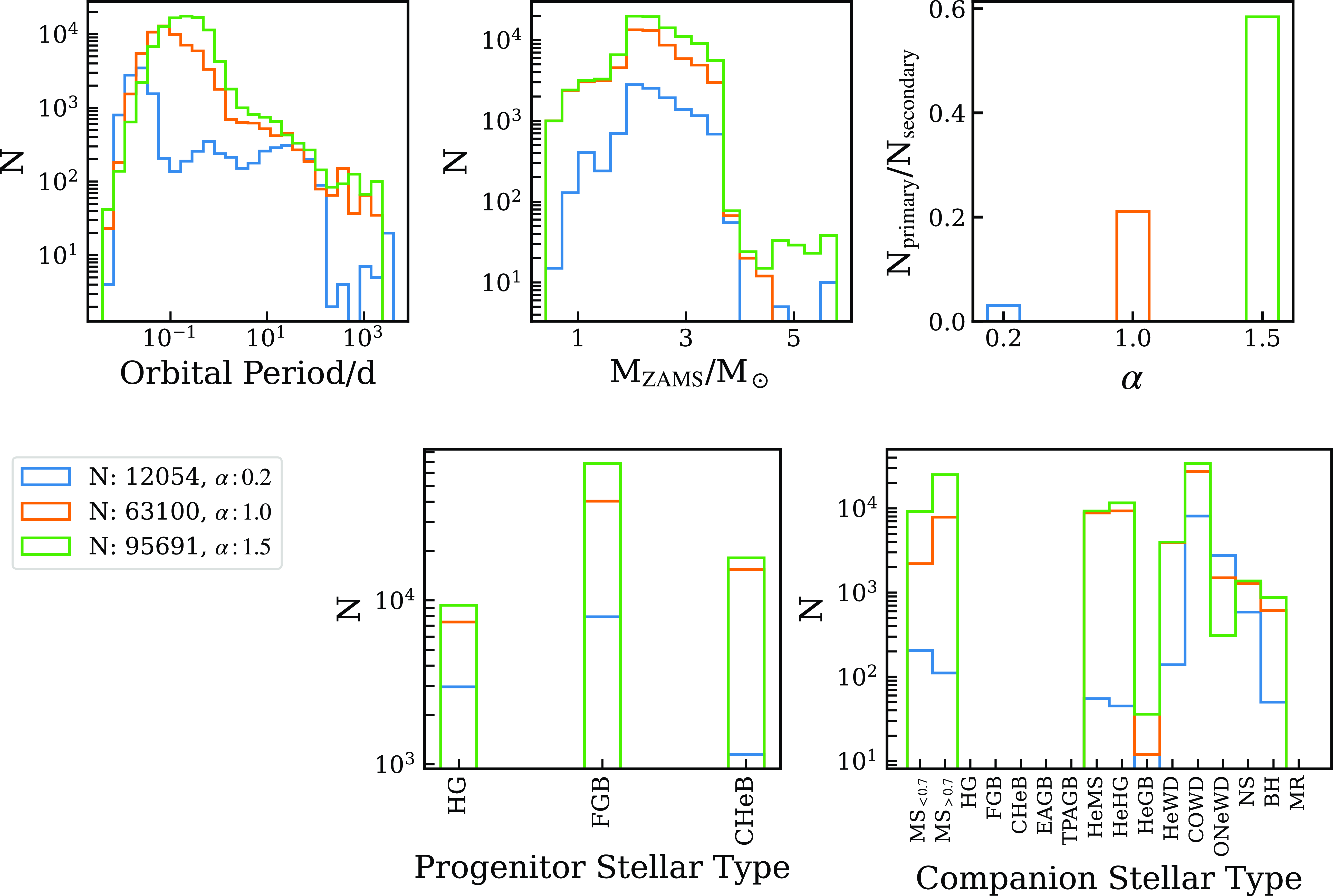
Interestingly, the increasing number of candidates for higher $\alpha$
values seems to be linked to progenitors with ZAMS masses above MHeF that eventually evolve into HeMS stars. As for the companions of our candidates, there are no clear trends linked to the changing
$\alpha$
values seems to be linked to progenitors with ZAMS masses above MHeF that eventually evolve into HeMS stars. As for the companions of our candidates, there are no clear trends linked to the changing $\alpha$
values, all stellar types increase with increasing
$\alpha$
values, all stellar types increase with increasing $\alpha$
. Perhaps the only exception would be the number of ONeWD companions, which show the highest value for
$\alpha$
. Perhaps the only exception would be the number of ONeWD companions, which show the highest value for $\alpha = 0.2$
. The ratio of this number against the number of COWD companions might shed some light on the CE process.
$\alpha = 0.2$
. The ratio of this number against the number of COWD companions might shed some light on the CE process.
Other interesting features are the ratio of initially primaries to initially secondaries that become sdB candidates, and the progenitor stellar type. The ratio shows an increasing value with $\alpha$
: low
$\alpha$
: low $\alpha$
favours initial secondaries becoming candidates (the opposite is true for high
$\alpha$
favours initial secondaries becoming candidates (the opposite is true for high $\alpha$
), potentially because only those systems where the initially primary star quickly evolves to the WD stage can remove the envelope of the secondary during a CE without merging; while the progenitor stellar type shows a preference for FGB stars with HG (CHeB) as second option for low (high)
$\alpha$
), potentially because only those systems where the initially primary star quickly evolves to the WD stage can remove the envelope of the secondary during a CE without merging; while the progenitor stellar type shows a preference for FGB stars with HG (CHeB) as second option for low (high) $\alpha$
.
$\alpha$
.
3.1.2. Metallicity changes
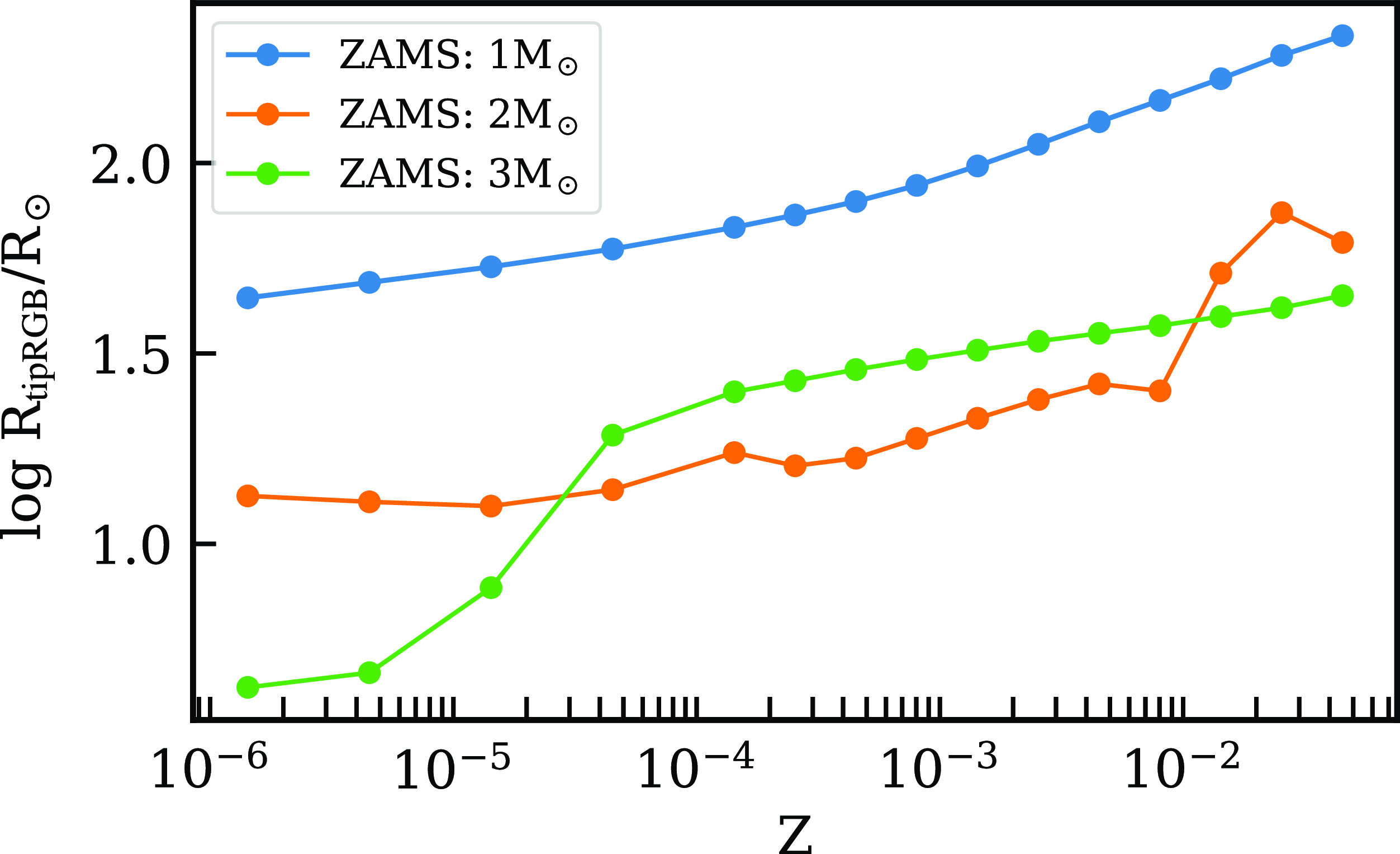
As mentioned in Section 2.1.3, metallicity is expected to play a role in a few different settings. The helium core mass and the size of the star at the tip of the RGB should both depend on the chosen metallicity value and, similarly, metallicity plays a role in defining the MHeF critical mass limit for degenerate or smooth helium ignition. Indeed, some of these effects can be seen in results for detailed models, such as what can be found in the mist stellar evolutionary tracks (Choi et al. Reference Choi2016), explicitly shown in Fig. 6.
Dependence of the stellar radius at the tip of the RGB on metallicity, as shown by the evolutionary tracks from the mist grids (Choi et al. Reference Choi2016). We have chosen tracks that were computed and not interpolated, extracted metallicity values from the stored Zinit property, and interpreted the radius at tip of the RGB as the last (age-wise) radius value for which the corresponding time step is classified as having a phase equal to 2 (values equal to 2 consider both the sub-giant and red giant phase, see Choi et al. Reference Choi2016 for details).
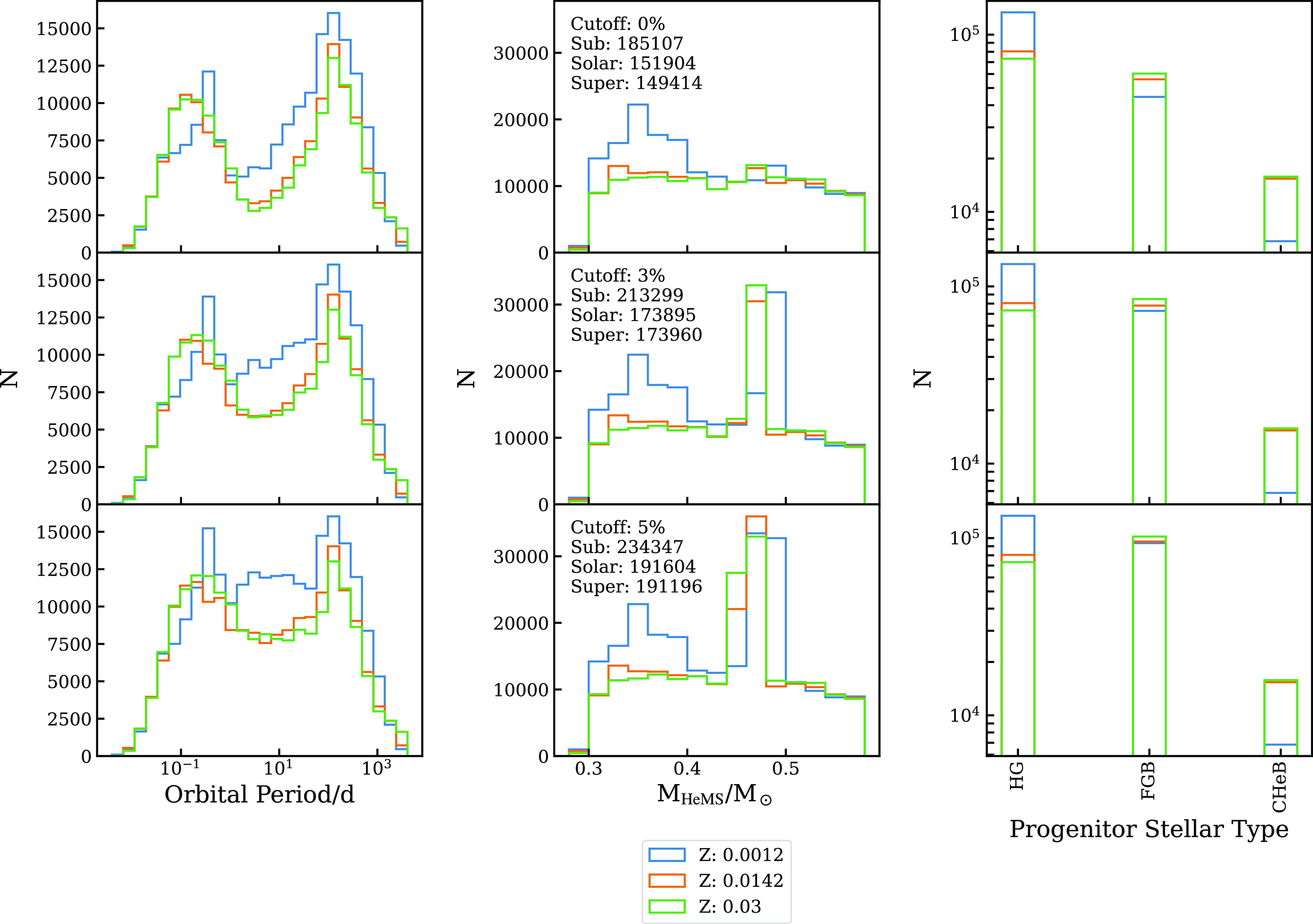
As an overview of the effect of metallicity on our populations, we can say that there is a decrease in the total number of candidates with increasing metallicity (the number of candidates per metallicity are shown in the left-hand side column of Fig. 7). Taking the analysis one step further, within the top panels of Fig. 7 we compare grids that share the same configuration but vary their metallicity value, and we can see that most of the stars that no longer become sdB candidates at higher metallicities are those that evolve from HG progenitors. These stars usually result in sdBs with masses below $\sim$ $0.43\,\textrm{M}_\odot$
, meaning that they must have evolved from progenitors with masses close to the MHeF limit (Fig. 3). It can also be seen that the canonical mass peak, around
$0.43\,\textrm{M}_\odot$
, meaning that they must have evolved from progenitors with masses close to the MHeF limit (Fig. 3). It can also be seen that the canonical mass peak, around $\sim$ $0.47\textrm{ M}_\odot$
, is displaced towards higher masses at lower metallicities, while the peak located at short orbital periods (
$0.47\textrm{ M}_\odot$
, is displaced towards higher masses at lower metallicities, while the peak located at short orbital periods ( $\lesssim$
1 day) is slightly displaced towards longer periods. Within the same period distribution, a gap forms between 1–10 days, which becomes more pronounced for higher metallicity values. The gap is less evident for larger values of the threshold for helium ignition (Section 3.1.5), but the trend with metallicity remains. We note that beyond slight differences in the total number of sdB candidates, there are not many remarkable differences between our supersolar and solar metallicity population, most likely due to the rather small 2.1 multiplicative factor required to scale our solar value to the supersolar one. This contrasts with our subsolar metallicity value, where the required factor is 0.08.
$\lesssim$
1 day) is slightly displaced towards longer periods. Within the same period distribution, a gap forms between 1–10 days, which becomes more pronounced for higher metallicity values. The gap is less evident for larger values of the threshold for helium ignition (Section 3.1.5), but the trend with metallicity remains. We note that beyond slight differences in the total number of sdB candidates, there are not many remarkable differences between our supersolar and solar metallicity population, most likely due to the rather small 2.1 multiplicative factor required to scale our solar value to the supersolar one. This contrasts with our subsolar metallicity value, where the required factor is 0.08.
From left to right: changes in orbital period, mass at HeMS and progenitor stellar type for our sdB candidates. The cutoff for stars that ignite helium in the core increases from top to bottom as a percent difference: 0%, 3%, and 5%. This can be understood as follows: the top panel shows candidates who have a mass equal or higher than the helium core mass expected at the tip of the RGB, while subsequent rows show the impact of considering HeWDs within 3% and 5% of this expected core mass as sdB progenitors. Different colors show different metallicities as indicated by the legend, with blue being sub-solar ( ${Z} = 0.0012$
), orange solar (
${Z} = 0.0012$
), orange solar ( ${Z} = 0.0142$
), and green super-solar (
${Z} = 0.0142$
), and green super-solar ( ${Z} = 0.03$
). See Sections 3.1.2 and 3.1.5 for details.
${Z} = 0.03$
). See Sections 3.1.2 and 3.1.5 for details.
3.1.3. Mass lost from the system
Equation (14) shows the interplay between mass being transferred from the donor to the accretor and what fraction is kept in the latter. In cases where the mass is not completely retained, the equation also takes into account the location at which this mass is being lost from the system and establishes the amount of specific angular momentum lost. These properties are encoded by $\beta$
and
$\beta$
and $\gamma$
’s definition, as shown in Equations (13) and (12), respectively. However, it is not straightforward to predict the final effect of Equation (14) for the orbit, due to its non-linear dependence on the
$\gamma$
’s definition, as shown in Equations (13) and (12), respectively. However, it is not straightforward to predict the final effect of Equation (14) for the orbit, due to its non-linear dependence on the $\beta$
and
$\beta$
and $\gamma$
parameters, the mass of each component, and the mass loss rate of the donor. Instead, we can perform a simple analysis of Equation (14) to estimate whether the rate of change of the semi-major axis will be negative or positive (the orbital separation shrinks or grows) after a mass transfer episode. First, the factor outside the square brackets on the right-hand side of Equation (14) is always
$\gamma$
parameters, the mass of each component, and the mass loss rate of the donor. Instead, we can perform a simple analysis of Equation (14) to estimate whether the rate of change of the semi-major axis will be negative or positive (the orbital separation shrinks or grows) after a mass transfer episode. First, the factor outside the square brackets on the right-hand side of Equation (14) is always $\geq$
0, considering the minus sign and that mass is being lost from the donor (its mass change rate is negative). Then, we define a mass ratio
$\geq$
0, considering the minus sign and that mass is being lost from the donor (its mass change rate is negative). Then, we define a mass ratio $q = { M}_{a}/{M}_{d}$
and analyse the sign of the expression within the square brackets in Equation (14), referenced as
$q = { M}_{a}/{M}_{d}$
and analyse the sign of the expression within the square brackets in Equation (14), referenced as $\phi$
hereafter. We can see that:
$\phi$
hereafter. We can see that:
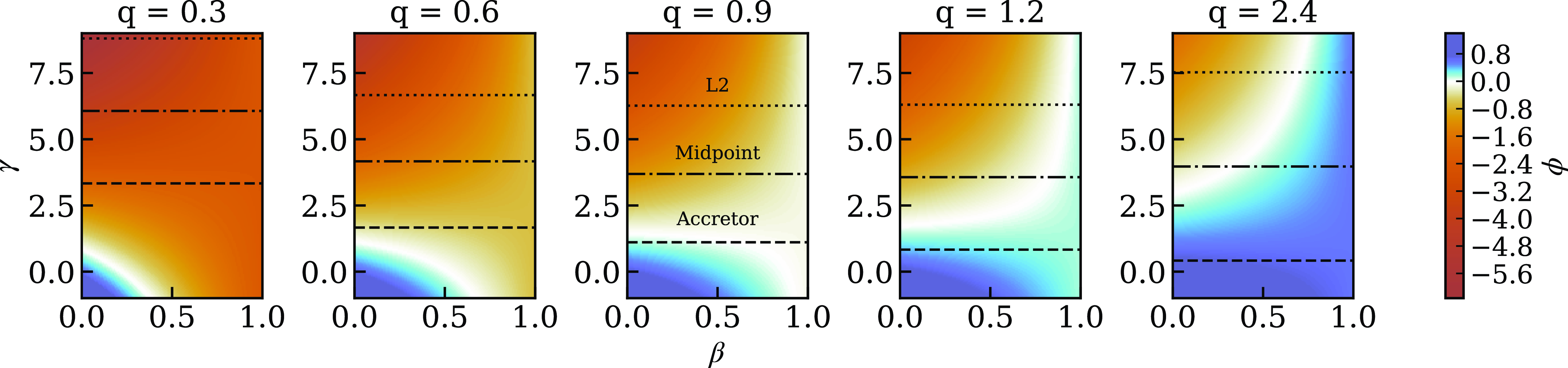
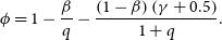 \begin{align} \phi = 1-\frac{\beta}{q}-\frac{\left(1-\beta\right)\left(\gamma+0.5\right)}{1+q}. \end{align}
A visualization that helps to understand the values that $\phi$
can take is shown in Fig. 8, where it can be seen that for most of the configurations being shown
$\phi$
can take is shown in Fig. 8, where it can be seen that for most of the configurations being shown $\phi$
is negative and, as a consequence, the orbital separation should shrink. This trend is reversed as we progress into the mass ratio reversal regime (q becomes greater than 1). It should be noted that for this analysis we have assumed that
$\phi$
is negative and, as a consequence, the orbital separation should shrink. This trend is reversed as we progress into the mass ratio reversal regime (q becomes greater than 1). It should be noted that for this analysis we have assumed that $\gamma$
is equal to the upper limit shown in Willcox et al. (Reference Willcox, MacLeod, Mandel and Hirai2023) when MLF is equal to 1. Accordingly,
$\gamma$
is equal to the upper limit shown in Willcox et al. (Reference Willcox, MacLeod, Mandel and Hirai2023) when MLF is equal to 1. Accordingly, $\gamma$
takes the value
$\gamma$
takes the value $1/q$
when mass is lost from the position of the accretor, implying that MLF is equal to 0. MLF equal to 0.5 follows from the previous two definitions, as the intermediate value.
$1/q$
when mass is lost from the position of the accretor, implying that MLF is equal to 0. MLF equal to 0.5 follows from the previous two definitions, as the intermediate value.
Contour plots of $\phi$
as a function of
$\phi$
as a function of $\beta$
and
$\beta$
and $\gamma$
, for a given mass ratio (q). Representative values of
$\gamma$
, for a given mass ratio (q). Representative values of $\gamma$
are shown for reference, depending on where mass is being lost from the system: the dotted line corresponds to L2, the dashed line to the position of the accretor, and the dash-dotted line to the midpoint between the previous two. The more positive (bluer)
$\gamma$
are shown for reference, depending on where mass is being lost from the system: the dotted line corresponds to L2, the dashed line to the position of the accretor, and the dash-dotted line to the midpoint between the previous two. The more positive (bluer) $\phi$
is, the more the orbital separation grows. The opposite is true for negative (orange) values. For details, see Section 3.1.3.
$\phi$
is, the more the orbital separation grows. The opposite is true for negative (orange) values. For details, see Section 3.1.3.
To analyse the impact of changing $\beta$
and
$\beta$
and $\gamma$
in our different compas populations, we present Figs. 9 and 10, which depict how some physical properties change when keeping
$\gamma$
in our different compas populations, we present Figs. 9 and 10, which depict how some physical properties change when keeping $\beta$
constant and varying
$\beta$
constant and varying $\gamma$
, and vice versa. Before proceeding with the analysis, however, it must be noted that the mass accretion efficiency parameter in compas only affects stable mass transfer episodes. Unstable mass transfer always results in no mass accreted in compas
Footnote
d
(Riley et al. Reference Riley2022).
$\gamma$
, and vice versa. Before proceeding with the analysis, however, it must be noted that the mass accretion efficiency parameter in compas only affects stable mass transfer episodes. Unstable mass transfer always results in no mass accreted in compas
Footnote
d
(Riley et al. Reference Riley2022).
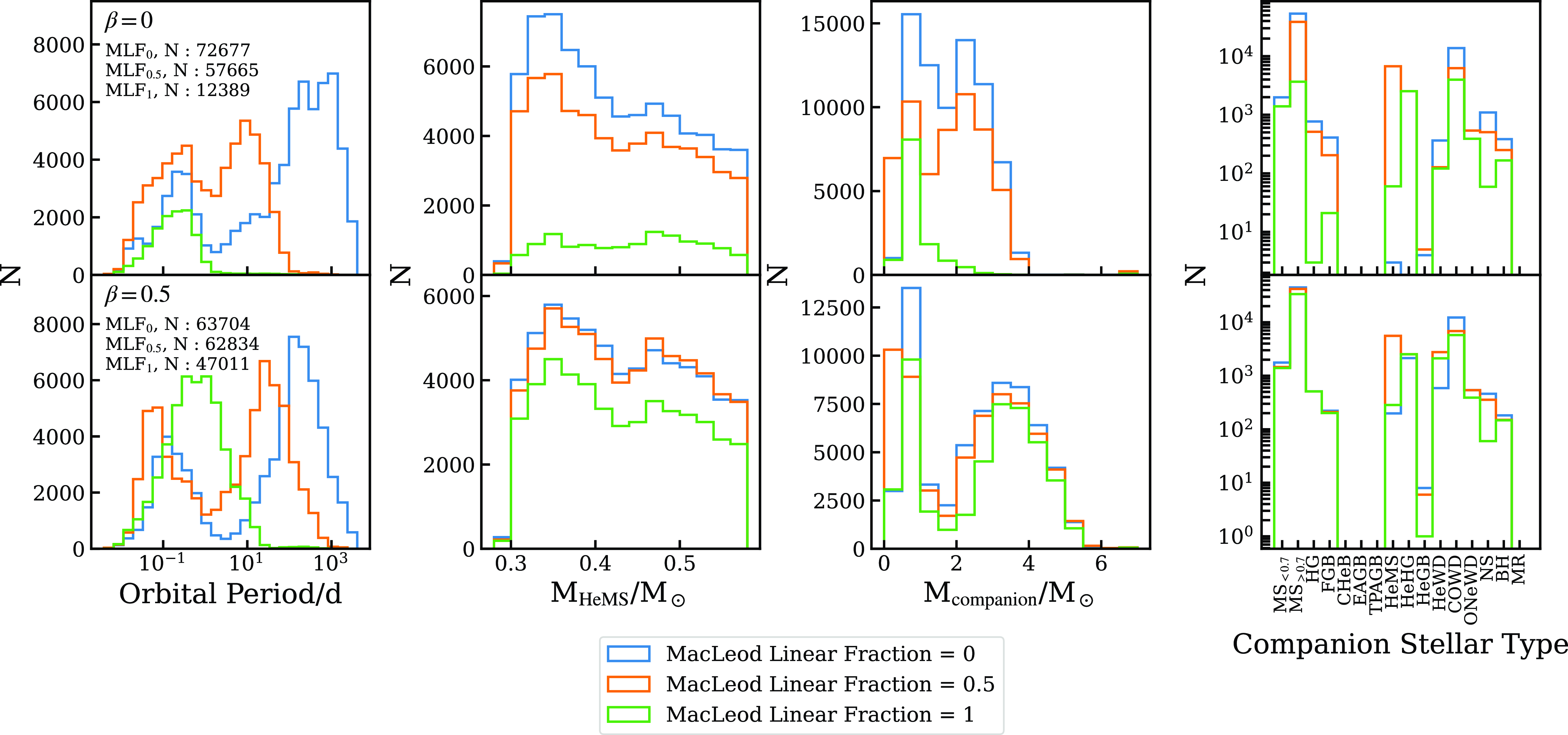
Graphical analysis of the impact of changing the MLF at a constant $\beta$
value. From top to bottom:
$\beta$
value. From top to bottom: $\beta = 0$
and
$\beta = 0$
and $\beta = 0.5$
. From left to right: Orbital period, mass of the candidate at the start of the HeMS, companion’s mass at the start of the HeMS, and companion stellar type at the same evolutionary stage. Different colours indicate different values for the MLF, with the number of candidates per configuration being specified within the text of the left-hand side panels.
$\beta = 0.5$
. From left to right: Orbital period, mass of the candidate at the start of the HeMS, companion’s mass at the start of the HeMS, and companion stellar type at the same evolutionary stage. Different colours indicate different values for the MLF, with the number of candidates per configuration being specified within the text of the left-hand side panels.
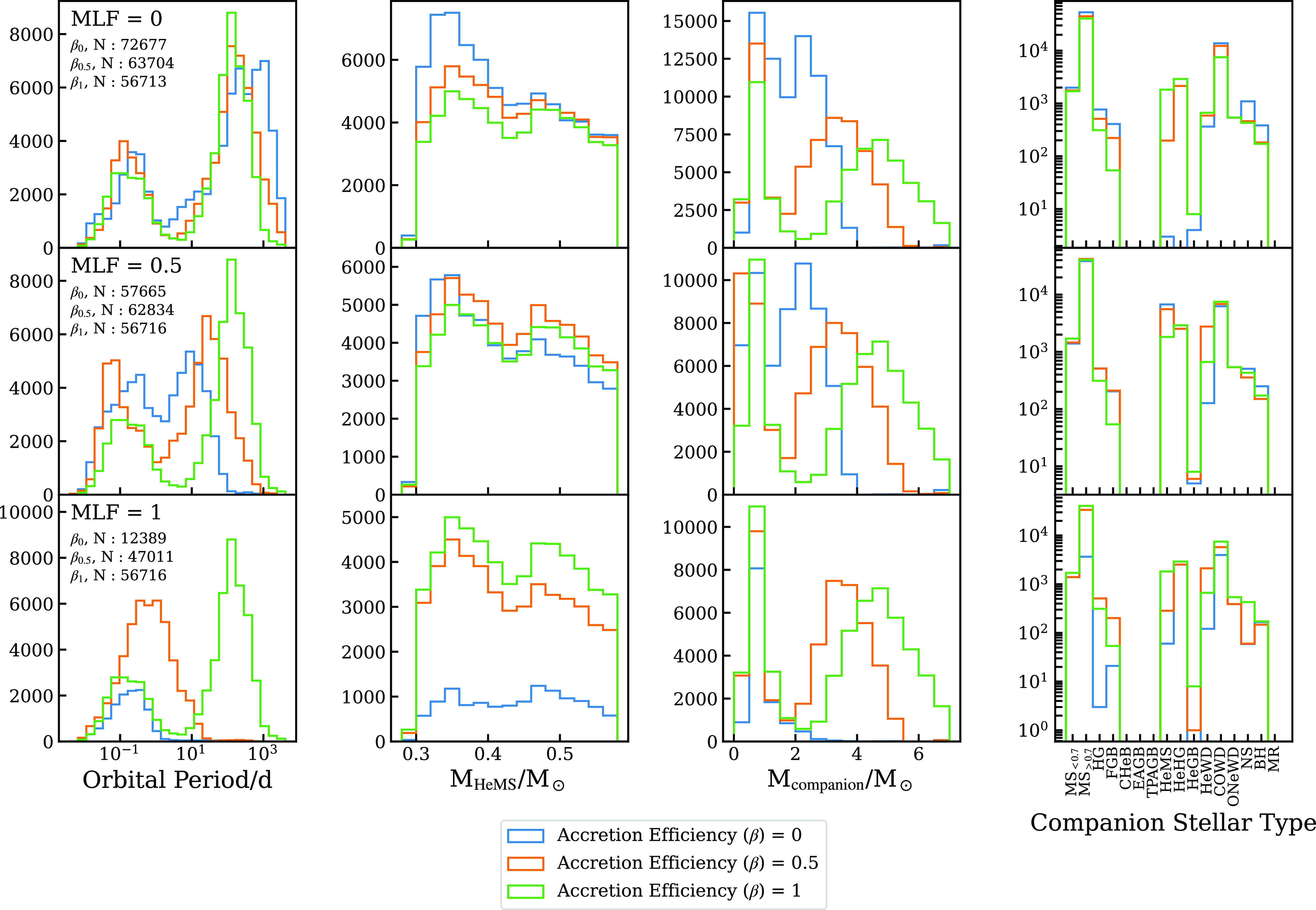
Similar to Fig. 9, graphical analysis of the impact of changing the Accretion Efficiency ( $\beta$
) at a constant MLF value. From top to bottom:
$\beta$
) at a constant MLF value. From top to bottom: $\textrm{MLF} = 0$
,
$\textrm{MLF} = 0$
, $\textrm{MLF} = 0.5$
and
$\textrm{MLF} = 0.5$
and $\textrm{MLF} = 1$
. From left to right: Orbital period, mass of the candidate at the ZAHeMS, companion mass at the ZAHeMS, and companion stellar type at the same evolutionary stage. Different colours indicate different values for
$\textrm{MLF} = 1$
. From left to right: Orbital period, mass of the candidate at the ZAHeMS, companion mass at the ZAHeMS, and companion stellar type at the same evolutionary stage. Different colours indicate different values for $\beta$
, with the number of candidates per configuration being specified within the text inside the left-hand side panels.
$\beta$
, with the number of candidates per configuration being specified within the text inside the left-hand side panels.
In the case of keeping $\beta$
equal to zero and varying
$\beta$
equal to zero and varying $\gamma$
(top panels in Fig. 9), we note that the number of candidates drops as we increase the latter (in the form of MLF), which can be understood as fewer systems surviving in closer orbits due to the impact of
$\gamma$
(top panels in Fig. 9), we note that the number of candidates drops as we increase the latter (in the form of MLF), which can be understood as fewer systems surviving in closer orbits due to the impact of $\phi$
continuously decreasing. This can be seen in Fig. 8 where
$\phi$
continuously decreasing. This can be seen in Fig. 8 where $\phi$
becomes increasingly negative for
$\phi$
becomes increasingly negative for $q \lesssim 0.9$
as MLF (
$q \lesssim 0.9$
as MLF ( $\gamma$
) increases. A similar trend is present for higher values of q, though in these cases the lowest MLF values start at
$\gamma$
) increases. A similar trend is present for higher values of q, though in these cases the lowest MLF values start at $\phi \gtrsim 0$
and transition into negative values as MLF grows. Overall, this results in many systems from the top panel in Fig. 9 either merging or following different evolutionary paths as a consequence of the increase on MLF: the long period peak at about 1 000 days when MLF equals 0 is shifted towards 10 days when MLF increases by 0.5, and the new peak is not as tall. This effect is further strengthened by losing mass from L2 instead (MLF
$\phi \gtrsim 0$
and transition into negative values as MLF grows. Overall, this results in many systems from the top panel in Fig. 9 either merging or following different evolutionary paths as a consequence of the increase on MLF: the long period peak at about 1 000 days when MLF equals 0 is shifted towards 10 days when MLF increases by 0.5, and the new peak is not as tall. This effect is further strengthened by losing mass from L2 instead (MLF $ = 1$
), which results in a single peak below 1 day. Regarding the mass distribution, it seems to have a common pattern with two peaks, no matter the value of
$ = 1$
), which results in a single peak below 1 day. Regarding the mass distribution, it seems to have a common pattern with two peaks, no matter the value of $\gamma$
, though it can be noted that the low-mass peak is comparatively higher than the peak around the canonical (
$\gamma$
, though it can be noted that the low-mass peak is comparatively higher than the peak around the canonical ( $\sim$ $0.47$
M
$0.47$
M $_\odot$
) mass for the MLF
$_\odot$
) mass for the MLF $ \lt 1$
scenarios. This difference is smaller for increasing
$ \lt 1$
scenarios. This difference is smaller for increasing $\gamma$
values, and shows a reversal in peak prominence when MLF
$\gamma$
values, and shows a reversal in peak prominence when MLF $ = 1$
, a trend that can be linked to a preference for progenitors with masses around the MHeF limit when MLF takes values lower than 1. As for the characteristics of the companions, their mass distributions peak at
$ = 1$
, a trend that can be linked to a preference for progenitors with masses around the MHeF limit when MLF takes values lower than 1. As for the characteristics of the companions, their mass distributions peak at $\sim$
1 M
$\sim$
1 M $_\odot$
independent of the MLF choice, though a secondary peak can be observed at about 2 M
$_\odot$
independent of the MLF choice, though a secondary peak can be observed at about 2 M $_\odot$
. This additional peak is of similar relevance to the low mass one when MLF
$_\odot$
. This additional peak is of similar relevance to the low mass one when MLF $=0.5$
, but completely vanishes for MLF
$=0.5$
, but completely vanishes for MLF $=1$
. Overall, both peaks decrease with increasing MLF value. These changes seem to be driven by a drop in the number of companions in stages of evolution earlier than the FGB.
$=1$
. Overall, both peaks decrease with increasing MLF value. These changes seem to be driven by a drop in the number of companions in stages of evolution earlier than the FGB.
When looking at a constant 0.5 value for $\beta$
(bottom panels in Fig. 9), a similar analysis can be made. The number of candidates also decreases as we increase
$\beta$
(bottom panels in Fig. 9), a similar analysis can be made. The number of candidates also decreases as we increase $\gamma$
, but the differences become smaller and are almost negligible between MLF equal to 0 and 0.5. This can be seen in Fig. 8, as the colour corresponding to
$\gamma$
, but the differences become smaller and are almost negligible between MLF equal to 0 and 0.5. This can be seen in Fig. 8, as the colour corresponding to $\phi$
values does not change as much as in the case of
$\phi$
values does not change as much as in the case of $\beta = 0$
(for increasing
$\beta = 0$
(for increasing $\gamma$
). By looking at the significance of the long period and short period peak at each MLF value shown in the period distribution, it can be seen that smaller MLF values favour longer periods since
$\gamma$
). By looking at the significance of the long period and short period peak at each MLF value shown in the period distribution, it can be seen that smaller MLF values favour longer periods since $\phi$
is closer to 0 as q grows, and it can take positive values once
$\phi$
is closer to 0 as q grows, and it can take positive values once $q \gtrsim 1$
. However, the displacement of each peak does not follow a clear dependence on MLF, unless the single peak present for MLF
$q \gtrsim 1$
. However, the displacement of each peak does not follow a clear dependence on MLF, unless the single peak present for MLF $= 1$
corresponds to the long period peak of the other two MLF values, in which case it would have been shifted enough to merge with the short period peak, implying closer orbits for larger MLF values overall. The mass distribution shows a similar pattern to that observed when
$= 1$
corresponds to the long period peak of the other two MLF values, in which case it would have been shifted enough to merge with the short period peak, implying closer orbits for larger MLF values overall. The mass distribution shows a similar pattern to that observed when $\beta$
is equal to 0, though the relative significance of the two peaks (at about 0.35 M
$\beta$
is equal to 0, though the relative significance of the two peaks (at about 0.35 M $_\odot$
and canonical mass) is rather constant. Additionally, the number of systems for MLF
$_\odot$
and canonical mass) is rather constant. Additionally, the number of systems for MLF $= 1$
is much higher than in the
$= 1$
is much higher than in the $\beta = 0$
scenario. Finally, the companions show two peaks in their mass distribution, one in the 0–1 M
$\beta = 0$
scenario. Finally, the companions show two peaks in their mass distribution, one in the 0–1 M $_\odot$
mass range and another at about 3.5 M
$_\odot$
mass range and another at about 3.5 M $_\odot$
. Both decrease their prominence with increasing MLF values.
$_\odot$
. Both decrease their prominence with increasing MLF values.
The case of constant $\beta = 1$
is not analysed as changes in
$\beta = 1$
is not analysed as changes in $\gamma$
would not impact the distributions. This can be understood through either Equation (14) or (19), since they show that setting full accretion efficiency implies that there would be no mass being lost from the system that could carry a fraction of angular momentum away during a mass transfer event.
$\gamma$
would not impact the distributions. This can be understood through either Equation (14) or (19), since they show that setting full accretion efficiency implies that there would be no mass being lost from the system that could carry a fraction of angular momentum away during a mass transfer event.
We can also probe the effects of different mass retention efficiencies ( $\beta$
) by keeping MLF constant in a similar fashion to what was done before, though the analysis this time requires considering Fig. 10 instead.
$\beta$
) by keeping MLF constant in a similar fashion to what was done before, though the analysis this time requires considering Fig. 10 instead.
When losing mass from the accretor’s position (MLF = 0), there is a clear preference for periods longer than $\sim$
100 days, though we notice that there is a slight dependence of the number of candidates on the value of
$\sim$
100 days, though we notice that there is a slight dependence of the number of candidates on the value of $\beta$
, as they decrease with increasing
$\beta$
, as they decrease with increasing $\beta$
. This results in period and mass distributions without striking differences between configurations. The biggest differences between
$\beta$
. This results in period and mass distributions without striking differences between configurations. The biggest differences between $\beta = 0$
and the other configurations are the number of candidates in both intermediate (
$\beta = 0$
and the other configurations are the number of candidates in both intermediate ( $\sim$
1–10 days) and long (
$\sim$
1–10 days) and long ( $\sim$
1 000 days) periods, or low-mass sdBs that peak at
$\sim$
1 000 days) periods, or low-mass sdBs that peak at $\sim$ $0.35\,\textrm{M}_\odot$
in the mass distribution. Another expected characteristic is that a larger
$0.35\,\textrm{M}_\odot$
in the mass distribution. Another expected characteristic is that a larger $\beta$
value results in more massive companions due to larger masses being retained, as can be observed in the displacement of the secondary peak towards higher mass values in the companion mass distribution with increasing
$\beta$
value results in more massive companions due to larger masses being retained, as can be observed in the displacement of the secondary peak towards higher mass values in the companion mass distribution with increasing $\beta$
.
$\beta$
.
Similar to Figs. 9 and 10, each panel from left to right corresponds to orbital period, mass of the candidate at ZAHeMS, mass of the companion at ZAHeMS, and the companion’s stellar type at the same stage. In this case, different critical mass ratio prescriptions are being tested: in blue, the $\zeta$
prescription labeled as NONE due to how it is implemented in compas and, in orange, the Ge et al. (Reference Ge, Webbink, Chen and Han2020) prescription (see Section 2.1.5 for details).
$\zeta$
prescription labeled as NONE due to how it is implemented in compas and, in orange, the Ge et al. (Reference Ge, Webbink, Chen and Han2020) prescription (see Section 2.1.5 for details).
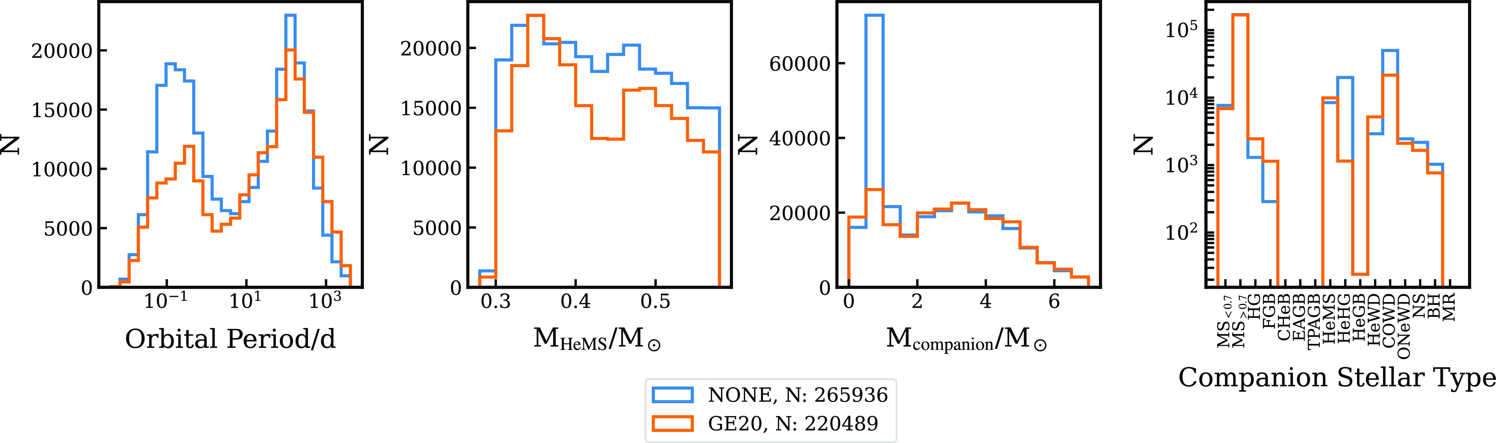
Instead, if every system is set to lose mass from an intermediate location between the accretor and L2 (MLF = 0.5), the changes on the number of candidates between the different accretion efficiency values are even smaller than in the MLF $=0$
case, and there is no clear preference for long-period systems anymore. Despite this, the differences between different choices of
$=0$
case, and there is no clear preference for long-period systems anymore. Despite this, the differences between different choices of $\beta$
are clearer in the distributions. We can see two peaks that have a similar significance when
$\beta$
are clearer in the distributions. We can see two peaks that have a similar significance when $\beta = 0$
, and progressively show a more relevant long period peak with increasing
$\beta = 0$
, and progressively show a more relevant long period peak with increasing $\beta$
. Along this trend, the long period peak is also shifted to longer periods, from an initial peak about 10 days (when there is no accretion), up to
$\beta$
. Along this trend, the long period peak is also shifted to longer periods, from an initial peak about 10 days (when there is no accretion), up to $\gtrsim$
100 days when there is full accretion. This can be associated to less angular momentum being carried away by mass lost from the system during mass transfer events for higher values of
$\gtrsim$
100 days when there is full accretion. This can be associated to less angular momentum being carried away by mass lost from the system during mass transfer events for higher values of $\beta$
and, as a consequence, orbits not shrinking as much. However, the HeMS mass distribution seems to have the same set of features, independent of the choice of
$\beta$
and, as a consequence, orbits not shrinking as much. However, the HeMS mass distribution seems to have the same set of features, independent of the choice of $\beta$
. Of course, the frequency per bin changes depending on the total number of candidates, but the presence of two peaks (
$\beta$
. Of course, the frequency per bin changes depending on the total number of candidates, but the presence of two peaks ( $\sim$
0.35 M
$\sim$
0.35 M $_\odot$
and around canonical mass) remains unaltered. There seems to be a slight dependence on relative peak prominence with accretion efficiency, though: higher
$_\odot$
and around canonical mass) remains unaltered. There seems to be a slight dependence on relative peak prominence with accretion efficiency, though: higher $\beta$
values create peaks of increasingly similar height. The companion mass distribution is rather similar to the MLF
$\beta$
values create peaks of increasingly similar height. The companion mass distribution is rather similar to the MLF $ = 0$
case, as we can notice that higher accretion efficiency values result in more massive companions (shown by the displacement of the secondary peak towards higher masses).
$ = 0$
case, as we can notice that higher accretion efficiency values result in more massive companions (shown by the displacement of the secondary peak towards higher masses).
Finally, by setting MLF = 1, we find the biggest changes in the number of candidates per accretion efficiency configuration, as $\beta = 0$
yields around 20% of the total number of candidates that can be obtained by setting
$\beta = 0$
yields around 20% of the total number of candidates that can be obtained by setting $\beta = 1$
instead. It is worth noting that an interesting behavior can be observed in the period distribution: if we consider the
$\beta = 1$
instead. It is worth noting that an interesting behavior can be observed in the period distribution: if we consider the $\beta = 0$
case as the base configuration, then increasing the accretion efficiency up to a 0.5 value creates more short and intermediate period systems (up to
$\beta = 0$
case as the base configuration, then increasing the accretion efficiency up to a 0.5 value creates more short and intermediate period systems (up to $\sim$
10 days) and keeps the distribution as a single peaked one. This changes in the full accretion efficiency case (
$\sim$
10 days) and keeps the distribution as a single peaked one. This changes in the full accretion efficiency case ( $\beta = 1$
), since an additional long period peak can be found, but the short period peak is almost equal to the base scenario. This is most likely another form of the patterns seen in the bottom panel of Fig. 9 and discussed earlier in the text, though in this case the long period peak at full accretion is displaced to shorter periods at
$\beta = 1$
), since an additional long period peak can be found, but the short period peak is almost equal to the base scenario. This is most likely another form of the patterns seen in the bottom panel of Fig. 9 and discussed earlier in the text, though in this case the long period peak at full accretion is displaced to shorter periods at $\beta = 0.5$
, giving the impression of a single peak. Many systems composing this peak are unable to generate sdB candidates when there is no accretion, hence the much smaller (and single) peak in this case. The mass distribution of the candidates follows the same pattern as in the previous MLF configurations, except for the case without accretion which breaks the trend and shows a much flatter distribution. Interestingly, the mass distribution of the companions does not show a relevant number of massive
$\beta = 0.5$
, giving the impression of a single peak. Many systems composing this peak are unable to generate sdB candidates when there is no accretion, hence the much smaller (and single) peak in this case. The mass distribution of the candidates follows the same pattern as in the previous MLF configurations, except for the case without accretion which breaks the trend and shows a much flatter distribution. Interestingly, the mass distribution of the companions does not show a relevant number of massive $\gtrsim$
2 M
$\gtrsim$
2 M $_\odot$
companions for the case without accretion.
$_\odot$
companions for the case without accretion.
3.1.4. Mass transfer stability prescription
As the name indicates, the choice for mass transfer stability prescription determines whether a star experiences a stable or unstable mass transfer episode after filling its Roche lobe. This, in turn, affects the number of sdB candidates and their characteristics, as can be seen in Fig. 11. In rough numbers, the $\zeta$
prescription (e.g. Soberman et al. Reference Soberman, Phinney and van den Heuvel1997, labeled as NONE in Fig. 11) produces around 1.2 times more candidates than the GE20 (Ge et al. Reference Ge, Webbink, Chen and Han2020) prescription, though these differences are concentrated around channels involving CE events: the NONE prescription yields 1.6 and 2.5 times more candidates than the GE20 one for 1 and 2 CE episodes pre-candidate formation, respectively. Moreover, if analysed in detail, the overall number of candidates is not the only difference. First, GE20 seems to prefer long period systems. This is not the case for the
$\zeta$
prescription (e.g. Soberman et al. Reference Soberman, Phinney and van den Heuvel1997, labeled as NONE in Fig. 11) produces around 1.2 times more candidates than the GE20 (Ge et al. Reference Ge, Webbink, Chen and Han2020) prescription, though these differences are concentrated around channels involving CE events: the NONE prescription yields 1.6 and 2.5 times more candidates than the GE20 one for 1 and 2 CE episodes pre-candidate formation, respectively. Moreover, if analysed in detail, the overall number of candidates is not the only difference. First, GE20 seems to prefer long period systems. This is not the case for the $\zeta$
prescription, as the preference for long orbital periods is not so evident and the relative significance of both long and short period peaks is similar. Similarly, the mass distribution of sdB candidates seems to decay almost linearly in the case of the
$\zeta$
prescription, as the preference for long orbital periods is not so evident and the relative significance of both long and short period peaks is similar. Similarly, the mass distribution of sdB candidates seems to decay almost linearly in the case of the $\zeta$
prescription, but has two clear peaks if the GE20 distribution is considered instead.
$\zeta$
prescription, but has two clear peaks if the GE20 distribution is considered instead.
The properties of the companions also depend on the chosen mass transfer stability prescription. It is clear that the GE20 prescription yields less systems overall, linked to the $\zeta$
prescription allowing the existence of a sharp and tall peak at
$\zeta$
prescription allowing the existence of a sharp and tall peak at $\sim$
0.7 M
$\sim$
0.7 M $_\odot$
companion masses. This also indicates differences in the stellar types of the companions, confirmed by the right-hand side panel of Fig. 11: the
$_\odot$
companion masses. This also indicates differences in the stellar types of the companions, confirmed by the right-hand side panel of Fig. 11: the $\zeta$
prescription generates a higher number of COWDs as well as HeHG companions.
$\zeta$
prescription generates a higher number of COWDs as well as HeHG companions.
3.1.5. Ignition below the expected core mass
As stated in Section 2.2.2, the analysis of our sdB candidates requires considering the possibility of stars igniting helium burning when their core mass is below the expected value near the tip of the RGB. We have tackled this issue by collecting stars originally classified as helium white dwarfs (HeWDs) and used their mass values as input for our new HeMS with hydrogen-rich shells prescription, which returns evolutionary tracks as if they were HeMS stars instead. We only consider HeWDs that are within the mass cutoff of either 3 or 5% that we set based on results from Section 2.2.2 and previous studies (Han et al. Reference Han, Podsiadlowski, Maxted, Marsh and Ivanova2002; Arancibia-Rojas et al. Reference Arancibia-Rojas2024). While it is possible to follow a similar approach to Zorotovic & Schreiber (Reference Zorotovic and Schreiber2013) and use the actual values found for minimum helium ignition mass in either Han et al. (Reference Han, Podsiadlowski, Maxted, Marsh and Ivanova2002) or Arancibia-Rojas et al. (Reference Arancibia-Rojas2024), we note that both studies present a $\sim$
5% threshold for stars igniting helium in a flash, independent of the chosen metallicity value, hence our choice of 5% for one of the tested configurations. The case of more massive progenitors that ignite helium smoothly is slightly more complicated, as according to Arancibia-Rojas et al. (Reference Arancibia-Rojas2024) there is a wider range of masses for ignition (their tables B1 and B2). On top of that, the width of this range also depends on the ZAMS mass of the model: there is a linear increase from 5% at ZAMS masses corresponding to the most massive progenitors that ignite helium in a flash, up to
$\sim$
5% threshold for stars igniting helium in a flash, independent of the chosen metallicity value, hence our choice of 5% for one of the tested configurations. The case of more massive progenitors that ignite helium smoothly is slightly more complicated, as according to Arancibia-Rojas et al. (Reference Arancibia-Rojas2024) there is a wider range of masses for ignition (their tables B1 and B2). On top of that, the width of this range also depends on the ZAMS mass of the model: there is a linear increase from 5% at ZAMS masses corresponding to the most massive progenitors that ignite helium in a flash, up to $\sim$
30% at about 3 M
$\sim$
30% at about 3 M $_\odot$
. This value then decreases at a slower rate (it is
$_\odot$
. This value then decreases at a slower rate (it is $\sim$
15% at 6M
$\sim$
15% at 6M $_\odot$
), but the trend is nonetheless completely different from the relatively flat 5% value for models igniting helium in a flash. For simplicity purposes, and noting that the realization probability of more massive progenitors is much lower due to the initial mass function (IMF), we decide to use flat threshold values. The impact of these different threshold values on our population can be seen in Fig. 7, where a considerable spike in the number of candidates around canonical mass can be observed for cutoff values
$_\odot$
), but the trend is nonetheless completely different from the relatively flat 5% value for models igniting helium in a flash. For simplicity purposes, and noting that the realization probability of more massive progenitors is much lower due to the initial mass function (IMF), we decide to use flat threshold values. The impact of these different threshold values on our population can be seen in Fig. 7, where a considerable spike in the number of candidates around canonical mass can be observed for cutoff values $ \gt $
0%, independent of the chosen value for metallicity (histograms of different colours). As expected, increasing the percentage for the mass cutoff increases the total amount of candidates, though interestingly this increase is focused on stars with masses around the canonical sdB mass value (
$ \gt $
0%, independent of the chosen value for metallicity (histograms of different colours). As expected, increasing the percentage for the mass cutoff increases the total amount of candidates, though interestingly this increase is focused on stars with masses around the canonical sdB mass value ( $\sim$
0.47 M
$\sim$
0.47 M $_\odot$
) and intermediate orbital periods between
$_\odot$
) and intermediate orbital periods between $\sim$
1–10 days only. It can be inferred that the observational sdB sample and its mass distribution would be directly impacted by the real value of the mass cutoff, though additional constraints such as the delay times associated to the formation of these objects play a non-negligible role. Additionally, it is possible to see that the peak in the mass distribution is shifted depending on the chosen value for metallicity, as a consequence of the arguments discussed in Section 3.1.2.
$\sim$
1–10 days only. It can be inferred that the observational sdB sample and its mass distribution would be directly impacted by the real value of the mass cutoff, though additional constraints such as the delay times associated to the formation of these objects play a non-negligible role. Additionally, it is possible to see that the peak in the mass distribution is shifted depending on the chosen value for metallicity, as a consequence of the arguments discussed in Section 3.1.2.
We remark that this is a simple approach to the underlying question of the lower limit for helium ignition and it represents a first order estimate. As previously mentioned, the results from Arancibia-Rojas et al. (Reference Arancibia-Rojas2024) show that stars with ZAMS mass above the MHeF mass limit require a broken linear function with different slopes for mass values above/below $\sim$
3 M
$\sim$
3 M $_\odot$
, though in a Galaxy-like sampling these systems would not be as common due to the IMF.
$_\odot$
, though in a Galaxy-like sampling these systems would not be as common due to the IMF.
3.1.6. Hydrogen-rich shell mass
The definition of HeMS stars in the Hurley et al. (Reference Hurley, Pols and Tout2000) scheme adopted by compas implies a complete absence of any hydrogen-rich envelope, due to the prescription for their evolution being based on detailed models of ZAHeMS stars ( $Y = 0.98$
and
$Y = 0.98$
and $Z = 0.02$
composition). Although this is a useful simplification in the context of rapid BPS codes, it yields estimates for effective temperature and surface gravity that are different from observations (e.g. Fig. 12, upper panel). Indeed, the absence of any external hydrogen-rich shells makes the candidates from simulations cluster at high temperature and surface gravity, unlike the spread of the observed distribution. The inclusion of hydrogen-rich shells through the prescription based on Bauer & Kupfer (Reference Bauer and Kupfer2021) and developed in Section 2.2.1 seems to properly address the issue and yields results that improve the agreement with observables, as can be seen in the bottom panel of Fig. 12. As one might intuitively expect, the more massive the envelope is, the less compact and colder a star can become. This effect can be seen through the location and coverage of each patch within the figure and, although the coverage is not perfect, we must keep in mind that the current state of the prescription is limited in mass range as well as envelope size (see Section 2.2.1). This lack of coverage at lower surface gravity and temperature in Fig. 12 suggests that higher mass envelopes are needed and will be addressed in future work.
$Z = 0.02$
composition). Although this is a useful simplification in the context of rapid BPS codes, it yields estimates for effective temperature and surface gravity that are different from observations (e.g. Fig. 12, upper panel). Indeed, the absence of any external hydrogen-rich shells makes the candidates from simulations cluster at high temperature and surface gravity, unlike the spread of the observed distribution. The inclusion of hydrogen-rich shells through the prescription based on Bauer & Kupfer (Reference Bauer and Kupfer2021) and developed in Section 2.2.1 seems to properly address the issue and yields results that improve the agreement with observables, as can be seen in the bottom panel of Fig. 12. As one might intuitively expect, the more massive the envelope is, the less compact and colder a star can become. This effect can be seen through the location and coverage of each patch within the figure and, although the coverage is not perfect, we must keep in mind that the current state of the prescription is limited in mass range as well as envelope size (see Section 2.2.1). This lack of coverage at lower surface gravity and temperature in Fig. 12 suggests that higher mass envelopes are needed and will be addressed in future work.
Comparison between the physical properties of the compas sample when no hydrogen-rich outer layers are considered (top panel) and when they are included by using the prescription presented in Section 2.2.1 (bottom). This last element is further explored by presenting the area covered by the compas sdB candidates depending on their M $_\textrm{H}$
value, which corresponds to the hydrogen-rich outer envelope’s mass (in Solar mass units). Scatter points (in blue) are taken from the Culpan et al. (Reference Culpan2022) observational sample and shown for reference.
$_\textrm{H}$
value, which corresponds to the hydrogen-rich outer envelope’s mass (in Solar mass units). Scatter points (in blue) are taken from the Culpan et al. (Reference Culpan2022) observational sample and shown for reference.
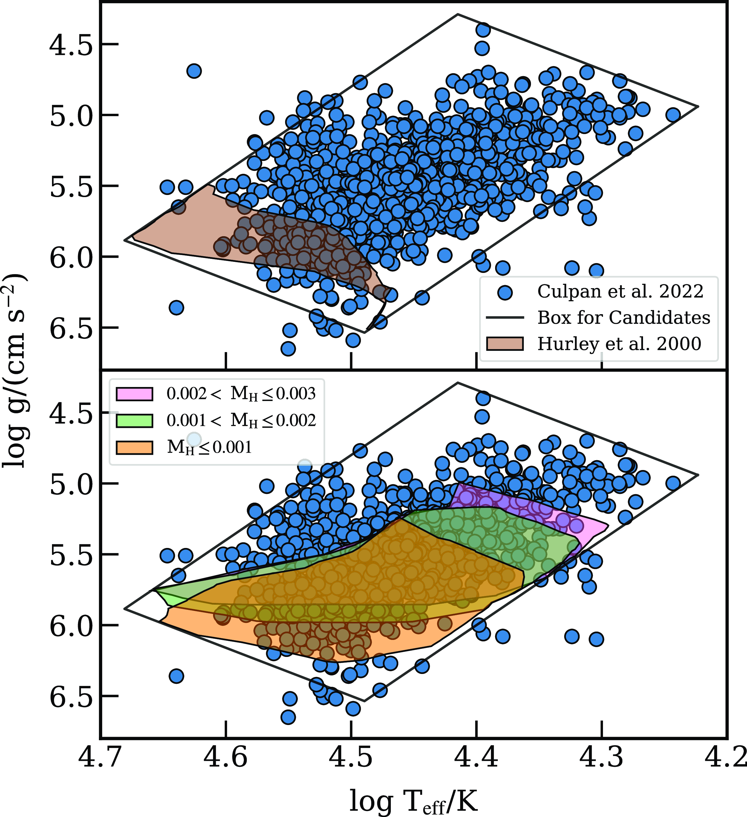
It is important to note that the impact on the total number of sdB candidates is almost negligible, as the inclusion of hydrogen-rich shells only increase the number of sdB candidates by 1%. Also, these hydrogen-rich envelopes do not affect the orbital evolution of the systems. After the onset of a mass transfer episode, the external low-density hydrogen-rich shell would be slowly transferred during a few tens of mega-years, while the orbit shrinks due to gravitational wave radiation (see Bauer & Kupfer Reference Bauer and Kupfer2021, section 3.1).
Finally, an important question left to answer is related to the mass distribution of these hydrogen-rich envelopes. The different sdB formation channels involve different interactions and progenitors at different evolutionary stages, which would potentially impact the preferred size of the hydrogen-rich layers (as previously noted in H02). We made no special assumptions and limited ourselves to randomly sampling masses in the range 0 to $3\times10^{-3} \textrm{M}_\odot$
, which corresponds to the values covered by the Bauer & Kupfer (Reference Bauer and Kupfer2021) models.
$3\times10^{-3} \textrm{M}_\odot$
, which corresponds to the values covered by the Bauer & Kupfer (Reference Bauer and Kupfer2021) models.
Different sdB formation channels found in our compas chosen model. From left to right, columns contain the orbital period, the stellar mass on the ZAHeMS, total time it takes to form an sdB candidate, mass distribution of the companions, and the stellar type of the companion when the candidate starts the HeMS. From top to bottom, we show an increasing number of CE events that led to the candidate’s formation: No CE episodes (stable mass transfer only), one CE episode and two common envelope episodes. To highlight different companion types, we have used different shades: the lightest shade corresponds to Stellar Type $ \gt 9$
(white dwarfs, neutron stars, or black holes), while the darkest shade corresponds to Stellar Type
$ \gt 9$
(white dwarfs, neutron stars, or black holes), while the darkest shade corresponds to Stellar Type $= 0$
(MS companions with masses
$= 0$
(MS companions with masses $\leq$
0.7 M
$\leq$
0.7 M $_\odot$
). A white colour indicates types in-between (check Table 2 for definitions, though most of these companions correspond to MS stars with masses
$_\odot$
). A white colour indicates types in-between (check Table 2 for definitions, though most of these companions correspond to MS stars with masses $ \gt $
0.7 M
$ \gt $
0.7 M $_\odot$
), and the sum of the contribution of each one of these 3 colours corresponds to the total amount of systems in a given bin. A hatched yellow area has been used to highlight candidates evolving through the ECE+RLOF channel, defined in Section 3.2.2. Note that in each panel the y-axis has a different range.
$_\odot$
), and the sum of the contribution of each one of these 3 colours corresponds to the total amount of systems in a given bin. A hatched yellow area has been used to highlight candidates evolving through the ECE+RLOF channel, defined in Section 3.2.2. Note that in each panel the y-axis has a different range.
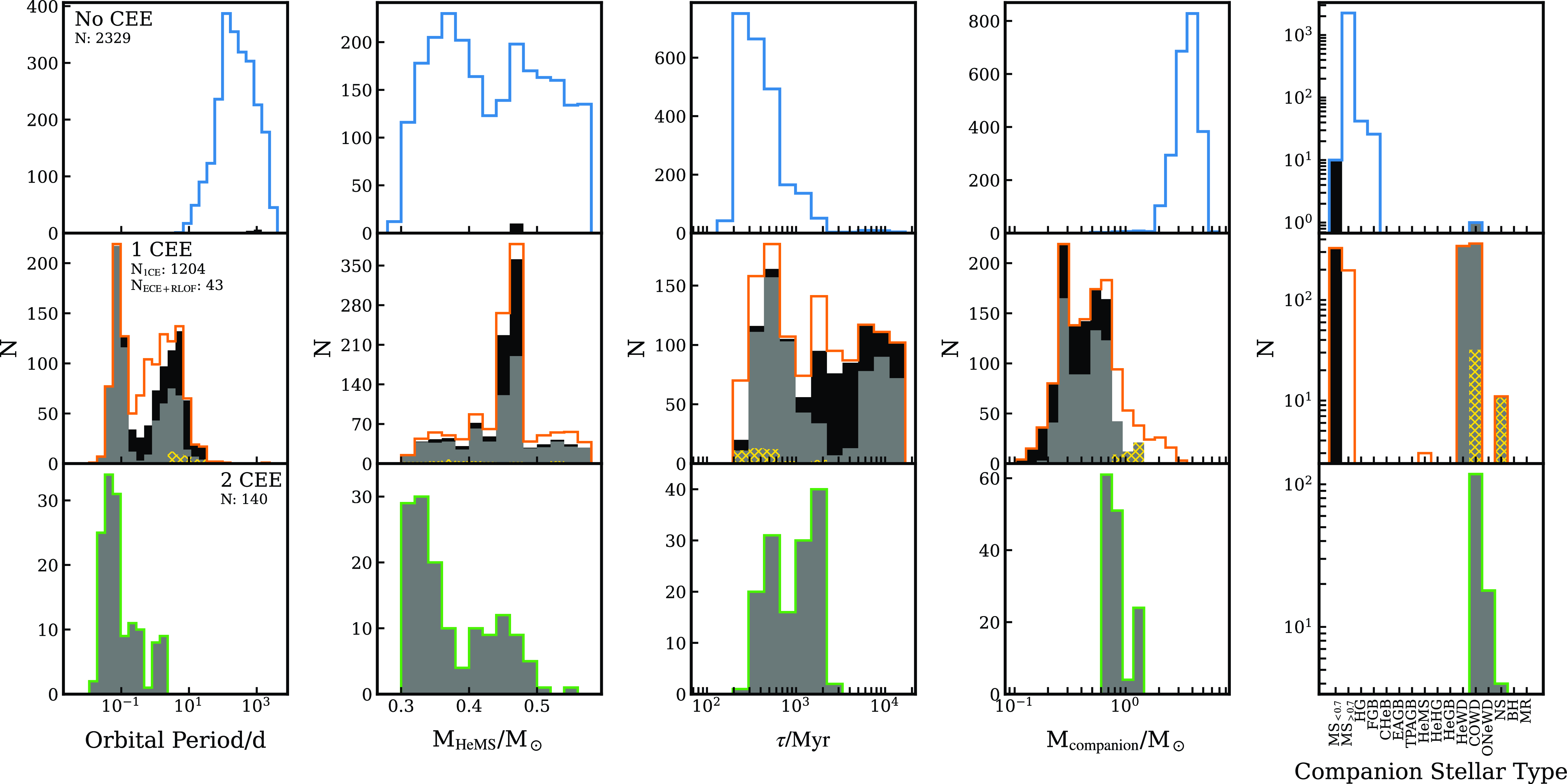
3.2. Formation channels
Considering the analysis in Section 3.1, we can see that all the studied parameters impact the final yields of our population and therefore a more in-depth analysis of sdB formation channels should only be performed after selecting a specific configuration. For this section, we chose a model based on what we consider a neutral configuration: solar metallicity, $\alpha_\textrm{CE} = 1$
, mass being lost from the position of the accretor during mass transfer, semi-efficient mass retention (
$\alpha_\textrm{CE} = 1$
, mass being lost from the position of the accretor during mass transfer, semi-efficient mass retention ( $\beta = 0.5$
), and critical mass ratios computed through the GE20 prescription. Additionally, we consider the hydrogen-rich shell prescription a necessary component, as it impacts the number of HeMS stars crossing our sdB candidate selection area in the Kiel diagram.
$\beta = 0.5$
), and critical mass ratios computed through the GE20 prescription. Additionally, we consider the hydrogen-rich shell prescription a necessary component, as it impacts the number of HeMS stars crossing our sdB candidate selection area in the Kiel diagram.
With this configuration, we find sdB formation channels similar to those described in the literature (e.g. H02): different combinations of episodes of stable mass transfer and CE episodes. Some relevant properties of these channels are shown in Fig. 13, which we analyse within the following subsections.
3.2.1. Stable mass transfer only
In this case, all our systems containing sdB candidates correspond to rather long period systems, between 10 to 3 000 days. The logarithmic period distribution peaks at about 120 days, and is slightly skewed towards longer periods. Most progenitors (about 70%) belong to the HG stage, followed by those on the FGB. Our results show that progenitors with ZAMS masses above the MHeF value are more likely to evolve into an sdB from an HG progenitor, in this case.
When it comes to the mass distribution of the sdB candidates, it is possible to distinguish two clear peaks. The first one is centered at around 0.37 M $_\odot$
, while the second one is located at 0.47 M
$_\odot$
, while the second one is located at 0.47 M $_\odot$
. The low mass peak is closely related to the aforementioned HG progenitors, while the second peak is close to the canonical mass. Finally, we note that most of these systems are formed within the initial
$_\odot$
. The low mass peak is closely related to the aforementioned HG progenitors, while the second peak is close to the canonical mass. Finally, we note that most of these systems are formed within the initial $\sim$
1 Gyr of their lifetime (
$\sim$
1 Gyr of their lifetime ( $\tau$
column in Fig. 13), with a peak at
$\tau$
column in Fig. 13), with a peak at $\sim$
250 Myr in logarithmic space, which implies that they should be more abundant in young components of the Galaxy. However, their real relevance within the current day population can only be estimated by studying the star formation history of the Galaxy.
$\sim$
250 Myr in logarithmic space, which implies that they should be more abundant in young components of the Galaxy. However, their real relevance within the current day population can only be estimated by studying the star formation history of the Galaxy.
3.2.2. One common envelope episode
For this channel, we find two different possible sub-channels: sdB candidate formation right after the CE (1CE), or formation after stable mass transfer in systems that also experienced an early CE episode (ECE+RLOF). Since the interaction that led to the formation of the sdB candidate is different, the orbital properties of such systems are different as well. This can be seen in the corresponding panels of Fig. 13, where the ECE+RLOF channel is shown as a yellow hatched area, a subset of all the systems that experienced a single CE episode pre-sdB candidate formation. This subset is restricted to periods longer than about 2 days and, although it represents only a small fraction of the total number of systems, its relevance comes from the fact that most of the sdB+NS systems follow this formation channel. For reference, the time difference between a CE episode happening first and then a stable mass transfer being triggered in sub-channel ECE+RLOF is usually a few hundreds of mega years. Though the specific characteristics and relevance of this sub-channel depend on parameters such as the chosen value for accretion efficiency (Table 1), it consistently appears throughout our populations.
Candidates formed through sub-channel 1CE peak at about 0.47 M $_\odot$
in the mass distribution, as most of the candidates within this peak come from sources initially classified as HeWDs, but considered as sdB candidates due to how close they are (5%) to the expected core mass at the tip of the RGB. The situation is different for candidates from sub-channel ECE+RLOF, as the they peak at about 0.37 M
$_\odot$
in the mass distribution, as most of the candidates within this peak come from sources initially classified as HeWDs, but considered as sdB candidates due to how close they are (5%) to the expected core mass at the tip of the RGB. The situation is different for candidates from sub-channel ECE+RLOF, as the they peak at about 0.37 M $_\odot$
, with a few candidates below the peak and the rest covering the whole range up to
$_\odot$
, with a few candidates below the peak and the rest covering the whole range up to $\sim$
0.58 M
$\sim$
0.58 M $_\odot$
.
$_\odot$
.
As previously mentioned, an important fraction of the companions from sub-channel ECE+RLOF are NS, with the remaining companions belonging to the COWD class. In the case of 1CE sub-channel, companions are predominantly MS stars and WDs.
When looking at the $\tau$
distribution, sub-channel 1CE can generally produce sdB-candidates at almost any given age after
$\tau$
distribution, sub-channel 1CE can generally produce sdB-candidates at almost any given age after $\sim$
200 Myr, though there are three spikes of sdB formation: one at the initial bin (
$\sim$
200 Myr, though there are three spikes of sdB formation: one at the initial bin ( $\sim$
200 Myr), another one around 1 800 Myr (the most prominent peak), and one above 6 000 Myr. On the other hand, the birth of sdBs from sub-channel ECE+RLOF is mostly concentrated between 200–600 Myr, peaking at about 400 Myr.
$\sim$
200 Myr), another one around 1 800 Myr (the most prominent peak), and one above 6 000 Myr. On the other hand, the birth of sdBs from sub-channel ECE+RLOF is mostly concentrated between 200–600 Myr, peaking at about 400 Myr.
3.2.3. Two common envelope episodes
This channel occurs when the initially primary star overflows its Roche lobe at an earlier time than the sdB candidate formation. This initial event leads to the removal of the primary star’s outer layers, triggering a first episode of unstable mass transfer (CE). Its outcome, however, is not the birth of the sdB candidate. Only when the initially secondary star fills its Roche lobe and the system undergoes a new CE episode, this time leading to the birth of an sdB candidate, we consider it as a member of this formation channel. In our chosen model, we get a total of 140 candidates from this channel, compared to 2 329 from the stable mass transfer channel and 1 247 in which only one CE episode is found in the system’s evolution (pre-HeMS). That means that this channel accounts for $\sim$
4% of the sdB candidates within our chosen model (without considering potential mergers), showing that it is much less common than the other two when analyzing the total numbers. Notably, these systems are mostly formed in the 300–2 000 Myr age range and peak at about 1 800 Myr.
$\sim$
4% of the sdB candidates within our chosen model (without considering potential mergers), showing that it is much less common than the other two when analyzing the total numbers. Notably, these systems are mostly formed in the 300–2 000 Myr age range and peak at about 1 800 Myr.
A clear preference for low mass HeMS stars can be seen in Fig. 13, with a peak around 0.33 M $_\odot$
and a sharp decline after the peak. A second peak seems to be present at
$_\odot$
and a sharp decline after the peak. A second peak seems to be present at $\sim$
0.45 M
$\sim$
0.45 M $_\odot$
, though it might be cause by the low number of members of this channel. The progenitors of these candidates are all FGB stars with ZAMS masses higher than 1.5 M
$_\odot$
, though it might be cause by the low number of members of this channel. The progenitors of these candidates are all FGB stars with ZAMS masses higher than 1.5 M $_\odot$
that peak around 2.3 M
$_\odot$
that peak around 2.3 M $_\odot$
, which is slightly lower than what can be found for other channels but in line with the progenitor star being the initial secondary (less massive) star. The masses of the companions at sdB-candidate formation are considerably low as well, most likely owing to the first CE episode where they should have lost a fraction of their mass during the envelope removal. Indeed, the companions are mainly COWDs with masses in the range 0.5–1.5 M
$_\odot$
, which is slightly lower than what can be found for other channels but in line with the progenitor star being the initial secondary (less massive) star. The masses of the companions at sdB-candidate formation are considerably low as well, most likely owing to the first CE episode where they should have lost a fraction of their mass during the envelope removal. Indeed, the companions are mainly COWDs with masses in the range 0.5–1.5 M $_\odot$
.
$_\odot$
.
As one would expect, the 2 CE events considerably shrink the orbital separation, and thus the period distribution peaks at about 0.04 days, with the shortest (largest) period being $\sim$
0.01 (2) days.
$\sim$
0.01 (2) days.
3.2.4. Mergers
The current version of compas does not take into account evolution beyond the formation of double WD systems and, therefore, analysis made in this subsection has been done through a simplified post-processing pipeline for informative purposes only.
First, we note that while there are ${\sim}$
40 double HeWD systems in our chosen model, only 4 of these systems have merger times below 1 Gyr (based on equation 5.10 from Peters Reference Peters1964) and thus are worth considering as plausible sdB progenitors. All remaining systems would require a time longer 14 Gyr to merge, which is a striking result, considering the non-negligible percentage of sdBs formed through mergers in H03. However, in this conservative estimate, we have not considered the consequences of excluding merging and touching stars (according to the definition in compas) from our initial sample of candidates. If we analyse these removed double HeWD systems, we get the results from Fig. 14, where it can be seen that a total of 339 sdB candidates would be formed through the HeWD+HeWD merger channel.
${\sim}$
40 double HeWD systems in our chosen model, only 4 of these systems have merger times below 1 Gyr (based on equation 5.10 from Peters Reference Peters1964) and thus are worth considering as plausible sdB progenitors. All remaining systems would require a time longer 14 Gyr to merge, which is a striking result, considering the non-negligible percentage of sdBs formed through mergers in H03. However, in this conservative estimate, we have not considered the consequences of excluding merging and touching stars (according to the definition in compas) from our initial sample of candidates. If we analyse these removed double HeWD systems, we get the results from Fig. 14, where it can be seen that a total of 339 sdB candidates would be formed through the HeWD+HeWD merger channel.
Double HeWD mergers from our chosen model, selected as systems with the Merger flag triggered in compas. Only systems that merge within 13.5 Gyr have been considered. The left panel shows the expected mass (sum of the masses of the merging HeWDs), while the right panel depicts the time that system requires to merge (since birth), e.g. the merger delay time distribution.
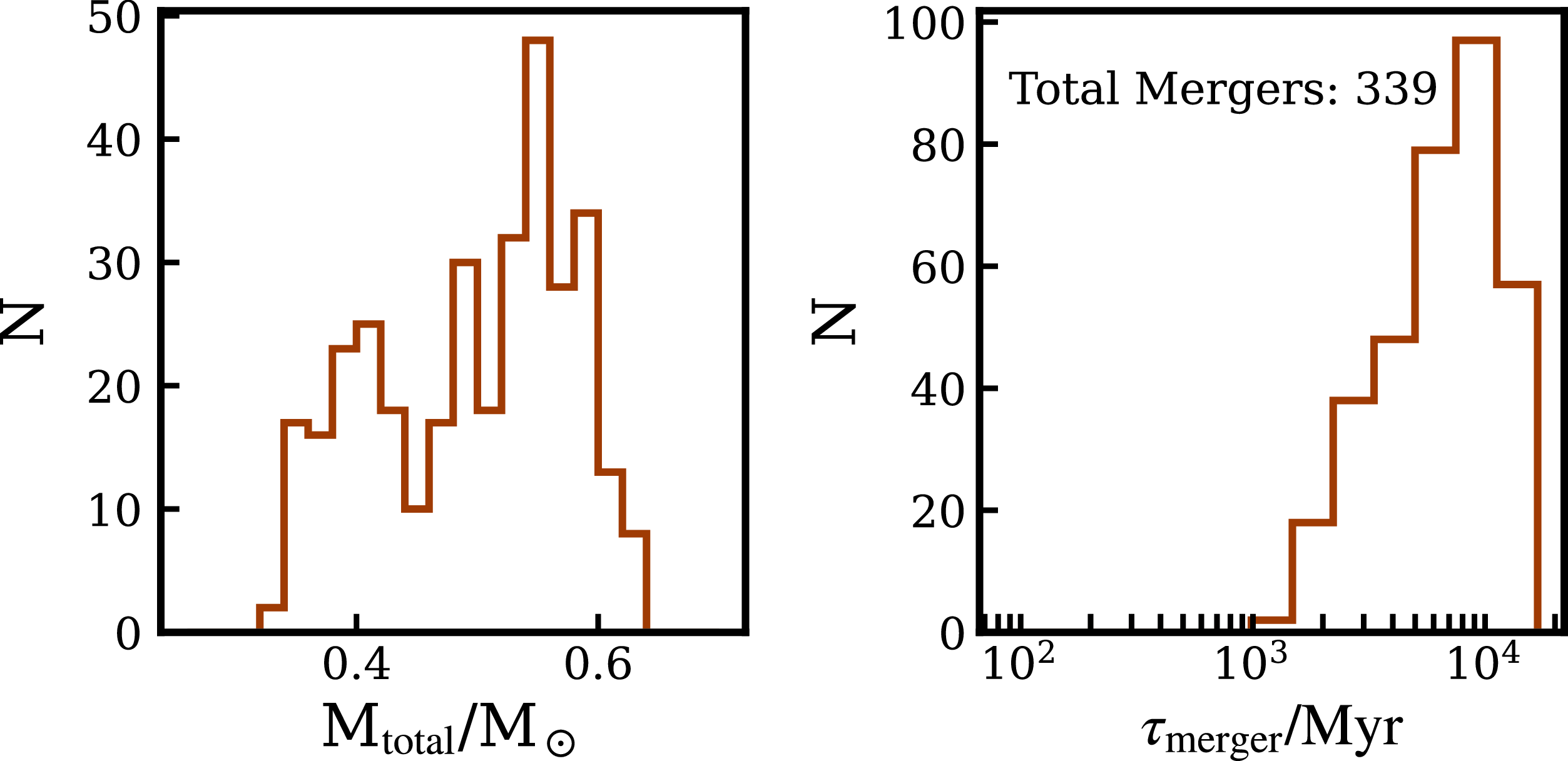
For the merger products, the mass distribution (computed as the sum of merging white dwarf masses) seems to be composed of two groups, one peaking at about 0.41 M $_\odot$
and the other at
$_\odot$
and the other at $\sim$
0.55 M
$\sim$
0.55 M $_\odot$
. For completeness purposes, we checked whether these two groups were present in cases where the accretion efficiency is 0 or 1 and found that the group peaking at low mass is strongly dependent on the choice of this value. The no-accretion case completely removes the low mass peak, while full accretion enhances it up to the point of making the distribution look symmetrical and single-peaked around
$_\odot$
. For completeness purposes, we checked whether these two groups were present in cases where the accretion efficiency is 0 or 1 and found that the group peaking at low mass is strongly dependent on the choice of this value. The no-accretion case completely removes the low mass peak, while full accretion enhances it up to the point of making the distribution look symmetrical and single-peaked around $\sim$
0.47 M
$\sim$
0.47 M $_\odot$
. However, the total time it takes a binary system from ZAMS to the merger event is strictly longer than 1 Gyr and up to 13.5 Gyr (the upper time limit we set in our simulations), with a peak at
$_\odot$
. However, the total time it takes a binary system from ZAMS to the merger event is strictly longer than 1 Gyr and up to 13.5 Gyr (the upper time limit we set in our simulations), with a peak at $\sim$
10 Gyr, no matter the accretion efficiency choice. As what was done for the systems in our chosen model, these estimates have been computed using the same Peters (Reference Peters1964) equation plus the time it takes the system to form a pair of HeWDs in compas.
$\sim$
10 Gyr, no matter the accretion efficiency choice. As what was done for the systems in our chosen model, these estimates have been computed using the same Peters (Reference Peters1964) equation plus the time it takes the system to form a pair of HeWDs in compas.
3.3. Comparison to previous studies
In line with similar work available in the literature, such as H02 and H03, we have found that channels leading to the formation of an sdB can be classified by the number and type of mass transfer events required to almost completely remove the outer hydrogen-rich layers of the progenitor. It must be noted that in Section 3.2 we only distinguish between the number of CEs and do not make the exact same analysis as the authors of H02 do, though we find general agreement between our results and the summary of sdB formation channels presented in H03.
First, we compare against their first CE ejection channel, which is roughly equal to our previously defined 1CE sub-channel: when the binary system has experienced a single CE episode that leads to the sdB candidate formation. However, for a better comparison, we select only those sdB candidates that correspond to the initially most massive (primary) star of the system, and we also include stars that were classified as HeWDs by compas (but can be considered as candidates according to Section 3.1.5, setting a 5% threshold). With these constraints in place we find general agreement with properties presented in H03: most of the progenitors are classified as FGB stars (the exception being a few CHeB stars), the masses of the candidates show a sharp peak at $\sim$
0.46 M
$\sim$
0.46 M $_\odot$
, and the companions are in the MS stage. For stars born from progenitors with masses below MHeF, we find a similar minimum period, on the order of
$_\odot$
, and the companions are in the MS stage. For stars born from progenitors with masses below MHeF, we find a similar minimum period, on the order of $10^{-1}$
days (twice the H03 value), and our maximum period is around 30 days, which is a bit different from what is reported in H03 as they mention a maximum period
$10^{-1}$
days (twice the H03 value), and our maximum period is around 30 days, which is a bit different from what is reported in H03 as they mention a maximum period $\geq$
40 days. We note that this maximum period value can be increased by, for example, changing our choice of critical mass ratio prescription from GE20 to NONE, raising our maximum period to around 50 days. Additional small discrepancies are found for candidates born from progenitors with ZAMS masses higher than MHeF, considering that they are described as products of HG stars resulting in low HeMS masses, while we find instead that our candidates are all in the FGB and cover a wide (0.3–0.6 M
$\geq$
40 days. We note that this maximum period value can be increased by, for example, changing our choice of critical mass ratio prescription from GE20 to NONE, raising our maximum period to around 50 days. Additional small discrepancies are found for candidates born from progenitors with ZAMS masses higher than MHeF, considering that they are described as products of HG stars resulting in low HeMS masses, while we find instead that our candidates are all in the FGB and cover a wide (0.3–0.6 M $_\odot$
) mass range without a well defined peak. We should remark, however, that we do find these systems with more massive progenitors restricted to short periods (
$_\odot$
) mass range without a well defined peak. We should remark, however, that we do find these systems with more massive progenitors restricted to short periods ( $\lesssim$
1 days), as pointed out by H03.
$\lesssim$
1 days), as pointed out by H03.
We then proceed to analyse the first stable RLOF channel presented by H03, described as being composed of sdB candidates with MS companions in wide orbits that cover the 0.5–2 000 days period range. There is agreement if we compare against sdB candidates formed after the initially primary star overflows its Roche lobe and loses its outer layers through stable mass transfer in our chosen model, particularly finding companions in the same evolutionary stage (MS) and a similar orbital period range. In our case, the periods cover the 5 to $\gtrsim$
3 000 day range, though it should be noted that there is a constant decrease in the number of systems for periods greater than 500 days. H03 also mention that the short period systems are stars going through the start of the HG and, although we have not verified in which section of the HG our candidates lost most of their outer hydrogen-rich layers, we find that the short period end of our period distribution (5 to
$\gtrsim$
3 000 day range, though it should be noted that there is a constant decrease in the number of systems for periods greater than 500 days. H03 also mention that the short period systems are stars going through the start of the HG and, although we have not verified in which section of the HG our candidates lost most of their outer hydrogen-rich layers, we find that the short period end of our period distribution (5 to $\sim$
500 days, peaking at about 100 days) is also composed of HG stars. For reference, candidates born from FGB stars cover the 50–3 000 days period range, while we find fewer CHeB progenitors in the 500–3 000 day period range. Going back to the HG progenitor group, H03 comment on a wide mass distribution range, which is also observed in our sample, though our upper sdB mass is restricted by our initial cut at 0.58 M
$\sim$
500 days, peaking at about 100 days) is also composed of HG stars. For reference, candidates born from FGB stars cover the 50–3 000 days period range, while we find fewer CHeB progenitors in the 500–3 000 day period range. Going back to the HG progenitor group, H03 comment on a wide mass distribution range, which is also observed in our sample, though our upper sdB mass is restricted by our initial cut at 0.58 M $_\odot$
.
$_\odot$
.
The analysis of H03’s second CE ejection channel is rather similar to the first CE ejection one, though in this case companions are in the WD stage. The characteristics of this configuration imply that its final product should be systems with periods shorter than the ones found in previous configurations, and also that the range covered by the period distribution could be wider. Due to these properties, we compare this channel to our sdB candidates born after two CE episodes, the bottom panels in Fig. 13. As can be understood from the distributions, we do find that most of the companions are COWDs, with a small contribution of ONeWDs and an even smaller fraction of NSs. A striking difference to the H03 predictions is that, although all our periods are shorter than the ones found in other channels and clustered around 0.05 days, they do not cover the expected wider range when compared to the first CE channel. In this scenario, it is possible to realise that some members of our 1CE episode channel actually match the definition of H03’s second CE ejection, in which case the period range being covered is indeed wider, going up as far as $\sim$
100 days. If this is the case, however, the period peak is slightly displaced towards longer periods at 0.1 days. Further, the peaks in mass distribution for the subset of stars that have experienced 2 CE episodes and have progenitor masses above (below) the MHeF limit match the predictions of H03, with a value of
$\sim$
100 days. If this is the case, however, the period peak is slightly displaced towards longer periods at 0.1 days. Further, the peaks in mass distribution for the subset of stars that have experienced 2 CE episodes and have progenitor masses above (below) the MHeF limit match the predictions of H03, with a value of $\sim$
0.33 (
$\sim$
0.33 ( $\sim$
0.46) M
$\sim$
0.46) M $_\odot$
. The more massive progenitors (above MHeF) account for most of the systems found, in line with the description of H03.
$_\odot$
. The more massive progenitors (above MHeF) account for most of the systems found, in line with the description of H03.
H03 also include the merger channel, which usually represents a non-negligible fraction of the total amount of the sdB candidates in all their populations (see their Tables 1 and 2). Our mergers have not been analyzed through detailed models as what has been done in H02, which means that our results are referential and would only set an upper limit to the total number of sdBs being formed through this process (i.e. some of our mergers could be stars that do not ignite helium or follow a different evolutionary path). Nevertheless, we can see agreement in the mass range of our merger candidates.
We also note that figure 5 in H02 is similar to our Fig. 12, though the observational sample currently available is much richer and the hydrogen-rich layer treatment is different. Probably because of this reason, and the fact that we have not conducted a current day population study, the coverage within the Kiel diagram more readily matches the observations in our work.
We briefly address a different study by Clausen et al. (Reference Clausen, Wade, Kopparapu and O’Shaughnessy2012), who mention the relevance of hydrogen-rich shell in sdBs, but do not implement them within their rapid BPS code. Instead, they check whether their sdB candidates would remain in the $\log{g}$
-
$\log{g}$
- $\log{T}$
box (chosen as their definition of sdBs) if those same stars had hydrogen-rich shells, based on results of Caloi (Reference Caloi1972). However, their lower limit for surface gravity is set at
$\log{T}$
box (chosen as their definition of sdBs) if those same stars had hydrogen-rich shells, based on results of Caloi (Reference Caloi1972). However, their lower limit for surface gravity is set at $\log{g} = 5$
, leaving a non-negligible fraction of the observational sample out of their parameter study (see Fig. 12).
$\log{g} = 5$
, leaving a non-negligible fraction of the observational sample out of their parameter study (see Fig. 12).
Another important element raised by Clausen et al. (Reference Clausen, Wade, Kopparapu and O’Shaughnessy2012) is the mass cutoff for helium ignition. They consider both a 0 and 5% cutoff value through their $f_{He}$
parameter, similar to what we have explored in our parameter variations. Accordingly, the impact in their population is evident, as can be concluded from comparing any pair of runs where only the
$f_{He}$
parameter, similar to what we have explored in our parameter variations. Accordingly, the impact in their population is evident, as can be concluded from comparing any pair of runs where only the $f_{He}$
is different in their table 1. For example their run 6 has about 15 times more resampled systems than run 7, which is potentially related to the spike that appears when considering a non-zero threshold in Fig. 7.
$f_{He}$
is different in their table 1. For example their run 6 has about 15 times more resampled systems than run 7, which is potentially related to the spike that appears when considering a non-zero threshold in Fig. 7.
We note, however, that a direct one-to-one comparison is not possible at this point, particularly because our study does not predict a current-day population and therefore many of the conclusions drawn within Clausen et al. (Reference Clausen, Wade, Kopparapu and O’Shaughnessy2012) cannot be tested. We intend to present our estimates of the current-day sdB population in a following study.
4. Conclusions
We have explored parameters influencing the different sdB formation channels and their characteristics as predicted by compas. Our results are in agreement with previous studies that have used population synthesis to analyze the properties of these stars, showing that compas and the prescription for hydrogen-shells are elements that further expand the set of tools available when analyzing sdBs. A more in-depth comparison with previous studies and the current day Galactic population of sdBs requires additional work, including a sampling based on the Galactic star formation rate and the different mass fractions and metallicities of each component of the Galaxy (Bulge, Disks, and Halo), elements which we intend to analyze in a future publication. We foresee that this upcoming study will allow a comparison between our 1CE channel and, e.g. Schaffenroth et al. (Reference Schaffenroth, Pelisoli, Barlow, Geier and Kupfer2022), potentially providing an additional constraint to the parameters explored in the current work. Similarly, it will be possible to compare the total number of sdBs in the Galaxy at the current epoch as predicted by the compas BPS approach against the observational results of the 500pc sample (Dawson et al. Reference Dawson2024).
Moreover, the improved coverage of the sdB box within the Kiel diagram highlights the potential of our prescription for sdBs with hydrogen-rich shells to further improve the predictions of rapid BPS models, particularly when it comes to comparing to observables linked to stellar radii and luminosity, such as the surface gravity and effective temperature distributions. An extended coverage of the models towards more massive sdBs would be ideal to further improve our predictions and avoid unnecessary mass cuts in the population, while a detailed study on the hydrogen-rich envelope relation with the different formation channels could impose additional constraints on the population. If each sub-channel presents a different hydrogen-envelope mass distribution, unlike the randomly sampled envelopes of our work, then we could check whether the corresponding number and characteristics of the sdBs born through each channel are in agreement with the observed Galactic sdB population or not. These potential differences could stem from the characteristics (stability) of the mass transfer episode that gives birth to a given sdB population.
We also note that it is still complicated to disentangle the different factors contributing to the observed characteristics of each analyzed physical property, in cases such as the period and mass distributions of the different formation channels. Moreover, additional parameters not explored in this work could reveal yet more properties and/or constraints for the evolution of sdBs, such as the case of magnetic braking (e.g. Blomberg, El-Badry, & Breivik Reference Blomberg, El-Badry and Breivik2024) and companions below the hydrogen burning limit (Brown Dwarfs, see e.g. Schaffenroth et al. Reference Schaffenroth, Pelisoli, Barlow, Geier and Kupfer2022). We highlight, however, that the companion mass distribution could potentially constrain the angular momentum loss and critical mass prescriptions. Similarly, the mass distribution of sdBs with periods in the range $\sim$
1–10 days could help to further test the threshold at which naked cores with masses below the expected helium-core mass at helium ignition would indeed ignite and become sdBs.
$\sim$
1–10 days could help to further test the threshold at which naked cores with masses below the expected helium-core mass at helium ignition would indeed ignite and become sdBs.
Finally, our chosen model (not to be confused with a best model, since we have not compared with the current-day Galactic sdB population) predicts the existence of sdB plus NS systems being born through a very specific channel, which we labeled as ECE+RLOF. While the expected occurrence of these systems seems to be low, it is interesting that a big fraction of them are born from systems that experience an early CE (ECE) episode, but the sdB candidate is born from a late stable mass transfer event. Even though we also predict sdB + NS systems from the 2CE channel, the ECE+RLOF one should be $\sim$
10 times more common, with periods longer than 1 day. Another interesting type of systems that can be found in our results are COWD+sdB pairs from the 1CE or 2CE channel, which can be understood as potential gravitational wave sources (owing to their close orbits) and will be of interest for LISA. The formation rate of these events is also something that we expect to predict in a future publication where a Galaxy-like population will be studied.
$\sim$
10 times more common, with periods longer than 1 day. Another interesting type of systems that can be found in our results are COWD+sdB pairs from the 1CE or 2CE channel, which can be understood as potential gravitational wave sources (owing to their close orbits) and will be of interest for LISA. The formation rate of these events is also something that we expect to predict in a future publication where a Galaxy-like population will be studied.
Acknowledgements
We thank the anonymous referee for their helpful comments. NRS thanks Evan Bauer for insightful discussions, and also acknowledges valuable support received from the compas team, particularly from Reinhold Willcox, Ilya Mandel, Jeff Riley and Alejandro Vigna-Gómez. AJR acknowledges financial support from the Australian Research Council under award number FT170100243.
Data availability statement
All data will be available upon reasonable request to the corresponding author.
Appendix A. Complete List of Configurations
The specific configuration for each run is shown in Table A1. Even though there are some degeneracies due to no angular momentum loss at full accretion, we have kept all sets in order to compare similar numbers of candidates during each parameter variation.
Parameters used on each compas configuration set. Proprieties not listed here were kept as default, or already specified in Table 1.
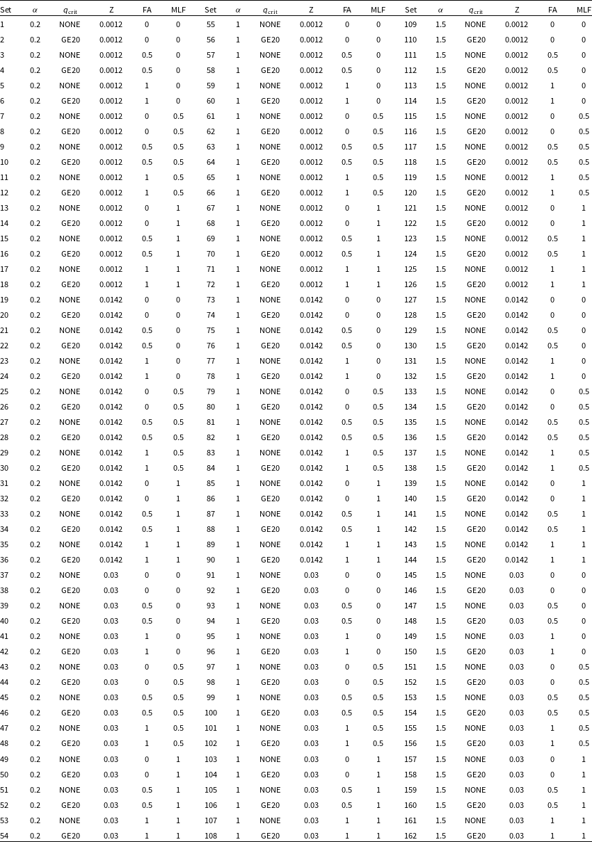
Appendix B. Coefficients for Fits
B.1. Lifetime
The lifetime (maximum age) of a HeMS star with a hydrogen-rich shell can be computed by using Equation 15, and the different $A_i$
coefficients are shown in Table B1.
$A_i$
coefficients are shown in Table B1.
Coefficients for age fit, as presented in Equation (15).
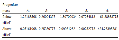
B.2. Radius
The coefficients of the fit shown in Equation (17) can be computed using one of the following forms:
 \begin{align} F_1 = \left(a + bM + cM^2\right)\left(d + eM_\textrm{H} + fM^2\right) + g + hM_\textrm{H}, \end{align}
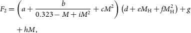 \begin{align} F_2 &= \left(a + \frac{b}{0.323 - M + iM^2} + cM^2\right)\left(d + eM_\textrm{H} + fM_\textrm{H}^2\right) + g \nonumber\\[5pt] &\quad + hM, \end{align}
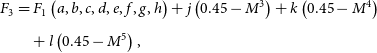 \begin{align} F_3 &= F_1\left(a,b,c,d,e,f,g,h\right) + j\left(0.45 - M^3\right) + k\left(0.45 - M^4\right)\nonumber \\[5pt] & \quad + l\left(0.45 - M^5\right),\end{align}
while the specific details of the $a,b,...,k,l$
constants for each
$a,b,...,k,l$
constants for each $B_i$
coefficient are given in Table B2.
$B_i$
coefficient are given in Table B2.
Coefficients used in the radius fit, as presented in Equation (17). The specific form of each $F_i$
expression is defined in Appendix B.2.
$F_i$
expression is defined in Appendix B.2.
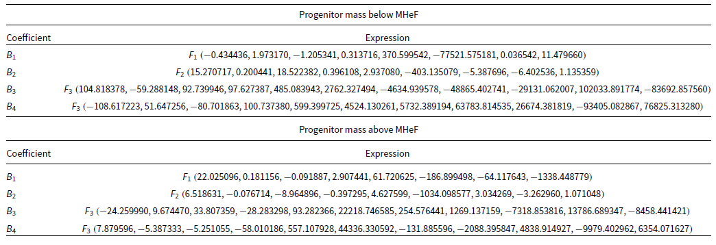
B.3. Luminosity
Similar to what was done for the stellar radius, the coefficients of the fit applied to luminosity and shown in Equation (18) require one of the following:
 \begin{align} F_4 = \left(a + bM + cM^2\right)\left(d+eM_\textrm{H}\right) + f + gM_\textrm{H}, \end{align}
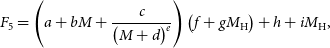 \begin{align} F_5 = \left(a +bM + \frac{c}{\left(M + d\right)^{e}}\right)\left(f + gM_\textrm{H}\right) + h + iM_\textrm{H}, \end{align}
 \begin{align} F_6 = \left(a + bM + cM^2 + dM^5\right)\left(e + fM_\textrm{H}\right) + g + hM_\textrm{H},\end{align}
with specific values corresponding to the $a,b,...,h,i$
constants required for each
$a,b,...,h,i$
constants required for each $C_i$
being shown in Table B3.
$C_i$
being shown in Table B3.
Graphic comparison between the prescription developed in Section 2.2.1 (red lines) and the models from Bauer & Kupfer (Reference Bauer and Kupfer2021) (solid grey lines). On the top-left corner of the left-hand side panels, information related to the properties of the HeMS model in each row is given in the format mass at ZAMS (M $_\odot$
), HeMS mass (M
$_\odot$
), HeMS mass (M $_\odot$
), metallicity (Z). A similar annotation in the middle panel shows the total time spent (Myr) in the HeMS stage.
$_\odot$
), metallicity (Z). A similar annotation in the middle panel shows the total time spent (Myr) in the HeMS stage.
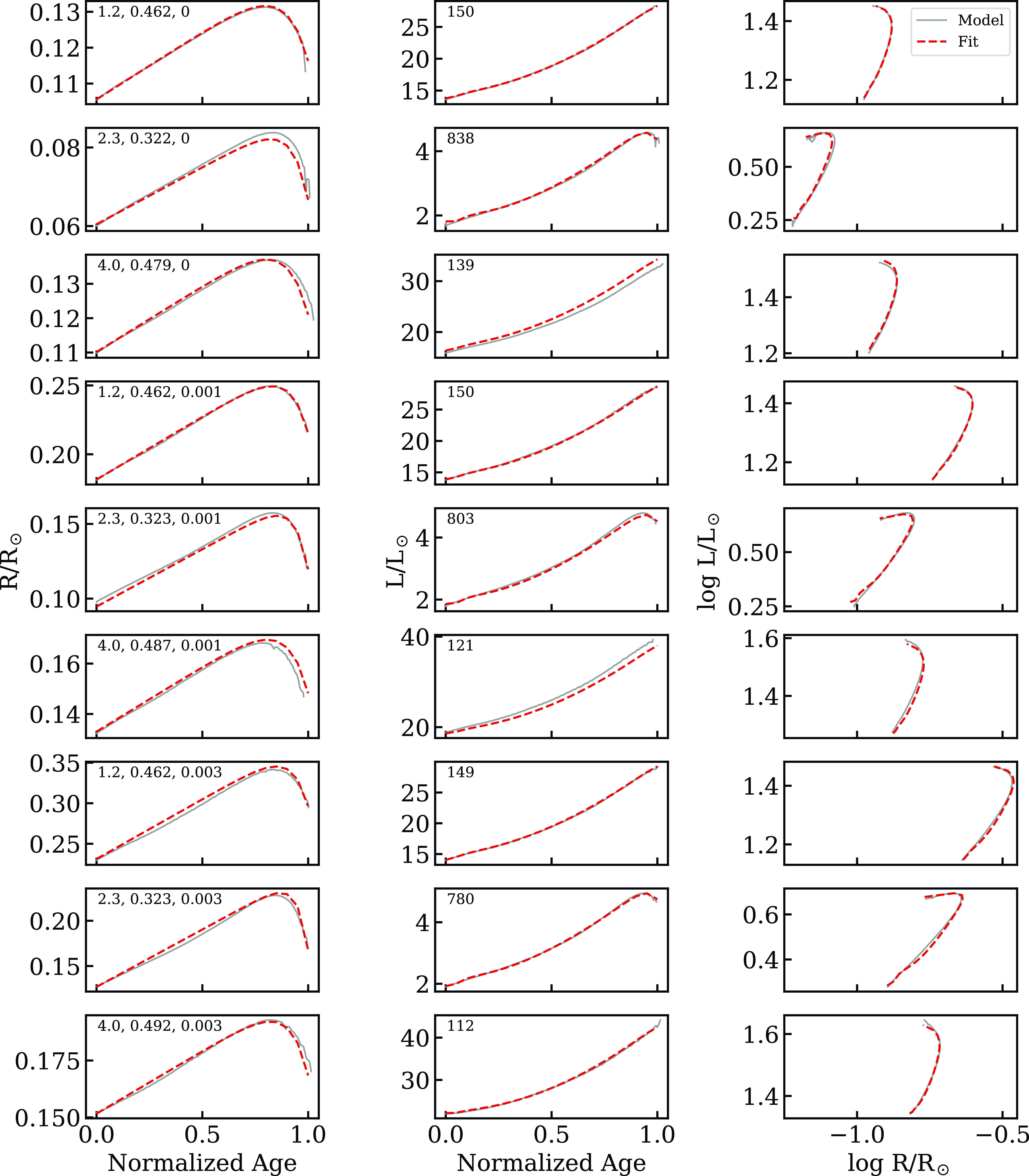
Coefficients for the luminosity fit, as presented in Equation 18. The relevant $F_i$
expressions are defined in appendix B.3.
$F_i$
expressions are defined in appendix B.3.
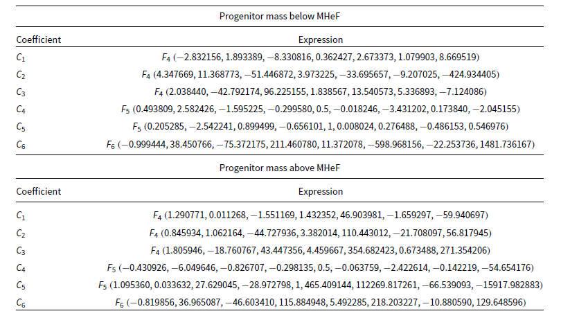


 Open access