

1. Introduction
Glaciers on the Tibetan Plateau have undergone significant changes since the latter half of the last century (Hugonnet and others, Reference Hugonnet2021). Glacier length retreat is one of the most prominent indicators of glacier change (Bolch and others, Reference Bolch2012). The ongoing retreat of glaciers alters the relative contribution of ice melt, snow melt and groundwater to proglacial mountain-river systems (Wang and others, Reference Wang2024a, Reference Wang2024b), thereby affecting downstream freshwater supply (Brown and others, Reference Brown, Hannah and Milner2007). Projections under future climate scenarios suggest that by 2050, glacier mass loss across the Tibetan Plateau may lead to a reduction in river discharge by 8.4% for the Indus, 17.6% for the Ganges, 19.6% for the Yarlung Tsangpo–Brahmaputra and 5.2% for the Yangtze River, posing serious risks to agriculture, hydropower generation and water security in densely populated downstream regions (Immerzeel and others, Reference Immerzeel, Beek and Bierkens2010; Yao and others, Reference Yao, Wu, Xu, Wang, Gao and An2019). In addition, glacier retreat disrupts local ecosystems and biodiversity by altering land cover around the glacier termini and threatening multiple rare species (Jacobsen and others, Reference Jacobsen, Milner, Brown and Dangles2012; Giersch and others, Reference Giersch, Hotaling, Kovach, Jones and Muhlfeld2016; Fell and others, Reference Fell, Carrivick and Brown2017).
Variations in climate change and glacier response properties are primary factors leading to inhomogeneous glacier changes across different regions (Bhattacharya and others, Reference Bhattacharya2021). Many studies have indicated that local physiographic factors, apart from climate change, also drive the heterogeneous pattern of glacier retreat. Proglacial lakes are lakes that are in direct contact with glacier termini. The formation and rapid expansion of such lakes have shown to significantly accelerate mass loss of their host glaciers (King and others, Reference King, Bhattacharya, Bhambri and Bolch2019; Sutherland and others, Reference Sutherland, Carrivick, Gandy, Shulmeister, Quincey and Cornford2020). This enhanced mass loss is primarily associated with intensified frontal ablation at the interface between the glacier and the lake, where mechanical calving represents the dominant process (Robertson and othersReference Robertson, Benn, Brook, Fuller and Holt2012; Truffer and Motyka, Reference Truffer and Motyka2016; Minowa and others, Reference Minowa, Sugiyama, Sakakibara and Skvarca2017; Watson and others, Reference Watson, Kargel, Shugar, Haritashya, Schiassi and Furfaro2020; Dye and others, Reference Dye, Bryant and Rippin2022).
The importance of calving for glacier mass loss has been widely documented. For instance, Motyka and others (Reference Motyka, Hunter, Echelmeyer and Connor2003) reported that calving accounted for 57% of the mass loss at LeConte glacier in Alaska, and Greene and others (Reference Greene, Gardner, Wood and Cuzzone2024) found that excluding calving can underestimate Greenland Ice Sheet mass loss by up to 20% from 1985 to 2022. Glacial calving can accelerate glacial retreat if the calving velocity surpasses the ice flux near the terminus. For example, lake-terminating glaciers in southcentral Alaska retreated by 2.3–5.2 km during 1984–2021, while land-terminating glaciers experienced length changes ranging from −2.1 to 0.21 km during the same period (Black and others, Reference Black and Kurtz2023). Similar contrasts have been reported in High Mountain Asia. During 1988–2018, the lake-terminating Glacier Longbasaba in the central Himalaya retreated at an average rate of 51.7 m a−1, far exceeding that of the adjacent land-terminating glacier (7.8 m a−1) (Liu and others, Reference Liu2020). More recently, the lake-terminating Duiya glacier in the middle Himalayas retreated by 220 m from 2017 to 2021 (Shi and others, Reference Shi2024).
The Jiongpu Co Lake (30°39′44″ N, 94°29′01″ E), one of the largest proglacial lakes on the South-eastern Tibetan Plateau, is mainly fed by a single large glacier (Fig. 1). The area of the Jiongpu Co Lake expanded from 0.6 km2 in 1967 to 5.68 km2 in 2020, due to the rapid shrinkage of its host glacier providing space and meltwater (Zhao and others, Reference Zhao, Cheng, Guan, Zhang and Cao2024). According to meteorological station records, the annual air temperature and precipitation in this Basin are approximately 8.5°C and 1000 mm, respectively (Ke and others, Reference Ke, Lee and Han2019). A previous study demonstrated that neglecting subaqueous mass loss led to a 21% underestimation of the total mass loss for this glacier during 2000–2020 (Li and others, Reference Li2024). Zhao and others (Reference Zhao, Cheng, Guan, Zhang and Cao2024) further revealed that the proportion of frontal ablation in total mass loss increased from 26% (1985–2000) to 52% (2010–2020), coinciding with accelerated expansion of the proglacial lake. Simultaneously, the continuous enlargement of this proglacial lake triggered rapid mass loss from its host glacier, resulting in a retreat of approximately 800 m at the glacier terminus between 17 October 2014 and 30 November 2015. This event represented the fastest reported glacial retreat on the Tibetan Plateau.

Figure 1. Jiongpu Co Glacier and the proglacial lake location. (a) White and blue borders represent the glacier and glacial lake boundaries as of 15 November 2015, respectively, while the red line indicates the position of glacier–glacial lake contact on 17 October 2014. The orange line is the position of the flux gate defined in this study. The 0–8 km markers show the cross-section from the lake outlet extending 8 km upstream. (b) Jiongpu Co Glacier and proglacial lake location in the Tibetan Plateau. The SRTM V1 DEM was used in the figure.
In this study, we reconstruct the detailed glacier–lake evolution during this period using multi-source remote sensing imagery. We analyze the calving activity and potential causes of the rapid terminus retreat and quantify the associated mass loss. This work provides a rare event-scale perspective on glacier instability and enhances our understanding of lake-terminating glacier dynamics in High Mountain Asia.
2. Materials and methods
2.1. Datasets
Eleven Landsat Operational Land Imager (OLI) Level1 (L1) and two Chinese Gaofen-1 (GF-1) multispectral images were used to extract the outlines of the Jiongpu Co Glacier between 17 October 2014 and 30 November 2015 (Paul and others, Reference Paul2015; Yan and Wang, Reference Yan and Wang2019) (Table S1). The Landsat data, with a spatial resolution of 30 m and downloaded from the United States Geological Survey, were processed through radiometric calibration, atmospheric correction, geometric correction and terrain correction. The GF-1 wide field view (WFV) L1 multispectral images, with a spatial resolution of 16 m, were obtained from the China Centre for Resources Satellite Data and Application (CASC).
Twenty single-look complex synthetic aperture radar (SAR) images from Sentinel-1 were used to analyze detailed surface velocity patterns of Jiongpu Co Glacier (Table S1). Sentinel-1 is an Earth Radar Observatory satellite jointly operated by the European Commission and the European Space Agency under the Copernicus program (Malenovský and others, Reference Malenovský2012). Compared to optical satellites, microwave radar satellites have a major advantage of operating independently of solar illumination and being able to penetrate clouds. The satellite operates around the clock, using a C-band SAR for imaging purposes and follows a 12 d repeated cycle in orbit. Previous studies have demonstrated that Sentinel-1 SAR images in interferometric wide swath mode, with a range resolution of 5 m and an azimuthal resolution of 20 m, are suitable for extracting glacier velocity (Nagler and others, Reference Nagler, Rott, Hetzenecker, Wuite and Potin2015; Lemos and others, Reference Lemos, Shepherd, McMillan, Hogg, Hatton and Joughin2018; Friedl and others, Reference Friedl, Seehaus and Braun2021).
The depth of Jiongpu Co Lake was measured using an uncrewed autonomous vessel equipped with a single-beam sonar system in 2020 and 2021. The sonar operated at 200 kHz frequency and collected depth measurements at uniform time intervals. Bathymetric results indicated that the maximum depth of the lake was 245 m, which was calculated by the universal kriging spatial interpolation of 2658 evenly distributed sample points, with an average depth of 124 m (Fig. 2). Measurement uncertainty, evaluated through comparison with rope measurements at seven validation points, was less than 4% (Fig. S2) (Li and others, Reference Li2024).

Figure 2. Bathymetry of Jiongpu Co Lake, with 40 m interval contour lines. The insert shows the lake bed morphology along profile AA′ (approximately 6 km from outlet of lake to glacier terminus in 2020) and the positions of the glacier terminus and lake depth for specific years. The glacier terminus positions in the main map are color-coded using the same scheme as in the insert visual consistency. The base map in this figure is sourced from online maps published by the plugin MapOnlineV1.2 in ArcMap.
2.2. Methods
2.2.1. Changes in glacier length
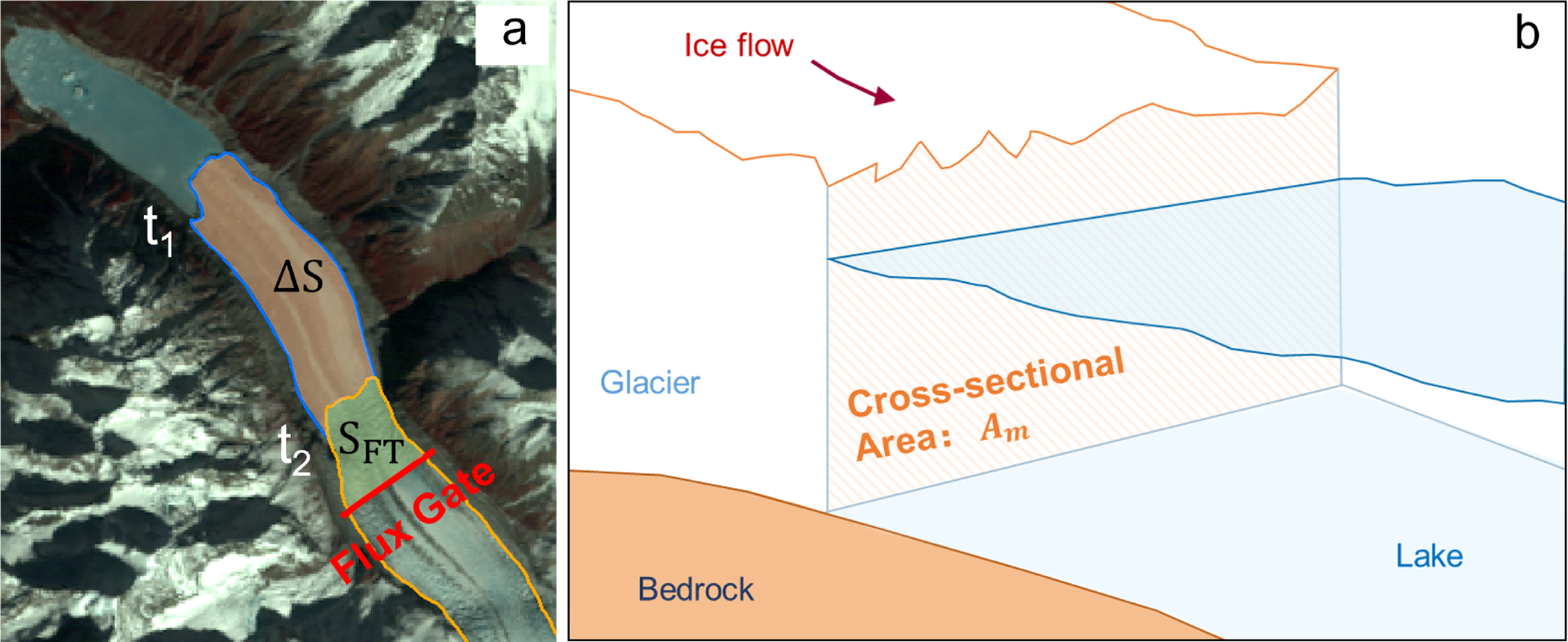
The panchromatic band of the Landsat image was fused with the multispectral bands (red, green and blue mapped to NIR, red and green bands, respectively) using a pan-sharpening technique to enhance the spatial resolution of the composite image to 15 m. For GF-1 WFV L1 multispectral images, radiometric calibration, FLAASH atmospheric correction and orthorectification were performed in ENVI software. The glacier outlines between 17 October 2014 and 30 November 2015 were manually mapped based on Landsat OLI and GF-1 images. Change in glacier length was calculated by dividing glacier area change below the flux gate by width of the flux gate, where the flux gate is defined as a transverse cross section across the glacier oriented approximately perpendicular to the ice flow direction (Moon and Joughin, Reference Moon and Joughin2008). In this study, the flux gate was positioned approximately 7.2 km upstream from the Jiongpu Co Lake outlet and oriented as perpendicular as possible to the ice flow direction (Fig. 1).
2.2.2. Glacier surface velocity
Offset-tracking of SAR imagery has recently been widely used to extract glacier surface displacements with a theoretical accuracy reaching 1/10 of a pixel (Heid and Kääb, Reference Heid and Kääb2012; Paul and others, Reference Paul2015, Reference Paul2017). We utilized the offset-tracking algorithm in the GAMMA software (Wegmüller and Werner, Reference Wegmüller and Werner1997) to extract surface velocity of the Jiongpu Co Glacier at 24 d intervals between 22 October 2014 and 16 December 2015 through Sentinel-1 SAR images.
In this study, we applied a correlation threshold (coherence value <0.2) to the offset tracking results to exclude poorly correlated displacement values (Nakamura and others, Reference Nakamura, Doi and Shibuya2007). We then filtered the results by comparing horizontal displacement direction with the surface aspect, removing velocity values where the angular difference exceeded 60° to eliminate anomalous flow directions errors (Ruiz and others, Reference Ruiz, Berthier, Masiokas, Pitte and Villalba2015). Finally, we statistically removed displacements falling outside of (μ − 3σ, μ + 3σ) (where μ represents the mean value and σ is standard deviation) in the Gaussian distribution for each result, in order to exclude unrealistic velocity values caused by avalanches, rockfalls and other factors (Scherler and others, Reference Scherler, Leprince and Strecker2008; Ruiz and others, Reference Ruiz, Berthier, Masiokas, Pitte and Villalba2015).
Previous studies have indicated that the accuracy of the glacier surface velocities can be evaluated by examining surface displacement in relatively stable regions (Guan and others, Reference Guan2022; Paul and others, Reference Paul2017). Thus, we evaluated the precision of the velocities obtained using the offset-tracking algorithm by calculating surface displacement in non-glaciated areas with slopes lower than 10° within the region. The results showed uncertainty of surface velocities extracted from Sentinel-1 SAR images ranging from 0.02 to 0.07 m d−1 (Fig. S1).
2.2.3. Glacier mass loss
For lake-terminating glaciers, total mass loss is primarily composed of frontal ablation due to calving and subaqueous melt, in addition to surface mass loss (King and others, 2019). Frontal ablation ( ${A_{\text{f}}}$) can be further split into two components: ice discharge (
 ${D_{{\text{ice}}}}$) across a flux gate and the mass change associated with glacier terminus position change (
 ${M_{{\text{term}}}}$) (Kochtitzky and others, Reference Kochtitzky2022). Accordingly, the total mass loss of lake-terminating glaciers (
 ${M_{\text{t}}}$) can be expressed by:
 \begin{equation}M_\text{t}=A_\text{f}+M_\text{s}=\left(D_\text{ice}+M_\text{term}\right)+M_\text{s}\end{equation}
 Here,  ${M_{\text{s}}}$ represents surface mass loss.
 ${D_{{\text{ice}}}}$ is given by:
 \begin{equation}D_\text{ice}=\rho_\text{ice}\cdot\overline v\cdot t\cdot{\overline h}_\text{F}\cdot D+S_\text{FT}\cdot{\overline b}_\text{clim}\cdot t\end{equation}
where  ${\rho _{{\text{ice}}}}$ is the vertically averaged ice column density with a value of 900 kg m−3 (Kääb and others, Reference Kääb, Berthier, Nuth, Gardelle and Arnaud2012);
  $\bar v$ is average velocity at the glacier flux gate (m d−1);
  $t$ represents the interval time (d);
  ${\bar h_{\text{F}}}$ represents the mean ice thickness along the flux gate at time
  ${t_1}$ (m);
  $D$ is the width of the glacier flux gate;
  ${S_{{\text{FT}}}}$ is the area of the region between the glacier terminus front at time
  ${t_2}$ and the flux gate (Fig. 3a) (m2);
  ${\bar b_{{\text{clim}}}}$ represents the average climatic mass balance for region
  ${S_{{\text{FT}}}}$ (kg m−2 d−1; accumulation positive, ablation negative).

Figure 3. (a) Map shows the regions  $\Delta S$ and
  ${S_{{\text{FT}}}}$, where
  $\Delta S$ represents the change in glacier area between observation times
  ${t_1}$ and
  ${t_2}$, and
  ${S_{{\text{FT}}}}$ denotes the glacier area below the flux gate used to calculate glacier mass loss. The base map in this figure is from Landsat 8 OLI images. (b) Diagram shows the cross-sectional area
  ${A_{\text{m}}}$ at the glacier terminus at times
  ${t_2}$, which is used for the calculation of calving velocity.
 ${M_{{\text{term}}}}$ is calculated by taking the glacier mass loss within the region (
 $\Delta S$) where glacier terminus position changed between times
  ${t_1}$ and
  ${t_2}$ and subtracting the surface mass loss over that same area. The calculation formula is as follows:
 \begin{equation}{M_{{\text{term}}}} = {\rho _{{\text{ice}}}} \cdot \Delta S \cdot {\bar h_{\Delta S}} - \left( { - 0.5 \cdot \Delta S \cdot {{\bar b}_{{\text{clim}}\Delta S}} \cdot t} \right)\end{equation}
where  $\Delta S$ represents the area lost at the glacier terminus between time
  ${t_1}$ and
  ${t_2}$ (Fig. 3a) (m2);
  ${\bar h_{\Delta S}}$ represents the average ice thickness at the area
  $\Delta S$ (m);
 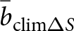 ${\bar b_{{\text{clim}}\Delta S}}$ represents the average climatic mass balance over the region
  $\Delta S$ (kg m−2 d−1). To estimate the climate-driven surface mass balance over the region (
 $\Delta S$) during the period, the area is multiplied by 0.5, assuming a linear retreat and thus an average exposure time of half the period for the newly exposed area (Kochtitzky and others, Reference Kochtitzky2022).
Surface mass loss was simulated using a surface mass-balance model based on the climatic inputs. In this study, negative values of the glacier surface mass balance were multiplied by −1 and reported as positive values to represent surface mass loss  ${M_{\text{s}}}$. The specific formula is as follows:
 \begin{equation}{M_{\text{s}}} = - \left( {{S_{t2}} \cdot {{\bar b}_{{\text{clim}}t2}} + 0.5 \cdot \Delta S \cdot {{\bar b}_{{\text{clim}}\Delta S}} \cdot t} \right)\end{equation}
where  ${S_{t2}}$ denotes the complete glacier area at time
  ${t_2}$;
  ${\bar b_{{\text{clim}}t2}}$ represents the average climatic mass balance of the region
  ${S_{t2}}$.
The distributed climatic (surface) mass balance  ${b_{{\text{clim}}\left( i \right)}}$ for each grid cell was computed using the distributed degree-day mass-balance model with the following formula (Hock, Reference Hock2003):
 \begin{equation}{b_{{\text{clim}}\left( i \right)}} = {a_{{\text{s}}\left( i \right)}} - \left( {1 - f} \right){m_{{\text{snow/ice}}\left( i \right)}}\end{equation}
where  $f$ represents the meltwater fraction that refreezes (0.076) (Yang and others, Reference Yang, Yao, Guo, Zhu, Li and Kattel2013; Cao and others, Reference Cao, Pan, Wen, Guan and Li2019);
  ${m_{{\text{snow/ice}}\left( i \right)}}$ is the melting of snow and ice at grid cell
  $i$, and
  ${a_{{\text{s}}\left( i \right)}}$ represents the solid accumulation. A degree-day model was used to simulate the melting of ice and snow (Braithwaite and Zhang, Reference Braithwaite and Zhang2000; Hock, Reference Hock2003):
 \begin{equation}
m_{snow/ice(i)} = \left\{\begin{array}{cl}DD{F_{snow/ice}} \times \left({T_{\left( i \right)}} - {T_{th}} \right), & {\text{ }}{T_{\left( i \right)}} \gt {T_{th}} \\
0, & {\text{ }}{T_{\left( i \right)}} \lt {T_{th}}\end{array}\right.\end{equation}
\begin{equation}
m_{snow/ice(i)} = \left\{\begin{array}{cl}DD{F_{snow/ice}} \times \left({T_{\left( i \right)}} - {T_{th}} \right), & {\text{ }}{T_{\left( i \right)}} \gt {T_{th}} \\
0, & {\text{ }}{T_{\left( i \right)}} \lt {T_{th}}\end{array}\right.\end{equation}
where  ${\text{DDF}}$ is the degree-day factor,
  ${T_{\left( i \right)}}$ is the daily average air temperature at the glacier surface,
  ${T_{{\text{th}}}}$ is the threshold air temperature at which snow and ice melt, with a value of 1℃ (Pellicciotti and others, Reference Pellicciotti, Brock, Strasser, Burlando, Funk and Corripio2005).
Solid precipitation of the glacier was calculated as follows (Kang and others, Reference Kang, Cheng, Lan and Jin1999):
 \begin{equation}a_{s(i)} = \left\{ \begin{array}{ll} P_{(i)}, & T_{(i)} \lt T_s \\ P_{(i)} \cdot \frac{T_{(i)} - T_r}{T_s - T_r}, & T_s \le T_{(i)} \le T_r \\ 0, & T_{(i)} \gt T_r \end{array} \right.\end{equation}
where  ${P_{\left( i \right)}}$ is the precipitation at the glacier surface and,
  ${T_{\text{s}}}$ and
  ${T_{\text{r}}}$ are the threshold air temperatures for snow/rain transitions, with values referenced from Su and others (Reference Su2022).
Daily air temperature and precipitation from the fifth-generation European Centre for Medium-Range Weather Forecasts atmospheric reanalysis of the global climate (ERA5), which has been interpolated to 30 m resolution, were used to model the melting of snow and ice for the Jiongpu Co Glacier (Fig. S3). Following a glacier-climatology lapse-rate approach commonly implemented in the Open Global Glacier Model (OGGM), ERA5 daily air temperatures were lapse-rate corrected to the 30 m glacier DEM using a fixed environmental lapse rate of −0.65°C per 100 m (Maussion and others, Reference Maussion2019). Since precipitation exhibits more complex spatial and temporal variation, and elevation gradients are not applicable, kriging interpolation is used to resample the precipitation data to 30 m, considering the complex regional terrain (Rounce and others, Reference Rounce, Hock and Shean2020). According to previous studies,  ${\text{DD}}{{\text{F}}_{{\text{ice}}}}$ in the northwestern Tibetan Plateau ranged from 4.29 to 9.04 mm d−1 ℃−1 (Deng and others, Reference Deng and Zhang2018) and
  ${\text{DD}}{{\text{F}}_{{\text{snow}}}}$ from 1.50 to 5.60 mm d−1 ℃−1 (Zhang and others, Reference Zhang, Liu and Wang2019).
In the mass-balance model, we calibrated the degree-day factors ( ${\text{DD}}{{\text{F}}_{{\text{ice}}}}$ and
  ${\text{DD}}{{\text{F}}_{{\text{snow}}}}$) using the Monte Carlo calibration approach, which has been widely used in previous studies (Wang and others, Reference Wang, Yao, Tian and Pu2017; Cao and others, Reference Cao, Pan, Wen, Guan and Li2019). To eliminate the proglacial lake’s impact on the mass balance at the glacier terminus, we performed the calibration using only the glacier area above 4400 m (approximately 8 km from the lake outlet shown in Fig. 1), where lake-enhanced thinning is not significant (Zhao and others, Reference Zhao, Cheng, Guan, Zhang and Cao2024).
Because the calibration section is limited in extent, ice dynamics may still contribute to the geodetically inferred mass balance. To ensure that the calibration target represents climatic surface mass balance, we corrected the geodetic mass balance by removing the dynamic contribution estimated from the divergence of ice discharge. The dynamic contribution was calculated from gridded ice thickness (Farinotti and others, Reference Farinotti2019) and horizontal velocity components ( ${v_x}$,
  ${v_y}$) from the ITS_LIVE V2 product, with surface velocities multiplied by 0.8 to approximate depth-averaged velocity (Bocchiola and others, Reference Bocchiola, Chirico, Soncini, Azzoni, Diolaiuti and Senese2021; Miles and others, Reference Miles, McCarthy, Dehecq, Kneib, Fugger and Pellicciotti2021). The resulting discharge divergence was averaged over the calibration area to obtain the mean dynamic mass-balance contribution. This area-averaged discharge divergence estimate is equivalent to the flux-gate formulation
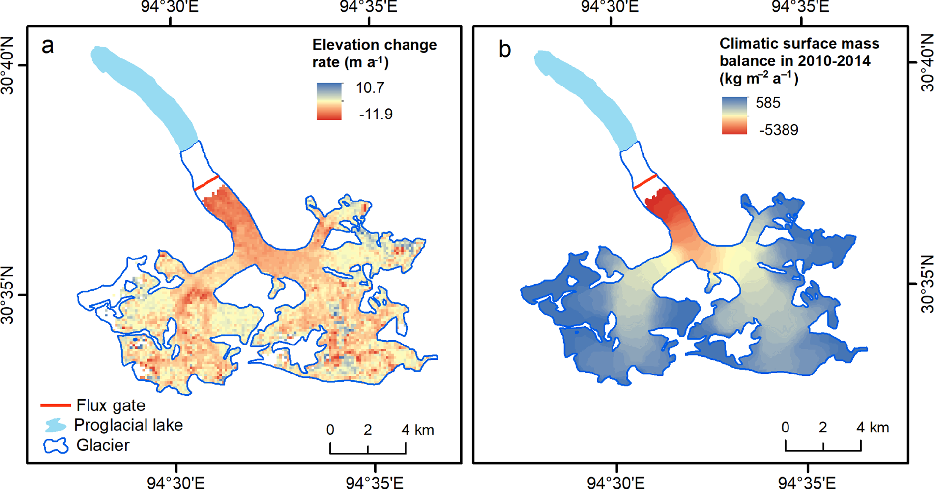
  $\left( {{Q_{{\text{in}}}} - {Q_{{\text{out}}}}} \right)/A$ (Cuffey and Paterson, Reference Cuffey and Paterson2010, Section 4.7). During 2010–2014, the geodetic mass balance over the calibration section, derived from Hugonnet and others (Reference Hugonnet2021), was −830 kg m−2 a−1 (Fig. 4a). The dynamic contribution associated with ice flux divergence amounted to −100 kg m−2 a−1. After removing this dynamic component, the resulting climatic surface mass balance, representing the appropriate target for degree-day model calibration, was −730 kg m−2 a−1. The distributed degree-day mass-balance model yields a mean climatic surface mass balance of −736 kg m−2 a−1 during 2010–2014 over the same calibration section, in close agreement with the adjusted geodetic reference value (Fig. 4b). Calibration results indicated that the optimum
  ${\text{DD}}{{\text{F}}_{{\text{ice}}}}$ was 7.0 mm d−1 ℃−1 and
  ${\text{DD}}{{\text{F}}_{{\text{snow}}}}$ was 2.5 mm d−1 ℃−1 in the model, to simulate the mass balance of the Jiongpu Co Glacier during 2014–2015.

Figure 4. (a) Surface elevation change rate over the calibration section (glacier area above 4400 m) during 2010–2014, derived from Hugonnet and others (Reference Hugonnet2021). (b) Modeled surface mass balance of the Jiongpu Co Glacier during the calibration period (2010–2014) derived from the distributed degree-day mass-balance model. Colors indicate the spatial distribution of climatic surface mass balance (kg m−2 a−1) within the calibration region above 4400 m. The modeled annual surface mass balance averaged over the calibration region varies between −998 kg m−2 a−1 and −667 kg m−2 a−1, with a mean value of −736 kg m−2 a−1. The flux gate (red line) and the proglacial lake (light blue) are indicated.
Uncertainties in glacier mass change ( $E\_{M_t}$) primarily originate from three sources: surface velocity, mass balance and ice thickness. For mass-balance uncertainty, we estimated it based on the uncertainties in surface elevation change data. According to the error propagation law, the uncertainty of mass loss from lake-terminating glaciers was calculated using the following formulas (Kochtitzky and others, Reference Kochtitzky2022):
 \begin{align}E\_{D_{{\text{ice}}}}^2 &= {\left( {{\rho _{{\text{ice}}}} \cdot t \cdot {{\bar h}_{\text{F}}} \cdot D \cdot {\sigma _{\bar v}}} \right)^2} \nonumber \\
&+ {\left( {{\rho _{{\text{ice}}}} \cdot \bar v \cdot t \cdot D \cdot {\sigma _{{{\bar h}_F}}}} \right)^2} + {\left( {{\rho _{{\text{ice}}}} \cdot \bar v \cdot t \cdot {{\bar h}_{\text{F}}} \cdot {\sigma _{\text{D}}}} \right)^2} \nonumber \\
&+ {\left( {t \cdot {S_{{\text{FT}}}} \cdot {\sigma _{{{\bar b}_{{\text{clim}}}}}}} \right)^2} + {\left( {t \cdot {{\bar b}_{{\text{clim}}}} \cdot {\sigma _{{{\text{S}}_{{\text{FT}}}}}}} \right)^2}\end{align}
\begin{align}E\_{D_{{\text{ice}}}}^2 &= {\left( {{\rho _{{\text{ice}}}} \cdot t \cdot {{\bar h}_{\text{F}}} \cdot D \cdot {\sigma _{\bar v}}} \right)^2} \nonumber \\
&+ {\left( {{\rho _{{\text{ice}}}} \cdot \bar v \cdot t \cdot D \cdot {\sigma _{{{\bar h}_F}}}} \right)^2} + {\left( {{\rho _{{\text{ice}}}} \cdot \bar v \cdot t \cdot {{\bar h}_{\text{F}}} \cdot {\sigma _{\text{D}}}} \right)^2} \nonumber \\
&+ {\left( {t \cdot {S_{{\text{FT}}}} \cdot {\sigma _{{{\bar b}_{{\text{clim}}}}}}} \right)^2} + {\left( {t \cdot {{\bar b}_{{\text{clim}}}} \cdot {\sigma _{{{\text{S}}_{{\text{FT}}}}}}} \right)^2}\end{align} \begin{align}E\_{M_{term}}^2 &= {\left( {{\rho _{ice}} \cdot {{\bar h}_{\Delta S}} \cdot {\sigma _{\Delta S}}} \right)^2} + {\left( {{\rho _{ice}} \cdot \Delta S \cdot {\sigma _{{{\bar h}_{\Delta S}}}}} \right)^2} \nonumber \\
&+ {\left( {0.5 \cdot t \cdot {{\bar b}_{clim\Delta S}} \cdot {\sigma _{\Delta S}}} \right)^2} + {\left( {0.5 \cdot t \cdot \Delta S \cdot {\sigma _{{{\bar b}_{clim\Delta S}}}}} \right)^2}{\text{ }}\end{align}
\begin{align}E\_{M_{term}}^2 &= {\left( {{\rho _{ice}} \cdot {{\bar h}_{\Delta S}} \cdot {\sigma _{\Delta S}}} \right)^2} + {\left( {{\rho _{ice}} \cdot \Delta S \cdot {\sigma _{{{\bar h}_{\Delta S}}}}} \right)^2} \nonumber \\
&+ {\left( {0.5 \cdot t \cdot {{\bar b}_{clim\Delta S}} \cdot {\sigma _{\Delta S}}} \right)^2} + {\left( {0.5 \cdot t \cdot \Delta S \cdot {\sigma _{{{\bar b}_{clim\Delta S}}}}} \right)^2}{\text{ }}\end{align} \begin{align}E\_{M_s}^2 &= {\left( {{S_{t2}} \cdot {\sigma _{{{\bar b}_{climt2}}}}} \right)^2} + {\left( {{{\bar b}_{climt2}} \cdot {\sigma _{{S_{t2}}}}} \right)^2} \nonumber \\
&+ {\left( {0.5 \cdot t \cdot {{\bar b}_{clim\Delta S}} \cdot {\sigma _{\Delta S}}} \right)^2} + {\left( {0.5 \cdot t \cdot \Delta S \cdot {\sigma _{{{\bar b}_{clim\Delta S}}}}} \right)^2}{\text{ }}\end{align}
\begin{align}E\_{M_s}^2 &= {\left( {{S_{t2}} \cdot {\sigma _{{{\bar b}_{climt2}}}}} \right)^2} + {\left( {{{\bar b}_{climt2}} \cdot {\sigma _{{S_{t2}}}}} \right)^2} \nonumber \\
&+ {\left( {0.5 \cdot t \cdot {{\bar b}_{clim\Delta S}} \cdot {\sigma _{\Delta S}}} \right)^2} + {\left( {0.5 \cdot t \cdot \Delta S \cdot {\sigma _{{{\bar b}_{clim\Delta S}}}}} \right)^2}{\text{ }}\end{align} \begin{equation}E\_{M_{\text{t}}}^2 = E\_{D_{{\text{ice}}}}^2 + E\_{M_{{\text{term}}}}^2 + E\_{M_{\text{s}}}^2.\end{equation}
 In the above formulas,  $E\_y$ represents the uncertainty of the variable
  $y$, calculated using standard error propagation, and
  ${\sigma _x}$ denotes the uncertainty (standard deviation) of variable
  $x$.
$x$.
The uncertainty in ice thickness at the flux gate (13.8 m) was assessed using the standard deviation of five individual ice thickness estimates from the study by Farinotti and others (Reference Farinotti2019), which integrates results from five different modeling approaches. Terminus ice thickness uncertainty (∼15 m) was calculated by errors related to the vertical accuracy of the TanDEM-X DEM and lake bathymetry. The uncertainty of the modeled climatic mass balance (25.9 kg m−2 a−1) was estimated based on the root-mean-square error (RMSE) between a subset of results from the Monte Carlo parameter calibration and the geodetic mass balance. Specifically, we selected all simulations with RMSEs less than 50 kg m−2 a−1 relative to the reference value. Accordingly, the uncertainties in frontal ablation and surface mass loss over the period from 17 October 2014 to 30 November 2015 were calculated as 10.23 × 10⁻³ Gt and 1.96 × 10⁻³ Gt, respectively. The total uncertainty in glacier mass loss during this period was 10.42 × 10⁻³ Gt (Tab. S2).
2.2.4. Glacier calving velocity
Mass loss of a lake-terminating glacier in the frontal region is closely related to the rate at which ice is delivered to the glacier terminus. The rate of change in glacier length can be defined as the difference between ice velocity at the glacier terminus and the frontal ablation rate, which includes the contributions of calving and melting mostly occurring below the water surface (Benn and Evans, Reference Benn and Evans2010). Subaqueous melting was not considered in this study because it is negligible for glaciers that terminus directly connected to a freshwater lake (Sugiyama and others, Reference Sugiyama2016; Zhang and others, Reference Zhang, Xu, Liu, Ding and Zhao2023). Thus, the calving velocity of lake-terminating glaciers can be estimated as the difference between ice velocity at the glacier front and glacier length change over time (Benn and others, Reference Benn, Warren and Mottram2007; Benn and Evans, Reference Benn and Evans2010). The equation is as follows:
 \begin{equation}{U_{\text{c}}} \approx {U_{\text{T}}} - \frac{{\partial L}}{{\partial t}}\end{equation}
where  ${U_{\text{c}}}$ is the calving velocity,
  ${U_{\text{T}}}$ denotes the vertically averaged glacier velocity,
  $L$ is the change in glacier length and
  $t$ is the time interval. The glacier ice velocity at the front (
 ${U_{\text{T}}}$) was obtained by dividing the ice discharge from the flux gate to the front in unit time by the cross-sectional area (
 ${A_{\text{m}}}$) along the glacier terminus (Fig. 3b) (Minowa and others, Reference Minowa, Sugiyama, Sakakibara and Skvarca2017).
3. Results and discussion
3.1. Evolution of Jiongpu Co Glacier
The Jiongpu Co Glacier retreated by approximately 2200 m between 2010 and 2020 (Fig. S4a). Notably, between 17 October 2014 and 30 November 2015, a dramatic retreat of about 800 m occurred in approximately 400 d, at an average rate of 2 m d−1. The Jiongpu Co Glacier showed the most significant glacier retreat between 26 March and 13 May 2015, with a retreat rate of 7.6 m d−1. During January and February 2015, the glacier remained relatively stable, with minor advance observed (Fig. 5a).

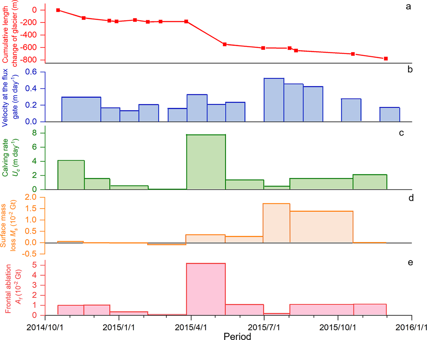
Figure 5. Jiongpu Co Glacier calving velocity ( ${U_{\text{c}}}$), cumulative length change, surface mass loss (
 ${M_{\text{s}}}$) and frontal ablation (
 ${A_{\text{f}}}$) from 17 October 2014 to 30 November 2015, and the velocity at glacier flux gate from 22 October 2014 to 16 December 2015.
Surface velocity extracted from the Sentinel-1 data shows that the average surface velocity of the entire glacier over the 400 d was 0.23 m d−1, which is faster than that of glaciers (0.06 m d−1) in the southeastern Tibetan (Zhang and others, Reference Zhang, Xu, Liu, Ding and Zhao2023). From glacier terminus to a distance of 8 km from the outlet of the lake, the average velocity during the investigated time period was approximately 0.41 m d−1. According to annual velocities obtained from ITS_LIVE V2, the average velocity at glacier terminus was 0.11 m d−1 before this dramatic retreat occurred (Fig. S4b). The average velocity of the Jiongpu Co Glacier was faster during July–September 2015 (Fig. 5b).
Between 17 October 2014 and 30 November 2015, the cumulative surface mass loss ( ${M_{\text{s}}}$) of Jiongpu Co Glacier was 3.9 × 10⁻² Gt, with interval values ranging from −0.01 × 10⁻² to 1.7 × 10⁻² Gt (Fig. 5d). Surface mass loss of Jiongpu Co Glacier was modest in boreal winter and markedly larger during the monsoon melt season, consistent with seasonal mass-balance patterns reported for glaciers in southeastern Tibet (Jouberton and others, Reference Jouberton2022).
Previous studies have shown that glaciers in the southeast Tibetan Plateau have retreated more slowly than the Jiongpu Co Glacier (Yao and others, Reference Yao2012; Wu and others, Reference Wu, Liu, Jiang, Xu, Wei and Guo2018; Zhang and others, Reference Zhang, Gao, Kang, Shangguan and Luo2021). The retreat rates of other glaciers in this region range from 2.7 to 69 m a−1 in 1980 to 2015, with the average value of 48.2 m a−1 from 1970s to 2000s (Yao and others, Reference Yao2012; Wang and others, Reference Wang, Che and Wei2021). Specifically, the lake-terminating Yanong glacier terminus retreated at a rate of only 13.6 m a−1 in 2000–2014 (Wu and others, Reference Wu, Liu, Jiang, Xu, Wei and Guo2018). The lake-terminating Lugge glacier in Bhutan Himalayas retreated 30–50 m a−1 in 2002 and 2003 (Naito and others, Reference Naito2012), which is also slower than Jiongpu Co Glacier. Thus, the retreat of the Jiongpu Co Glacier (approximately 800 m) marks the fastest retreat event on record on the Tibetan Plateau, comparable in magnitude to extreme cases like Upsala glacier’s 880 m a−1 retreat from January 2008 to May 2011 (Sakakibara and Sugiyama, Reference Sakakibara and Sugiyama2014).
3.2. Importance of calving in Jiongpu Co Glacier rapid retreat
For the Jiongpu Co Glacier, our observations revealed a temporal association between higher calving velocity and greater terminus retreat during the study period. From 17 October to 18 November 2014, the glacier exhibited a calving velocity of 4.1 m d−1, which caused glacier retreat of 125 m in total. Subsequently, glacier calving velocity decreased and glacier length changed minimally. The highest calving velocity occurred between 26 March and 13 May 2015, with a value of 7.8 m d−1. The largest change in glacier length (−365 m) also occurred during this period (Fig. 5). The rapid retreat of the Jiongpu Co Glacier during 2014–2015 was mostly caused by high calving velocity during March–May 2015. A previous study also suggested that the significant retreat of the lake-terminating glacier Bridge located in southwestern British Columbia since 1991 corresponded with rapid calving at the front (Chernos and others, Reference Chernos, Koppes and Moore2016). This evidence demonstrates that the calving velocity of a lake-terminating glacier directly determines the front position of the glacier.
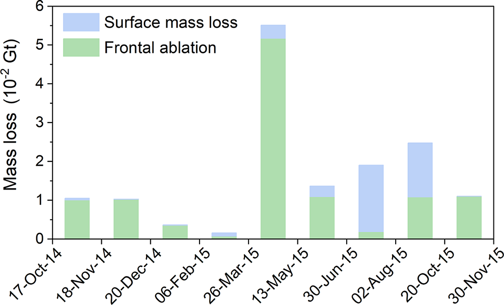
From 2010 to 2020, the average mass loss of Jiongpu Co Glacier was 5.5 × 10⁻² Gt a−1 due to frontal ablation and 5.1 × 10⁻² Gt a−1 due to surface mass loss (Zhao and others, Reference Zhao, Cheng, Guan, Zhang and Cao2024). However, from 17 October 2014 to 30 November 2015, the total mass loss reached 0.15 Gt, with the majority (74 ± 9%) contributed by frontal ablation due to calving (Fig. 6). Notably, the calving induced ablation in 2014–2015 was more than twice the average rate. The majority of this mass loss occurred from 26 March to 13 May 2015 (5.5 × 10⁻² Gt) and from 2 August to 20 October 2015 (2.5 × 10⁻² Gt), with 94 ± 12% and 43 ± 6% of the mass loss was contributed by frontal ablation, respectively. As a result, during the dramatic retreat of the Jiongpu Co Glacier, the mass loss intensified due to the high calving fluxes between March and May 2015.

Figure 6. Temporal evolution of surface mass loss and frontal ablation of the Jiongpu Co Glacier from 17 October 2014 to 30 November 2015.
3.3. Potential causes of the 2014–2015 rapid calving event
Between 2010 and 2020, the annual surface velocity along the glacier center flow line, within the segment between the terminus and the point located 8 km upstream of the Jiongpu Co Lake outlet, showed a fluctuating increasing trend, reaching a maximum in 2013 (Fig. S4b). Surface velocity acceleration around the glacier tongue enhances the longitudinal strain rate at the glacier front, leading to glacier stretching (Benn and others, Reference Benn, Warren and Mottram2007). Stretching of glaciers results in the formation of surface crevasses, which, when sufficiently deep, trigger calving at the glacier terminus (Benn and Evans, Reference Benn and Evans2010; Benn and others, Reference Benn2023). For example, the growth of surface crevasses at Sermeq Kujalleq glacier has been observed in the field and is associated with frequent calving events (Chudley and others, Reference Chudley, Christoffersen, Doyle, Abellan and Snooke2019; Cook and others, Reference Cook, Christoffersen, Truffer, Chudley and Abellán2021). The significant increase in annual velocity at the Jiongpu Co Glacier front in 2013 led to the emergence of surface crevasses in 2014, owing to continuous stretching (Fig. S5). Thus, accelerated glacier velocity was likely a key factor contributing to the rapid calving event observed during 2014–2015.
Certain studies have indicated that calving velocities tend to increase as glacier terminus approaches buoyancy (Benn and others, Reference Benn, Warren and Mottram2007; Dykes and others, Reference Dykes, Brook, Robertson and Fuller2011). In some calving laws, the calving velocity is inversely proportional to the ice thickness above buoyancy thickness at the glacier terminus, which is approximately 1.11 times as thick as the depth of freshwater lakes (Benn and Evans, Reference Benn and Evans2010). Although the Jiongpu Co Glacier has always been in a deep-water region, the ice thickness above the flotation thickness at the glacier terminus decreased from approximately 40 m in 2010 to 30 m in 2014 (Fig. 7). This reduction increased the buoyant forcing at the terminus, thereby facilitated calving during 2014–2015. Following the rapid retreat, the ice thickness above the buoyancy height at the terminus increased substantially, reaching an average of 81 m from 2016 to 2020 (Fig. S4c), which reduced the buoyancy and helped stabilize the terminus. As a result, the Jiongpu Co Glacier terminus remained relatively stable during 2016–2020, with a total retreat of 130 m (Zhao and others, Reference Zhao, Cheng, Guan, Zhang and Cao2024). Consistent with the observations at Jiongpu Co Glacier, the calving velocity of lake-terminating glaciers such as Tasman (New Zealand) and Mendenhall (Alaska) increased from 50 m a−1 to 227–431 m a−1 as buoyancy increased during their transition from grounded to floating termini (Boyce and others, Reference Boyce, Motyka and Truffer2007; Dykes and others, Reference Dykes, Brook, Robertson and Fuller2011). Therefore, the decrease in ice thickness above flotation at the glacier terminus was another key factor contributing to the rapid calving event of Jiongpu Co Glacier during 2014–2015.

Figure 7. Surface elevation and terminus position of Jiongpu Co Glacier in 2010, 2014 and 2015, with the distance starting from the outlet of lake. Glacier surface elevations were reconstructed using the DEM as a reference surface combined with geodetic elevation change rate from Hugonnet and others (Reference Hugonnet2021). The black dashed line indicates glacier terminus elevation when ice thickness at glacier front equals flotation thickness. The insert illustrates the relationship between lake depth and flotation height, as well as ice thickness condition of floating and grounded terminus. The bedrock topography of the glacier, represented by a dashed line, was obtained using SRTM DEM combined with ice thickness data from Farinotti and others (Reference Farinotti2019).
4. Conclusions and outlook
This study investigated the rapid retreat of the Jiongpu Co Glacier by approximately 800 m in the Tibetan Plateau during 2014–2015, which was a dramatic retreat event recorded on the Tibetan Plateau. The evolution of the lake and glacier during this year was meticulously delineated using multi-source remote sensing images. The main conclusions are as follows:
With rapid expansion of the lake in this period, the Jiongpu Co Glacier experienced a total mass loss of 0.15 ± 0.01 Gt, primarily attributed to frontal ablation (74 ± 9%). Specifically, the significant frontal ablation (5.2 × 10⁻² Gt) mainly caused by frontal calving occurred between March and May 2015, with a peak retreating rate of 7.6 m d−1. This indicates that during this rapid retreat event, rapid glacier calving was the primary driving force behind the rapid retreat.
In this study, we propose that the acceleration of terminus velocity at Jiongpu Co Glacier increased the longitudinal stretching force, leading to the formation of crevasses and promoting calving. At the same time, the thinning of ice reduced the terminus ice thickness above the buoyancy height from 40 m to 30 m, thereby increasing buoyancy and reducing basal friction. This thinning likely lowered the effective pressure at the glacier front, which in turn further accelerated glacier surface velocity, enhanced longitudinal stretching and destabilized the glacier terminus (Benn and others, Reference Benn, Warren and Mottram2007). We suggest that thinning and acceleration of glacier velocity at the glacier terminus may have interacted and contributed to the rapid calving events during 2014–2015.
While this study provides new insights into the mechanisms of rapid glacier retreat driven by frontal calving, it is limited by the lack of direct observations of basal and subaqueous conditions at the glacier terminus. In particular, the thermodynamic state at the ice–water interface remains insufficiently understood but may play a critical role in controlling calving processes. Future research combining in situ measurements and dynamic modeling is essential to better understand calving dynamics in lake-terminating glaciers.
Supplementary material
The supplementary material for this article can be found at https://doi.org/10.1017/jog.2026.10148.
Data availability statement
All data can be provided by the corresponding authors upon request.
Acknowledgements
We thank everyone who helped us with our fieldwork. This study was financially supported by the National Key Research and Development Program of China (Grant No.2024YFF0810700), National Natural Science Foundation of China (Grant No. 42071077), Science and technology Project of Tibet Autonomous Region (Grant No. XZ202501ZY0038).
Competing interests
The authors declare that they have no conflict of interest.


 Open access