


1. Introduction
The advent of wide-field interferometers such as the Murchison Widefield Array (MWA; Tingay et al. Reference Tingay2013; Wayth et al. Reference Wayth2018), Long Wavelength Array (Ellingson et al. Reference Ellingson2009) and the Low-Frequency Array (van Haarlem et al. Reference van Haarlem2013) has created a number of imaging challenges. These challenges include the large number of measurements in each observation, the instrumental effects that are measurement dependent, and the large image sizes due to high resolution and wide-field of view. Additionally, these telescopes have a variety of science goals, including high-priority science such as probing Galactic and extra-galactic magnetic fields (especially in low mass galaxy clusters; Johnston-Hollitt et al. Reference Johnston-Hollitt2015), and detecting the redshifted 21 cm spectral line of the Epoch of Reionoisation (Koopmans et al. Reference Koopmans2015). Furthermore, the wide-field of view provides the advantage of observing many objects in a single pointing, reducing the observation time needed to survey the radio sky. If the imaging challenges are overcome, it will herald an era of unprecedented sensitivity and resolution for the low-frequency sky, over extremely wide-field of views.
Non-coplanar baselines, (u, v, w), in the presence of wide-fields of view produce measurement dependent effects, i.e. a directional-dependent effect (DDE) that is different for each measurement. Each w value provides a complex exponential, known as a chirp, that needs to be modelled in the image domain and applied during image reconstruction. This has been through the use of two algorithms, the w-stacking algorithm, where average w corrections are applied in the image domain to groups of measurements, and the w-projection algorithm, where average w-corrections are applied when degridding in the (u, v, w) domain. The w-stacking algorithm (Humphreys & Cornwell Reference Humphreys and Cornwell2011) has the trade off that a Fast Fourier Transform (FFT) needs to be applied for each w group. The w-projection algorithm (Cornwell, Golap, & Bhatnagar Reference Cornwell, Golap, Bhatnagar, Shopbell, Britton and Ebert2005) has the trade off that kernel construction can be expensive and the support size is large for large w values. Both algorithms have been limited to correcting individual groups of measurements for large data sets (Cornwell et al. Reference Cornwell, Golap, Bhatnagar, Shopbell, Britton and Ebert2005; Offringa et al. Reference Offringa2014).
Two recent developments have allowed individual correction for each data sample. The first is the use of adaptive quadrature and radial symmetry to calculate w-projection kernels’ orders of magnitude faster than the full 2d calculation (Pratley, Johnston-Hollitt, & McEwen Reference Pratley, Johnston-Hollitt and McEwen2019c, hereafter Paper I). The second is the developments in distributed image reconstruction from state-of-the-art convex optimisation algorithms, which provide a natural framework for the Message Passing Interface (MPI) distribution of FFTs and degridding for radio interferometric imaging. Recently, an MPI hybrid w-stacking w-projection algorithm demonstrating these developments was applied on a super computing cluster, where 17.5 million measurements were individually corrected over a 25 by 25 degrees field of view from an MWA observation (Paper I). Such individual correction has not been previously possible.
After reviewing the w-stacking w-projection algorithm, we provide the algorithmic details of how to distribute the measurements through a k-means clustering algorithm to improve computational performance, the use of conjugate symmetry to reduce the range of w values, and show the application of these algorithms to a larger data set to demonstrate the improvement. We end with a discussion of future strategies for kernel calculation and adapting the algorithm to model other DDEs.
The paper is laid out as follows. Section 2 introduces the wide-field interferometric measurement equation. Section 3 describes the distributed k-means clustering algorithm used to create the w-stacks and the reconstruction algorithm used to generate a sky model of the observed data. Section 4 times and compares the w-stacking w-projection algorithm before and after using conjugate symmetry, as a function of image size, w-range, and number of visibilities. Section 5 demonstrates the application of the algorithm for this implementation on an observation of Fornax A. Section 6 proposes possible improvements in kernel calculation for large data sets and discusses how other DDEs can be included into the algorithm. The work is concluded in Section 7.
2. Wide-field imaging measurement equation
The non-coplanar wide-field interferometric measurement equation is
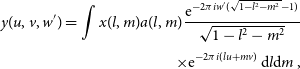 \begin{align} y(u, v, w^\prime) = \int x(l, m) a(l, m)\frac{{\rm e}^{-2\pi i w^\prime(\sqrt{1 -l^2 - m^2} - 1)}}{\sqrt{1 -l^2 - m^2}}\nonumber\\[3pt] \times {\rm e}^{-2\pi i (lu + mv)}\, {\rm d}l{\rm d}m\, , \end{align}
where  $(u, v, w^\prime)$
are the baseline coordinates and
$(u, v, w^\prime)$
are the baseline coordinates and  $(l, m, \sqrt{1 -l^2 -m^2})$
are directional cosines restricted to the upper unit sphere. In this work, we define
$(l, m, \sqrt{1 -l^2 -m^2})$
are directional cosines restricted to the upper unit sphere. In this work, we define  $w^\prime = w + \bar{w}$
, where
$w^\prime = w + \bar{w}$
, where  $\bar{w}$
is the average value of w-terms, w is the effective w-component (with zero mean), x is the sky brightness, and a includes DDEs such as the primary beam. The measurement equation is a mathematical model of the measurement process, i.e. signal acquisition, that allows one to calculate model measurements y when provided with a sky model x.
$\bar{w}$
is the average value of w-terms, w is the effective w-component (with zero mean), x is the sky brightness, and a includes DDEs such as the primary beam. The measurement equation is a mathematical model of the measurement process, i.e. signal acquisition, that allows one to calculate model measurements y when provided with a sky model x.
A number of methods can be used to solve for x given samples y, such as CLEAN (Högbom Reference Högbom1974), Maximum Entropy (Ables Reference Ables1974; Cornwell & Evans Reference Cornwell and Evans1985), and Sparse Regularisation algorithms (McEwen & Wiaux Reference McEwen and Wiaux2011; Onose et al. Reference Onose, Carrillo, Repetti, McEwen, Thiran, Pesquet and Wiaux2016; Pratley et al. Reference Pratley, McEwen, d’Avezac, Carrillo, Onose and Wiaux2018; Dabbech et al. Reference Dabbech, Onose, Abdulaziz, Perley, Smirnov and Wiaux2018; Pratley et al. Reference Pratley, Johnston-Hollitt and McEwen2019c). Ultimately, all interferometric measurement equations are derived from the van Cittert-Zernike theorem (Zernike Reference Zernike1938), and the measurement equation can be extended to include general DDEs and polarisation and to solve for x natively on the sphere (McEwen & Scaife Reference McEwen and Scaife2008; Smirnov Reference Smirnov2011; Price & Smirnov Reference Price and Smirnov2015).
To make use of the FFT, the measurement equation is traditionally calculated and approximated using degridding (Fessler & Sutton Reference Fessler and Sutton2003; Thompson, Moran, & Swenson Reference Thompson, Moran and Swenson2008). The measurement equation can be represented by the following linear operations
 \begin{equation} {\textit{y}} = {\textsf{WGCFZS}} {\textit{x}}\, . \end{equation} ${\textsf{S}}$
represents a gridding correction and correction of baseline independent effects such as
${\textsf{S}}$
represents a gridding correction and correction of baseline independent effects such as  $\bar{w}$
,
$\bar{w}$
,  ${\textsf{Z}}$
represents zero padding of the image,
${\textsf{Z}}$
represents zero padding of the image,  ${\textsf{F}}$
is an FFT,
${\textsf{F}}$
is an FFT,  ${\textsf{G}}$
represents a sparse circular convolution matrix that interpolates measurements off the grid and the combined
${\textsf{G}}$
represents a sparse circular convolution matrix that interpolates measurements off the grid and the combined  ${\textsf{G}}{\textsf{C}}$
includes baseline-dependent effects such as variations in the primary beam and w-component in the interpolation, and
${\textsf{G}}{\textsf{C}}$
includes baseline-dependent effects such as variations in the primary beam and w-component in the interpolation, and  ${\textsf{W}}$
are weights applied to the measurements. This linear operator is typically called a measurement operator
${\textsf{W}}$
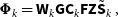
are weights applied to the measurements. This linear operator is typically called a measurement operator  ${\boldsymbol{\Phi}} = {\textsf{W}}{\textsf{G}}{\textsf{C}}{\textsf{F}}{\textsf{Z}}{\textsf{S}}$
with
${\boldsymbol{\Phi}} = {\textsf{W}}{\textsf{G}}{\textsf{C}}{\textsf{F}}{\textsf{Z}}{\textsf{S}}$
with  ${\boldsymbol{\Phi}} \in \mathbb{C}^{M \times N}$
, where there are N pixels and M visibilities. Furthermore,
${\boldsymbol{\Phi}} \in \mathbb{C}^{M \times N}$
, where there are N pixels and M visibilities. Furthermore,  ${\textit{x}}_i = x(l_i, m_i)$
and
${\textit{x}}_i = x(l_i, m_i)$
and  ${\textit{y}}_k = y(u_k, v_k, w_k)$
are discrete vectors in
${\textit{y}}_k = y(u_k, v_k, w_k)$
are discrete vectors in  $\mathbb{R}^{N \times 1}$
and
$\mathbb{R}^{N \times 1}$
and  $\mathbb{C}^{M \times 1}$
in this setting. The measurement operator has an adjoint operator
$\mathbb{C}^{M \times 1}$
in this setting. The measurement operator has an adjoint operator  ${\boldsymbol{\Phi}}^\dagger$
. The dirty map can be calculated by
${\boldsymbol{\Phi}}^\dagger$
. The dirty map can be calculated by  ${\boldsymbol{\Phi}}^\dagger{\textit{y}}$
, and the residual map by
${\boldsymbol{\Phi}}^\dagger{\textit{y}}$
, and the residual map by  $ {\boldsymbol{\Phi}}^\dagger{\textit{y}} - {\boldsymbol{\Phi}}^\dagger{\boldsymbol{\Phi}}{\textit{x}}$
.
$ {\boldsymbol{\Phi}}^\dagger{\textit{y}} - {\boldsymbol{\Phi}}^\dagger{\boldsymbol{\Phi}}{\textit{x}}$
.
3. Distributed wide-field imaging
In this section, we briefly describe the algorithmic details for the distributed w-projection w-stacking hybrid algorithm.
We use the interferometric image reconstruction software package PURIFYFootnote a (version 3.0.1, Pratley et al. Reference Pratley2019a) developed in C++ (Carrillo, McEwen, & Wiaux Reference Carrillo, McEwen and Wiaux2014; Pratley et al. Reference Pratley, McEwen, d’Avezac, Carrillo, Onose and Wiaux2018), where the authors have implemented an MPI-distributed measurement operator. The authors have also developed MPI-distributed wavelet transforms, along with MPI variations of the alternating direction method of multipliers (ADMM) algorithm in the software package SOPTFootnote b (version 3.0.1, Pratley et al. Reference Pratley2019b).
This is not the first time that sparse image reconstruction has been used for wide-fields of view. In particular, the w-term is known to spread information across visibilities, increasing the effective bandwidth in what is known as the spread spectrum effect (Dabbech et al. Reference Dabbech, Wolz, Pratley, McEwen and Wiaux2017; McEwen & Wiaux Reference McEwen and Wiaux2011; Wiaux et al. Reference Wiaux, Puy, Boursier and Vandergheynst2009; Wolz et al. Reference Wolz, McEwen, Abdalla, Carrillo and Wiaux2013), increasing the possible resolution of the reconstructed sky model. But these previous works have been restricted to proof-of-concept studies. One of the advantages of sparse image reconstruction algorithms, such as ADMM, is that they can allow direct reconstruction of an accurate sky model, unlike CLEAN-based algorithms that produce a restored image (Pratley et al. Reference Pratley, McEwen, d’Avezac, Carrillo, Onose and Wiaux2018).
3.1. w-projection w-stacking measurement operator
In the MPI w-stacking w-projection algorithm, the measurement operator corrects for the average w-value in each w-stack, then applies an extra correction to each visibility with the w-projection. Each w-stack  ${\textit{y}}_k$
has the measurement operator of
${\textit{y}}_k$
has the measurement operator of
 \begin{equation} {\boldsymbol{\Phi}}_k = {\textsf{W}}_k{\textsf{GC}}_k{\textsf{F}}{\textsf{Z}}{\tilde{{\textsf{S}}}}_k\,,\end{equation}
the gridding correction,  $\tilde{{\textsf{S}}}_k$
, has been modified to correct for the w-stack-dependent effects, such as the average
$\tilde{{\textsf{S}}}_k$
, has been modified to correct for the w-stack-dependent effects, such as the average  $\bar{w}_k$
or the primary beam
$\bar{w}_k$
or the primary beam
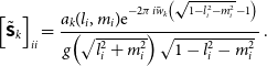 \begin{equation} \left[\tilde{{\textsf{S}}}_k\right]_{ii} = \frac{a_k(l_i, m_i){\rm e}^{-2\pi i \bar{w}_k\left(\sqrt{1 -l^2_i -m^2_i} - 1\right)}}{g\!\left(\sqrt{l^2_i + m^2_i}\right)\sqrt{1 -l^2_i - m^2_i}}\, .\end{equation}
We choose no primary beam effects within the stack  $a_k(l_i, m_i)$
.
$a_k(l_i, m_i)$
.  $g(\sqrt{l^2_i + m^2_i})$
is the window for the anti-aliasing filter. This gridding correction shifts the relative w value in the stack. This can reduce the effective w value in the stack, especially when the stack is close to the mean
$g(\sqrt{l^2_i + m^2_i})$
is the window for the anti-aliasing filter. This gridding correction shifts the relative w value in the stack. This can reduce the effective w value in the stack, especially when the stack is close to the mean  $\bar{w}_k$
, i.e. the value of
$\bar{w}_k$
, i.e. the value of  $w_i - \bar{w}_k$
is small for all i in stack k. This reduces the size of the support needed in the w-projection gridding kernel for each stack,
$w_i - \bar{w}_k$
is small for all i in stack k. This reduces the size of the support needed in the w-projection gridding kernel for each stack,
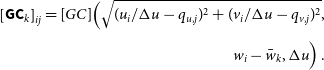 \begin{align} \left[{\textsf{GC}}_k\right]_{ij} = [GC]\Big(\sqrt{(u_i/\Delta u - q_{u, j})^2 + (v_i/\Delta u - q_{v, j})^2}, \nonumber\\[3pt] w_i - \bar{w}_k, \Delta u\Big)\, . \end{align} $(q_{u, j}, q_{v, j})$
represents the nearest grid points, and we use adaptive quadrature to calculate
$(q_{u, j}, q_{v, j})$
represents the nearest grid points, and we use adaptive quadrature to calculate
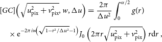 \begin{align} & [GC]\Big(\sqrt{u_{\rm pix}^2 + v_{\rm pix}^2}, w, \Delta u\Big) = \frac{2\pi}{\Delta u ^2}\int_{0}^{\alpha/2} g(r)\nonumber\\[3pt] &\quad \times{\rm e}^{-2\pi iw\!\left(\sqrt{ 1 - r^2/\Delta u^2} - 1\right)} J_0\left(2\pi r \sqrt{u_{\rm pix}^2 + v_{\rm pix}^2}\right) r{\rm d}r\, , \end{align}
where g(r) is the radial anti-aliasing filter,  $\Delta u$
is the resolution of the Fourier grid of the field of view zero padded by the oversampling ratio
$\Delta u$
is the resolution of the Fourier grid of the field of view zero padded by the oversampling ratio  $\alpha = 2$
, and
$\alpha = 2$
, and  $(u_{\rm pix},v_{\rm pix})$
are the pixel coordinates on the Fourier grid. More details can be found in Paper I.
$(u_{\rm pix},v_{\rm pix})$
are the pixel coordinates on the Fourier grid. More details can be found in Paper I.
For each stack  ${\textit{y}}_k \in \mathbb{C}^{M_k}$
, we have the measurement equation
${\textit{y}}_k \in \mathbb{C}^{M_k}$
, we have the measurement equation  ${\textit{y}}_k = {\boldsymbol{\Phi}}_k{\textit{x}}$
. It is clear that each stack has an independent measurement equation. However, the full measurement operator is related to the stacks in the adjoint operators such that
${\textit{y}}_k = {\boldsymbol{\Phi}}_k{\textit{x}}$
. It is clear that each stack has an independent measurement equation. However, the full measurement operator is related to the stacks in the adjoint operators such that
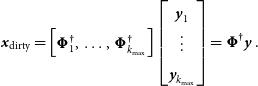 \begin{equation} {\textit{x}}_{\rm dirty} = \begin{bmatrix}{\boldsymbol{\Phi}}_1^\dagger,& \dots, &{\boldsymbol{\Phi}}_{k_{\rm max}}^\dagger \end{bmatrix} \begin{bmatrix} {\textit{y}}_1 \\ \vdots \\ {\textit{y}}_{k_{\rm max}} \end{bmatrix} = {\boldsymbol{\Phi}}^\dagger {\textit{y}}\, .\end{equation}
We use MPI all reduce to sum over the dirty maps generated from each node. The full operator  ${\boldsymbol{\Phi}}$
is normalised using the power method.
${\boldsymbol{\Phi}}$
is normalised using the power method.
3.2. Clustering w-stacks
It is ideal to minimise the kernel sizes across all stacks, minimising the memory and computation costs of the kernel. We develop an MPI k-means clustering algorithm which greatly improves performance by reducing the values of  $|w_i - \bar{w}_k|^2$
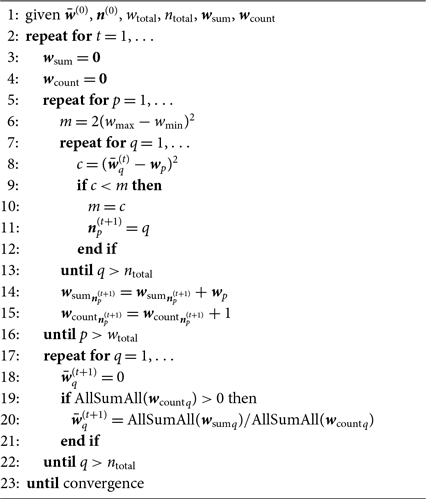
across the w-stacks. Each MPI node finds the w-stack to which a visibility belongs, updating the cluster centres across all MPI nodes with each iteration. This is then followed by an all-to-all MPI operation to distribute the visibilities to their w-stacks. There already exist parallel and distributed k-means clustering algorithms for big data (Aggarwal & Reddy Reference Aggarwal and Reddy2013; Stoffel & Belkoniene Reference Stoffel, Belkoniene, Amestoy, Berger, Daydé, Ruiz, Duff, Frayssé and Giraud1999). The k-means w-clustering algorithm is presented in Algorithm 1. This algorithm is necessary to reduce computation and operating memory when applying the w-projection kernels by reducing the support size of each kernel.
$|w_i - \bar{w}_k|^2$
across the w-stacks. Each MPI node finds the w-stack to which a visibility belongs, updating the cluster centres across all MPI nodes with each iteration. This is then followed by an all-to-all MPI operation to distribute the visibilities to their w-stacks. There already exist parallel and distributed k-means clustering algorithms for big data (Aggarwal & Reddy Reference Aggarwal and Reddy2013; Stoffel & Belkoniene Reference Stoffel, Belkoniene, Amestoy, Berger, Daydé, Ruiz, Duff, Frayssé and Giraud1999). The k-means w-clustering algorithm is presented in Algorithm 1. This algorithm is necessary to reduce computation and operating memory when applying the w-projection kernels by reducing the support size of each kernel.
k-means w-stacking: The k-means algorithm sorts the visibilities into clusters (w-stacks) by minimizing the average w deviation,  $(\bar{w} - w)^2$
, within each cluster. We use bold variables to denote an array, subscript to denote the array element and superscript to denote the iteration. The algorithm returns two arrays:
$(\bar{w} - w)^2$
, within each cluster. We use bold variables to denote an array, subscript to denote the array element and superscript to denote the iteration. The algorithm returns two arrays:  ${\textit{n}}$
is the array of indices that labels the w-stack for each visibility;
${\textit{n}}$
is the array of indices that labels the w-stack for each visibility;  ${\bar{w}}$
is the average w value within each w-stack. The algorithm requires a starting w-stack distribution
${\bar{w}}$
is the average w value within each w-stack. The algorithm requires a starting w-stack distribution  $\bar{{\textit{w}}}^{(0)}$
, which we choose to be evenly distributed between the minimum and maximum w-values. The algorithm should iterate until
$\bar{{\textit{w}}}^{(0)}$
, which we choose to be evenly distributed between the minimum and maximum w-values. The algorithm should iterate until  $\bar{{\textit{w}}}^{(t)}$
has converged, which we choose to be a relative difference of
$\bar{{\textit{w}}}^{(t)}$
has converged, which we choose to be a relative difference of  $10^{-3}$
. Note p is the index of visibility, q is the index for w-stacks, and c is the place holder for the minimum deviation for the visibility at index p. The
$10^{-3}$
. Note p is the index of visibility, q is the index for w-stacks, and c is the place holder for the minimum deviation for the visibility at index p. The  ${\rm AllSumAll}(x)$
operation is an MPI reduction of a summation followed by broadcasting the result to all compute nodes.
${\rm AllSumAll}(x)$
operation is an MPI reduction of a summation followed by broadcasting the result to all compute nodes.
3.3. Conjugate symmetry
Prior to w-stacking with the k-means algorithm, conjugate symmetry may be used to restrict the w-values onto the positive w-domain. The origin of the w-effect stems from the 3d Fourier transform of a spherical shell and a horizon window, with the w component probing the Fourier coefficient of the signal along the line of sight. The sky, the horizon window, the spherical shell, and the primary beam can all be interpreted as a real-valued signal. This provides a conjugate symmetry between  $-|w|$
and
$-|w|$
and  $+|w|$
, i.e.
$+|w|$
, i.e.
 \begin{equation} y^*(u, v, -|w|) = y(-u, -v, |w|)\, .\end{equation}
Properties of noise remain unchanged under conjugate symmetry, meaning that measurements can be restricted to positive w, i.e.  $w \in \mathbb{R}_+$
. Other modelled instrumental effects may need to be conjugated, which is only important when they are complex-valued signals. In particular, polarised signals, e.g. Stokes Q, U, and V, are independent real-valued signals. Thus, linear polarisation has a slightly different relation
$w \in \mathbb{R}_+$
. Other modelled instrumental effects may need to be conjugated, which is only important when they are complex-valued signals. In particular, polarised signals, e.g. Stokes Q, U, and V, are independent real-valued signals. Thus, linear polarisation has a slightly different relation
 \begin{equation} y^*_P(u, v, -|w|) = y_Q(-u, -v, |w|) - iy_U(-u, -v, |w|)\, ,\end{equation}
suggesting that the reflection should be done to the Stokes Q and U visibliities before combination into linear polarisation and then combined with  $-i$
rather than
$-i$
rather than  $+i$
. This combination is important for accurate polarimetirc image reconstruction (Pratley & Johnston-Hollitt Reference Pratley and Johnston-Hollitt2016).
$+i$
. This combination is important for accurate polarimetirc image reconstruction (Pratley & Johnston-Hollitt Reference Pratley and Johnston-Hollitt2016).
3.4. Distributed ADMM
As in Paper I, we use the alternating direction method of multipliers (ADMM) algorithm implemented in PURIFY (Pratley et al. Reference Pratley, McEwen, d’Avezac, Carrillo, Onose and Wiaux2018) to solve the optimisation problem
 \begin{equation} \min_{{{\textit{x}}} \in \mathbb{R}^N}\big\| {\boldsymbol{\Psi}}^\dagger {{\textit{x}}} \big\|_{\ell_1}\quad {\rm subject}\, {\rm to} \quad \left \|{\textit{y}} - {\boldsymbol{\Phi}} {{\textit{x}}} \right\|_{\ell_2} \leq \epsilon\, ,\end{equation}
where  ${\boldsymbol{\Psi}}$
is a wavelet transform, the term
${\boldsymbol{\Psi}}$
is a wavelet transform, the term  $\big\| {\boldsymbol{\Psi}}^\dagger {{\textit{x}}} \big\|_{\ell_1}$
is a penalty on the number of non-zero wavelet coefficients, while
$\big\| {\boldsymbol{\Psi}}^\dagger {{\textit{x}}} \big\|_{\ell_1}$
is a penalty on the number of non-zero wavelet coefficients, while  ${\left \|{\textit{y}} - {\boldsymbol{\Phi}} {{\textit{x}}} \right\|_{\ell_2} \leq \epsilon}$
is the condition that the measurements fit within a Gaussian error bound
${\left \|{\textit{y}} - {\boldsymbol{\Phi}} {{\textit{x}}} \right\|_{\ell_2} \leq \epsilon}$
is the condition that the measurements fit within a Gaussian error bound  $\epsilon$
. MPI is used to distribute the wavelet transform and enforce fidelity constraints, in conjunction with w-stacking.
$\epsilon$
. MPI is used to distribute the wavelet transform and enforce fidelity constraints, in conjunction with w-stacking.
PURIFY (version 3.0.1, Pratley et al. Reference Pratley2019a) has been updated to implement the w-stacking w-projection measurement operator with MPI, k-means clustering, and conjugate symmetry to efficiently reduce the effective w-value within a compute cluster. We find that the use of conjugate symmetry allows the k-means algorithm to increase the density of the w-stack locations. This in turn reduces the effective w values that are required to be corrected for by the w-projection kernels and greatly decreases the computational burden of the w-projection algorithm in the kernel construction.
4. Efficiency of w-stacking with conjugate symmetry
In this section, we compare the efficiency of the w-projection w-stacking algorithm before and after applying conjugate symmetry to the visibilities. By restricting w to be greater than zero through conjugation, we increase the density of the w-stacks and decrease the distance  $|w - \bar{w}_k|$
of each visibility from the centre of a given w-stack k. When this distance is negligible, the correction required by the w-projection algorithm is also negligible.
$|w - \bar{w}_k|$
of each visibility from the centre of a given w-stack k. When this distance is negligible, the correction required by the w-projection algorithm is also negligible.
Each visibility in a w-stack has the remaining directional-dependent complex-phase variation
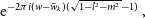 \begin{equation} {\rm e}^{-2\pi i (w - \bar{w}_k)(\sqrt{1 - l^2 - m^2} - 1)} \, ,\end{equation}
this can be accounted for using the w-projection algorithm. Otherwise, the remaining DDE oscillates across the field of view as a multiplicative phase error that is not accounted for. We use the inequality  $| 1 -e^{iq}| = 2 |\sin(q/2)| < |q|$
to provide a linear bound on the error within a w-stack
$| 1 -e^{iq}| = 2 |\sin(q/2)| < |q|$
to provide a linear bound on the error within a w-stack
 \begin{equation} \begin{split} |1 - {\rm e}^{-2\pi i (w - \bar{w}_k)(\sqrt{1 - l^2 - m^2} - 1)}| \qquad\qquad\quad\\[3pt] \leq|2\pi (w - \bar{w}_k)(\sqrt{1 - l^2 - m^2} - 1)| \, , \end{split}\end{equation}
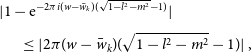
where the error is bounded by  $|2\pi (w_{\rm max} - w_{\rm min})(\sqrt{1 - l^2 - m^2} - 1)|$
for each stack. When the phase term is small, the bound closely approximates the error; this follows the standard small angle approximation commonly applied to the
$|2\pi (w_{\rm max} - w_{\rm min})(\sqrt{1 - l^2 - m^2} - 1)|$
for each stack. When the phase term is small, the bound closely approximates the error; this follows the standard small angle approximation commonly applied to the  $\sin$
function. We next use this error bound to estimate how many stacks are needed for a phase error tolerance over a field of view during wide-field corrections. We then show that application of conjugate symmetry can increase w-stacking efficiency by decreasing the w range.
$\sin$
function. We next use this error bound to estimate how many stacks are needed for a phase error tolerance over a field of view during wide-field corrections. We then show that application of conjugate symmetry can increase w-stacking efficiency by decreasing the w range.
When the w-stacks are evenly spread (which is expected to give rise to larger error than k-means for many of the stacks, see Figure 1), we know that the w term is uniformly bounded to be within a stack following the relation  $|w - \bar{w}_k| \leq |(w_{\rm max} - w_{\rm min})/n_{\rm d}|$
, where
$|w - \bar{w}_k| \leq |(w_{\rm max} - w_{\rm min})/n_{\rm d}|$
, where  $n_{\rm d}$
is the number of w-stacks. The field of view is limited through
$n_{\rm d}$
is the number of w-stacks. The field of view is limited through  $l_{\rm max} \geq \sqrt{l^2 + m^2}$
; this is determined by the resolution of the Fourier grid directly by
$l_{\rm max} \geq \sqrt{l^2 + m^2}$
; this is determined by the resolution of the Fourier grid directly by  $l_{\rm max} = \frac{1}{2\Delta u}$
. We denote our error tolerance for the multiplicative phase error across the field of view as
$l_{\rm max} = \frac{1}{2\Delta u}$
. We denote our error tolerance for the multiplicative phase error across the field of view as  ${\rm e}^{i\eta}$
. The number of w-stacks
${\rm e}^{i\eta}$
. The number of w-stacks  $n_{\rm d}$
is then constrained by
$n_{\rm d}$
is then constrained by
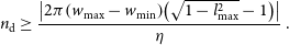 \begin{equation} n_{\rm d} \geq \frac{\left|2\pi \!\left(w_{\rm max} - w_{\rm min}\right)\!\left(\sqrt{1 - l_{\rm max}^2} - 1\right)\right|}{\eta} \, .\end{equation}
For example, if we allow for a multiplicative phase error of at most of  $\eta = 2\pi\times 0.1$
, then for a range of
$\eta = 2\pi\times 0.1$
, then for a range of  $|w_{\rm max} - w_{\rm min}| = 300$
wavelengths and a 30 degree radius of
$|w_{\rm max} - w_{\rm min}| = 300$
wavelengths and a 30 degree radius of  $l_{\rm max} = 0.5$
, we calculate that approximately
$l_{\rm max} = 0.5$
, we calculate that approximately  $n_{\rm d} = 400$
w-stacks are needed.
$n_{\rm d} = 400$
w-stacks are needed.
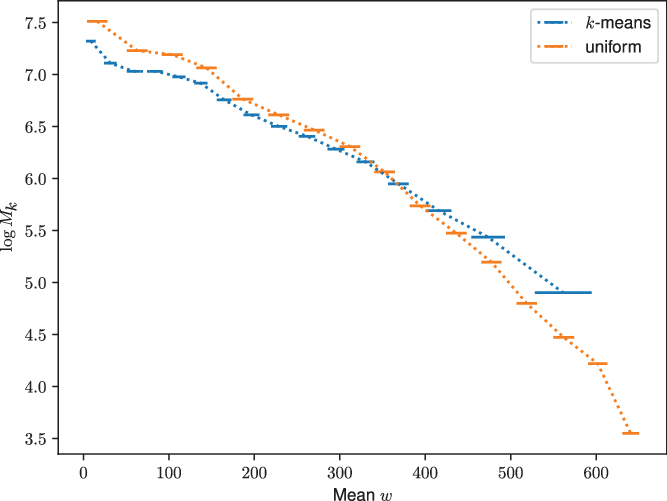
The number of visibilities per w-stack in log scale  $\log M_k$
as a function of mean w compared between using the k-means algorithm and uniform binning for 16 stacks. The horizontal error bars show the root-mean-squared w offset for the visibilities in a w-stack; this is proportional to the phase error that needs to be corrected due to the w-term. In particular, the k-means stacks show less residual w where there are more visibilities. To generate this plot, we used the Phase I MWA configuration after applying conjugation to ensure that all
$\log M_k$
as a function of mean w compared between using the k-means algorithm and uniform binning for 16 stacks. The horizontal error bars show the root-mean-squared w offset for the visibilities in a w-stack; this is proportional to the phase error that needs to be corrected due to the w-term. In particular, the k-means stacks show less residual w where there are more visibilities. To generate this plot, we used the Phase I MWA configuration after applying conjugation to ensure that all  $w \geq 0$
. We used a coverage from 768 channels with a width of 40 kHz centred at 87.68 MHz and a pointing centre 45 degree away from zenith towards the horizon. The k-means algorithm places less bins at larger values of w where there are less visibilities and conversely increases the number of bins at small w values where there are more visibilities. This has two possible advantages that the computational load is more balanced and that the w-offsets are reduced for the majority of the visibilities.
$w \geq 0$
. We used a coverage from 768 channels with a width of 40 kHz centred at 87.68 MHz and a pointing centre 45 degree away from zenith towards the horizon. The k-means algorithm places less bins at larger values of w where there are less visibilities and conversely increases the number of bins at small w values where there are more visibilities. This has two possible advantages that the computational load is more balanced and that the w-offsets are reduced for the majority of the visibilities.
However, the bound on the multiplicative phase error  $\eta$
due to the w-term might not be the greatest limitation. Long baselines at low frequencies can be limited by the ionospheric phase errors introduced during an observation.
$\eta$
due to the w-term might not be the greatest limitation. Long baselines at low frequencies can be limited by the ionospheric phase errors introduced during an observation.
When we use conjugate symmetry to ensure that  $w \geq 0$
, we find that the difference |
$w \geq 0$
, we find that the difference | $w_{\rm max} - w_{\rm min}|$
is reduced to
$w_{\rm max} - w_{\rm min}|$
is reduced to  ${\rm max}(|w|) - {\rm min}(|w|)$
. This reduces the number of w-stacks
${\rm max}(|w|) - {\rm min}(|w|)$
. This reduces the number of w-stacks  $n_{\rm d}$
required to reach a desired level of accuracy over the image, suggesting the efficiency increase. For example, after applying conjugate symmetry to a uniform w coverage with
$n_{\rm d}$
required to reach a desired level of accuracy over the image, suggesting the efficiency increase. For example, after applying conjugate symmetry to a uniform w coverage with  $w_{\rm max} = - w_{\rm min}$
, only half the number of stacks are needed for the same phase error bound. Furthermore, we note that the k-means algorithm can also provide more accuracy for less computation; this is shown in Figure 1 for an MWA uv-coverage.
$w_{\rm max} = - w_{\rm min}$
, only half the number of stacks are needed for the same phase error bound. Furthermore, we note that the k-means algorithm can also provide more accuracy for less computation; this is shown in Figure 1 for an MWA uv-coverage.
We also estimate that the 2-dimensional support size within a w-stack will be bounded by the maximum of  ${(2\Delta w_k/\Delta u)^2}$
and
${(2\Delta w_k/\Delta u)^2}$
and  $J^2$
, where J is the number of kernel coefficients used. Thus, it is clear that more efficient placements of w-stacks reduce memory and computation needed with the w-projection kernel. For uniform coverage, we expect that the number of 2d kernel coefficients is bounded by
$J^2$
, where J is the number of kernel coefficients used. Thus, it is clear that more efficient placements of w-stacks reduce memory and computation needed with the w-projection kernel. For uniform coverage, we expect that the number of 2d kernel coefficients is bounded by  ${(2(w_{\rm max} - w_{\rm min})/(n_{\rm d}\Delta u))^2}$
. This bound on support is further reduced to
${(2(w_{\rm max} - w_{\rm min})/(n_{\rm d}\Delta u))^2}$
. This bound on support is further reduced to  ${(2({\rm max}(|w|) - {\rm min}(|w|))/(n_{\rm d}\Delta u))^2}$
when conjugate symmetry is applied.
${(2({\rm max}(|w|) - {\rm min}(|w|))/(n_{\rm d}\Delta u))^2}$
when conjugate symmetry is applied.
Lastly, when  $\eta \geq |2\pi (w - \bar{w}_k)(\sqrt{1 - l_{\rm max}^2} - 1)|$
for a chosen tolerance and given visibility, we suggest that there is little advantage in using the w-projection kernel. There may be small gains in kernel construction time by assuming
$\eta \geq |2\pi (w - \bar{w}_k)(\sqrt{1 - l_{\rm max}^2} - 1)|$
for a chosen tolerance and given visibility, we suggest that there is little advantage in using the w-projection kernel. There may be small gains in kernel construction time by assuming  $w = \bar{w}_k$
to avoid calculating the w-projection kernel through adaptive quadrature when the Hankel transform of g(r) has a closed form. From the work of Pratley et al. (Reference Pratley, Johnston-Hollitt and McEwen2019c), a safe choice to bound the error is
$w = \bar{w}_k$
to avoid calculating the w-projection kernel through adaptive quadrature when the Hankel transform of g(r) has a closed form. From the work of Pratley et al. (Reference Pratley, Johnston-Hollitt and McEwen2019c), a safe choice to bound the error is  $\eta = 0.01$
but we expect this to be very conservative for most science cases. In the limit where the stacking density is high enough, this method then reduces to the standard w-stacking algorithm.
$\eta = 0.01$
but we expect this to be very conservative for most science cases. In the limit where the stacking density is high enough, this method then reduces to the standard w-stacking algorithm.
4.1. Comparison
In this section, we show the increase in efficiency of the construction and application of the measurement operator using the w-projection and w-stacking algorithm before and after applying conjugate symmetry to the visibilities.
To compare the efficiency, we undertake a series of timing experiments using a range of images sizes, w-stacks, and number of visibilities.
To perform the reconstruction, we used the Grace computing cluster at University College London. Each node of Grace contains two 8 core Intel Xeon E5-2630v3 processors (16 cores total) and 64 Gigabytes of RAM.Footnote c
Each data point was generated using 25 compute nodes and 25 w-stacks (i.e. one w-stack per node). The coverage was generated randomly using a Gaussian sampling density in u, v, and w. We choose the standard deviation of w to be 100 wavelengths, making the full range to be approximately  $\pm 300$
wavelengths. The field of view was kept fixed to 25 by 25 degrees, while we vary the range of w, number of pixels (N), and number of visibilities (M). We repeated each timing measurement thrice and then recorded the average time for each experimental configuration. We used an oversampling ratio of
$\pm 300$
wavelengths. The field of view was kept fixed to 25 by 25 degrees, while we vary the range of w, number of pixels (N), and number of visibilities (M). We repeated each timing measurement thrice and then recorded the average time for each experimental configuration. We used an oversampling ratio of  $\alpha = 2$
, with a 2d kernel support size
$\alpha = 2$
, with a 2d kernel support size  $J^2 = 16$
at
$J^2 = 16$
at  $w = 0$
. The number of kernel coefficients used for
$w = 0$
. The number of kernel coefficients used for  $|w| > 0$
is
$|w| > 0$
is  $\beta (w_i - \bar{w}_k)/\Delta u$
along each dimension (Pratley et al. Reference Pratley, Johnston-Hollitt and McEwen2019c), where
$\beta (w_i - \bar{w}_k)/\Delta u$
along each dimension (Pratley et al. Reference Pratley, Johnston-Hollitt and McEwen2019c), where  $\beta$
is a constant of proportionality. Here, we choose
$\beta$
is a constant of proportionality. Here, we choose  $\beta = 2$
; however, Cornwell, Golap, & Bhatnagar (Reference Cornwell, Golap and Bhatnagar2008) suggest that
$\beta = 2$
; however, Cornwell, Golap, & Bhatnagar (Reference Cornwell, Golap and Bhatnagar2008) suggest that  $\beta = \frac{\lambda}{D}$
is a good choice because of its relation to the Fresnel zone for a dish of size D. The choice of
$\beta = \frac{\lambda}{D}$
is a good choice because of its relation to the Fresnel zone for a dish of size D. The choice of  $\beta$
is dependent on the observational regime under consideration,Footnote d and the total number of coefficients scales as
$\beta$
is dependent on the observational regime under consideration,Footnote d and the total number of coefficients scales as  $(2 (w_i - \bar{w}_k)/\Delta u)^2$
. The standard deviation of the w sample density is determined by the value
$(2 (w_i - \bar{w}_k)/\Delta u)^2$
. The standard deviation of the w sample density is determined by the value  $\sigma_w$
, which we chose values of 50, 100, and 150 wavelengths, with maximum w values of
$\sigma_w$
, which we chose values of 50, 100, and 150 wavelengths, with maximum w values of  $\pm 3\sigma_w$
. Figure 2 shows the time required to construct the measurement operator
$\pm 3\sigma_w$
. Figure 2 shows the time required to construct the measurement operator  ${\boldsymbol{\Phi}}$
and apply
${\boldsymbol{\Phi}}$
and apply  ${\boldsymbol{\Phi}}^\dagger{\boldsymbol{\Phi}}$
as a function of image size, for
${\boldsymbol{\Phi}}^\dagger{\boldsymbol{\Phi}}$
as a function of image size, for  $N = 256^2, 512^2, 1\,024^2, 2\,048^2,$
and
$N = 256^2, 512^2, 1\,024^2, 2\,048^2,$
and  $4\,096^2$
pixels, and
$4\,096^2$
pixels, and  $M = 10^6, 10^7,$
and
$M = 10^6, 10^7,$
and  $10^8$
visibilities. All w-projection kernels are stored across the cluster to be ready for application.
$10^8$
visibilities. All w-projection kernels are stored across the cluster to be ready for application.
The left column shows plots of measurement operator ( ${\boldsymbol{\Phi}}$
) construction times, and the right column shows plots of
${\boldsymbol{\Phi}}$
) construction times, and the right column shows plots of  ${\boldsymbol{\Phi}}^\dagger{\boldsymbol{\Phi}}$
application times, as a function of image size N. The top, middle, and bottom rows show the times when using
${\boldsymbol{\Phi}}^\dagger{\boldsymbol{\Phi}}$
application times, as a function of image size N. The top, middle, and bottom rows show the times when using  $M = 10^6, 10^7, 10^8$
visibilities. The standard deviation of the w sample density is determined by the value
$M = 10^6, 10^7, 10^8$
visibilities. The standard deviation of the w sample density is determined by the value  $\sigma_w$
, which we chose values of 50, 100, and 150 wavelengths. We show results before and after applying conjugate symmetry to the visibilities. We find improvements in performance for large w ranges due to an increase in w-stacking efficiency, as described in Section 4. The kernel construction time is independent of image size due to the use of adaptive quadrature; this is clear for large M in the middle and bottom rows. For
$\sigma_w$
, which we chose values of 50, 100, and 150 wavelengths. We show results before and after applying conjugate symmetry to the visibilities. We find improvements in performance for large w ranges due to an increase in w-stacking efficiency, as described in Section 4. The kernel construction time is independent of image size due to the use of adaptive quadrature; this is clear for large M in the middle and bottom rows. For  $\sigma_w = 150$
wavelengths with
$\sigma_w = 150$
wavelengths with  $M = 10^8$
, we found that not applying conjugation resulted in large kernel construction times of greater than 140 min (not shown). We found construction time reduces to 30 min after applying conjugation as shown in the figure.
$M = 10^8$
, we found that not applying conjugation resulted in large kernel construction times of greater than 140 min (not shown). We found construction time reduces to 30 min after applying conjugation as shown in the figure.
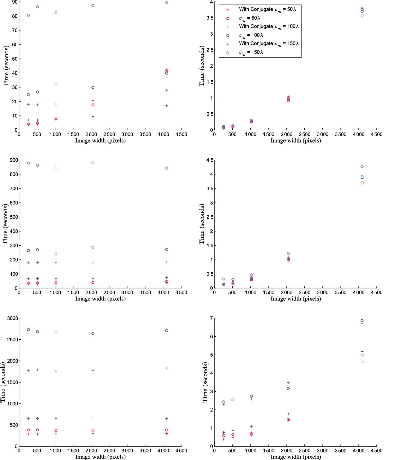
For constructing  ${\boldsymbol{\Phi}}$
, we find that kernel construction time is independent of image size, which is clear when the kernel construction dominates over the cost of planning the FFT. This demonstrates the advantage of using adaptive quadrature during kernel construction for high-resolution images, where the computation scales with the field of view and w only, leaving it completely independent of number of pixels in the image.
${\boldsymbol{\Phi}}$
, we find that kernel construction time is independent of image size, which is clear when the kernel construction dominates over the cost of planning the FFT. This demonstrates the advantage of using adaptive quadrature during kernel construction for high-resolution images, where the computation scales with the field of view and w only, leaving it completely independent of number of pixels in the image.
For  $\sigma_w = 50$
, we find that there is little improvement when applying conjugate symmetry, which is easily explained by suggesting that 25 w-stacks are enough to efficiently cover the range of w values over
$\sigma_w = 50$
, we find that there is little improvement when applying conjugate symmetry, which is easily explained by suggesting that 25 w-stacks are enough to efficiently cover the range of w values over  $[-150, 150]$
and [0, 150] wavelengths.
$[-150, 150]$
and [0, 150] wavelengths.
For the larger w ranges of  $\sigma_w = 100$
and
$\sigma_w = 100$
and  $\sigma_w = 150$
, we find that applying conjugate symmetry to the visibilities increases the efficiency of the w-stacking density. This reduces the w-projection kernel size, improving the construction speed of the w-projection kernels considerably. Kernel construction is approximately five times faster after applying conjugation. The reduced w-kernel size also reduces the time required to perform degridding and gridding operations during image reconstruction. However, as mentioned in the previous section, these performance gains are only seen if there are many visibilities with
$\sigma_w = 150$
, we find that applying conjugate symmetry to the visibilities increases the efficiency of the w-stacking density. This reduces the w-projection kernel size, improving the construction speed of the w-projection kernels considerably. Kernel construction is approximately five times faster after applying conjugation. The reduced w-kernel size also reduces the time required to perform degridding and gridding operations during image reconstruction. However, as mentioned in the previous section, these performance gains are only seen if there are many visibilities with  $w < 0$
.
$w < 0$
.
For  $\sigma_w = 150$
with
$\sigma_w = 150$
with  $M = 10^8$
, we found that not applying conjugation resulted in large kernel construction times of greater than 140 min and we did not have the compute resources to measure this as a function of N. However, applying conjugation significantly reduced construction times to 30 min.
$M = 10^8$
, we found that not applying conjugation resulted in large kernel construction times of greater than 140 min and we did not have the compute resources to measure this as a function of N. However, applying conjugation significantly reduced construction times to 30 min.
In Figure 3, we fixed the image size to be small  $N = 256^2$
and measured construction and application times for
$N = 256^2$
and measured construction and application times for  $M = 10^6, 10^7$
, and
$M = 10^6, 10^7$
, and  $10^8$
. We find that there is linear scaling in construction time as a function of M. The application times also increase with M, but it is not clear that it is linear.
$10^8$
. We find that there is linear scaling in construction time as a function of M. The application times also increase with M, but it is not clear that it is linear.
The left figure shows plots of measurement operator ( ${\boldsymbol{\Phi}}$
) construction times, and the right figure shows plots of
${\boldsymbol{\Phi}}$
) construction times, and the right figure shows plots of  ${\boldsymbol{\Phi}}^\dagger{\boldsymbol{\Phi}}$
application times, as a function of the number of visibilities M for
${\boldsymbol{\Phi}}^\dagger{\boldsymbol{\Phi}}$
application times, as a function of the number of visibilities M for  $N = 256^2$
. The standard deviation of the w sample density is determined by the value
$N = 256^2$
. The standard deviation of the w sample density is determined by the value  $\sigma_w$
, which we chose values of 50, 100, and 150 wavelengths. We find that the kernel construction time increases linearly with M. We find that the applying the conjugate consistently reduces the time required to calculate the w-projection kernels and can reduce the time for application.
$\sigma_w$
, which we chose values of 50, 100, and 150 wavelengths. We find that the kernel construction time increases linearly with M. We find that the applying the conjugate consistently reduces the time required to calculate the w-projection kernels and can reduce the time for application.
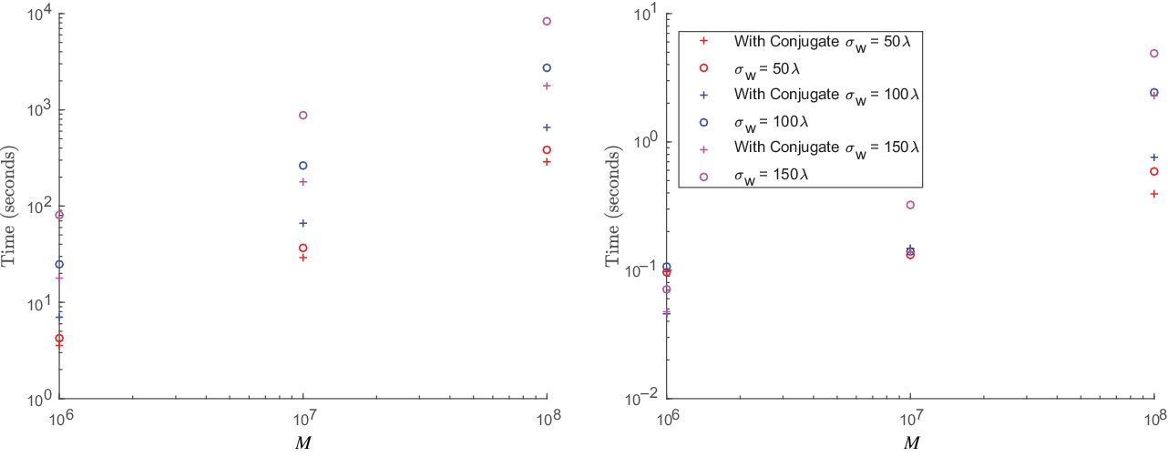
We also find that in the time to apply the measurement operator, the FFT scales with image width  $\sqrt{N}$
, and the contribution from the application of the gridding and degridding kernels that grows with M. This is expected from the two contributions
$\sqrt{N}$
, and the contribution from the application of the gridding and degridding kernels that grows with M. This is expected from the two contributions  $\mathcal{O}(M) $
and
$\mathcal{O}(M) $
and  $\mathcal{O}(\alpha^2 N \log \alpha^2 N)$
for the interpolation and FFT, respectively. However, we expect that the application time is limited by the node with the most measurements. Also the varying kernel support sizes make it difficult to expect a clear relation for application time against the number of measurements.
$\mathcal{O}(\alpha^2 N \log \alpha^2 N)$
for the interpolation and FFT, respectively. However, we expect that the application time is limited by the node with the most measurements. Also the varying kernel support sizes make it difficult to expect a clear relation for application time against the number of measurements.
4.2. Current implementation limitations
While we have shown performance improvements with this work, there are still limitations with the current implementation. We note that some of these limitations can be overcome. First, we pre-compute and store all of the kernels for use during image reconstruction. While this is fine for short snapshot observations, it requires a large amount of working memory and we expect that on-the-fly calculation methods proposed later in this work may prove useful (see Section 6). Second, this implementation is bottlenecked in working memory and CPU resources by the node with the w-stack that contains the largest number of gridding kernel coefficients.
5. Application to MWA observation of Fornax A
We use PURIFY (version 3.0.1, Pratley et al. Reference Pratley2019a) to perform wide-field image reconstruction of an observation of Fornax A taken with the MWA. The observation has a pointing centre of 03 $^\circ$
22ʹ 41.7ʹʹ −37
$^\circ$
22ʹ 41.7ʹʹ −37 $^\circ$
12ʹ 30ʹʹ, and the integration time is 112 s. Fornax A was observed using XX and YY polarisations, with the visibilities transformed into Stokes I. The bandwidth was 30.72 MHz with a central frequency of 184.955 MHz and using 768 channels, which is a standard observational mode for the MWA (Ord et al. Reference Ord2015; Prabu et al. Reference Prabu2015). The data reduction, including flagging and calibration, is as per McKinley et al. (Reference McKinley2015).
$^\circ$
12ʹ 30ʹʹ, and the integration time is 112 s. Fornax A was observed using XX and YY polarisations, with the visibilities transformed into Stokes I. The bandwidth was 30.72 MHz with a central frequency of 184.955 MHz and using 768 channels, which is a standard observational mode for the MWA (Ord et al. Reference Ord2015; Prabu et al. Reference Prabu2015). The data reduction, including flagging and calibration, is as per McKinley et al. (Reference McKinley2015).
To perform the reconstruction, we use 50 nodes of the Grace computing cluster at University College London. Each node of Grace contains two 8 core Intel Xeon E5-2630v3 processors (16 cores total) and 64 Gigabytes of RAM.Footnote e
The reconstructed image is of 2 048 by 2 048 pixels, with a pixel width of 45 arcsec and a field of view of 25 by 25 degrees. The w values range between 0 and approximately 600 wavelengths for the total of 126.6 million visibilites, after conjugating the visibilities for negative w values, i.e. a range of 1 200 wavelengths originally.
Sorting the visibilities into 50 w-stacks (one per MPI node) took a total time of under 5 s using the MPI-distributed k-means algorithm described in Algorithm 1. If the average relative difference of each w-stack centre  $\bar{{\textit{w}}}_i$
between k-means iterations is less than
$\bar{{\textit{w}}}_i$
between k-means iterations is less than  $10^{-3}$
, we consider the algorithm has converged. We do not expect the w-projection algorithm performance to improve beyond this level of accuracy in clustering as a function of the number of iterations. In this case, the algorithm converged in six iterations.
$10^{-3}$
, we consider the algorithm has converged. We do not expect the w-projection algorithm performance to improve beyond this level of accuracy in clustering as a function of the number of iterations. In this case, the algorithm converged in six iterations.
It took a total of 15 min to construct a w-projection kernel for all visibilities, using quadrature accuracy of  $10^{-6}$
in relative and absolute error, as described in Paper I. The w-projection kernel construction time in Paper I was 40 min for 50 w-stacks (over 25 compute nodes), with the same field of view and same image size, over the same range of w values, but for only 17.5 million visibilities. We find that the use of conjugate symmetry before the k-means clustering algorithm allows for more efficient computation of the w-projection kernels due to more efficient w-stacking because of the reduced range of w-values, allowing for 2.6 times faster kernel construction for approximately 7 times as many measurements (126.6 million visibilities), i.e. an overall saving of approximately 18 times.
$10^{-6}$
in relative and absolute error, as described in Paper I. The w-projection kernel construction time in Paper I was 40 min for 50 w-stacks (over 25 compute nodes), with the same field of view and same image size, over the same range of w values, but for only 17.5 million visibilities. We find that the use of conjugate symmetry before the k-means clustering algorithm allows for more efficient computation of the w-projection kernels due to more efficient w-stacking because of the reduced range of w-values, allowing for 2.6 times faster kernel construction for approximately 7 times as many measurements (126.6 million visibilities), i.e. an overall saving of approximately 18 times.
Reconstruction time took 12 h, with a total of 2 475 iterations, with the FFT and wavelet operations contributing to much of this time due to the large image size. Note that we elected to run the reconstruction for a much longer time than needed to produce an acceptable image. We erred on the side of a higher number of iterations than strictly necessary in order to get a very high-quality reconstruction.
The reconstructed image can be seen in Figure 4, which also shows the residual and dirty maps. The bright, extended source Fornax A is visible at the field centre, with the rest of the field consisting mostly of point sources. The residual map shows that the reconstruction models many of the sources in the field of view; however, the point spread function from bright sources outside the region imaged is still present in the residuals. Despite outside sources disrupting the reconstruction, the root-mean-squared (RMS) value of the residual map is 15 mJy beam−1, and the dynamic range of the reconstruction (as calculated in Pratley et al. Reference Pratley, McEwen, d’Avezac, Carrillo, Onose and Wiaux2018) is 844,000. The dynamic range is calculated by
 \begin{equation} {\rm DR} = \frac{\sqrt{N}\| {\boldsymbol{\Phi}}\|^2}{\| {\boldsymbol{\Phi}}^\dagger\left({\textit{y}} - {\boldsymbol{\Phi}} {\textit{x}}\right)\|_{\ell_2}} \max \{{\textit{x}}_k \}\, ,\end{equation}
i.e. the ratio of the peak of the recovered image to the RMS of the residuals for a normalised measurement operator. We note that the squared operator norm  $\| {\boldsymbol{\Phi}}\|^2$
is the largest eigenvalue of
$\| {\boldsymbol{\Phi}}\|^2$
is the largest eigenvalue of  ${\boldsymbol{\Phi}}^\dagger{\boldsymbol{\Phi}}$
.
${\boldsymbol{\Phi}}^\dagger{\boldsymbol{\Phi}}$
.
The dirty map (Top Left), residuals (Top Right), and sky model reconstruction (Bottom) of the 112 s MWA Fornax A observation centred at 184.955 MHz, using 126.6 million visibilities and an image size of  $2\,048^2$
(each pixel is 45 arcsec and the field of view is approximately 25 by 25 degrees). This image was reconstructed using the MPI-distributed w-stacking-w-projection hybrid algorithm, exploiting conjugate symmetry and the k-means clustering algorithm for distribution of w-stacks presented herein, and using the radial symmetric w-projection kernels, in conjunction with the ADMM algorithm. The dynamic range of the reconstruction is 844,000. The RMS of the residuals is approximately 15 mJy beam−1 over the entire field of view. The residuals are larger at the edges of the image due to side lobes of sources outside the field of view. The axes show the distance from image centre at right ascension 3:22:41.7 and declination -37:12:30 in J2000.
$2\,048^2$
(each pixel is 45 arcsec and the field of view is approximately 25 by 25 degrees). This image was reconstructed using the MPI-distributed w-stacking-w-projection hybrid algorithm, exploiting conjugate symmetry and the k-means clustering algorithm for distribution of w-stacks presented herein, and using the radial symmetric w-projection kernels, in conjunction with the ADMM algorithm. The dynamic range of the reconstruction is 844,000. The RMS of the residuals is approximately 15 mJy beam−1 over the entire field of view. The residuals are larger at the edges of the image due to side lobes of sources outside the field of view. The axes show the distance from image centre at right ascension 3:22:41.7 and declination -37:12:30 in J2000.
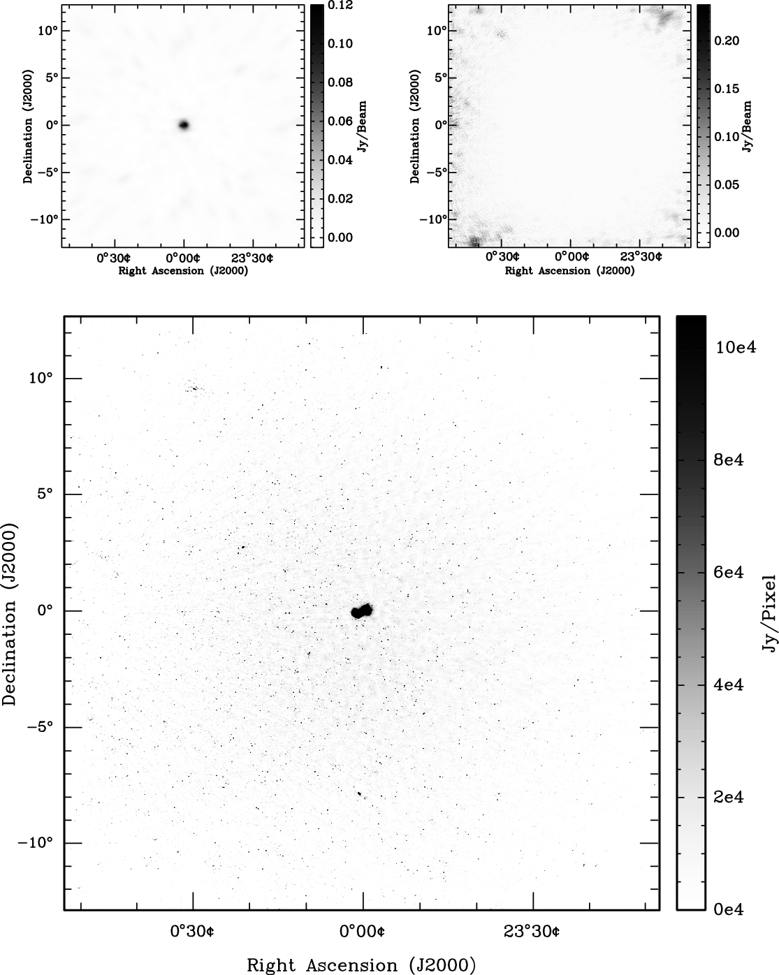
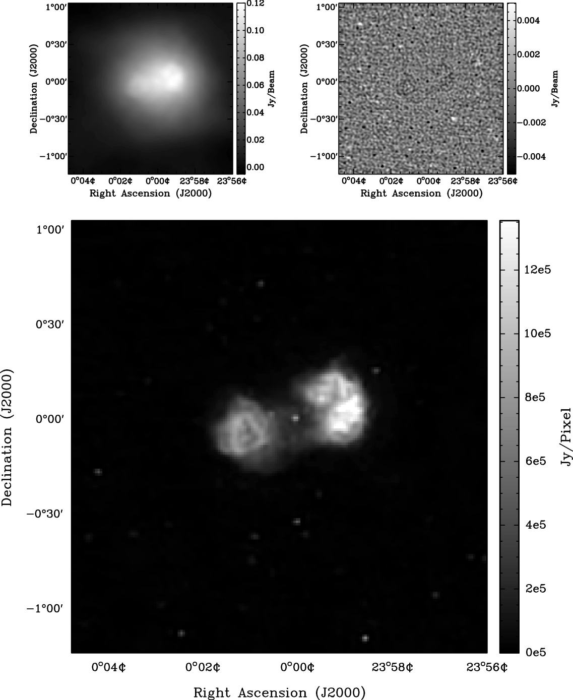
Figure 5 shows a zoom in of Figure 4, with the colour scale adjusted to show the reconstruction of Fornax A in greater detail. From the scaled residuals, it is clear that this reconstruction accurately models the extended structure of Fornax A.
Same as Figure 4 zoomed view centred on Fornax A, showing the recovered structure of the double lobed radio galaxy. The residuals have been scaled to show the details. The residuals over the zoomed region have an RMS of 1.2 mJy beam−1.
6. Improvements for the future
We discuss two classes of possible improvements: kernel interpolations and correction for non-standard DDEs.
6.1. Kernel interpolation
While we have shown that the use of k-means clustering and complex conjugation can aid in kernel construction, w-projection kernels can still be expensive in construction time due to the large number of coefficients in  ${\textsf{GC}}$
. This construction overhead can be further reduced using interpolation methods, such as bilinear interpolation between 1d w-planes, or parametric fitting. This may allow for on the fly calculation of kernels during imaging. We discuss how a radially symmetric kernel could affect such methods in the future.
${\textsf{GC}}$
. This construction overhead can be further reduced using interpolation methods, such as bilinear interpolation between 1d w-planes, or parametric fitting. This may allow for on the fly calculation of kernels during imaging. We discuss how a radially symmetric kernel could affect such methods in the future.
6.1.1. w-planes: Bilinear interpolation
The radially symmetric kernel allows fast and accurate calculation, while reducing the dimensions of the kernel. This allows for fast and accurate pre-sampling of the w-projection kernel directly in the uvw-domain, in some cases to a sufficient pre-sampling density that the error from linear interpolation is negligible compared to the aliasing error. While the mathematical basis for bilinear interpolation is discussed in detail in Paper I, here we present the implementation considerations.
First, we make it clear that a non-radially symmetric kernel would mean pre-sampling in  $(u_{\rm pix}, v_{\rm pix}, w)$
, which is a computational challenge. For
$(u_{\rm pix}, v_{\rm pix}, w)$
, which is a computational challenge. For  $N_u \times N_v$
, samples in (u, v), we would have
$N_u \times N_v$
, samples in (u, v), we would have  $N_w$
w-projection planes. This requires in total
$N_w$
w-projection planes. This requires in total  $N_uN_vN_w$
samples. The total memory required in pre-samples is
$N_uN_vN_w$
samples. The total memory required in pre-samples is  $16\times 10^{-6} \times N_uN_vN_w$
[Megabytes].
$16\times 10^{-6} \times N_uN_vN_w$
[Megabytes].
With radial symmetry, we show in Paper I that the w-projection kernel can be computed as a function of  $\left(\sqrt{u_{\rm pix}^2 + v_{\rm pix}^2}, w\right)$
. For
$\left(\sqrt{u_{\rm pix}^2 + v_{\rm pix}^2}, w\right)$
. For  $N_{uv}$
radial samples in
$N_{uv}$
radial samples in  $\sqrt{u_{\rm pix}^2 + v_{\rm pix}^2}$
, and
$\sqrt{u_{\rm pix}^2 + v_{\rm pix}^2}$
, and  $N_w$
samples in w, we have only
$N_w$
samples in w, we have only  $N_{uv}N_w$
samples. This can be thought of as pre-computing 1d w-planes, rather than 2d w-planes. Additionally, each sample only requires a 1d integral by quadrature, reducing the pre-sampling time.
$N_{uv}N_w$
samples. This can be thought of as pre-computing 1d w-planes, rather than 2d w-planes. Additionally, each sample only requires a 1d integral by quadrature, reducing the pre-sampling time.
The 1d nature of the problem suggests better scaling of pre-sampling computation time and memory, allowing extremely accurate w-projection kernels. The total memory required in pre-samples is  $16\times 10^{-6} \times N_{uv}N_w$
[Megabytes].
$16\times 10^{-6} \times N_{uv}N_w$
[Megabytes].
It is also worth noting that pre-sampling is only required for positive (u, v, w), since the complex conjugate can be used to estimate  $(u, v, -w)$
and radial symmetry can be used for negative u and v. This leads to additional memory savings in pre-sampling.
$(u, v, -w)$
and radial symmetry can be used for negative u and v. This leads to additional memory savings in pre-sampling.
Pre-sampling can be optimised for accuracy and storage by using an adaptive sampling density. The pre-samples could be stored permanently in cases where kernel construction is performed repetitively.
Bilinear interpolation is computationally cheap and could make accurate on-the-fly construction of w-projection kernels possible, which could be needed for large data such as for the Square Kilometre Array (Hollitt et al. Reference Hollitt, Johnston-Hollitt, Dehghan, Frean, Butler-Yeoman, Lorente, Shortridge and Wayth2017). In the case where storing the gridding kernels consumes more memory than the pre-sampled kernel, on-the-fly construction can be built into the  ${\textsf{GC}}$
operator, where bilinear interpolation is used on application. However, memory layout of the pre-samples would be important, since the sample look-up time could reduce the speed of the calculation considerably.
${\textsf{GC}}$
operator, where bilinear interpolation is used on application. However, memory layout of the pre-samples would be important, since the sample look-up time could reduce the speed of the calculation considerably.
6.1.2. Function fitting
Another powerful solution to improve kernel construction costs can be found from the well-known prolate spheroidal wave function (PSWF) gridding kernels, which do not have a closed-form expression.
PSWFs can be defined multiple ways, such as having optimal localisation of energy in both image and harmonic space, making them difficult to compute. They can be calculated directly through Sinc interpolation after solving a discrete eigenvalue problem, but this can be computationally expensive, or they can be calculated using a series expansion. However, this has not stopped radio astronomers using the PSWFs for decades, ever since the work of Schwab (Reference Schwab1978, Reference Schwab1980) described a custom made PSWF that has been used in CASA (McMullin et al. Reference McMullin, Waters, Schiebel, Young and Golap2007), AIPS (Greisen Reference Greisen and Heck2003), MIRIAD (Sault, Teuben, & Wright Reference Sault, Teuben, Wright, Shaw, Payne and Hayes1995), and PURIFY (Carrillo et al. Reference Carrillo, McEwen and Wiaux2014). In Schwab (Reference Schwab1978, Reference Schwab1980), a rational approximation is used to provide a stable and accurate fit to the PSWF, which has stood the test of time.
A similar approach can be used to provide an accurate fit to w-projection kernels. Put simply, it is possible to fit a radially symmetric kernel as a function of three parameters  $\left(\sqrt{u_{\rm pix}^2 + v_{\rm pix}^2}, w, \Delta u\right)$
, i.e. polynomial fitting. This has various advantages over the pre-sampling method, such as reduced storage, no pre-sampling time, and reduced look up time (which could be critical for on-the-fly application). However, stability and reliability of the fit are not guaranteed and would require further investigation.
$\left(\sqrt{u_{\rm pix}^2 + v_{\rm pix}^2}, w, \Delta u\right)$
, i.e. polynomial fitting. This has various advantages over the pre-sampling method, such as reduced storage, no pre-sampling time, and reduced look up time (which could be critical for on-the-fly application). However, stability and reliability of the fit are not guaranteed and would require further investigation.
6.2. Additional direction dependent effects
The 1d radially symmetric kernel framework can be used in conjunction with general 2d kernels that model DDEs. It is clear that the 1d w-projection kernel derivation can be extended to other analytic radially symmetric baseline-dependent effects, i.e. a function of r or  $\sqrt{u^2 +v^2}$
only. But this does not stop the inclusion of more general baseline-dependent effects, such as the spectral and polarimetric primary beams and time-dependent ionospheric models. Generating these models will require computation that may or may not be worse than the non-coplanar baseline effects, which are telescope dependent. Non-coplanar baseline effects are a special case, where the effects need to be modelled on each baseline and can be modelled in stacks of visibilities. However, in many cases, DDE models are station dependent, suggesting the computation is not as extreme as the non-coplanar case. Additionally, these effects may apply to groups of visibilities in time, frequency, and polarisation, reducing the number of effects that need to be modeled.
$\sqrt{u^2 +v^2}$
only. But this does not stop the inclusion of more general baseline-dependent effects, such as the spectral and polarimetric primary beams and time-dependent ionospheric models. Generating these models will require computation that may or may not be worse than the non-coplanar baseline effects, which are telescope dependent. Non-coplanar baseline effects are a special case, where the effects need to be modelled on each baseline and can be modelled in stacks of visibilities. However, in many cases, DDE models are station dependent, suggesting the computation is not as extreme as the non-coplanar case. Additionally, these effects may apply to groups of visibilities in time, frequency, and polarisation, reducing the number of effects that need to be modeled.
In the worst case scenario, each baseline will have different DDEs, which can be included by further convolutions (since convolution is commutative)
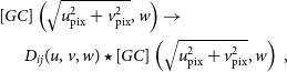 \begin{equation}\begin{split} [GC]\left(\sqrt{u_{\rm pix}^2 + v_{\rm pix}^2}, w\right) \to\quad\quad\quad\quad\quad\quad\\ D_{ij}(u, v, w) \star [GC]\left(\sqrt{u_{\rm pix}^2 + v_{\rm pix}^2}, w\right)\, , \end{split}\end{equation}
where  $D_{ij}(u, v, w)$
is a model of the DDEs in the uvw-domain between two stations ij. Typically if D(u, v, w) is band limited, the additional convolution can be performed with a discrete convolution, since
$D_{ij}(u, v, w)$
is a model of the DDEs in the uvw-domain between two stations ij. Typically if D(u, v, w) is band limited, the additional convolution can be performed with a discrete convolution, since  $[GC]\left(\sqrt{u_{\rm pix}^2 + v_{\rm pix}^2}, w, \Delta u\right)$
is also smooth. The discrete convolution has computational complexity
$[GC]\left(\sqrt{u_{\rm pix}^2 + v_{\rm pix}^2}, w, \Delta u\right)$
is also smooth. The discrete convolution has computational complexity  $\mathcal{O}(J_{GC}^2J_{D}^2)$
, where J is the width of each kernel. If D is separable in (u, v), then this can be reduced greatly to
$\mathcal{O}(J_{GC}^2J_{D}^2)$
, where J is the width of each kernel. If D is separable in (u, v), then this can be reduced greatly to  $\mathcal{O}(J_{GC}^2J_{D})$
.
$\mathcal{O}(J_{GC}^2J_{D})$
.
The computation of D(u, v, w) may require modelling in the image domain with an FFT for each baseline or it may be known analytically in (u, v, w). In the case where  $D_{ij}(u, v, w) = D_j(u, v, w)\star D_i^{\star}(u, v, w)$
is separable into station-dependent effects, it greatly reduces the modelling computation from
$D_{ij}(u, v, w) = D_j(u, v, w)\star D_i^{\star}(u, v, w)$
is separable into station-dependent effects, it greatly reduces the modelling computation from  $N_{\rm Ant}(N_{\rm Ant} - 1)/2 \to N_{\rm Ant}$
kernel constructions.
$N_{\rm Ant}(N_{\rm Ant} - 1)/2 \to N_{\rm Ant}$
kernel constructions.
The w-stacking distribution structure can be applied to model other effects, such as time-dependent primary beam and ionospheric models. Distributing the visibilities into (time) t, (frequency)  $\nu$
, and (polarisation) p DDE stacks could alleviate some of the challenges of
$\nu$
, and (polarisation) p DDE stacks could alleviate some of the challenges of  $D \star GC$
construction; this applies whenever a DDE can naturally be applied to a group of baselines. For a given DDE stack, we can apply the stack’s DDE model directly in the image domain. This can be efficiently done using recent developments in the work of van der Tol, Veenboer, & Offringa (Reference van der Tol, Veenboer and Offringa2018).
$D \star GC$
construction; this applies whenever a DDE can naturally be applied to a group of baselines. For a given DDE stack, we can apply the stack’s DDE model directly in the image domain. This can be efficiently done using recent developments in the work of van der Tol, Veenboer, & Offringa (Reference van der Tol, Veenboer and Offringa2018).
7. Conclusion
We have discussed details of the w-stacking w-projection algorithm implementation, including details of the k-means clustering, introduction of conjugate symmetry to improve the computational efficiency of the current algorithm, and possible extensions to the current algorithms and code base to further improve efficiency and accuracy of the reconstructions.
We measured the time to pre-compute and apply an implementation of the MPI w-stacking w-projection algorithm. We found that the use of conjugate symmetry greatly improves the w-stacking efficiency, which reduces the cost in w-projection kernel construction and application. It is also clear that using adaptive quadrature allows kernel construction that is independent of image size, making it efficient for large high-resolution images.
We use the MPI-distributed ADMM implementation in PURIFY to reconstruct an MWA observation of Fornax A, recovering accurate sky models of the complex source Fornax A and of point sources over the entire 25 by 25 degrees field of view. We find that we can construct w-projection kernels for 7 times the number of measurements, 2.6 times faster than the time taken in Paper I (an overall saving of approximately 18 times), using the same image size, field of view, and range of w values.
In conclusion, we suggest to modifying the implementation of the 1d radial w projection kernels for large data sets, via the use of kernel interpolation and the inclusion of non-radially symmetric DDEs. Accurate correction of wide-field and instrumental effects is critical in the era of next-generation radio interferometers and is vital to achieving science goals ranging from the detection of the Epoch of Reionisation to accurately reconstructing cosmic magnetic fields.
Acknowledgements
We thank the anonymous referee for suggestions which improved the clarity of the manuscript. We thank Dr B. McKinley for providing the calibrated MWA data of Fornax A. This work was supported by the UK Engineering and Physical Sciences Research Council (EPSRC, grants EP|M011089/1). The authors acknowledge the use of the UCL Grace High Performance Computing Facility (Grace@UCL), and associated support services, in the completion of this work. MJ-H thanks the Editors for helping me to carry the fire during the editing of this manuscript. The Dunlap Institute is funded through an endowment established by the David Dunlap family and the University of Toronto.
Facilities: MWA


