


1. Introduction
The notion of first-passage time, also called the stopping time, of a stochastic process has great significance in probability literature and as such has been studied in various contexts. For instance, an important connection between first-passage times and Green’s function for a broad class of additive skip-free processes has been established in Keilson [Reference Keilson40]. For a hyper-exponential jump diffusion process, many important probabilistic properties related to the first-passage times such as finiteness, expectation, conditional memorylessness, and conditional independence are studied in Cai [Reference Cai20], while the problem of obtaining the distributions of the first-passage times to flat boundaries for the said process has been investigated in Yin et al. [Reference Yin, Shen and Wen80]. Gitterman [Reference Gitterman29] evaluates the mean of the first-passage time, denoted as MFPT, for the anomalous diffusion, and has shown that MFPT can exhibit non-monotonic trends with the degree of departure from normal diffusion. First-passage times also have a significant role in the domain of mathematical finance (see [Reference Alili and Kyprianou2], [Reference Dong, Wang and Wu26], [Reference Kou51], [Reference Kou and Wang52], etc.).
In reliability theory, while modelling deterioration or ageing of systems, first-passage times of Markov processes arise naturally in the context of devices subject to shocks and wear during their operation. For deterioration models, the first-passage time is simply the lifetime of a unit which fails whenever a critical threshold is exceeded. While obtaining the distribution of first-passage times has received a great deal of attention in the literature (see e.g. [Reference Darling and Siegert24], [Reference Mehr and McFadden63], [Reference Siegert74–Reference Wang and Uhlenbeck77], etc.), it becomes of fundamental importance to analyse relevant conditions under which the distribution function of the first-passage time possesses various ageing properties pertaining to reliability and maintenance. First-passage times of Markov processes having PF $_r$
(Pólya frequency of order r) density are investigated in Assaf et al. [Reference Assaf and Shaked5]. Brown and Chaganty [Reference Brown and Chaganty18] investigated the IFR property of first-passage times which was further studied in Durham et al. [Reference Durham, Lynch and Padgett27]. Sufficient conditions ensuring the discrete IFRA property of first-passage times were also established in Brown and Chaganty [Reference Brown and Chaganty18], whose continuous analogues were given in Shaked and Shanthikumar [Reference Shaked and Shanthikumar72]. The NBU case has been considered by Marshall and Shaked [Reference Marshall and Shaked59, Reference Marshall and Shaked60] and also by Shanthikumar [Reference Shanthikumar73]. For an increasing Markov process, the NBUE and NWUE properties were discussed in Karasu and Özekici [Reference Karasu and Özekici35]. Subsequently, Lam [Reference Lam54] extended their work to the framework of a general Markov renewal process and further showed that under certain conditions, a more general class of stochastic processes possess the NBUE property. NBUC and DMRL classes have been studied in Pérez-Ocón and Gámiz-Pérez [Reference Pérez-Ocón and Gámiz-Pérez67]. Belzunce et al. [Reference Belzunce, Ortega and Ruiz11] have considered the problem in the context of four important classes, namely IFR(2), NBU(2) and DRL
$_r$
(Pólya frequency of order r) density are investigated in Assaf et al. [Reference Assaf and Shaked5]. Brown and Chaganty [Reference Brown and Chaganty18] investigated the IFR property of first-passage times which was further studied in Durham et al. [Reference Durham, Lynch and Padgett27]. Sufficient conditions ensuring the discrete IFRA property of first-passage times were also established in Brown and Chaganty [Reference Brown and Chaganty18], whose continuous analogues were given in Shaked and Shanthikumar [Reference Shaked and Shanthikumar72]. The NBU case has been considered by Marshall and Shaked [Reference Marshall and Shaked59, Reference Marshall and Shaked60] and also by Shanthikumar [Reference Shanthikumar73]. For an increasing Markov process, the NBUE and NWUE properties were discussed in Karasu and Özekici [Reference Karasu and Özekici35]. Subsequently, Lam [Reference Lam54] extended their work to the framework of a general Markov renewal process and further showed that under certain conditions, a more general class of stochastic processes possess the NBUE property. NBUC and DMRL classes have been studied in Pérez-Ocón and Gámiz-Pérez [Reference Pérez-Ocón and Gámiz-Pérez67]. Belzunce et al. [Reference Belzunce, Ortega and Ruiz11] have considered the problem in the context of four important classes, namely IFR(2), NBU(2) and DRL $_{Lt}$
, NBU
$_{Lt}$
, NBU $_{Lt}$
, that arise from the ‘increasing concave order’ and the ‘Laplace transform order’ respectively.
$_{Lt}$
, that arise from the ‘increasing concave order’ and the ‘Laplace transform order’ respectively.
The present article aims to extend the research along this direction to some new ageing classes that arise naturally depending on the monotonicity of certain reliability functions, namely the mean time to failure (MTTF) function, mean inactive time (MIT) function, and reversed hazard rate (RHR) function. In recent times, the literature in reliability has focused quite heavily on these functions, and the ageing classes derived from them are, namely DMTTF (IMTTF), IMIT, and DRHR. Various probabilistic aspects have been explored in [Reference Belzunce and Martínez-Riquelme8], [Reference Corujo and Valdés23], [Reference Izadi, Sharafi and Khaledi32], [Reference Izadkhah, Amini-Seresht and Balakrishnan33], [Reference Khan, Bhattacharyya and Mitra45], [Reference Khan, Bhattacharyya and Mitra46], [Reference Lu57], [Reference Parveen64–Reference Patra and Kundu66], [Reference Qiu69], [Reference Rao and Naqvi70], [Reference Yang, Zhuang and Hu79], etc., while inferential issues have been dealt with in [Reference Bhattacharyya, Khan and Mitra12–Reference Bhattacharyya, Khan and Mitra16], [Reference Defor and Zhao25], [Reference Kattumannil, Dewan and Mathew37], [Reference Kayid and Ahmad38], [Reference Khan, Bhattacharyya and Mitra43], [Reference Khan, Bhattacharyya and Mitra44], [Reference Mansourvar and Asadi58], [Reference Mathew, Alex and Kattumannil61], [Reference Mathew, Anisha and Kattumannil62]. However, the problem of obtaining appropriate conditions in the presence of which first-passage times of a Markov process possess such ageing properties remains unexplored. The present article tries to address precisely this issue. Apart from that, the authors have also analysed certain aspects of the work of Belzunce et al. [Reference Belzunce, Ortega and Ruiz11].
Let $Y=\{Y_t,\, t\geq 0\}$
be a time homogeneous Markov process with transition function
$Y=\{Y_t,\, t\geq 0\}$
be a time homogeneous Markov process with transition function $P_t$
on a countable set
$P_t$
on a countable set $E\subset [0, +\infty]$
, where
$E\subset [0, +\infty]$
, where $Y_t$
represents age or the amount of deterioration or degradation of a device at time t. It is reasonable to assume (see [Reference Belzunce, Ortega and Ruiz11] or [Reference Karasu and Özekici35]) that Y is increasing and right continuous on E. Then Y is regular and can be defined uniquely in terms of
$Y_t$
represents age or the amount of deterioration or degradation of a device at time t. It is reasonable to assume (see [Reference Belzunce, Ortega and Ruiz11] or [Reference Karasu and Özekici35]) that Y is increasing and right continuous on E. Then Y is regular and can be defined uniquely in terms of $(X,T)= \{(X_n,T_n);\;n\geq0\}$
, provided
$(X,T)= \{(X_n,T_n);\;n\geq0\}$
, provided $\lim_{n\to \infty} T_n = +\infty$
(see Çinlar [Reference Çinlar22]), where
$\lim_{n\to \infty} T_n = +\infty$
(see Çinlar [Reference Çinlar22]), where $X_n$
is the nth state visited by Y, and
$X_n$
is the nth state visited by Y, and $T_n$
is the time of its nth jump. The embedded process X is a strictly increasing Markov chain on E with an upper-triangular transition matrix Q.
$T_n$
is the time of its nth jump. The embedded process X is a strictly increasing Markov chain on E with an upper-triangular transition matrix Q.
We consider that the device fails whenever a critical threshold $j\in E$
is exceeded, and in this paper we are interested in the first-passage time defined by the random variable
$j\in E$
is exceeded, and in this paper we are interested in the first-passage time defined by the random variable
 \begin{align} S_j=\inf\{n\geq 0\mid X_n>j\},\quad j\in E\end{align}
whenever the process is confined to discrete time, and similarly by
 \begin{align} L_j=\inf\{t\geq 0\mid Y_t>j\},\quad j\in E \end{align}
for the continuous case.
The organization of the paper is as follows. In Section 2 we recapitulate some preliminaries related to certain stochastic processes, and thereafter we present a brief introduction about the ageing classes we will be working with. Section 3 confines itself to establishing appropriate conditions under which first-passage time of a discrete-time increasing Markov chain possesses the ageing properties DMTTF (IMTTF), IMIT, and DRHR. The analogous conditions for $L_j$
are next developed in Section 4. Finally, in Section 5, we discuss certain implications that can be found among these sufficient conditions. These types of implications in the context of our concerned reliability classes have also been obtained in this section. We finally add some examples to demonstrate the practical relevance of the present work.
$L_j$
are next developed in Section 4. Finally, in Section 5, we discuss certain implications that can be found among these sufficient conditions. These types of implications in the context of our concerned reliability classes have also been obtained in this section. We finally add some examples to demonstrate the practical relevance of the present work.
Throughout this paper, we will make it a practice to write ‘increasing’ and ‘decreasing’ instead of ‘non-decreasing’ and ‘non-increasing’, respectively.
2. Notations, definitions, and related discussion
In this section we recall some well-known definitions and lay the groundwork for what follows by presenting the necessary mathematical preliminaries.
For any matrix M, define the cumulative matrix $\bar M$
as
$\bar M$
as
 \begin{align*}\bar M (i,j)= \sum _{l\leq j} M(i,l),\quad i,j\in E.\end{align*}
Then, if X starts at i, the survival function of $S_j$
can be written as
$S_j$
can be written as
 \begin{align*}\mathbb{P}(S_j>n\mid X_0=i)=\mathbb{P}(X_n\leq j \mid X_0=i) \;:\!=\; \bar Q^n (i,j)\quad \text{for all}\ n\geq 0, \ i,j\in E.\end{align*}
Again, for the transition matrix Q, we have the potential matrix of X defined by
 \begin{align*}R(i,j)=\sum_{k=0}^\infty Q^k(i,j).\end{align*}
Next we have the cumulative residual potential matrix, introduced in Pérez-Ocón and Gámiz-Pérez [Reference Pérez-Ocón and Gámiz-Pérez67], defined by
 \begin{align*}R_n(i,j)=\sum_{k=n}^\infty Q^k(i,j).\end{align*}
Belzunce et al. [Reference Belzunce, Ortega and Ruiz11] added the additional notation
 \begin{align*}R_{n,m}(i,j)=\sum_{k=n}^{n+m} Q^k(i,j).\end{align*}
Before proceeding further, it is pertinent to mention that in the proof of Theorem 1(b), Belzunce et al. [Reference Belzunce, Ortega and Ruiz11] considered $R_{0,n}$
as
$R_{0,n}$
as
 \begin{align*}R_{0,n}= \sum_{k=0}^\infty Q^k-\sum_{k=n}^\infty Q^k=R-R_n=\sum_{k=0}^{n-1} Q^k,\end{align*}
whereas in the proof of Theorem 2(b), $R_{0,n}$
is taken as
$R_{0,n}$
is taken as $R_{0,n}= R-R_{n+1}$
. To avoid any confusion, in this paper we stick to the first notation, that is,
$R_{0,n}= R-R_{n+1}$
. To avoid any confusion, in this paper we stick to the first notation, that is,
 \begin{align*}R_{0,n}(i,j)= \sum_{k=0}^{n-1} Q^k(i,j).\end{align*}
For the continuous case, the survival function of $L_j$
is given by
$L_j$
is given by
 \begin{align*}\mathbb{P}(L_j>t\mid Y_0=i)=\mathbb{P}(Y_t\leq j \mid Y_0=i)=\bar P_t (i,j)\quad\text{for all}\ t \geq 0, \ i,j\in E\end{align*}
if Y starts at i. Now the analogous notations for the process Y are as follows:
-
(a) $U(i,j) = \int_0^\infty P_v (i,j)\,{\mathrm{d}} v$
, for all
$ i,j\in E$
, represents the potential matrix,
$U(i,j) = \int_0^\infty P_v (i,j)\,{\mathrm{d}} v$
, for all
$ i,j\in E$
, represents the potential matrix, -
(b)
$U_t(i,j) = \int_t^\infty P_v (i,j)\,{\mathrm{d}} v$
, for all
$ t>0$
and
$i,j\in E$
, represents the residual potential matrix, -
(c)
$U_{t,y}(i,j) = \int_{t}^{t+y} P_v (i,j)\,{\mathrm{d}} v$
, for
$t,y>0$
and all
$ i,j\in E$
.








Consider the lifetime of a device which is represented by a non-negative random variable T having a cumulative distribution function F. We now briefly discuss the ageing classes which are the focus of the present article.
The concept of mean time to failure (MTTF) function was first introduced by Barlow and Proschan [Reference Barlow and Proschan7] in the context of age-replacement policy where the replacement takes place on failure of the item or at a predetermined time t, whichever occurs first. Let $T_{[t]}$
denote the time to the first in-service failure of an equipment under an age-replacement policy with the age-replacement time t. Then the MTTF function corresponding to F (see [Reference Barlow and Proschan7]) is defined as
$T_{[t]}$
denote the time to the first in-service failure of an equipment under an age-replacement policy with the age-replacement time t. Then the MTTF function corresponding to F (see [Reference Barlow and Proschan7]) is defined as
 \begin{align*} M_F(t) \;:\!=\; \mathbb{E}[T_{[t]}] = \dfrac{\int_o^t \bar{F}(y) \,{\mathrm{d}} y}{F(t)} \quad \text{for all $ t>0$.}\end{align*}
It is a standard practice to adopt an age-replacement policy in order to prevent unexpected in-service failures, and the MTTF function has traditionally been used to assess the performance and effectiveness of maintenance policy. Two important classes of life distributions based on the MTTF function are defined below.
Definition 2.1.
F is said to belong to the decreasing (increasing) mean time to failure (DMTTF (IMTTF)) class if $M_F(t)$
is decreasing (increasing) in t.
$M_F(t)$
is decreasing (increasing) in t.
Li and Xu [Reference Li and Xu56] introduced another ageing family, namely, new better (worse) than renewal used in the reversed hazard rate order (NBRU $_{\textit{rh}}$
(NWRU
$_{\textit{rh}}$
(NWRU $_{\textit{rh}}$
)), and also highlighted its properties. However, it turns out that these classes are identical to the DMTTF and IMTTF classes respectively. Preservation under some basic reliability operations, weak convergence issues, as well as closure under convolution are well explored for these classes (see [Reference Kayid, Ahmad, Izadkhah and Abouammoh39], [Reference Knopik49], [Reference Knopik50]). Our focus is on deriving sufficient conditions which ensure that first-passage times belong to the above classes.
$_{\textit{rh}}$
)), and also highlighted its properties. However, it turns out that these classes are identical to the DMTTF and IMTTF classes respectively. Preservation under some basic reliability operations, weak convergence issues, as well as closure under convolution are well explored for these classes (see [Reference Kayid, Ahmad, Izadkhah and Abouammoh39], [Reference Knopik49], [Reference Knopik50]). Our focus is on deriving sufficient conditions which ensure that first-passage times belong to the above classes.
The position of the DMTTF (IMTTF) class in the hierarchy of ageing classes as given in Klefsjö [Reference Klefsjö48] is as follows:
 \begin{align*}\text{IFR (DFR)} \implies\text{IFRA (DFRA)} \implies \text{DMTTF (IMTTF)}\implies \text{NBUE (NWUE)}.\end{align*}
The inactive time (IT) (see Ruiz and Navarro [Reference Ruiz and Navarro71]), defined by the random time
 \begin{align*}T_{(t)}\;:\!=\; [t-T\mid T\leq t],\end{align*}
is the amount of time that has elapsed up to time $t>0$
after failure occurs. Then the mean inactive time (MIT) is defined as
$t>0$
after failure occurs. Then the mean inactive time (MIT) is defined as
 \begin{align*} m_F(t) \;:\!=\; \mathbb{E}[T_{(t)}]= \dfrac{\int_0^t F(y)\,{\mathrm{d}} y}{F(t)} \quad \text{for all $ t>0$.}\end{align*}
Due to its widespread application in diverse fields, the function is variously known as the mean waiting time (MWT) function (see [Reference Finkelstein28]) and the mean past life (MPL) function (see [Reference Goliforushani and Asadi30]). A related ageing class is defined below.
Definition 2.2.
F is said to belong to the increasing mean inactive time (IMIT) class if $m_F(t)$
is increasing in t.
$m_F(t)$
is increasing in t.
Chandra and Roy [Reference Chandra and Roy21] pointed out that it is not possible for a non-negative random variable to have a decreasing mean inactive time (DMIT). The behaviour of the excess lifetime of a renewal process with IMIT inter-arrivals is dealt with in Li and Xu [Reference Li and Xu55]. Characterizations of the IMIT class are established in [Reference Ahmad, Kayid and Pellerey1], and weak convergence issues are discussed in [Reference Khan, Bhattacharyya and Mitra46].
Similarly to the hazard rate, the reversed hazard rate (RHR) function of a random variable T is defined as
 \begin{align*}\mu_F (t)\;:\!=\; \dfrac{f(t)}{F(t)}\quad \text{for all $ t>0$,}\end{align*}
where f(t) is the probability density function of T. It was initially termed the ‘dual failure function’ by Keilson and Sumita [Reference Keilson and Sumita42] in the context of characterizing the uniform ordering under shift and scaling. The RHR function has manifold applications including estimation of the survival function in the presence of left censored data (see [Reference Andersen, Borgan, Gill and Keiding4], [Reference Kalbfleisch and Lawless34]) and the study of Fisher information arising from weighted distributions (see [Reference Iyengar, Kvam and Singh31]). In fact it is known as ‘retro-hazard’ in survival analysis. The function also induces an important ageing class, as pointed out in Block et al. [Reference Block, Savits and Singh17].
Definition 2.3.
F is said to belong to the decreasing reversed hazard rate (DRHR) class if $\mu_F(t)$
is decreasing in t.
$\mu_F(t)$
is decreasing in t.
Block et al. [Reference Block, Savits and Singh17] also demonstrate that non-negative random variables cannot have increasing reversed hazard rates. Subsequently, Chandra and Roy [Reference Chandra and Roy21] proposed a general definition for this class for which the restriction of absolute continuity is not required.
Definition 2.4. A life distribution function F is said to be DRHR if and only if F is log-concave.
Kundu et al. [Reference Kundu, Nanda and Hu53] have shown that the DRHR property of a random variable is always transmitted to the corresponding order statistics. The discrete counterpart of the above result has been proved in a recent article by Alimohammadi et al. [Reference Alimohammadi, Balakrishnan and Simon3]. The preservation properties of the DRHR class based on the generalized order statistics (GOSs) were investigated in [Reference Wang and Zhao78]. For a general counting process stopped at a random time independent of the process, Badía [Reference Badía6] has established sufficient conditions under which the process is DRHR. Conditions under which the sequential order statistics (SOS) possess the DRHR property are studied in Burkschat and Torrado [Reference Burkschat and Torrado19].
We now want to highlight the connections between the above two classes and the fundamental class IFR. This has already been nicely illustrated in Chandra and Roy [Reference Chandra and Roy21] as follows:
 \begin{align*} f \text{ is }& \text{log-concave} \, \Longrightarrow F \text{ is DRHR} \Longleftrightarrow F \text{ is log-concave} \Longrightarrow F \text{ is IMIT}\\[5pt] & \big\Downarrow \\[5pt] & F \text{ is IFR} \Longrightarrow Y= -\log_e T \text{ is DRHR.}\end{align*}
If the lifetime of a unit is modelled by a discrete random variable S with distribution function $P_k= P(S\leq k)$
and survival function
$P_k= P(S\leq k)$
and survival function $\bar P_k\;:\!=\; 1- P_k$
, then in a similar fashion we have the following discrete versions of the above definitions.
$\bar P_k\;:\!=\; 1- P_k$
, then in a similar fashion we have the following discrete versions of the above definitions.
-
(a) Li and Xu [Reference Li and Xu56]: S is said to be DMTTF (IMTTF) if
$\sum_{i=0}^{k-1}\bar P_i/P_k$
is decreasing (increasing) in
$k\in \mathbb Z^+$
. -
(b) Goliforushani and Asadi [Reference Goliforushani and Asadi30]: S is said to be IMIT if
$\sum_{i=0}^{k-1}P_i/P_k$
is increasing in
$k\in \mathbb Z^+$
. -
(c) Badía [Reference Badía6]: S is said to be DRHR if
$P_{k+s}/P_k$
is decreasing in
$k\in \mathbb Z^+$
for every
$s>0$
.


It thus becomes abundantly clear that the classes considered in the paper have an important place in reliability literature. The authors feel that obtaining sufficient conditions for first-passage times to belong to the above classes would be a significant contribution to the literature.
3. First-passage times for discrete-time Markov chains
Let $X=\{X_n,\, n\geq 0\}$
be a discrete-time increasing Markov chain with
$X=\{X_n,\, n\geq 0\}$
be a discrete-time increasing Markov chain with $\{X_0=i\}$
and transition matrix Q. Consider
$\{X_0=i\}$
and transition matrix Q. Consider $S_j$
as defined in (1.1). In this section we explore suitable sufficient conditions for which
$S_j$
as defined in (1.1). In this section we explore suitable sufficient conditions for which $S_j$
possesses the above-mentioned ageing criteria. We start out by introducing the following notations:
$S_j$
possesses the above-mentioned ageing criteria. We start out by introducing the following notations:
-
(a)
${\underset{\tilde{}}{\bar{Q}}}{}^{n}(i,j)\;:\!=\; 1-\bar{Q}^{n}(i,j)$
, -
(b)
${\underset{\tilde{}}{\bar{R}}}{}_{0,n}(i,j)\;:\!=\; \sum_{k=0}^{n-1} {\underset{\tilde{}}{\bar{Q}}}^{k}(i,j).$


Note that $\smash{{\underset{\tilde{}}{\bar{Q}}}^{n}(i,j)}$
is simply the distribution function of
$\smash{{\underset{\tilde{}}{\bar{Q}}}^{n}(i,j)}$
is simply the distribution function of $S_j$
. We call
$S_j$
. We call ${\underset{\tilde{}}{\bar{R}}}{}_{0,n}$
the complement of
${\underset{\tilde{}}{\bar{R}}}{}_{0,n}$
the complement of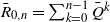 $\bar R_{0,n}= \sum_{k=0}^{n-1} \bar Q^k$
. We are now in a position to state the main results.
$\bar R_{0,n}= \sum_{k=0}^{n-1} \bar Q^k$
. We are now in a position to state the main results.
Theorem 3.1. If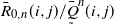 ${\bar{R}}_{0,n}(i,j)/{\underset{\tilde{}}{\bar{Q}}}^{n}(i,j)$
is decreasing in i for all
${\bar{R}}_{0,n}(i,j)/{\underset{\tilde{}}{\bar{Q}}}^{n}(i,j)$
is decreasing in i for all $ n>0$
and
$ n>0$
and $i,j \in E$
, then
$i,j \in E$
, then $S_j$
is DMTTF.
$S_j$
is DMTTF.
Proof. By definition, $S_j$
is DMTTF if, for all
$S_j$
is DMTTF if, for all $ 0<n_1\leq n_2$
,
$ 0<n_1\leq n_2$
,
 \begin{equation*} {\underset{\tilde{}}{\bar{Q}}}^{n_2}(i,j)\sum_{r=0}^{n_1-1} \bar{Q}^{r}(i,j) \geq {\underset{\tilde{}}{\bar{Q}}}^{n_1}(i,j)\sum_{r=0}^{n_2-1} \bar{Q}^{r}(i,j). \end{equation*}
Letting
 \begin{equation} \Theta = {\underset{\tilde{}}{\bar{Q}}}^{n_2}(i,j)\sum_{r=0}^{n_1-1} \bar{Q}^{r}(i,j) - {\underset{\tilde{}}{\bar{Q}}}^{n_1}(i,j)\sum_{r=0}^{n_2-1} \bar{Q}^{r}(i,j){,} \end{equation}
we only need to show that $\Theta \geq 0$
in order to prove that
$\Theta \geq 0$
in order to prove that $S_j$
is DMTTF. Now let
$S_j$
is DMTTF. Now let $n_2= n_1+m$
for some
$n_2= n_1+m$
for some $m\geq 0$
; then, using the Chapman–Kolmogorov equations, one can write
$m\geq 0$
; then, using the Chapman–Kolmogorov equations, one can write
 \begin{align*} {\underset{\tilde{}}{\bar{Q}}}^{n_2}(i,j)\sum_{r=0}^{n_1-1} \bar{Q}^{r}(i,j) &= \bigg(1 - \sum_{i\leq l\leq j} Q^{m}(i,l) \bar Q^{n_1}(l,j)\bigg) \bar{R}_{0,n_1}(i,j) \\[5pt] &= \sum_{i\leq l\leq j} Q^{m}(i,l)[1-\bar Q^{n_1}(l,j)]\bar{R}_{0,n_1}(i,j)+ \sum_{l=j+1}^\infty Q^{m}(i,l) \bar{R}_{0,n_1}(i,j) \end{align*}
and
 \begin{align*} \sum_{r=0}^{n_2-1} \bar{Q}^{r}(i,j) &= \sum_{r=0}^{n_2-1} \sum_{i\leq l\leq j} Q^{m}(i,l) \bar {Q}^{r-m}(l,j)\\[5pt] & = \sum_{i\leq l\leq j} Q^{m}(i,l) \sum_{r=0}^{n_2-1} \bar{Q}^{r-m}(l,j) \\[5pt] &= \sum_{i\leq l\leq j} Q^{m}(i,l) \sum_{r=0}^{n_1-1} \bar{Q}^{r}(l,j). \end{align*}
Then
 \begin{align*} \Theta &= \sum_{i\leq l\leq j} Q^{m}(i,l)[1-\bar Q^{n_1}(l,j)]\bar{R}_{0,n_1}(i,j)- [1- {\bar{Q}^{n_1}(i,j)}]\sum_{i\leq l\leq j} Q^{m}(i,l) \bar{R}_{0,n_1}(l,j)\\[5pt] &\quad + \sum_{l=j+1}^\infty Q^{m}(i,l) \bar{R}_{0,n_1}(i,j) \\[5pt] &\geq \sum_{i\leq l\leq j} Q^{m}(i,l)\,\bigl([1-\bar Q^{n_1}(l,j)]\bar{R}_{0,n_1}(i,j)- [1- {\bar{Q}^{n_1}(i,j)}] \bar{R}_{0,n_1}(l,j) \bigl). \end{align*}
Therefore $\Theta\geq 0$
, that is,
$\Theta\geq 0$
, that is, $S_j$
is DMTTF if, for all
$S_j$
is DMTTF if, for all $ i\leq l\leq j$
,
$ i\leq l\leq j$
,
 \begin{align*} [1-\bar Q^{n_1}(l,j)]\bar{R}_{0,n_1}(i,j)\geq [1- {\bar{Q}^{n_1}(i,j)}] \bar{R}_{0,n_1}(l,j),\end{align*}
which is equivalent to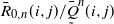 $\bar{R}_{0,n}(i,j)/{\underset{\tilde{}}{\bar{Q}}}^{n}(i,j)$
being a decreasing function of i, for all
$\bar{R}_{0,n}(i,j)/{\underset{\tilde{}}{\bar{Q}}}^{n}(i,j)$
being a decreasing function of i, for all $ n>0 $
and
$ n>0 $
and $i,j\in E$
.
$i,j\in E$
.
The mechanism of the above proof does not allow us to obtain the sufficient condition for the dual class IMTTF by just reversing the sense of monotonicity of the function in Theorem 3.1. Although it is apparent that this should be the case, the present authors are unable to either prove or disprove the fact. Instead, the sufficient condition for the corresponding dual class is framed in terms of a new function, as stated in the following theorem.
Theorem 3.2. If ${\bar{R}}_{0,n}(i,j)/{\bar{Q}}^{n}(i,j)$
is decreasing in i for all
${\bar{R}}_{0,n}(i,j)/{\bar{Q}}^{n}(i,j)$
is decreasing in i for all $ n>0$
and
$ n>0$
and $i,j \in E$
, then
$i,j \in E$
, then $S_j$
is IMTTF.
$S_j$
is IMTTF.
Proof. To prove that $S_j$
is IMTTF, we need to show that for all
$S_j$
is IMTTF, we need to show that for all $ 0<n_1\leq n_2$
,
$ 0<n_1\leq n_2$
,
 \begin{equation*} {\underset{\tilde{}}{\bar{Q}}}^{n_2}(i,j)\sum_{r=0}^{n_1-1} \bar{Q}^{r}(i,j) \leq {\underset{\tilde{}}{\bar{Q}}}^{n_1}(i,j)\sum_{r=0}^{n_2-1} \bar{Q}^{r}(i,j). \end{equation*}
Equivalently, if we consider $\Theta$
as in (3.1), then in this case it would be sufficient to prove
$\Theta$
as in (3.1), then in this case it would be sufficient to prove $\Theta\leq0$
. Now, since
$\Theta\leq0$
. Now, since $n_2=n_1+m$
for some
$n_2=n_1+m$
for some $m\geq 0$
, we have
$m\geq 0$
, we have
 \begin{align*} {\underset{\tilde{}}{\bar{Q}}}^{n_2}(i,j)\sum_{r=0}^{n_1-1} \bar{Q}^{r}(i,j) &= \sum_{r=0}^{n_1-1} \bar{Q}^{r}(i,j) - \sum_{r=0}^{n_1-1} \bar{Q}^{r}(i,j) \bar{Q}^{n_1+m}(i,j) \\[2pt] &= \sum_{r=0}^{n_1-1} \bar{Q}^{r}(i,j) - \sum_{r=0}^{n_1-1} \bar{Q}^{r}(i,j) \sum_{i\leq l\leq j}Q^m(i,l)\bar{Q}^{n_1}(l,j) \end{align*}
and
 \begin{align*} {\underset{\tilde{}}{\bar{Q}}}^{n_1}(i,j)\sum_{r=0}^{n_2-1} \bar{Q}^{r}(i,j) &= \sum_{r=0}^{n_2-1} \bar{Q}^{r}(i,j) - {\bar{Q}^{n_1}(i,j)} \sum_{r=0}^{n_1+m-1} \bar{Q}^{r}(i,j)\\[2pt] &= \sum_{r=0}^{n_2-1} \bar{Q}^{r}(i,j) - {\bar{Q}^{n_1}(i,j)} \sum_{r=0}^{n_1-1} \bar{Q}^{r+m}(i,j)\\[2pt] &= \sum_{r=0}^{n_2-1} \bar{Q}^{r}(i,j) - {\bar{Q}^{n_1}(i,j)} \sum_{r=0}^{n_1-1}\sum_{i\leq l\leq j}Q^m(i,l) \bar{Q}^{r}(l,j). \end{align*}
Then
 \begin{align*} \Theta &= \sum_{i\leq l\leq j}Q^m(i,l) \,\Biggl({\bar{Q}^{n_1}(i,j)} \sum_{r=0}^{n_1-1} \bar{Q}^{r}(l,j) - \bar{Q}^{n_1}(l,j) \sum_{r=0}^{n_1-1} \bar{Q}^{r}(i,j) \Biggl) - \sum_{r=n_1}^{n_2-1} \bar{Q}^{r}(i,j)\\[2pt] &\leq \sum_{i\leq l\leq j}Q^m(i,l)\, \Biggl({\bar{Q}^{n_1}(i,j)} \sum_{r=0}^{n_1-1} \bar{Q}^{r}(l,j) - \bar{Q}^{n_1}(l,j) \sum_{r=0}^{n_1-1} \bar{Q}^{r}(i,j) \Biggl). \end{align*}
Thus $S_j$
is IMTTF whenever
$S_j$
is IMTTF whenever
 \begin{align*}{\bar{Q}^{n_1}(i,j)} \sum_{r=0}^{n_1-1} \bar{Q}^{r}(l,j) \leq\bar{Q}^{n_1}(l,j) \sum_{r=0}^{n_1-1} \bar{Q}^{r}(i,j) \quad\text{for all $i\leq l\leq j$,}\end{align*}
which follows from the given hypothesis.
Theorem 3.3. If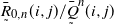 ${\underset{\tilde{}}{\bar{R}}}{}_{0,n}(i,j)/{\underset{\tilde{}}{\bar{Q}}}^{n}(i,j)$
is increasing in i, for all
${\underset{\tilde{}}{\bar{R}}}{}_{0,n}(i,j)/{\underset{\tilde{}}{\bar{Q}}}^{n}(i,j)$
is increasing in i, for all $ n>0$
and
$ n>0$
and $i,j \in E$
, then
$i,j \in E$
, then $S_j$
is IMIT.
$S_j$
is IMIT.
Proof. Define
 \begin{align*} \Theta = {\underset{\tilde{}}{\bar{Q}}}^{n_2}(i,j)\sum_{r=0}^{n_1-1}{\underset{\tilde{}}{\bar{Q}}}^{r}(i,j) - {\underset{\tilde{}}{\bar{Q}}}^{n_1}(i,j)\sum_{r=0}^{n_2-1}{\underset{\tilde{}}{\bar{Q}}}^{r}(i,j). \end{align*}
To prove $S_j$
is IMIT we only need to find out such conditions under which
$S_j$
is IMIT we only need to find out such conditions under which $\Theta\leq 0$
. Now, using the fact that
$\Theta\leq 0$
. Now, using the fact that $n_2=n_1+m$
, for some
$n_2=n_1+m$
, for some $m\geq 0$
, and then applying the Chapman–Kolmogorov equations, we have
$m\geq 0$
, and then applying the Chapman–Kolmogorov equations, we have
 \begin{align*} & {\underset{\tilde{}}{\bar{Q}}}^{n_2}(i,j)\sum_{r=0}^{n_1-1}{\underset{\tilde{}}{\bar{Q}}}^{r}(i,j)\\[2pt] &\quad = [1-\bar{Q}^{n_1+m}(i,j)]\sum_{r=0}^{n_1-1} [1-\bar{Q}^{r}(i,j)] \\[2pt] &\quad = \sum_{r=0}^{n_1-1}[1-\bar{Q}^{r}(i,j)] \Biggl(\sum_{i\leq l\leq j}Q^m(i,l)+ \sum_{j+1}^\infty Q^m(i,l) - \sum_{i\leq l\leq j}Q^m(i,l)\bar{Q}^{n_1}(l,j)\Biggr) \\[2pt] &\quad = \sum_{i\leq l\leq j}Q^m(i,l)[1-\bar{Q}^{n_1}(l,j)]\sum_{r=0}^{n_1-1}[1-\bar{Q}^{r}(i,j)]+ \sum_{j+1}^\infty Q^m(i,l)\sum_{r=0}^{n_1-1}[1-\bar{Q}^{r}(i,j)] \end{align*}
and also
 \begin{align*}& {\underset{\tilde{}}{\bar{Q}}}^{n_1}(i,j)\sum_{r=0}^{n_2-1}{\underset{\tilde{}}{\bar{Q}}}^{r}(i,j) \\[2pt]&\quad = [1- {\bar{Q}^{n_1}(i,j)}]\Biggl[(n_2-1)-\sum_{r=0}^{n_1-1}\bar{Q}^{r+m}(i,j)\Biggr] \\[2pt] &\quad = [1- {\bar{Q}^{n_1}(i,j)}]\Biggl[(n_2-1)-\sum_{r=0}^{n_1-1}\sum_{i\leq l \leq j}Q^m(i,l) \bar{Q}^{r}(l,j)\Biggr] \\[2pt] &\quad = [1- {\bar{Q}^{n_1}(i,j)}]\Biggl((n_2-1) + \sum_{i\leq l \leq j}Q^m(i,l)\sum_{r=0}^{n_1-1}[1- \bar{Q}^{r}(l,j)] -(n_1-1)\sum_{i\leq l \leq j}Q^m(i,l)\Biggr)\\[2pt] &\quad = \sum_{i\leq l \leq j}Q^m(i,l)[1- {\bar{Q}^{n_1}(i,j)}]\sum_{r=0}^{n_1-1}[1- \bar{Q}^{r}(l,j)] \\[2pt] &\quad \quad+ [1- {\bar{Q}^{n_1}(i,j)}][(n_2-1)-(n_1-1)\bar Q^m(i,j)].\end{align*}
Therefore
 \begin{align*} \Theta = \sum_{i\leq l \leq j}Q^m(i,l) \,\Biggl( [1-\bar{Q}^{n_1}(l,j)]\sum_{r=0}^{n_1-1}[1-\bar{Q}^{r}(i,j)] -[1- {\bar{Q}^{n_1}(i,j)}]\sum_{r=0}^{n_1-1}[1- \bar{Q}^{r}(l,j)]\Biggr)+ M ,\end{align*}
where
 \begin{align*} M &= \sum_{j+1}^\infty Q^m(i,l)\sum_{r=0}^{n_1-1}[1-\bar{Q}^{r}(i,j)]- [1- {\bar{Q}^{n_1}(i,j)}][(n_2-1)-(n_1-1)\bar Q^m(i,j)] \\[2pt] &= [1-\bar{Q}^{m}(i,j)]\sum_{r=0}^{n_1-1}[1-\bar{Q}^{r}(i,j)]- [1- {\bar{Q}^{n_1}(i,j)}]\bigl(m+(n_1-1)[1-\bar Q^m(i,j)]\bigr) \\[2pt] &= [1-\bar{Q}^{m}(i,j)]\,\Biggl( \sum_{r=0}^{n_1-1}[1-\bar{Q}^{r}(i,j)]- (n_1-1) [1- {\bar{Q}^{n_1}(i,j)}] \Biggr) -m [1- {\bar{Q}^{n_1}(i,j)}]\\[2pt] &= [1-\bar{Q}^{m}(i,j)] M_1-m [1- {\bar{Q}^{n_1}(i,j)}]\end{align*}
with
 \begin{align*} M_1 & = \sum_{r=0}^{n_1-1}[1-\bar{Q}^{r}(i,j)]- (n_1-1) [1- {\bar{Q}^{n_1}(i,j)}]\\[2pt]&= -\sum_{r=0}^{n_1-1}\bar{Q}^{r}(i,j)+ (n_1-1) {\bar{Q}^{n_1}(i,j)}\\[2pt]&= [-\bar{Q}^{1}(i,j)+{\bar{Q}^{n_1}(i,j)}]+[-\bar{Q}^{2}(i,j)+{\bar{Q}^{n_1}(i,j)}]+ \dots+[-\bar{Q}^{n_1-1}(i,j)+{\bar{Q}^{n_1}(i,j)}] \\[2pt]&\leq 0,\end{align*}
since the quantity ${\bar{Q}^{n_1}(i,j)}$
typically denotes the survival function of
${\bar{Q}^{n_1}(i,j)}$
typically denotes the survival function of $S_j$
for all
$S_j$
for all $n>0$
, and thus each quantity in the parentheses is non-positive. Therefore we obtain
$n>0$
, and thus each quantity in the parentheses is non-positive. Therefore we obtain
 \begin{align*} \Theta \leq \sum_{i\leq l \leq j}Q^m(i,l)\, \Biggl( [1-\bar{Q}^{n_1}(l,j)]\sum_{r=0}^{n_1-1}[1-\bar{Q}^{r}(i,j)]-[1- {\bar{Q}^{n_1}(i,j)}]\sum_{r=0}^{n_1-1}[1- \bar{Q}^{r}(l,j)]\Biggl).\end{align*}
Thus $S_j$
is IMIT whenever
$S_j$
is IMIT whenever
 \begin{align} [1-\bar{Q}^{n_1}(l,j)]\sum_{r=0}^{n_1-1}[1-\bar{Q}^{r}(i,j)]-[1- {\bar{Q}^{n_1}(i,j)}]\sum_{r=0}^{n_1-1}[1- \bar{Q}^{r}(l,j)]\leq 0 \quad \text{for all $ i\leq l \leq j$.}\end{align}
Now, substituting
 \begin{align*}\underset{\tilde{}}{{Q}}^{n}(i,j)=1-{Q}^{n}(i,j)\quad\text{and}\quad\underset{\tilde{}}{{R}}{}_{0,n}(i,j)=\sum_{r=0}^{n-1} \underset{\tilde{}}{Q}^{r}(i,j),\end{align*}
(3.2) will be equivalent to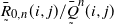 ${\underset{\tilde{}}{\bar{R}}}{}_{0,n}(i,j)/{\underset{\tilde{}}{\bar{Q}}}^{n}(i,j)$
increasing in
${\underset{\tilde{}}{\bar{R}}}{}_{0,n}(i,j)/{\underset{\tilde{}}{\bar{Q}}}^{n}(i,j)$
increasing in $i\in E$
, for all
$i\in E$
, for all $n>0$
and
$n>0$
and $j\in E$
, which is true by hypothesis.
$j\in E$
, which is true by hypothesis.
Let us recall some important definitions before going on to the next result.
Definition 3.1 (Karlin [Reference Karlin36]). Let $A,\,B\subset \mathbb R.$
A function
$A,\,B\subset \mathbb R.$
A function $K\colon A \times B\to \mathbb R^{+}$
is said to be
$K\colon A \times B\to \mathbb R^{+}$
is said to be
-
(i) totally positive of order 2 (TP
$_2$
) if
$K(x_1,y_1)K(x_2,y_2)-K(x_1,y_2)K(x_2,y_1)\geq 0$
, -
(ii) sign reverse rule of order 2 (RR
$_2$
) if
$K(x_1,y_1)K(x_2,y_2)-K(x_1,y_2)K(x_2,y_1)\leq 0$
,




for all $x_1<x_2\in A$
and
$x_1<x_2\in A$
and $y_1<y_2\in B$
.
$y_1<y_2\in B$
.
We can now proceed to the next theorem.
Theorem 3.4. If ${\underset{\tilde{}}{\bar{Q}}}^{n}(i,j)$
is
${\underset{\tilde{}}{\bar{Q}}}^{n}(i,j)$
is $RR_2$
for
$RR_2$
for $n>0$
and
$n>0$
and $i\, \,(0\leq i \leq j)$
, then
$i\, \,(0\leq i \leq j)$
, then $S_j$
is DRHR.
$S_j$
is DRHR.
Proof. Exploiting the definition of discrete DRHR, we see that $S_j$
is DRHR whenever the quantity
$S_j$
is DRHR whenever the quantity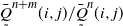 ${\underset{\tilde{}}{\bar{Q}}}^{n+m}(i,j)/{\underset{\tilde{}}{\bar{Q}}}^{n}(i,j)$
is decreasing in
${\underset{\tilde{}}{\bar{Q}}}^{n+m}(i,j)/{\underset{\tilde{}}{\bar{Q}}}^{n}(i,j)$
is decreasing in $ n\in \mathbb Z^+$
, for every
$ n\in \mathbb Z^+$
, for every $ m > 0$
and
$ m > 0$
and $ i,j\in E$
, or equivalently
$ i,j\in E$
, or equivalently
 \begin{align*} \dfrac{{\underset{\tilde{}}{\bar{Q}}}^{n_1+m}(i,j)}{{\underset{\tilde{}}{\bar{Q}}}^{n_1}(i,j)} \geq \dfrac{{\underset{\tilde{}}{\bar{Q}}}^{n_2+m}(i,j)}{{\underset{\tilde{}}{\bar{Q}}}^{n_2}(i,j)} \quad \text{for all $0<n_1\leq n_2$ and $ i,j\in E$.}\end{align*}
Now, to show that $S_j$
is DRHR, it is enough to show that
$S_j$
is DRHR, it is enough to show that
 \begin{align*}\Theta\;:\!=\; {\underset{\tilde{}}{\bar{Q}}}^{n_1+m}(i,j){\underset{\tilde{}}{\bar{Q}}}^{n_2}(i,j)-{\underset{\tilde{}}{\bar{Q}}}^{n_2+m}(i,j){\underset{\tilde{}}{\bar{Q}}}^{n_1}(i,j)\end{align*}
is non-negative. A little manipulation and an application of the Chapman–Kolmogorov equations yield
 \begin{align*} {\underset{\tilde{}}{\bar{Q}}}^{n_1+m}(i,j){\underset{\tilde{}}{\bar{Q}}}^{n_2}(i,j) &= \sum_{i\leq l \leq j} Q^m(i,l)[1-\bar{Q}^{n_1}(l,j)][1-{\bar{Q}^{n_2}(i,j)}] +\sum_{j+1}^\infty Q^m(i,l)[1-\bar{Q}^{n_2}(i,j)]\end{align*}
and
 \begin{align*} {\underset{\tilde{}}{\bar{Q}}}^{n_2+m}(i,j){\underset{\tilde{}}{\bar{Q}}}^{n_1}(i,j) = \sum_{i\leq l \leq j} Q^m(i,l)[1-\bar{Q}^{n_2}(l,j)][1-{\bar{Q}^{n_1}(i,j)}] +\sum_{j+1}^\infty Q^m(i,l)[1-\bar{Q}^{n_1}(i,j)].\end{align*}
Therefore
 \begin{align*} \Theta = \sum_{i\leq l \leq j} Q^m(i,l)\,\bigl([1-\bar{Q}^{n_1}(l,j)][1-{\bar{Q}^{n_2}(i,j)}] -[1-\bar{Q}^{n_2}(l,j)][1-{\bar{Q}^{n_1}(i,j)}] \bigl)\,+\,M,\end{align*}
where
 \begin{align*} M =\sum_{j+1}^\infty Q^m(i,l)\, \bigl([1-\bar{Q}^{n_2}(i,j)]-[1-\bar{Q}^{n_1}(i,j)]\bigl) =\sum_{j+1}^\infty Q^m(i,l)[{\bar{Q}^{n_1}(i,j)}-{\bar{Q}^{n_2}(i,j)}].\end{align*}
Since $n_2=n_1+k$
for some
$n_2=n_1+k$
for some $k\geq 0$
, we have
$k\geq 0$
, we have
 \begin{align*} M &= \sum_{j+1}^\infty Q^m(i,l)[{\bar{Q}^{n_1}(i,j)}-\bar{Q}^{n_1+k}(i,j)]\\[5pt] &= \sum_{j+1}^\infty Q^m(i,l)\Biggl[ \sum_{r\leq j}Q^{n_1}(i,r)-\sum_{i\leq r\leq j}Q^{n_1}(i,r)\bar Q^{k}(r,j)\Biggr]\\[5pt] &= \sum_{j+1}^\infty Q^m(i,l)\Biggl[ \sum_{r\leq j}Q^{n_1}(i,r)(1-\bar Q^{k}(r,j))\Biggr]\\[5pt] &\geq 0.\end{align*}
This implies
 \begin{align*}\Theta \geq \sum_{i\leq l \leq j} Q^m(i,l)\,\bigl([1-\bar{Q}^{n_1}(l,j)][1-{\bar{Q}^{n_2}(i,j)}] -[1-\bar{Q}^{n_2}(l,j)][1-{\bar{Q}^{n_1}(i,j)}] \bigr) \geq 0\end{align*}
whenever
 \begin{align*} {\underset{\tilde{}}{\bar{Q}}}^{n_1}(l,j) {\underset{\tilde{}}{\bar{Q}}}^{n_2}(i,j)-{\underset{\tilde{}}{\bar{Q}}}^{n_2}(l,j){\underset{\tilde{}}{\bar{Q}}}^{n_1}(i,j) \geq 0 , \end{align*}
where
 \begin{align*} {\underset{\tilde{}}{\bar{Q}}}^{n}(i,j)= 1-\bar Q^{n}(i,j) \geq 0 \quad \text{for all} \textit{ n and $ i,j\in E$.}\end{align*}
This is equivalent to saying that the function ${\underset{\tilde{}}{\bar{Q}}}^{n}(i,j)$
is RR
${\underset{\tilde{}}{\bar{Q}}}^{n}(i,j)$
is RR $_2$
for the variables
$_2$
for the variables $n>0$
and
$n>0$
and $i\,\,(0\leq i \leq j)$
where
$i\,\,(0\leq i \leq j)$
where $i,j \in E$
.
$i,j \in E$
.
4. First-passage times for continuous-time Markov processes
Let $Y = \{Y_t,\, t\geq 0\}$
be the regular Markov process as discussed in Section 1, with
$Y = \{Y_t,\, t\geq 0\}$
be the regular Markov process as discussed in Section 1, with $\{Y_0=i\}$
and
$\{Y_0=i\}$
and $P_t(i,j)$
being the transition function of the process. Now, as before, we introduce the following notations:
$P_t(i,j)$
being the transition function of the process. Now, as before, we introduce the following notations:
-
(a)
${\underset{\tilde{}}{ \bar P}}{}_t (i,j) \;:\!=\; 1- \bar P_t (i,j)$
, -
(b)
${\underset{\tilde{}}{\bar U}}{}_{0,t}(i,j) \;:\!=\; \int_0^{t}\underset{\tilde{}}{\bar P}{}_v (i,j)\,{\mathrm{d}} v$
for all
$ t>0$
and
$ i,j\in E$
,




where ${\underset{\tilde{}}{\bar U}}{}_{0,t}(i,j)$
represents the complement of
${\underset{\tilde{}}{\bar U}}{}_{0,t}(i,j)$
represents the complement of
 \begin{align*}\bar U_{0,t}(i,j) = \int_0^{t} \bar P_v (i,j)\,{\mathrm{d}} v\end{align*}
and ${\underset{\tilde{}}{ \bar P}}{}_t (i,j)$
is the distribution function of
${\underset{\tilde{}}{ \bar P}}{}_t (i,j)$
is the distribution function of $L_j$
. Then, under the framework of a continuous-time parameter, we have the following results.
$L_j$
. Then, under the framework of a continuous-time parameter, we have the following results.
Theorem 4.1. Let the first-passage time $L_j$
be defined as in (1.2).
$L_j$
be defined as in (1.2).
-
(i) If
$\bar U_{0,t}(i,j)/ \underset{\tilde{}}{\bar P}{}_t (i,j)$
is decreasing in
$i\in E$
for all
$ t> 0$
and
$j\in E$
, then
$L_j$
is DMTTF. -
(ii) If
$\bar U_{0,t}(i,j)/{ \bar P}_t (i,j)$
is decreasing in
$i\in E$
for all
$ t> 0$
and
$j\in E$
, then
$L_j$
is IMTTF. -
(iii) If
${\underset{\tilde{}}{\bar U}}{}_{0,t}(i,j)/ {\underset{\tilde{}}{ \bar P}}{}_t (i,j)$
is increasing in
$i\in E$
for all
$ t> 0$
and
$j\in E$
, then
$L_j$
is IMIT. -
(iv) If
$\underset{\tilde{}}{\bar P}{}_t (i,j)$
is
$RR_2$
for the variables
$t>0$
and
$i \, \,(0\leq i \leq j)$
, then
$L_j$
is DRHR.









Proof. A brief sketch of the proofs of (i), (ii), and (iv) is given. The proof of (iii) needs a little care.
(i) To prove that $L_j$
is DMTTF, we need to show
$L_j$
is DMTTF, we need to show
 \begin{align} \Phi = {\underset{\tilde{}}{ \bar P}}{}_{t_2} (i,j)\int_0^{t_1}\bar{P}_v(i,j)\, {\mathrm{d}} v- {\underset{\tilde{}}{ \bar P}}{}_{t_1} (i,j)\int_0^{t_2}\bar{P}_v(i,j)\, {\mathrm{d}} v \geq 0 \quad \text{for all $ 0<t_1\leq t_2$.}\end{align}
Applying the Chapman–Kolmogorov equations, by an argument similar to that in the discrete case, we obtain
 \begin{align*} \Phi &= \sum_{i\leq l\leq j} P_{t_2-t_1}(i,l) {\underset{\tilde{}}{ \bar P}}{}_{t_1} (l,j)\bar U_{0,t_1}(i,j) + \sum_{l=j+1}^\infty P_{t_2-t_1}(i,l) \bar U_{0,t_1}(i,j) \\ &\quad- {\underset{\tilde{}}{ \bar P}}{}_{t_1} (i,j) \sum_{i\leq l\leq j} P_{t_2-t_1}(i,l)\bar U_{0,t_1}(l,j)\\ &\geq \sum_{i\leq l\leq j} P_{t_2-t_1}(i,l)\,\bigl( {\underset{\tilde{}}{ \bar P}}{}_{t_1} (l,j)\bar U_{0,t_1}(i,j) - {\underset{\tilde{}}{ \bar P}}{}_{t_1} (i,j) \bar U_{0,t_1}(l,j)\bigr).\end{align*}
Therefore $\Phi \geq 0$
whenever
$\Phi \geq 0$
whenever
 \begin{align*} {\underset{\tilde{}}{ \bar P}}{}_{t_1} (l,j)\bar U_{0,t_1}(i,j)\geq {\underset{\tilde{}}{ \bar P}}{}_{t_1} (i,j) \bar U_{0,t_1}(l,j).\end{align*}
Thus the condition ensuring the DMTTF property of $L_j$
can be stated as
$L_j$
can be stated as
 \begin{align*} \dfrac{\bar U_{0,t}(i,j)}{{\underset{\tilde{}}{ \bar P}}{}_{t} (i,j)} \geq \dfrac{\bar U_{0,t}(l,j)}{{\underset{\tilde{}}{ \bar P}}{}_{t} (l,j)}\quad \text{for all $ i\leq l\leq j$,}\end{align*}
or equivalently $\bar U_{0,t}(i,j)/{\underset{\tilde{}}{ \bar P}}{}_{t} (i,j)$
is decreasing in i, for all
$\bar U_{0,t}(i,j)/{\underset{\tilde{}}{ \bar P}}{}_{t} (i,j)$
is decreasing in i, for all $t>0$
and
$t>0$
and $i,j\in E$
.
$i,j\in E$
.
(ii) Defining $\Phi$
as (4.1) above, we deduce that
$\Phi$
as (4.1) above, we deduce that $L_j$
is IMTTF if
$L_j$
is IMTTF if $\Phi \leq 0$
. Now an analogous manipulation to that in Theorem 3.2 yields
$\Phi \leq 0$
. Now an analogous manipulation to that in Theorem 3.2 yields
 \begin{align*} \Phi &= \int_0^{t_1}\bar P_v (i,j)\, {\mathrm{d}} v\,\Biggl(1-\sum_{i\leq l\leq j} P_{t_2-t_1}(i,l)\bar P_{t_1} (l,j)\Biggr) - \int_0^{t_2}\bar P_v (i,j)\, {\mathrm{d}} v \\[5pt] & \quad +\sum_{i\leq l\leq j} P_{t_2-t_1}(i,l)\bar P_{t_1} (i,j)\int_0^{t_1}\bar P_v (l,j)\, {\mathrm{d}} v\\[5pt] & \leq \sum_{i\leq l\leq j} P_{t_2-t_1}(i,l)\,\bigl(\bar P_{t_1} (i,j) \bar U_{0,t_1}(l,j) - \bar P_{t_1} (l,j) \bar U_{0,t_1}(i,j)\bigr).\end{align*}
Therefore $\Phi \leq 0$
for
$\Phi \leq 0$
for
 \begin{align*} \dfrac{\bar U_{0,t_1}(l,j)}{\bar P_{t_1} (l,j)}\leq \dfrac{\bar U_{0,t_1}(i,j)}{\bar P_{t_1} (i,j)} \quad \text{for all $ i\leq l\leq j$,}\end{align*}
which is true from the given hypothesis.
(iii) To show that $L_j$
possesses the IMIT property, it suffices to show that
$L_j$
possesses the IMIT property, it suffices to show that
 \begin{align*} \Phi = {\underset{\tilde{}}{ \bar P}}{}_{t_2} (i,j)\int_0^{t_1}{\underset{\tilde{}}{ \bar P}}{}_{v} (i,j)\,{\mathrm{d}} v - {\underset{\tilde{}}{ \bar P}}{}_{t_1} (i,j)\int_0^{t_2}{\underset{\tilde{}}{ \bar P}}{}_{v} (i,j)\,{\mathrm{d}} v \leq 0.\end{align*}
As before,
 \begin{align*} {\underset{\tilde{}}{ \bar P}}{}_{t_2} (i,j)\int_0^{t_1}{\underset{\tilde{}}{ \bar P}}{}_{v} (i,j)\,{\mathrm{d}} v = \sum_{i\leq l\leq j} P_{t_2-t_1}(i,l) {\underset{\tilde{}}{ \bar P}}{}_{t_1} (l,j) {\underset{\tilde{}}{\bar U}}{}_{0,t_1}(i,j) + \sum_{l=j+1}^\infty P_{t_2-t_1}(i,l) {\underset{\tilde{}}{\bar U}}{}_{0,t_1}(i,j)\end{align*}
and
 \begin{align*} & {\underset{\tilde{}}{ \bar P}}{}_{t_1} (i,j)\int_0^{t_2}{\underset{\tilde{}}{ \bar P}}{}_{v} (i,j)\,{\mathrm{d}} v \\[5pt] & \quad = \sum_{i\leq l\leq j} P_{t_2-t_1}(i,l){\underset{\tilde{}}{\bar U}}{}_{0,t_1}(l,j) {\underset{\tilde{}}{ \bar P}}{}_{t_1} (i,j) + (t_2-t_1 \bar P_{t_2-t_1}(i,j)) {\underset{\tilde{}}{ \bar P}}{}_{t_1} (i,j).\end{align*}
Thus
 \begin{align} \Phi= \sum_{i\leq l\leq j} P_{t_2-t_1}(i,l)\,\bigl( {\underset{\tilde{}}{ \bar P}}{}_{t_1} (l,j) {\underset{\tilde{}}{\bar U}}{}_{0,t_1}(i,j)-{\underset{\tilde{}}{\bar U}}{}_{0,t_1}(l,j) {\underset{\tilde{}}{ \bar P}}{}_{t_1} (i,j)\bigr)+M^{'} ,\end{align}
where
 \begin{align*} M^{'}&= \sum_{l=j+1}^\infty P_{t_2-t_1}(i,l) {\underset{\tilde{}}{\bar U}}{}_{0,t_1}(i,j)-{\underset{\tilde{}}{ \bar P}}{}_{t_1} (i,j)\, \bigl(t_2-t_1 \bar P_{t_2-t_1}(i,j)\bigr) \\[5pt] &= {\underset{\tilde{}}{ \bar P}}{}_{t_2-t_1} (i,j) {\underset{\tilde{}}{\bar U}}{}_{0,t_1}(i,j)-{\underset{\tilde{}}{ \bar P}}{}_{t_1} (i,j) \,\bigl((t_2-t_1)+t_1{\underset{\tilde{}}{ \bar P}}{}_{t_2-t_1} (i,j)\bigr)\\[5pt] &= {\underset{\tilde{}}{ \bar P}}{}_{t_2-t_1} (i,j) M^{'}_1 - (t_2-t_1) {\underset{\tilde{}}{ \bar P}}{}_{t_1} (i,j){,} \end{align*}
with
 \begin{align*} M^{'}_1= {\underset{\tilde{}}{\bar U}}{}_{0,t_1}(i,j) -t_1{\underset{\tilde{}}{ \bar P}}{}_{t_1} (i,j) = - \int_0^{t_1}\bar P_v(i,j)\,{\mathrm{d}} v +t_1\bar P_{t_1}(i,j). \end{align*}
Note that $\bar P_t(i,j)$
is the survival function of
$\bar P_t(i,j)$
is the survival function of $L_j$
and hence is a decreasing function of t. Therefore we have
$L_j$
and hence is a decreasing function of t. Therefore we have
 \begin{align*} \bar P_{t_1}(i,j) \leq \bar P_v(i,j) \quad \text{for all $ v \leq t_1$} &\implies \quad \int_0^{t_1}\bar P_{t_1}(i,j)\,{\mathrm{d}} v \leq \int_0^{t_1}\bar P_{v}(i,j)\,{\mathrm{d}} v \\[5pt] &\implies \quad t_1\bar P_{t_1}(i,j) \leq \int_0^{t_1}\bar P_v(i,j)\,{\mathrm{d}} v \\[5pt] &\implies \quad M^{'}_1 \leq 0\end{align*}
and thus $ M^{'}\leq 0$
. Now (4.2) implies
$ M^{'}\leq 0$
. Now (4.2) implies
 \begin{align*} \Phi \leq \sum_{i\leq l\leq j} P_{t_2-t_1}(i,l)\,\bigl( {\underset{\tilde{}}{ \bar P}}{}_{t_1} (l,j) {\underset{\tilde{}}{\bar U}}{}_{0,t_1}(i,j)-{\underset{\tilde{}}{\bar U}}{}_{0,t_1}(l,j) {\underset{\tilde{}}{ \bar P}}{}_{t_1} (i,j)\bigr).\end{align*}
Therefore $L_j$
enjoys the IMIT property when
$L_j$
enjoys the IMIT property when
 \begin{align*} \dfrac{ {\underset{\tilde{}}{\bar U}}{}_{0,t_1}(i,j)}{{\underset{\tilde{}}{ \bar P}}{}_{t_1} (i,j)}\leq \dfrac{{\underset{\tilde{}}{\bar U}}{}_{0,t_1}(l,j)}{{\underset{\tilde{}}{ \bar P}}{}_{t_1} (l,j)} \quad \text{for all $ i\leq l\leq j$}\end{align*}
or, in other words, ${\underset{\tilde{}}{\bar U}}{}_{0,t}(i,j)/ {\underset{\tilde{}}{ \bar P}}{}_{t} (i,j)$
is increasing in
${\underset{\tilde{}}{\bar U}}{}_{0,t}(i,j)/ {\underset{\tilde{}}{ \bar P}}{}_{t} (i,j)$
is increasing in $i\in E$
, for all
$i\in E$
, for all $ t\geq 0 $
and
$ t\geq 0 $
and $j\in E$
.
$j\in E$
.
(iv) From Definition 2.4, $L_j$
is DRHR if and only if
$L_j$
is DRHR if and only if ${\underset{\tilde{}}{ \bar P}}{}_{t} (i,j)$
, the distribution function of
${\underset{\tilde{}}{ \bar P}}{}_{t} (i,j)$
, the distribution function of $L_j$
, is log-concave, that is, for all
$L_j$
, is log-concave, that is, for all $ 0< t_1\leq t_2$
and for every
$ 0< t_1\leq t_2$
and for every $s>0$
,
$s>0$
,
 \begin{align*} \dfrac{{\underset{\tilde{}}{ \bar P}}{}_{t_1+s} (i,j)}{{\underset{\tilde{}}{ \bar P}}{}_{t_1} (i,j)} \geq \dfrac{{\underset{\tilde{}}{ \bar P}}{}_{t_2+s} (i,j)}{{\underset{\tilde{}}{ \bar P}}{}_{t_2} (i,j)}. \end{align*}
that is,
 \begin{align*} {\underset{\tilde{}}{ \bar P}}{}_{t_1+s} (i,j){\underset{\tilde{}}{ \bar P}}{}_{t_2} (i,j) - {\underset{\tilde{}}{ \bar P}}{}_{t_2+s} (i,j){\underset{\tilde{}}{ \bar P}}{}_{t_1} (i,j) \geq 0 \quad \text{for all $ 0< t_1\leq t_2 $ and $ s>0$.}\end{align*}
Defining $\Phi$
as the expression on the left-hand side of the above inequality, we have by applying the Chapman–Kolmogorov equations
$\Phi$
as the expression on the left-hand side of the above inequality, we have by applying the Chapman–Kolmogorov equations
 \begin{align*} \Phi = \sum_{i\leq l\leq j} P_{s}(i,l)\,\bigl( {\underset{\tilde{}}{ \bar P}}{}_{t_1} (l,j){\underset{\tilde{}}{ \bar P}}{}_{t_2} (i,j)-{\underset{\tilde{}}{ \bar P}}{}_{t_2} (l,j){\underset{\tilde{}}{ \bar P}}{}_{t_1} (i,j)\bigr)+M^{'} ,\end{align*}
where
 \begin{align*} M^{'}&= \sum_{ l=j+1}^\infty P_{s}(i,l)\,\bigl( {\underset{\tilde{}}{ \bar P}}{}_{t_2} (i,j)- {\underset{\tilde{}}{ \bar P}}{}_{t_1} (i,j)\bigr)\\[5pt] &= \sum_{ l=j+1}^\infty P_{s}(i,l)\,\bigl( \bar P_{t_1}(i,j)-\bar P_{t_2}(i,j)\bigr)\geq 0 \quad \text{for all $ 0< t_1\leq t_2$}\end{align*}
as $\bar P_{t}(i,j)$
, being the survival function, is decreasing in t. Hence
$\bar P_{t}(i,j)$
, being the survival function, is decreasing in t. Hence
 \begin{align*} \Phi \geq \sum_{i\leq l\leq j} P_{s}(i,l)\,\bigl( {\underset{\tilde{}}{ \bar P}}{}_{t_1} (l,j){\underset{\tilde{}}{ \bar P}}{}_{t_2} (i,j)-{\underset{\tilde{}}{ \bar P}}{}_{t_2} (l,j){\underset{\tilde{}}{ \bar P}}{}_{t_1} (i,j)\bigr).\end{align*}
Therefore $\Phi \geq 0$
, or equivalently
$\Phi \geq 0$
, or equivalently $L_j$
is DRHR if
$L_j$
is DRHR if
 \begin{align} {\underset{\tilde{}}{ \bar P}}{}_{t_1} (l,j){\underset{\tilde{}}{ \bar P}}{}_{t_2} (i,j)-{\underset{\tilde{}}{ \bar P}}{}_{t_2} (l,j){\underset{\tilde{}}{ \bar P}}{}_{t_1} (i,j) \geq 0.\end{align}
Now condition (4.3) holds due to the fact that ${\underset{\tilde{}}{ \bar P}}{}_{t} (i,j)$
is RR
${\underset{\tilde{}}{ \bar P}}{}_{t} (i,j)$
is RR $_2$
for the variables
$_2$
for the variables $t>0$
and
$t>0$
and $i\, \,(0\leq i \leq j)$
, where
$i\, \,(0\leq i \leq j)$
, where $i,j\in E$
.
$i,j\in E$
.
5. Discussion
The present work is largely concerned with obtaining appropriate conditions in the presence of which first-passage times of an increasing Markov process enjoy the DMTTF (IMTTF), IMIT, and DRHR properties. At this juncture it is pertinent to add some comments. Unlike in the case of the classical reliability classes, the functions giving rise to the ageing classes considered here have some specific forms where the distribution function figures prominently rather than the survival function. This aspect poses significant challenges in establishing relevant results concerning the first-passage times. The proofs involved for obtaining the appropriate conditions for $S_j$
and
$S_j$
and $L_j$
are neither routine nor straightforward. Also, typically the sufficient condition for the dual class can be obtained by just reversing the sense of monotonicity of the function which is present in the sufficient condition for the original class (see e.g. [Reference Belzunce, Ortega and Ruiz11]). This, however, is not the case for the DMTTF and IMTTF classes (see Theorems 3.1 and 3.2 for details). It is possible that such features appear due to the specific structure of the underlying reliability function. Again, observe that the mechanism of proof utilized in Theorem 3.4 of the present article allows us to provide a sufficient condition for
$L_j$
are neither routine nor straightforward. Also, typically the sufficient condition for the dual class can be obtained by just reversing the sense of monotonicity of the function which is present in the sufficient condition for the original class (see e.g. [Reference Belzunce, Ortega and Ruiz11]). This, however, is not the case for the DMTTF and IMTTF classes (see Theorems 3.1 and 3.2 for details). It is possible that such features appear due to the specific structure of the underlying reliability function. Again, observe that the mechanism of proof utilized in Theorem 3.4 of the present article allows us to provide a sufficient condition for $S_j$
to be IFR (DFR). Before moving on to this, we first recapitulate the following definition.
$S_j$
to be IFR (DFR). Before moving on to this, we first recapitulate the following definition.
Definition 5.1 (Barlow and Proschan [Reference Barlow and Proschan7]). A life distribution function F is said to be IFR (DFR) if and only if $\bar F$
is log-concave (log-convex).
$\bar F$
is log-concave (log-convex).
Theorem 5.1. Let the first-passage time $S_j$
of a discrete time increasing Markov chain X with transition matrix Q be defined as in Section 1.
$S_j$
of a discrete time increasing Markov chain X with transition matrix Q be defined as in Section 1.
-
(i) If
${\bar{Q}}^{n}(i,j)$
is
$RR_2$
for the variables
$n>0$
and
$i\, \,(0\leq i \leq j)$
, then
$S_j$
is IFR. -
(ii) If
${\bar{Q}}^{n}(i,j)$
is
$TP_2$
for the variables
$n>0$
and
$i\,\, (0\leq i \leq j)$
, then
$S_j$
is DFR.


Proof. (i) From Definition 5.1, $S_j$
is IFR if and only if
$S_j$
is IFR if and only if $\bar{Q}^{n}(i,j)$
is log-concave, or equivalently
$\bar{Q}^{n}(i,j)$
is log-concave, or equivalently $\bar{Q}^{n+m}(i,j)/\bar{Q}^{n}(i,j)$
is decreasing in
$\bar{Q}^{n+m}(i,j)/\bar{Q}^{n}(i,j)$
is decreasing in $ n>0$
for every
$ n>0$
for every $m>0$
and
$m>0$
and $ i,j\in E$
, that is,
$ i,j\in E$
, that is,
 \begin{align*} \dfrac{\bar{Q}^{n_1+m}(i,j)}{\bar{Q}^{n_1}(i,j)} \geq \dfrac{\bar{Q}^{n_2+m}(i,j)}{\bar{Q}^{n_2}(i,j)}\, \quad \text{for all $ 0< n_1\leq n_2$.} \end{align*}
Now let
 \begin{align*} \Theta = \bar{Q}^{n_1+m}(i,j)\bar{Q}^{n_2}(i,j)-\bar{Q}^{n_2+m}(i,j)\bar{Q}^{n_1}(i,j). \end{align*}
Applying the Chapman–Kolmogorov equations, we obtain
 \begin{align*} \Theta &= \sum_{i\leq l \leq j} Q^m(i,l)\bar{Q}^{n_1}(l,j){\bar{Q}^{n_2}(i,j)}-\sum_{i\leq l \leq j} Q^m(i,l)\bar{Q}^{n_2}(l,j){\bar{Q}^{n_1}(i,j)}\\[5pt] &=\sum_{i\leq l \leq j} Q^m(i,l)\,\bigl( \bar{Q}^{n_1}(l,j){\bar{Q}^{n_2}(i,j)}-{\bar{Q}^{n_1}(i,j)} \bar{Q}^{n_2}(l,j)\bigl).\end{align*}
Therefore $\Theta\geq 0$
, that is,
$\Theta\geq 0$
, that is, $S_j$
is IFR whenever
$S_j$
is IFR whenever $\bar{Q}^{n_1}(l,j){\bar{Q}^{n_2}(i,j)}-{\bar{Q}^{n_1}(i,j)} \bar{Q}^{n_2}(l,j)\geq 0$
. The proof now follows by noting that this inequality is immediate from the given hypothesis.
$\bar{Q}^{n_1}(l,j){\bar{Q}^{n_2}(i,j)}-{\bar{Q}^{n_1}(i,j)} \bar{Q}^{n_2}(l,j)\geq 0$
. The proof now follows by noting that this inequality is immediate from the given hypothesis.
(ii) The proof is similar and hence omitted for the sake of brevity.
Theorem 5.1 can be extended to the continuous case as well.
Theorem 5.2. Let the first-passage time $L_j$
of an increasing Markov process Y with continuous-time parameter and having transition function
$L_j$
of an increasing Markov process Y with continuous-time parameter and having transition function $P_t$
be defined as in Section 1.
$P_t$
be defined as in Section 1.
-
(i) If
${\bar{P}}_{t}(i,j)$
is
$RR_2$
for the variables
$t>0$
and
$i\, \,(0\leq i \leq j)$
, then
$L_j$
is IFR. -
(ii) If
${\bar{P}}_{t}(i,j)$
is
$TP_2$
for the variables
$t>0$
and
$i\,\, (0\leq i \leq j)$
, then
$L_j$
is DFR.


Proof. The proof is analogous to that of Theorem 5.1 and hence omitted.
It is worth noting that the hierarchical order found in the ageing classes can also be observed in the corresponding sufficient conditions. For instance, Brown and Chaganty [Reference Brown and Chaganty18] and Shaked and Shanthikumar [Reference Shaked and Shanthikumar72] have shown that the sufficient condition for the first-passage time to have the IFR property is that the transition matrix Q(i, j) is TP $_2$
, while for the IFRA case, it turns out that
$_2$
, while for the IFRA case, it turns out that $\bar Q(i,j)$
is decreasing in i for all j. By using Remark 1.1 of [Reference Keilson40], it is easy to see that Q(i, j) being TP
$\bar Q(i,j)$
is decreasing in i for all j. By using Remark 1.1 of [Reference Keilson40], it is easy to see that Q(i, j) being TP $_2$
implies that
$_2$
implies that $\bar Q(i,j)$
is decreasing in i for all j. Again, Karasu and Özekici [Reference Karasu and Özekici35] pointed out that the condition that
$\bar Q(i,j)$
is decreasing in i for all j. Again, Karasu and Özekici [Reference Karasu and Özekici35] pointed out that the condition that $\bar Q(i,j)$
is decreasing in i for all j further implies that
$\bar Q(i,j)$
is decreasing in i for all j further implies that $\bar R(i,j)$
is decreasing in i for all j, which in turn indicates that the first-passage time possesses the NBUE property. Pérez-Ocón and Gámiz-Pérez [Reference Pérez-Ocón and Gámiz-Pérez67] have established that if
$\bar R(i,j)$
is decreasing in i for all j, which in turn indicates that the first-passage time possesses the NBUE property. Pérez-Ocón and Gámiz-Pérez [Reference Pérez-Ocón and Gámiz-Pérez67] have established that if $\bar R_n(i,j)/\bar Q^n(i,j) $
is decreasing in i for all
$\bar R_n(i,j)/\bar Q^n(i,j) $
is decreasing in i for all $n>0$
and
$n>0$
and $i,j \in E$
, then
$i,j \in E$
, then $S_j$
is DMRL. Simple algebra shows that the sufficient condition obtained in Theorem 5.1 for the IFR class implies that
$S_j$
is DMRL. Simple algebra shows that the sufficient condition obtained in Theorem 5.1 for the IFR class implies that $\bar R_n(i,j)/\bar Q^n(i,j) $
is decreasing in i for all
$\bar R_n(i,j)/\bar Q^n(i,j) $
is decreasing in i for all $n>0$
and
$n>0$
and $i,j \in E$
. While establishing such connections between the conditions of IFR (as given in Brown and Chaganty [Reference Brown and Chaganty18]) and IFR(2) classes (given in [Reference Belzunce, Ortega and Ruiz11]), Belzunce et al. [Reference Belzunce, Ortega and Ruiz11] have come up with some incorrect statements. In this connection, it is also important to note that for a continuous life distribution, the classes IFR and IFR(2) are equivalent (see Theorem 3.8 in [Reference Belzunce, Hu and Khaledi10] or Proposition 2.3 in [Reference Belzunce, Gao, Hu and Pellerey9]). Although, in [Reference Belzunce, Ortega and Ruiz11], these incorrect statements arise in the context of IFR and IFR(2) ageing notions, we observe that they are fundamentally related to the TP
$i,j \in E$
. While establishing such connections between the conditions of IFR (as given in Brown and Chaganty [Reference Brown and Chaganty18]) and IFR(2) classes (given in [Reference Belzunce, Ortega and Ruiz11]), Belzunce et al. [Reference Belzunce, Ortega and Ruiz11] have come up with some incorrect statements. In this connection, it is also important to note that for a continuous life distribution, the classes IFR and IFR(2) are equivalent (see Theorem 3.8 in [Reference Belzunce, Hu and Khaledi10] or Proposition 2.3 in [Reference Belzunce, Gao, Hu and Pellerey9]). Although, in [Reference Belzunce, Ortega and Ruiz11], these incorrect statements arise in the context of IFR and IFR(2) ageing notions, we observe that they are fundamentally related to the TP $_2$
and RR
$_2$
and RR $_2$
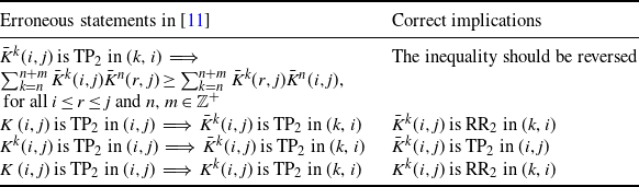
properties of a function (see Table 1). Thus the present authors find it pertinent to investigate this issue. Throughout this discussion, we adopt the notation of [Reference Belzunce, Ortega and Ruiz11] for convenience.
$_2$
properties of a function (see Table 1). Thus the present authors find it pertinent to investigate this issue. Throughout this discussion, we adopt the notation of [Reference Belzunce, Ortega and Ruiz11] for convenience.
Summary of errors in [Reference Belzunce, Ortega and Ruiz11] and their corresponding correct versions.

First of all, note that if the function $\bar K^k (i, j)$
is TP
$\bar K^k (i, j)$
is TP $_2$
in (k, i), then simple algebra yields
$_2$
in (k, i), then simple algebra yields
 \begin{align*}\sum_{k=n}^{n+m}\bar K^k (i, j)\bar K^n (r, j)\leq \sum_{k=n}^{n+m}\bar K^k (r, j)\bar K^n (i, j) \quad \text{for all $ i\leq r \leq j$ and $ n,m\in \mathbb Z^+$.}\end{align*}
Thus the statement in [Reference Belzunce, Ortega and Ruiz11, p. 255] that ‘if $\bar K^k (i, j)$
is TP
$\bar K^k (i, j)$
is TP $_2$
in (k, i), then (18) holds’, where (18) is the inequality given by ‘
$_2$
in (k, i), then (18) holds’, where (18) is the inequality given by ‘ $\sum_{k=n}^{n+m}\bar K^k (i, j)\bar K^n (r, j)\geq \sum_{k=n}^{n+m}\bar K^k (r, j)\bar K^n (i, j)$
for all
$\sum_{k=n}^{n+m}\bar K^k (i, j)\bar K^n (r, j)\geq \sum_{k=n}^{n+m}\bar K^k (r, j)\bar K^n (i, j)$
for all $i\leq r \leq j$
and
$i\leq r \leq j$
and $n,m\in\mathbb Z^+$
’, is incorrect. In fact, the inequality should be reversed. Consequently, from the condition of Theorem 1(a) in [Reference Belzunce, Ortega and Ruiz11], we have that if
$n,m\in\mathbb Z^+$
’, is incorrect. In fact, the inequality should be reversed. Consequently, from the condition of Theorem 1(a) in [Reference Belzunce, Ortega and Ruiz11], we have that if $\bar K^k (i, j)$
is TP
$\bar K^k (i, j)$
is TP $_2$
in (k, i) then
$_2$
in (k, i) then $S_j$
is DFR(2). Again, from [Reference Brown and Chaganty18],
$S_j$
is DFR(2). Again, from [Reference Brown and Chaganty18], $S_j$
is IFR whenever K (i, j) is TP
$S_j$
is IFR whenever K (i, j) is TP $_2$
in (i, j). This observation forces us to conclude that Proposition 1 of [Reference Belzunce, Ortega and Ruiz11] is incorrect. If not, it will follow that if the first-passage time
$_2$
in (i, j). This observation forces us to conclude that Proposition 1 of [Reference Belzunce, Ortega and Ruiz11] is incorrect. If not, it will follow that if the first-passage time $S_j$
is IFR then it will be DFR(2) as well. In this connection we note that in the proof of Proposition 1, Belzunce et al. [Reference Belzunce, Ortega and Ruiz11] have claimed, by referring to Corollary 3.1 of Kijima [Reference Kijima47, p. 108], that in order to show that
$S_j$
is IFR then it will be DFR(2) as well. In this connection we note that in the proof of Proposition 1, Belzunce et al. [Reference Belzunce, Ortega and Ruiz11] have claimed, by referring to Corollary 3.1 of Kijima [Reference Kijima47, p. 108], that in order to show that $\bar K^k(i,j)$
is TP
$\bar K^k(i,j)$
is TP $_2$
in (k, i), it would be enough to prove that
$_2$
in (k, i), it would be enough to prove that $ K^k(i,j)$
is TP
$ K^k(i,j)$
is TP $_2$
in (k, i). However, using Corollary 3.1 of [Reference Kijima47], it can only be shown that
$_2$
in (k, i). However, using Corollary 3.1 of [Reference Kijima47], it can only be shown that $ K^k(i,j)$
being TP
$ K^k(i,j)$
being TP $_2$
for (i, j) implies that
$_2$
for (i, j) implies that $\bar K^k(i,j)$
is TP
$\bar K^k(i,j)$
is TP $_2$
for (i, j), and not for the variables (k, i), as claimed in [Reference Belzunce, Ortega and Ruiz11]. Moreover, exploiting Theorem 2.4 in Karlin [Reference Karlin36] for the case
$_2$
for (i, j), and not for the variables (k, i), as claimed in [Reference Belzunce, Ortega and Ruiz11]. Moreover, exploiting Theorem 2.4 in Karlin [Reference Karlin36] for the case $r=2$
, one obtains that
$r=2$
, one obtains that $\bar K^k(i,j)$
is in fact RR
$\bar K^k(i,j)$
is in fact RR $_2$
in (k, i) whenever K(i, j) is TP
$_2$
in (k, i) whenever K(i, j) is TP $_2$
in (i, j). This contradicts the statement of Proposition 1 in [Reference Belzunce, Ortega and Ruiz11].
$_2$
in (i, j). This contradicts the statement of Proposition 1 in [Reference Belzunce, Ortega and Ruiz11].
Again, in the proof of Proposition 1, Belzunce et al. [Reference Belzunce, Ortega and Ruiz11] have tried to establish that $K^k(i,j)$
is TP
$K^k(i,j)$
is TP $_2$
in (k, i) whenever the condition K(i, j) is TP
$_2$
in (k, i) whenever the condition K(i, j) is TP $_2$
in (i, j) holds, by using a result pertaining to stochastic monotonicity. Belzunce et al. [Reference Belzunce, Ortega and Ruiz11] claimed that since the TP
$_2$
in (i, j) holds, by using a result pertaining to stochastic monotonicity. Belzunce et al. [Reference Belzunce, Ortega and Ruiz11] claimed that since the TP $_2$
property implies stochastic monotonicity (see [Reference Keilson and Kester41]), therefore the condition
$_2$
property implies stochastic monotonicity (see [Reference Keilson and Kester41]), therefore the condition $`K(r_2,j)\geq K(r_1,j)$
for
$`K(r_2,j)\geq K(r_1,j)$
for $ r_1\leq r_2$
’ holds due to the stochastic monotonicity property of the transition matrix K. However, this is not the case, as the notion of stochastic monotonicity deals with the row vectors of a matrix and not with some particular entries of it (see Definition 1.2 of Keilson and Kester [Reference Keilson and Kester41] for details). In this connection, note from (2.12) of Theorem 2.4 of Karlin [Reference Karlin36] that K(i, j) being TP
$ r_1\leq r_2$
’ holds due to the stochastic monotonicity property of the transition matrix K. However, this is not the case, as the notion of stochastic monotonicity deals with the row vectors of a matrix and not with some particular entries of it (see Definition 1.2 of Keilson and Kester [Reference Keilson and Kester41] for details). In this connection, note from (2.12) of Theorem 2.4 of Karlin [Reference Karlin36] that K(i, j) being TP $_2$
in (i, j) implies the condition that
$_2$
in (i, j) implies the condition that $K^k(i,j)$
is RR
$K^k(i,j)$
is RR $_2$
in (k, i).
$_2$
in (k, i).
At this juncture it seems appropriate to summarize the above discussion in a structured way. To this end, we present Table 1.
Next we highlight some connections among the sufficient conditions in the context of the reliability classes discussed in this paper. From Brown and Chaganty [Reference Brown and Chaganty18], once again note that $S_j$
is IFRA whenever
$S_j$
is IFRA whenever $\bar Q(i,j)$
is decreasing in i for all
$\bar Q(i,j)$
is decreasing in i for all $i,j \in E$
. This condition implies that for all
$i,j \in E$
. This condition implies that for all $i,j \in E$
,
$i,j \in E$
, $\bar R_{0,n}(i,j)= \sum_{k=0}^{n-1}\bar Q(i,j)$
is decreasing in i and also
$\bar R_{0,n}(i,j)= \sum_{k=0}^{n-1}\bar Q(i,j)$
is decreasing in i and also ${\underset{\tilde{}}{\bar{Q}}}^{n}(i,j)= 1- \bar{Q}^{n}(i,j)$
is increasing in i. This in turn leads to the conclusion that
${\underset{\tilde{}}{\bar{Q}}}^{n}(i,j)= 1- \bar{Q}^{n}(i,j)$
is increasing in i. This in turn leads to the conclusion that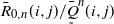 $\bar R_{0,n}(i,j)/{\underset{\tilde{}}{\bar{Q}}}^{n}(i,j)$
is decreasing in i for all
$\bar R_{0,n}(i,j)/{\underset{\tilde{}}{\bar{Q}}}^{n}(i,j)$
is decreasing in i for all $ n>0$
and
$ n>0$
and $i,j \in E$
, which is a sufficient condition for
$i,j \in E$
, which is a sufficient condition for $S_j$
to be DMTTF. On the other hand, to show that the sufficient condition for the case of the DRHR class implies that of the IMIT class, first we need to observe that the condition that
$S_j$
to be DMTTF. On the other hand, to show that the sufficient condition for the case of the DRHR class implies that of the IMIT class, first we need to observe that the condition that ${\underset{\tilde{}}{\bar{Q}}}^{n}(i,j)$
is RR
${\underset{\tilde{}}{\bar{Q}}}^{n}(i,j)$
is RR $_2$
for
$_2$
for $n>0$
and
$n>0$
and $i \, (0\leq i \leq j)$
is equivalent to
$i \, (0\leq i \leq j)$
is equivalent to
 \begin{align} \dfrac{\smash{{\underset{\tilde{}}{\bar{Q}}}^{n_1}(i,j)}_{\vphantom{1_{1_{1_.}}}}}{{\underset{\tilde{}}{\bar{Q}}}^{n_2}(i,j)}\leq \dfrac{\smash{{\underset{\tilde{}}{\bar{Q}}}^{n_1}(r,j)}_{\vphantom{1_{1_{1_.}}}}}{{\underset{\tilde{}}{\bar{Q}}}^{n_2}(r,j)}\quad \text{for all $ i\leq r \leq j $ and $ 0<n_1\leq n_2$.}\end{align}
Here our goal is to show that in the presence of condition (5.1), the function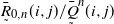 $ {\underset{\tilde{}}{\bar{R}}}{}_{0,n}(i,j)/{\underset{\tilde{}}{\bar{Q}}}^{n}(i,j)$
as given in Theorem 3.3 is increasing in i for all
$ {\underset{\tilde{}}{\bar{R}}}{}_{0,n}(i,j)/{\underset{\tilde{}}{\bar{Q}}}^{n}(i,j)$
as given in Theorem 3.3 is increasing in i for all $ n>0$
and
$ n>0$
and $i,j \in E$
. Now using (5.1) we have, for all
$i,j \in E$
. Now using (5.1) we have, for all $ i\leq r \leq j$
,
$ i\leq r \leq j$
,
 \begin{align*} \dfrac{ {\underset{\tilde{}}{\bar{R}}}{}_{0,n}(i,j)}{{\underset{\tilde{}}{\bar{Q}}}^{n}(i,j)}&= \dfrac{\sum_{k=0}^{n-1}{\underset{\tilde{}}{\bar{Q}}}^{k}(i,j)}{{\underset{\tilde{}}{\bar{Q}}}^{n}(i,j)}\\[2pt] &= \dfrac{{\underset{\tilde{}}{\bar{Q}}}^{1}(i,j)}{{\underset{\tilde{}}{\bar{Q}}}^{n}(i,j)} + \dfrac{{\underset{\tilde{}}{\bar{Q}}}^{2}(i,j)}{{\underset{\tilde{}}{\bar{Q}}}^{n}(i,j)}+\dots+ \dfrac{{\underset{\tilde{}}{\bar{Q}}}^{n-1}(i,j)}{{\underset{\tilde{}}{\bar{Q}}}^{n}(i,j)}\\[2pt] &\leq \dfrac{{\underset{\tilde{}}{\bar{Q}}}^{1}(r,j)}{{\underset{\tilde{}}{\bar{Q}}}^{n}(r,j)} + \dfrac{{\underset{\tilde{}}{\bar{Q}}}^{2}(r,j)}{{\underset{\tilde{}}{\bar{Q}}}^{n}(r,j)}+\dots+ \dfrac{{\underset{\tilde{}}{\bar{Q}}}^{n-1}(r,j)}{{\underset{\tilde{}}{\bar{Q}}}^{n}(r,j)}\\[2pt] &= \dfrac{\sum_{k=0}^{n-1}{\underset{\tilde{}}{\bar{Q}}}^{k}(r,j)}{{\underset{\tilde{}}{\bar{Q}}}^{n}(r,j)} \\[2pt] &= \dfrac{ {\underset{\tilde{}}{\bar{R}}}{}_{0,n}(r,j)}{{\underset{\tilde{}}{\bar{Q}}}^{n}(r,j)},\end{align*}
which completes the proof.
Finally, we end this section by adding some examples to strengthen the practical impact of the work. Our first example presents a Markov chain whose transition matrix satisfies the condition of Theorem 3.2 so that the first-passage time possesses the IMTTF property. It is natural that (except in the trivial case where the distribution of the first-passage time is exponential) if $S_j$
satisfies the IMTTF property then it cannot satisfy the condition for its dual class DMTTF. The following example also demonstrates this fact.
$S_j$
satisfies the IMTTF property then it cannot satisfy the condition for its dual class DMTTF. The following example also demonstrates this fact.
Example 5.1. Consider a discrete-time increasing Markov chain X with transition matrix Q given by
 \begin{align*}Q = \dfrac{1}{5}\begin{pmatrix}1\;\;\;\;\;\; & 1\;\;\;\;\;\; & 3\\[2pt] 0\;\;\;\;\;\; & 3\;\;\;\;\;\; & 2\\[2pt] 0\;\;\;\;\;\; & 0\;\;\;\;\;\; & 5\end{pmatrix}\!.\end{align*}
By induction it can be verified that
 \begin{align*}Q^n = \dfrac{1}{5^n}\begin{pmatrix}1\;\;\;\;\;\; & \frac{1}{2}(3^n-1)\;\;\;\;\;\; & 5^n- \frac{1}{2}(3^n+1)\\[2pt] 0\;\;\;\;\;\; & 3^n\;\;\;\;\;\; & 5^n-3^n\\[2pt] 0\;\;\;\;\;\; & 0\;\;\;\;\;\; & 5^n\end{pmatrix}\!.\end{align*}
It is now easy to see from Theorem 3.2 that $S_j$
is IMTTF whenever
$S_j$
is IMTTF whenever
 \begin{align} \bar{Q}^{n}(l,j) \sum_{r=0}^{n-1} \bar{Q}^{r}(i,j) \geq\bar{Q}^{n}(i,j) \sum_{r=0}^{n-1} \bar{Q}^{r}(l,j)\end{align}
holds for all ${i\leq l\leq j}$
. Taking
${i\leq l\leq j}$
. Taking $i= 1$
,
$i= 1$
, $ l=2$
,
$ l=2$
, $ j=2$
, we have from (5.2)
$ j=2$
, we have from (5.2)
 \begin{align*}\text{LHS} &= \bar{Q}^{n}(2,2) \sum_{r=0}^{n-1} \bar{Q}^{r}(1,2)\\&= \biggl(\dfrac{3}{5}\biggr)^n \sum_{r=0}^{n-1}\dfrac{1}{2\times 5^r}(3^r+1)\\&= \dfrac{1}{2}\Biggl[\biggl(\dfrac{3}{5}\biggr)^n \sum_{r=0}^{n-1}\biggl(\dfrac{3}{5}\biggr)^r+ \biggl(\dfrac{3}{5}\biggr)^n \sum_{r=0}^{n-1}\biggl(\dfrac{1}{5}\biggr)^r\Biggr]\end{align*}
and
 \begin{align*}\text{RHS}&=\bar{Q}^{n}(1,2) \sum_{r=0}^{n-1} \bar{Q}^{r}(2,2)\\&= \dfrac{1}{2\times 5^n}(3^n+1)\sum_{r=0}^{n-1}\biggl(\dfrac{3}{5}\biggr)^r\\&= \dfrac{1}{2}\Biggl[\biggl(\dfrac{3}{5}\biggr)^n \sum_{r=0}^{n-1}\biggl(\dfrac{3}{5}\biggr)^r+\biggl(\dfrac{1}{5}\biggr)^n \sum_{r=0}^{n-1}\biggl(\dfrac{3}{5}\biggr)^r\Biggr].\end{align*}
Now
 \begin{align*} 2\,\text{LHS}-2\,\text{RHS}&=\biggl(\dfrac{3}{5}\biggr)^n \sum_{r=0}^{n-1}\biggl(\dfrac{1}{5}\biggr)^r-\biggl(\dfrac{1}{5}\biggr)^n \sum_{r=0}^{n-1}\biggl(\dfrac{3}{5}\biggr)^r\\&=\dfrac{1}{5^n}\biggl[3^n\biggl(1+\dfrac{1}{5}+\dfrac{1}{5^2}+\dots+\dfrac{1}{5^{n-1}}\biggr)-\biggl(1+\dfrac{3}{5}+\dfrac{3^2}{5^2}+\dots+\dfrac{3^{n-1}}{5^{n-1}}\biggr)\biggr] \\& >0 \quad \text{for all $ n>0$,}\end{align*}
that is, the condition (5.2) is satisfied for the choice $i= 1$
,
$i= 1$
, $ l=2$
,
$ l=2$
, $ j=2.$
Note that for all other possible choices of i, l, and j, (5.2) is trivially satisfied. Thus the first-passage time
$ j=2.$
Note that for all other possible choices of i, l, and j, (5.2) is trivially satisfied. Thus the first-passage time $S_j$
possesses the IMTTF property.
$S_j$
possesses the IMTTF property.
Now we show that $S_j$
does not satisfy the condition of Theorem 3.1. The condition of Theorem 3.1 can be written as follows:
$S_j$
does not satisfy the condition of Theorem 3.1. The condition of Theorem 3.1 can be written as follows:
 \begin{align} [1- \bar{Q}^{n}(l,j)] \sum_{r=0}^{n-1} \bar{Q}^{r}(i,j) \geq [1-\bar{Q}^{n}(i,j)] \sum_{r=0}^{n-1} \bar{Q}^{r}(l,j) \quad \text{for all ${i\leq l\leq j}$.}\end{align}
Taking $i= 1$
,
$i= 1$
, $ l=2$
,
$ l=2$
, $ j=2,$
we have from (5.3)
$ j=2,$
we have from (5.3)
 \begin{align*} \text{LHS} &= [1-\bar{Q}^{n}(2,2)] \sum_{r=0}^{n-1} \bar{Q}^{r}(1,2)\\&= \biggl[1-\biggl(\dfrac{3}{5}\biggr)^n\biggr] \sum_{r=0}^{n-1}\dfrac{1}{2\times 5^r}(3^r+1) \\&= \dfrac{1}{2}\Biggl[\biggl(1-\biggl(\dfrac{3}{5}\biggr)^n\biggr) \sum_{r=0}^{n-1}\biggl(\dfrac{3}{5}\biggr)^r+ \bigg(1-\biggl(\dfrac{3}{5}\biggr)^n\bigg) \sum_{r=0}^{n-1}\biggl(\dfrac{1}{5}\biggr)^r\Biggr]\end{align*}
and
 \begin{align*} \text{RHS}&=[1-\bar{Q}^{n}(1,2)] \sum_{r=0}^{n-1} \bar{Q}^{r}(2,2)\\[2pt] &= \bigg[1-\dfrac{1}{2\times 5^n}(3^n+1)\bigg]\sum_{r=0}^{n-1}\biggl(\dfrac{3}{5}\biggr)^r\\[2pt] &= \dfrac{1}{2}\Biggl[\bigg(1-\biggl(\dfrac{3}{5}\biggr)^n\bigg) \sum_{r=0}^{n-1}\biggl(\dfrac{3}{5}\biggr)^r+\bigg(1- \biggl(\dfrac{1}{5}\biggr)^n\bigg) \sum_{r=0}^{n-1}\biggl(\dfrac{3}{5}\biggr)^r\Biggr].\end{align*}
From the above expressions it is easy to observe that $\text{LHS}<\text{RHS}$
for that particular choice of i, l, and j. This clearly violates the condition (5.3).
$\text{LHS}<\text{RHS}$
for that particular choice of i, l, and j. This clearly violates the condition (5.3).
The next example arises in a study of breast cancer. Pérez-Ocón et al. [Reference Pérez-Ocón, Ruiz-Castro and Gámiz-Pérez68] considered a continuous-time homogeneous Markov process to model the effect of treatments in survival of breast cancer. A cohort of 300 patients were given a combination of three different treatments such as chemotherapy (CT), radiotherapy (RT), and hormonal therapy (HT). In each case the impact of those treatments was categorized into three states, namely no relapse (state 1), relapse (state 2), and death (state 3). Belzunce et al. [Reference Belzunce, Ortega and Ruiz11] considered the case where all three treatments were applied to the patients, and subsequently investigated the transition matrix obtained in this scenario. Taking a cue from [Reference Belzunce, Ortega and Ruiz11], here we study the same model and show that the first-passage time of the Markov process in this case possesses the DMTTF ageing property as well.
Example 5.2. Consider the continuous-time homogeneous Markov process that models the effects of various treatments in the study of breast cancer (as discussed above) with the transition function given by
 \begin{align*} P_t= \begin{pmatrix}{\mathrm{e}}^{-(q_{12}+q_{13})t}\;\;\;\;\;\; & \dfrac{q_{12}({\mathrm{e}}^{-(q_{12}+q_{13})t}-{\mathrm{e}}^{q_{23}t})}{q_{23}-q_{12}-q_{13}}\;\;\;\;\;\; & 1-p_{11}(t)-p_{12}(t)\\[15pt] 0\;\;\;\;\;\; & {\mathrm{e}}^{-q_{13}t}\;\;\;\;\;\; & 1-{\mathrm{e}}^{-q_{13}t}\\[4pt] 0\;\;\;\;\;\; & 0\;\;\;\;\;\; & 1\end{pmatrix}\!,\end{align*}
where $q_{ij}$
is the transition intensity between the states
$q_{ij}$
is the transition intensity between the states $i,\,j$
of the Markov process whose estimated values are given by (see [Reference Belzunce, Ortega and Ruiz11])
$i,\,j$
of the Markov process whose estimated values are given by (see [Reference Belzunce, Ortega and Ruiz11])
 \begin{align*}\hat{q}_{12}= 0.0080, \quad \hat{q}_{13}=0.0024, \quad \hat{q}_{23}= 0.0408.\end{align*}
Now, to check the DMTTF property of $L_j$
, observe that condition (i) of Theorem 4.1 can be expressed as
$L_j$
, observe that condition (i) of Theorem 4.1 can be expressed as
 \begin{align} {\underset{\tilde{}}{ \bar P}}{}_{t} (l,j)\bar U_{0,t}(i,j)\geq {\underset{\tilde{}}{ \bar P}}{}_{t} (i,j) \bar U_{0,t}(l,j) \quad \text{for all $ i\leq l\leq j$.}\end{align}
Take $i= 1$
,
$i= 1$
, $l=2 $
, and
$l=2 $
, and $ j= 2$
. Writing
$ j= 2$
. Writing $\hat{q}_{12}=a,\, \hat{q}_{13}= b$
, and
$\hat{q}_{12}=a,\, \hat{q}_{13}= b$
, and $\hat{q}_{23}=c$
, from (5.4) we have
$\hat{q}_{23}=c$
, from (5.4) we have
 \begin{align*} \text{LHS}&= {\underset{\tilde{}}{ \bar P}}{}_{t} (2,2)\bar U_{0,t}(1,2)\\[2pt] &= (1-{\mathrm{e}}^{-ct})\int_0^t \bigg(\dfrac{c-b}{c-a-b}{\mathrm{e}}^{-(a+b)u}-\dfrac{a}{c-a-b}{\mathrm{e}}^{-cu}\bigg)\,{\mathrm{d}} u\\[2pt] &= (1-{\mathrm{e}}^{-ct})\biggl[\dfrac{(c-b)}{(c-a-b)(a+b)}(1-{\mathrm{e}}^{-(a+b)t}) - \dfrac{a}{c(c-a-b)}(1-{\mathrm{e}}^{-ct})\biggr]\end{align*}
and
 \begin{align*} \text{RHS}&= {\underset{\tilde{}}{ \bar P}}{}_{t} (1,2)\bar U_{0,t}(2,2)\\[2pt] &= \biggl(1-\dfrac{c-b}{c-a-b}{\mathrm{e}}^{-(a+b)t}+\dfrac{a}{c-a-b}{\mathrm{e}}^{-ct}\biggr)\int_0^t {\mathrm{e}}^{-cu}\,{\mathrm{d}} u \\[2pt] &= \biggl(1-\dfrac{c-b}{c-a-b}{\mathrm{e}}^{-(a+b)t}+\dfrac{a}{c-a-b}{\mathrm{e}}^{-ct}\biggr)\biggl(\dfrac{1}{c}-\dfrac{{\mathrm{e}}^{-cu}}{c}\biggr).\end{align*}
After some algebraic manipulation, we obtain
 \begin{align*} \text{LHS} - \text{RHS}= \dfrac{c-b}{c(a+b)}(1-{\mathrm{e}}^{-ct})(1-{\mathrm{e}}^{-(a+b)t})\geq 0, \, \quad \text{since $ c>b$.}\end{align*}
Thus the condition of (5.4) is satisfied for $i= 1$
,
$i= 1$
, $ l=2 $
, and
$ l=2 $
, and $ j= 2$
. For the other choices, the condition trivially holds. Hence
$ j= 2$
. For the other choices, the condition trivially holds. Hence $L_j$
is DMTTF.
$L_j$
is DMTTF.
We complete our work with the following example, where the conditions for the DRHR and the IMIT classes are both satisfied.
Example 5.3. Consider a continuous-time homogeneous Markov process with transition function defined by
 \begin{align*} P_t= \begin{pmatrix}\frac{1}{4}\;\;\;\;\;\; & \frac{1}{4} {\mathrm{e}}^{-4t}\;\;\;\;\;\; & \frac{3}{4} - \frac{1}{4} {\mathrm{e}}^{-4t}\\[5pt] 0\;\;\;\;\;\; & \frac{1}{4} - \frac{1}{4} {\mathrm{e}}^{-4t}\;\;\;\;\;\; & \frac{3}{4} + \frac{1}{4} {\mathrm{e}}^{-4t}\\[5pt] 0\;\;\;\;\;\; & 0\;\;\;\;\;\; & 1\end{pmatrix}\!.\end{align*}
The condition in (iv) of Theorem 4.1 is equivalent to
 \begin{align}{\underset{\tilde{}}{ \bar P}}{}_{t_1} (i,j) {\underset{\tilde{}}{ \bar P}}{}_{t_2} (l,j)\leq {\underset{\tilde{}}{ \bar P}}{}_{t_1} (l,j){\underset{\tilde{}}{ \bar P}}{}_{t_2} (i,j)\end{align}
for all $t_1< t_2$
and
$t_1< t_2$
and $i\leq l \leq j$
. Thus, for
$i\leq l \leq j$
. Thus, for $t_1< t_2$
, one only needs to verify the case where
$t_1< t_2$
, one only needs to verify the case where $i= 1$
,
$i= 1$
, $ l=2 $
, and
$ l=2 $
, and $ j= 2$
. Now
$ j= 2$
. Now
 \begin{align*} {\underset{\tilde{}}{ \bar P}}{}_{t_1} (1,2) {\underset{\tilde{}}{ \bar P}}{}_{t_2} (2,2)&= \bigg[1-\bigg(\dfrac{1}{4} + \dfrac{1}{4} {\mathrm{e}}^{-4t_1}\bigg)\bigg]\bigg[1-\bigg(\dfrac{1}{4} - \dfrac{1}{4} {\mathrm{e}}^{-4t_2}\bigg)\bigg] \\[5pt] &=\dfrac{1}{16}\bigl[9-3{\mathrm{e}}^{-4t_1}+3{\mathrm{e}}^{-4t_2}-{\mathrm{e}}^{-4(t_1+t_2)}\bigr]\end{align*}
and
 \begin{align*} {\underset{\tilde{}}{ \bar P}}{}_{t_1} (2,2) {\underset{\tilde{}}{ \bar P}}{}_{t_2} (1,2)=\dfrac{1}{16}\bigl[9+3{\mathrm{e}}^{-4t_1}-3{\mathrm{e}}^{-4t_2}-{\mathrm{e}}^{-4(t_1+t_2)}\bigr].\end{align*}
Now it is easy to see that (5.5) is satisfied and therefore $L_j$
is DRHR.
$L_j$
is DRHR.
Again, to show that $L_j$
possesses the IMIT property, note that condition (iii) of Theorem 4.1 can be expressed as
$L_j$
possesses the IMIT property, note that condition (iii) of Theorem 4.1 can be expressed as
 \begin{align} {\underset{\tilde{}}{ \bar P}}{}_{t} (l,j) {\underset{\tilde{}}{\bar U}}{}_{0,t}(i,j)\leq {\underset{\tilde{}}{\bar U}}{}_{0,t}(l,j) {\underset{\tilde{}}{ \bar P}}{}_{t} (i,j),\quad i\leq l \leq j.\end{align}
Take $i= 1$
,
$i= 1$
, $ l=2 $
, and
$ l=2 $
, and $ j= 2$
. Then
$ j= 2$
. Then
 \begin{align*} {\underset{\tilde{}}{ \bar P}}{}_{t} (2,2) {\underset{\tilde{}}{\bar U}}{}_{0,t}(1,2)&= \bigg[1-\bigg(\dfrac{1}{4}-\dfrac{1}{4}{\mathrm{e}}^{-4t}\bigg)\bigg] \int_0^t \bigg(1-\bigg(\dfrac{1}{4}+\dfrac{1}{4}{\mathrm{e}}^{-4u}\bigg)\bigg)\,{\mathrm{d}} u\\[5pt] &= \dfrac{1}{16}\bigg[9t+\dfrac{1}{2}{\mathrm{e}}^{-4t}-\dfrac{3}{4}+3t{\mathrm{e}}^{-4t}+\dfrac{1}{4}{\mathrm{e}}^{-8t}\bigg]\end{align*}
and
 \begin{align*} {\underset{\tilde{}}{ \bar P}}{}_{t} (1,2) {\underset{\tilde{}}{\bar U}}{}_{0,t}(2,2)&= \bigg[1-\bigg(\dfrac{1}{4}+\dfrac{1}{4}{\mathrm{e}}^{-4t}\bigg)\bigg] \int_0^t \bigg(1-\bigg(\dfrac{1}{4}-\dfrac{1}{4}{\mathrm{e}}^{-4u}\bigg)\bigg)\,{\mathrm{d}} u\\[5pt] &= \dfrac{1}{16}\bigg[9t-{\mathrm{e}}^{-4t}+\dfrac{3}{4}-3t{\mathrm{e}}^{-4t}+\dfrac{1}{4}{\mathrm{e}}^{-8t}\bigg].\end{align*}
Now
 \begin{align*} 16 \bigl({\underset{\tilde{}}{ \bar P}}{}_{t} (2,2) {\underset{\tilde{}}{\bar U}}{}_{0,t}(1,2)- {\underset{\tilde{}}{ \bar P}}{}_{t} (1,2) {\underset{\tilde{}}{\bar U}}{}_{0,t}(2,2)\bigr)= 6t{\mathrm{e}}^{-4t}- \dfrac{6}{4}(1-{\mathrm{e}}^{-4t})= g(t) \quad (\text{say}).\end{align*}
Note that $g(0)= 0$
and
$g(0)= 0$
and $g^{'}(t)=-24t{\mathrm{e}}^{-4t}<0$
, for all
$g^{'}(t)=-24t{\mathrm{e}}^{-4t}<0$
, for all $ t>0$
. This ensures that the condition (5.6) holds for
$ t>0$
. This ensures that the condition (5.6) holds for $i= 1$
,
$i= 1$
, $ l=2 $
, and
$ l=2 $
, and $ j= 2$
. For all the other choices of i, l, and j, the two sides of (5.6) are equal. Thus
$ j= 2$
. For all the other choices of i, l, and j, the two sides of (5.6) are equal. Thus $L_j$
possesses the IMIT property as well.
$L_j$
possesses the IMIT property as well.
Acknowledgement
The authors are indebted to the anonymous referees and the Editor for their careful reading of the manuscript. We feel that their valuable comments and constructive suggestions have led to a significant improvement in the revised manuscript.
Funding information
The first author is grateful to the Council of Scientific & Industrial Research (CSIR), Ministry of Science & Technology, Government of India for financial support.
Competing interests
There were no competing interests to declare which arose during the preparation or publication process of this article.