


1. Introduction
A large number of studies suggest that USDA forecasts are not optimal (Adjemian and Irwin, Reference Adjemian and Irwin2018; Bailey and Brorsen, Reference Bailey and Brorsen1998; Sanders and Manfredo, Reference Sanders and Manfredo2003; Isengildina et al., Reference Isengildina, Irwin and Good2006; Isengildina-Massa et al., Reference Isengildina-Massa, MacDonald and Xie2012; Xiao et al., Reference Xiao, Hart and Lence2017; Kuethe et al., Reference Kuethe, Hubbs and Sanders2018; Isengildina-Massa et al., Reference Isengildina-Massa, Karali, Kuethe and Katchova2021). Traditionally, forecast optimality is evaluated by regression-based tests of the necessary conditions of the relationships among forecasted and observed values. Like all forecasters, the USDA generates predictions that seek to minimize the costs (or disutility) experienced for differences between the observed and predicted values (forecast errors). These costs are driven by the objectives of the forecaster, including the desire for forecast accuracy, transparency, or consistency. In forecast evaluation, a forecasters’ costs are represented by a loss function, and the status quo approach assumes a priori that the USDA employs a particular loss function. However, the loss function of the USDA forecasters is unobserved. If the loss function is misspecified, regression-based tests may fail to classify a forecast as optimal even though it minimizes the forecasters’ loss function. For example, Isengildina Massa et al. (Reference Isengildina Massa, Karali and Irwin2024) suggest that the potential for USDA forecasters to minimize loss functions that deviate from the status quo have important implications for USDA forecasts, but these scenarios are not well understood.
The loss function is critical to forecast evaluation when forecasters (i) care about the differences between forecasts and observed outcomes (forecast errors) and (ii) can adjust their forecasts in a way that incorporates any costs associated with forecast errors (Elliott and Timmermann, Reference Elliott and Timmermann2008). These costs may reflect forces that are internal and external to the forecaster. Internal forces may include anticipation, hope, or fear associated with some potential outcomes (Weber, Reference Weber1994). External forces may include public reputation (Batchelor and Dua, Reference Batchelor and Dua1990; Laster et al., Reference Laster, Bennett and Geoum1999) or the desire for consistency (Batchelor, Reference Batchelor2007) or transparency (Merola and Pérez, Reference Merola and Pérez2013), as well as relationships with information providers (Francis and Philbrick, Reference Francis and Philbrick1993; Francis et al., Reference Francis, Hanna and Philbrick1997; Lim, Reference Lim2001) or forecast users (Batchelor, Reference Batchelor2007). Thus, a forecast should be evaluated based on its ability to minimize the costs experienced by the forecaster. For example, forecasters may be particularly sensitive to large deviations from observed outcomes, or alternatively, they may be more concerned about frequent small forecast errors. Similarly, forecasters may be particularly sensitive to either over- or under-predicting observed outcomes. The variation in these dimensions should determine the loss function employed in empirical forecast evaluations. A forecaster who is particularly sensitive to large forecast errors should be represented by a squared error loss function, and a forecaster who is more concerned about frequent small forecast errors should be represented by an absolute error loss function. Similarly, a forecaster who is sensitive to either over- or under-prediction should be represented by a loss function centered away from zero (Granger, Reference Granger1969). For example, Bora et al. (Reference Bora, Katchova and Kuethe2021) demonstrate that USDA production, price, and farm income forecasts are optimal under a loss function that places a larger penalty on over-prediction relative to under-prediction. Another study by Ding and Katchova (Reference Ding and Katchova2024) suggests that USDA forecasters generally realize optimality under a more relaxed unknown loss assumption.
This study proposes an alternative approach to how USDA forecasts may be evaluated. Instead of testing optimality under an assumed loss function, we posit that all USDA forecasts are produced to minimize the forecasters’ costs, and these costs can be represented by a loss function that is otherwise unobserved. Our aim, then, is to identify a mathematical representation of USDA’s unobserved loss function under which USDA forecasts could be considered optimal. Thus, we may identify candidate loss functions which may represent the unobserved costs of USDA forecasters. Specifically, we examine the degree to which ex post forecast errors conform to weak-form conditions of forecast optimality. Building on the empirical approach developed by Guler et al. (Reference Guler, Ng and Xiao2017), we estimate the traditional forecast optimality test pioneered by Mincer and Zarnowitz (Reference Mincer, Zarnowitz, Mincer and Zarnowitz1969). The Mincer and Zarnowitz method examines the conditional correlation between observed and forecasted values to test the necessary conditions of forecast optimality. Traditionally, these empirical tests are derived from coefficient restrictions on estimates produced through ordinary least squares (OLS) regression. The OLS estimates of Mincer and Zarnowitz implicitly assume that the forecasters minimize a squared error loss function centered on a mean of zero. In contrast, the Guler et al., approach employs an estimation technique in which the estimated coefficients vary across the distribution of observed outcomes conditioned on the distribution of forecasted values. Further, the loss function can consider either squared or absolute forecast errors. Instead of testing whether the forecasts are optimal under a single assumed loss function, this framework represents an alternative approach for evaluating USDA forecasts by identifying a set of potential loss functions for which USDA forecasters’ costs are minimized.
It is important to note, however, that our empirical approach is unlikely to recover a unique solution or single loss function under which a USDA forecast can be considered optimal. We may be unable to identify a unique solution because a single forecast may minimize multiple loss functions. For example, under certain distributions of observed outcomes, a forecast may be considered optimal under a mean-zero loss function with either squared or absolute errors. In addition, while our empirical approach considers a broad set of candidate loss functions, a USDA forecast still may not conform to any of these candidate loss function, even if it is optimal under other loss functions. For example, our loss functions are based on either squared or absolute errors, but some loss functions can be constructed as piecewise combinations of either quadratic or absolute error minimization (Elliott et al., Reference Elliott, Timmermann and Komunjer2005).
The USDA produces a wide range of economic forecasts, ranging from short-term production and price forecasts for a variety of commodities to aggregate farm income forecasts or long-term projections. These forecasts differ in terms of personnel, information access, and market conditions. As a result, it is likely that loss functions also vary across USDA forecasts. As an illustration, we demonstrate the degree to which the recovered loss functions vary by commodity. We apply the Guler et al. (Reference Guler, Ng and Xiao2017) approach to six quarterly animal product price forecasts from World Agricultural Supply and Demand Estimates (WASDE) from the first quarter of 1995 through the fourth quarter of 2024. The series includes forecasted and observed prices of steers, barrows and gilts, broilers, turkeys, eggs, and milk. These price forecasts were chosen for multiple reasons. First, unlike annual crop price forecasts, WASDE animal product price forecasts are produced for one- to four-quarters ahead. This format closely adheres to the macroeconomic forecasts of the Greenbok of the Federal Reserve Board of Governors, for which Guler et al. (Reference Guler, Ng and Xiao2017) developed our empirical approach. Second, compared to the annual crop price forecasts, the quarterly animal product price forecasts also provide more observations, which provide more statistical power over a shorter time period under which the forecasters loss function may change. Finally, these price forecasts have been previously evaluated by Sanders and Manfredo (Reference Sanders and Manfredo2003, Reference Sanders and Manfredo2007), who find that the degree of optimality or relationship between observed and forecasted values varies across these commodities. Thus, we explore the degree to which this variation may be attributed to the differences in the forecasters’ costs associated with each commodity. For example, we find that USDA forecasters likely experience greater costs for overpredicting the prices of steers, turkey, eggs, and milk, but we fail to reject the status quo mean-zero quadratic loss function for barrows and gilts and broilers.
This alternative approach to USDA forecast evaluation may be beneficial to both USDA forecasters and forecast users. USDA forecasters may benefit from a better understanding of their costs and how these costs guide forecasting procedures. By empirically deriving a set of candidate loss functions, forecasters can either adjust their current forecasting methods to better reflect their costs or provide guidance to forecast users about the nature of these costs. A forecast is only optimal for a specific forecast user if their loss function matches that of the forecaster (Auffhammer, Reference Auffhammer2007). Thus, a more explicit definition of USDA forecasters’ loss function benefits both forecasters and forecast users. For example, extension economists can provide a richer interpretation of USDA forecasts when these forecasts differ from their own expectations of market prices.
2. Empirical approach
The foundational test of forecast optimality was developed by Mincer and Zarnowitz (Reference Mincer, Zarnowitz, Mincer and Zarnowitz1969), which is derived from the regression equation:
 $$ A_{t+1} = \alpha + \beta F_{t+1} + \varepsilon _{t+1} $$
where A t + 1 is the actual or observed outcomes of the economic variable of interest at time t + 1, and F t + 1 is the forecast of A t + 1 conducted at time t. An optimal forecast satisfies two necessary but not sufficient conditions. First, the forecast does not consistently differ from realized values (unbiased). Second, the forecast contains all of the information available at the time it is generated (efficient). A forecast is optimal under (1) when the estimated coefficients are α = 0 (unbiased) and β = 1 (efficient). The unbiasedness and efficiency of the forecast are evaluated by testing the joint hypothesis:
 $$ H_0: \{\alpha = 0\} \cap \{\beta = 1\}. $$
Thus, a forecast is optimal if it is perfectly and positively correlated with observed outcomes, and we therefore fail to reject H 0.
Traditionally, the value of the unknown parameters α and β in (1) is estimated through OLS regression. In practice, it is therefore implicitly assumed that the forecaster minimizes the loss function:
 $$ (\hat {\alpha },\hat {\beta }) = {\rm arg\,min}_{\alpha, \beta } \sum _{t=T+1}^{T+n} (A_{t+1} - \alpha - \beta F_{t+1})^2, $$
derived from the OLS estimator, which minimizes the sum of squared errors. While researchers typically conclude that a rejection of (2) stems from nonoptimality, others argue that failure may be the result of the “joint hypothesis problem” (Fritsche et al., Reference Fritsche, Pierdzioch, Rülke and Stadtmann2015). The joint hypothesis problem argues that the rejection of optimality can stem from either a truly non-optimal forecast or a misspecified test. Within forecast evaluation, misspecification arises when the forecaster’s loss function does not conform to the assumed quadratic loss (3). As Elliott and Timmermann (Reference Elliott and Timmermann2008, p. 8) suggest, “no forecast is going to always be correct, so a specification of how costly different mistakes are is needed to guide the procedure.” The key assumption is that forecasters generate projections that minimize their costs of forecast errors, which are represented mathematically by a loss function.
A forecaster’s loss function may not conform to the assumed quadratic loss function (3) because of a variety of internal and external forces that dictate the costs associated with forecast errors. A forecaster may weight costs according to internal forces, such as optimism or pessimism, anticipation, hope, greed, or fear of specific outcomes (Batchelor, Reference Batchelor2007; Weber, Reference Weber1994). For example, in times of global political unrest, USDA forecasters may be hesitant to produce forecasts that are optimistic with respect to commodity trade, production, or prices. In addition, a forecaster may weight costs according to external forces, such as reputation or pressure from information providers and forecast users (Batchelor and Dua, Reference Batchelor and Dua1990; Batchelor, Reference Batchelor2007; Francis and Philbrick, Reference Francis and Philbrick1993; Francis et al., Reference Francis, Hanna and Philbrick1997; Laster et al., Reference Laster, Bennett and Geoum1999; Lim, Reference Lim2001). For example, farms may be adversely affected when the USDA over-predicts prices, and the related producer groups may seek to influence policymakers at the USDA or in Congress. As a result, USDA forecasters may be hesitant to provide overly optimistic price forecasts. In both of these examples, the USDA forecasters’ loss function will likely place a greater weight on over-prediction errors and favor minimizing the probability of large forecast errors. As a result, forecast optimality under (3) may be rejected even though the forecasters are minimizing their costs associated with forecast errors (Granger, Reference Granger1969).
We propose an alternative approach that seeks to identify potential loss functions under which the optimality conditions of (2) hold across the conditional distributions of observed outcomes and forecast values. Our approach builds on Guler et al. (Reference Guler, Ng and Xiao2017), who demonstrate that (1) can be estimated using quantile or expectile regression methods. We posit that the conditional quantiles or expectiles of observed outcomes and forecast values for which (2) hold reflect forecasters’ cost minimization under linear or quadratic loss, respectively. Thus, by identifying the dimensions under which optimality holds, we can better describe the costs of forecast errors experienced by USDA forecasters.
As previously mentioned, forecasters’ costs can vary across at least two important dimensions. First, forecasters may consider all forecast errors equally costly, irrespective of magnitude, as represented by a linear loss function. Alternatively, forecasters may place greater costs on larger magnitude forecast errors, as represented by a quadratic loss function. Second, forecasters may consider positive or negative forecast errors as more costly relative to the other, as represented by a loss function centered away from zero.
When a forecaster’s loss function is linear, Guler et al. (Reference Guler, Ng and Xiao2017) demonstrate that (1) can be estimated by quantile regression, a generalization of median regression (Waltrup et al., Reference Waltrup, Sobotka, Kneib and Kauermann2015). Koenker and Bassett Jr (Reference Koenker and Bassett1978) introduced quantile regression as an extension of OLS, where the conditional quantiles of the dependent variable could be modeled as a linear function of the covariates. In contrast to OLS, quantile regression estimates are the least absolute deviations minimizing solution. Koenker and Hallock (Reference Koenker and Hallock2001) emphasize that quantile regression is valuable for settings where mean regression can obscure important distributional characteristics. The corresponding loss function takes the form:
 $$ (\hat {\alpha }(\theta ), \hat {\beta }(\theta )) = {\rm arg\,min}_{\alpha, \beta } \sum _{t=T+1}^{T+n} \omega _{t,\theta } |A_{t+1} - \alpha - \beta F_{t+1}| $$
where
 $${\omega _{t,\theta }} = \left\{ {\matrix{ {1 - \theta, \;{\rm{for}}\;{A_{t + 1}} \lt \alpha - \beta {F_{t + 1}}} \cr {\theta, \;{\rm{for}}\;{A_{t + 1}} \ge \alpha - \beta {F_{t + 1}}} \cr } } \right.$$
represents the relative costs of positive and negative forecast errors with respect to the quantile of interest, represented by θ. At θ = 0.5, (4) is the median regression. If (2) holds at θ = 0.5, the estimation suggests that the forecasters may minimize a linear, symmetric median zero loss function. However, if (2) only holds at θ ≠ 0.5, the estimation suggests that the forecasters minimize a linear loss function that places a different weight on over-prediction relative to under-prediction, with θ < 0.5 placing a greater weight on over-prediction.
When a forecaster’s loss function is quadratic, Guler et al. (Reference Guler, Ng and Xiao2017) demonstrate that (1) can be estimated by expectile regression, a generalization of OLS (Waltrup et al., Reference Waltrup, Sobotka, Kneib and Kauermann2015). Powell and Newey (Reference Powell and Newey1987) developed expectile regression and noted that “expectiles may be more difficult to interpret than quantiles,” while noting useful statistical properties of expectiles. In particular, expectiles follow two important properties of coherence and elicitability, making them attractive measures of risk in banking and finance (Ziegel, Reference Ziegel2016; Nolde and Ziegel, Reference Nolde and Ziegel2017). In contrast to common measures of risk such as value at risk (VaR) and expected shortfall (ES), expectiles are capable of capturing tail risks (Bayer and Dimitriadis, Reference Bayer and Dimitriadis2020). Further, Bellini et al. (Reference Bellini, Klar, Müller and Gianin2014) show that for very heavy-tailed distributions, expectiles provide more conservative estimates than the corresponding quantiles. Given these useful properties, expectiles are proposed as alternative measures of risk (Taylor, Reference Taylor2008; Bellini and Bernardino, Reference Bellini and Bernardino2017). The corresponding loss function takes the form:
 $$ (\hat {\alpha }(\epsilon ), \hat {\beta }(\epsilon )) = {\rm arg\,min}_{\alpha, \beta } \sum _{t=T+1}^{T+n} \omega _{t,\epsilon } (A_{t+1} - \alpha - \beta F_{t+1})^2 $$
where ϵ is the expectile of interest. When ϵ = 0.5, (5) collapses to (3). If (2) holds at ϵ = 0.5, the estimation suggests that the forecasters may minimize a quadratic, symmetric mean-zero loss function. Similar to (4), if (2) only holds at ϵ ≠ 0.5, the estimation suggests that the forecasters minimize a quadratic loss function that places different weights on over-prediction relative to under-prediction, with ϵ < 0.5 placing greater weight on over-prediction.
We propose conducting a grid search across θ and ϵ to identify the values for which (2) holds. This process will identify candidate loss functions that likely minimize USDA forecasters’ costs. We can deduce the degree to which forecasters experience different costs for over- or under-prediction, under either linear or quadratic loss. Thus, instead of assuming a single default loss function a priori and testing for optimality, we assume that the forecasts are optimal and search across the dimensions of the loss function for which optimality holds.
3. Illustration
This section provides an illustration of our empirical approach to identifying the dimensions of the USDA forecasters’ loss function. As previously noted, it is possible that a single forecast minimizes multiple loss functions, and as a result, we cannot provide a unique solution. In addition, a forecast may be optimal under alternative loss functions that are not considered within the range we evaluate, such as a piecewise combination of both linear and quadratic loss fuctions (Elliott et al., Reference Elliott, Timmermann and Komunjer2005). However, given that the forecasters’ loss function is otherwise unobserved, this illustration provides a starting point for a better understanding of the costs experienced by USDA forecasters.
As previously discussed, the USDA produces a wide variety of economic forecasts which differ in terms of personnel, information access, and market conditions. Within this illustration, we examine the degree to which candidate loss functions vary across commodities. We examine six quarterly price forecasts from WASDE: steers, barrows and gilts, broilers, turkeys, eggs, and milk. Our illustration suggests that for barrows and gilts and broilers, we cannot rule out USDA’s use of the status quo mean-zero quadratic loss function, yet, for steers, eggs, and milk, our analysis suggests the use of loss functions that place a greater weight on costs associated with over-prediction relative to under-prediction. Finally, for turkeys, we fail to identify a single candidate loss function underwhich the forecasts could be considered optimal.
3.1. Data
Our illustration examines a set of price forecasts previously evaluated by Sanders and Manfredo (Reference Sanders and Manfredo2003, Reference Sanders and Manfredo2007), who demonstrate that several of these forecast errors fail to satisfy the necessary conditions for optimality assuming the status quo mean-zero quadratic loss function. The purpose of the illustration is not to show alternative tests of optimality but to use these same price series to show that the conditions of optimality may hold for alternative loss functions that deviate from the status quo mean-zero quadratic loss function.
The WASDE report, published between the 9th and the 12th of each month, summarizes the current and predicted market conditions of a number of commodities. We examine six price forecasts for animal products: steers (5-Area, Direct, Total all grades), barrows and gilts (National Base, Live equiv 51–52% lean), broilers (Wholesale, National Composite Weighted Average), turkeys (8–16 lbs, hens National), eggs (Grade A large, New York, volume buyers), and milk (prices received by farmers for all milk). The WASDE report presents animal product price forecasts in a format that is distinct from crop commodity forecasts included in the report. Each monthly report provides forecasts for the next four-quarters, including the current quarter, along with estimates for the previous four-quarters. This format closely resembles the GDP forecasts found in the Greenbook of the Federal Reserve Board of Governors, which are also produced for four-quarters-ahead and examined by Guler et al. (Reference Guler, Ng and Xiao2017) using the same empirical approach.
We follow three modeling conventions of Sanders and Manfredo (Reference Sanders and Manfredo2003, Reference Sanders and Manfredo2007). First, we examine the one-quarter-ahead price forecasts released in the first month of each quarter (i.e., January, April, July, and October). This convention avoids the problem of inconsistent OLS standard errors due to overlapping forecast horizons. Second, historically, WASDE animal product price forecasts were reported in ranges, which we examine using the midpoint of the published forecast range. Third, the quarter-ahead forecasts are examined using the log-relative price change from the corresponding quarter of the previous year. For observed price level A t and forecasted price level F t for quarter t, we define the percentage changes in observed price, a t, and forecasted price, f t as follows:
 $$\eqalign{ & {a_t} = \log \left( {{{{A_t}} \over {{A_{t - 4}}}}} \right) \cr & {f_t} = \log \left( {{{{F_t}} \over {{A_{t - 4}}}}} \right) \cr} $$
where A t − 4 is the observed price in the same quarter in the previous year. Convention suggests that this transformation helps to reduce market seasonality in observed and forecasted prices, which are common in animal products (Sanders and Manfredo, Reference Sanders and Manfredo2003, Reference Sanders and Manfredo2007). However, this transformation does not eliminate the potential for animal product price information to also have seasonal patterns. As a result, we also estimate (4) and (5) for two- and three-quarter-ahead forecasts to ensure that our results are not driven by difference in information. Our results, available in the appendix, are not sensitive to this modeling convention. Figure 1 plots the quarterly percent change in observed and forecasted prices obtained from WASDE across our observation period, the first quarter of 1995 through the second quarter of 2024.
Forecast and actual values of US animal product price forecasts from WASDE.
Source: Authors’ calculations based on USDA WASDE 1995 to 2024.

Figure 1 Long description
The image contains six line graphs showing the forecast and actual values of US animal product price forecasts from WASDE over time. The graphs are titled Barrows and Girts, Broilers, Eggs, Milk, Steers, and Turkey. Each graph has a solid line representing actual values and a dashed line representing forecast values. The x-axis represents the year, ranging from 1995 to 2025, while the y-axis represents the percentage change. The graphs illustrate the fluctuations in price changes over the years, with varying degrees of accuracy between the forecast and actual values. The data points show significant variability, with some years experiencing large deviations between the forecast and actual values. The trends and patterns in each graph provide insights into the performance of USDA forecasts over time. All values are approximated.
3.2. Results
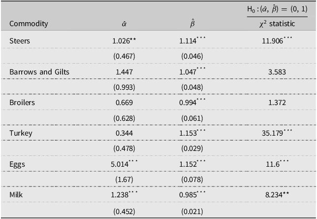
Table 1 presents the OLS estimates of the Mincer–Zarnowitz test (1) for six USDA animal product price forecasts. The final column of Table 1 reports the χ 2 value of the optimality restriction (2). As a reminder, the χ 2 test when (1) is estimated using OLS implicitly assumes that the forecasters are minimizing a mean squared error loss function centered at zero. We fail to reject (2) for barrows and gilts and broilers. Thus, for these price series, we can not rule out USDA forecasters’ use of the status quo mean-zero quadratic loss function. However, the χ 2 test is rejected at a 1% significance level for steers, turkey, and eggs, and at a 5% significance level for milk. The rejection of (2) suggests that either (i) these animal product price forecasts are not optimal or (ii) the USDA forecasters use a loss function that differs from the assumed mean-zero quadratic form.
OLS estimates of Mincer–Zarnowitz regression

Table 1 Long description
The table presents OLS estimates of the MincerZarnowitz regression for six USDA animal product price forecasts. It includes columns for commodity, alpha, beta, and chi-square statistic. The commodities listed are steers, barrows and gilts, broilers, turkey, eggs, and milk. Each row provides the estimated values for alpha and beta, along with their standard errors in parentheses, and the chi-square statistic for the optimality restriction. Notable values include steers with a chi-square statistic of 11.906, turkey with 35.179, and milk with 8.234, indicating significant results at various levels.
a Heteroskedasticity and autocorrelation consistent (HAC) standard errors are in parentheses. Significance levels: *** p < 0.01, ** p < 0.05, * p < 0.1.
Source: Authors’ calculations are based on USDA WASDE 1995 to 2024.
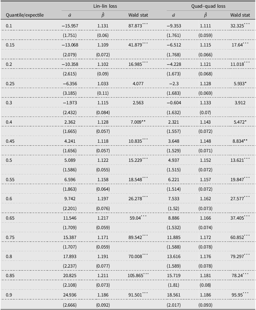
For these four cases, we also estimate (1) using quantile (4) or expectile (5) regression. To illustrate this process, Figure 4 plots the quantile regression estimates of α̂ and β̂ from both (1) and (4). Thus, the figure shows the relevant range of α̂ and β̂ for which the optimality conditions hold under linear loss. In addition, Table 2 reports the estimated coefficients and χ 2 test when (1) is estimated using quantile (4) or expectile (5) regression for eggs.Footnote 1 As a reminder, quantile regression estimation assumes that the forecasters are minimizing a linear loss function, and expectile regression estimation assumes that the forecasters are minimizing a quadratic loss function. For conditional quantiles or expectiles where (2) holds, the forecast is optimal, which may not be centered at zero. The quantile regression estimates suggest that optimality holds for θ = 0.25, 0.3. Thus, under linear loss, the results suggest that USDA forecasters minimize a loss function that places a greater weight on over-prediction errors relative to under-prediction. The expectile regression estimates suggest that optimality holds for ϵ = 0.25, 0.3, 0.35. Thus, under quadratic loss, the results also suggest that USDA forecasters may minimize a loss function that places a greater weight on over-prediction errors relative to under-prediction. Figure 2 also plots the estimated χ 2 and p-values for the optimality test at finer granularity of θ and ϵ. The figures suggest that optimality holds for conditional quantiles 0.25 − 0.40 and conditional expectiles 0.25 − 0.41.
Comparison of ordinary least squares (OLS) and quantile regression (QR) intercept and coefficient estimates. Note: The horizontal red lines represent OLS estimates with 95% confidence intervals, while the black dots and gray area represent quantile regression estimates and their 95% confidence intervals. Bootstrap Standard Errors were used to construct the confidence intervals. X-axis represent the quantile level.
Source: Authors’ calculations based on USDA WASDE 1995 to 2024.

Figure 4 Long description
The image contains eight line graphs comparing ordinary least squares (OLS) and quantile regression (QR) intercept and coefficient estimates for egg, milk, steer, and turkey prices. Each pair of graphs represents one type of price data. The horizontal red lines represent OLS estimates with 95% confidence intervals, while the black dots and gray areas represent quantile regression estimates and their 95% confidence intervals. The x-axis represents the quantile level, ranging from 0.2 to 0.8. The y-axis varies depending on the graph, showing different scales for intercept and coefficient estimates. The graphs illustrate how the estimates change across different quantile levels. The intercept estimates for egg, milk, steer, and turkey prices show an increasing trend as the quantile level increases. The coefficient estimates for these prices remain relatively stable across the quantile levels. All values are approximated.
Quantile and expectile estimates of Mincer–Zarnowitz regression for egg prices

Table 2 Long description
The table presents quantile and expectile estimates of Mincer-Zarnowitz regression for egg prices, comparing linear and quadratic loss functions. It includes columns for quantile/expectile, alpha, beta, and Wald statistics for both loss types. The table has 15 rows, each representing different quantiles or expectiles, with corresponding alpha and beta estimates and their Wald statistics. Notable trends include significant Wald statistics at various quantiles, indicating the optimality conditions under different loss functions. The estimates suggest that USDA forecasters may place a greater weight on over-prediction errors relative to under-prediction under both linear and quadratic loss functions.
Note: Standard errors are in parentheses *** p < 0.01, ** p < 0.05, * p < 0.1.
Source: Author’s calculations are based on USDA WASDE 1995 to 2024.
Expectile and quantile MZ regression-based optimality tests for WASDE quarterly egg price forecasts.
Source: Authors’ calculations based on USDA WASDE 1995 to 2024.

Figure 2 Long description
The line graph consists of four panels. The top left panel shows the Wald statistic against quantile with two vertical dashed lines at tau equals 0.25 and tau equals 0.395. The y-axis represents the Wald statistic in percentage, and the x-axis represents the quantile. The top right panel shows the Wald statistic against expectile with two vertical dashed lines at omega equals 0.25 and omega equals 0.409. The y-axis represents the Wald statistic in percentage, and the x-axis represents the expectile. The bottom left panel shows p-values against quantile with two vertical dashed lines at tau equals 0.25 and tau equals 0.395. The y-axis represents the p-value, and the x-axis represents the quantile. The bottom right panel shows p-values against expectile with two vertical dashed lines at omega equals 0.25 and omega equals 0.409. The y-axis represents the p-value, and the x-axis represents the expectile. The graphs indicate rationality rejected and rationality not rejected with different markers. All values are approximated.
Figure 3 reports the estimated χ 2 and p-values using quantile and expectile regression for USDA price forecasts of milk. The figure suggests that optimality holds for conditional quantiles 0.31 − 0.49 and conditional expectiles 0.15 − 0.40. For both linear loss (quantile regression) and quadratic loss (expectile regression), the range of estimates which we do not reject optimality does not include 0.5, as we would expect from the results of Table 1. As a result, we can not rule out the possibility that USDA forecasters are minimizing linear or quadratic loss functions that places greater weight on over-prediction errors relative to under-prediction. Additionally, the difference between the OLS and quantile regression estimates across the conditional quantiles is visible in Figure 4, and exhibits a pattern similar to the results for eggs.
Expectile and quantile MZ regression-based optimality tests for WASDE quarterly milk price forecasts.
Source: Authors’ calculations based on USDA WASDE 1995 to 2024.

Figure 3 Long description
The line graph consists of four panels. The top left panel shows the Wald statistic against quantile with two data points marked at tau equals 0.308 and tau equals 0.487. The x-axis represents the quantile, tau, ranging from 0.00 to 1.00, and the y-axis represents the Wald statistic percentage ranging from 0 to 100. The top right panel shows the Wald statistic against expectile with two data points marked at omega equals 0.152 and omega equals 0.396. The x-axis represents the expectile, omega, ranging from 0.00 to 1.00, and the y-axis represents the Wald statistic percentage ranging from 0 to 100. The bottom left panel shows p-values against quantile with two data points marked at tau equals 0.308 and tau equals 0.487. The x-axis represents the quantile, tau, ranging from 0.00 to 1.00, and the y-axis represents the p-value ranging from 0.00 to 1.00. The bottom right panel shows p-values against expectile. The x-axis represents the expectile, omega, ranging from 0.00 to 1.00, and the y-axis represents the p-value ranging from 0.00 to 1.00. The graphs include a 5 percentage significance level indicated by a horizontal dashed line. The data points are marked with dots, and the rationality is either rejected or not rejected, as indicated by the legend. All values are approximated.
Figure 5 reports the estimated χ 2 and p-values using quantile and expectile regression for USDA price forecasts of steers. The figure suggests that optimality holds for conditional quantiles 0.29 − 0.39, but rejected across the conditional expectiles. Thus, we can not rule out the possibility that USDA forecasters may be using a linear loss function which places greater weight on over-prediction errors relative to under-prediction. We do, however, reject (2) for all quadratic loss functions across the range of ϵ. Thus, it is unlikely that USDA forecasters employ a quadratic loss function for steers.
Expectile and quantile MZ regression-based optimality tests for WASDE quarterly steer price forecasts.
Source: Authors’ calculations based on USDA WASDE 1995 to 2024.

Figure 5 Long description
The image contains four graphs. The top two graphs display Wald statistics against quantile and expectile, respectively. The bottom two graphs show p-values against quantile and expectile. Each graph has a 5 percent significance level indicated by a horizontal dashed line. The Wald statistic graphs show data points scattered above and below the significance level, with specific values highlighted for quantile and expectile. The p-value graphs indicate areas where rationality is rejected or not rejected, with data points clustered around the significance level. The graphs illustrate the relationship between Wald statistics and p-values in the context of linear and quadratic loss functions.
A similar result is found across the entire distribution using either linear or quadratic loss for USDA price forecasts for turkeys. As shown in Figure 6, the estimated χ 2 and p-values reject (2) across all conditional quantiles and expectiles. Thus, our results suggest that either USDA turkey price forecasts are not optimal or that USDA forecasters are not using a simple linear or quadratic loss function. The forecasts are likely only optimal under a more complex alternate loss function, such as a piecewise combination of both linear and quadratic loss (Elliott et al., Reference Elliott, Timmermann and Komunjer2005).
Expectile and quantile MZ regression-based optimality tests for WASDE quarterly turkey price forecasts.
Source: Authors’ calculations based on USDA WASDE 1995 to 2024.

Figure 6 Long description
The image contains four line graphs. The top left graph shows the Wald statistic against quantile, with the y-axis labeled as percentage and the x-axis labeled as quantile. The top right graph shows the Wald statistic against expectile, with the y-axis labeled as percentage and the x-axis labeled as expectile. The bottom left graph shows p-values against quantile, with the y-axis labeled as p-value and the x-axis labeled as quantile. The bottom right graph shows p-values against expectile, with the y-axis labeled as p-value and the x-axis labeled as expectile. Each graph includes a 5 percent significance level line. The graphs illustrate the relationship between the Wald statistic and p-values for different quantiles and expectiles, indicating where rationality is rejected or not rejected. All values are approximated.
In sum, our illustration suggests that USDA forecasters likely place a greater weight on over-prediction errors relative to under-prediction when forecasting egg, milk, and steer prices. This finding is consistent with Bora et al. (Reference Bora, Katchova and Kuethe2021), who find a similar relationship for USDA forecasts of crop production, crop prices, and aggregate farm incomes. Elliott et al. (Reference Elliott, Timmermann and Komunjer2005) provides an intuitive interpretation of the costs of over-prediction relative to under-prediction. Within our estimation framework, the relative costs of over- or under-prediction are computed as ( ${{1 - \theta } \over \theta }$
) for quantile regression and (
${{1 - \theta } \over \theta }$
) for quantile regression and ( ${{1 - \varepsilon } \over \varepsilon }$
) for expectile regression. Our illustration, therefore, suggests that, for USDA forecasters, over-predicting egg prices is between 1.4 and 3 times more costly for both linear and quadratic loss. Similarly, the costs of over-predicting milk prices may be as much as 2.2 times more costly for linear loss and between 1.5 and 5.7 times more costly for quadratic loss. Lastly, the costs of over-predicting steer prices are between 1.6 and 2.4 times more costly for quadratic loss.
${{1 - \varepsilon } \over \varepsilon }$
) for expectile regression. Our illustration, therefore, suggests that, for USDA forecasters, over-predicting egg prices is between 1.4 and 3 times more costly for both linear and quadratic loss. Similarly, the costs of over-predicting milk prices may be as much as 2.2 times more costly for linear loss and between 1.5 and 5.7 times more costly for quadratic loss. Lastly, the costs of over-predicting steer prices are between 1.6 and 2.4 times more costly for quadratic loss.
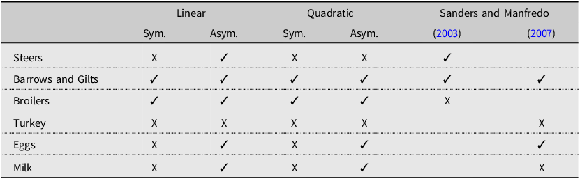
Table 3 reports our findings in relation to the previous work by Sanders and Manfredo (Reference Sanders and Manfredo2003) and Sanders and Manfredo (Reference Sanders and Manfredo2007). Examining the same price series from the third quarter of 1982 through the third quarter of 2002 (Sanders and Manfredo, Reference Sanders and Manfredo2003) or the third quarter of 2004 (Sanders and Manfredo, Reference Sanders and Manfredo2007), the previous studies found that the forecasts for steers, barrows and gilts, and eggs were optimal under a mean-zero quadratic loss function but reject the optimality of the forecasts for broilers, turkey, and milk. Using more recent data, from 1995 through 2024, we also find evidence in support of optimality under a mean-zero quadratic loss function for barrows and gilts, as well as broilers, which were previously rejected by Sanders and Manfredo (Reference Sanders and Manfredo2003). When evaluating optimality under the range of quadratic and linear loss functions, we also find evidence of optimality for USDA forecasts of eggs, which was optimal in Sanders and Manfredo (Reference Sanders and Manfredo2007), and milk, which was not optimal in Sanders and Manfredo (Reference Sanders and Manfredo2007). The forecast with the fewest cases of optimality was that of steer prices, which was optimal only under a set of asymmetric linear loss functions. Finally, we were unable to detect a range of optimality for USDA’s turkey price forecast, consistent with prior findings of Sanders and Manfredo (Reference Sanders and Manfredo2007).
Candidate loss functions for USDA forecasters of WASDE animal product price forecasts

Table 3 Long description
The table compares candidate loss functions for USDA forecasters of WASDE animal product price forecasts. It has six rows and five columns. The columns are labeled Linear Sym, Linear Asym, Quadratic Sym, Quadratic Asym, and Sanders and Manfredo. The rows are labeled Steers, Barrows and Gilts, Broilers, Turkey, Eggs, and Milk. The table shows whether each loss function is optimal for each animal product. For example, the forecast for steers is optimal under asymmetric linear loss functions, while the forecast for barrows and gilts is optimal under both symmetric and asymmetric quadratic loss functions. The table also includes findings from previous studies by Sanders and Manfredo in 2003 and 2007.
All results are reported at p < 0.05 significance value.
Source: Authors’ calculations are based on USDA WASDE 1995 to 2024 and Sanders and Manfredo (Reference Sanders and Manfredo2003) and Sanders and Manfredo (Reference Sanders and Manfredo2007).
Finally, it is important to note that, in addition to our primary analysis, we examine the optimality of the USDA animal product price forecasts using two-quarter and three-quarter-ahead rolling forecasts, and find similar results, which can be found in the Appendix.
4. Discussion
A number of prior studies suggest that USDA forecasts are not optimal. These studies employ a series of regression-based tests of the necessary conditions of forecast optimality, which implicitly assume a mean-zero quadratic loss function. While researchers typically conclude that a rejection of these necessary conditions stems from nonoptimality, others argue that failure may be the result of a misspecified test. More specifically, optimality is rejected because the forecasters are not minimizing a mean-zero quadratic loss function. This study proposes a alternative approach in how USDA forecasts may be evaluated by developing a method of identifying candidate loss functions for which the necessary conditions of optimality are satisfied. Our approach builds on the foundational forecast optimality test of Mincer and Zarnowitz (Reference Mincer, Zarnowitz, Mincer and Zarnowitz1969). Traditionally, the necessary conditions are tested using OLS, which implicitly assumes that the forecasters minimize a mean-zero quadratic loss function. Alternatively, our approach which builds on Guler et al. (Reference Guler, Ng and Xiao2017) uses quantile and expectile regression to identify the dimensions under which the necessary conditions of optimality hold across the conditional relationship between observed and forecasted values. This approach does not make strict assumptions about whether the loss function is quadratic or centered at zero.
We provide an illustration of how the loss functions under which the forecasts can be considered optimal vary across USDA animal product price forecasts. We apply our method to quarterly WASDE forecasts of animal product prices from quarter one 1995 to quarter two 2024. We find that optimality can not be rejected under the conventional mean-zero quadratic loss for the just two price series: (i) barrows and gilts and (ii) broilers. Alternatively, for eggs and milk, optimality holds for either linear or quadratic loss in a manner that places a greater weight on over-prediction errors relative to under-prediction. Steers are only optimal under a smaller set of candidate loss functions, those with linear loss that place a greater weight on over-prediction errors relative to under-prediction. Finally, we fail to identify a class of loss functions under which turkey price forecasts can be considered optimal. Thus, we argue that the USDA forecasters’ cost of forecast errors likely differs across these series.
Economic theory suggest that the loss functions may reflect a wide variety of costs or influences that are both internal or external to the forecaster. It is possible that various market forces or sources of information differ across these animal product forecasts, which may influence the properties of the forecasters’ loss function. For example, poultry markets are generally characterized by a large degree of vertical integration (O’Brien, Reference O’Brien2005). Vertical integration may, in turn, influence the information available to USDA forecasters or the use of the forecast by industry participants. Our illustration suggests future research could examine the characteristics of animal product markets and their influence on USDA forecasters’ loss function.
As previously noted, a forecast is only optimal for a specific forecast user if their loss function matches that of the forecaster (Auffhammer, Reference Auffhammer2007). Armed with a better understanding of the forecasters’ costs and how they guide the forecasting procedure, forecast users can better interpret the information provided by the forecast. For example, extension agents preparing their own forecasts or comparing their forecasts to the USDA will benefit from a better understanding of the costs experienced by USDA forecasters and how these costs may guide forecasting decisions. For example, our illustration suggests a number of forecasts may be considered optimal under loss functions that place a greater weight on over-prediction errors relative to under-prediction. Thus, USDA forecasters would prefer a forecast that under-predicts outcomes to one that over-predicts outcomes. As a result, the forecasts may be what Granger (Reference Granger1969) calls an optimally (downward) bias forecast. The extension forecaster without the same loss function may exhibit less bias compared to USDA forecasters.
Further, this alternative framework encourages USDA forecasters to think about their costs and how they guide their forecasting procedures. The status quo forecast evaluation approach assumes that these costs take a particular form, which may not represent those experienced by USDA forecasters. Thus, a more explicit documentation of these costs may be of value to forecast users and forecast evaluators.
Our illustration demonstrates that how USDA forecasters experience costs of forecast errors may vary across animal product price forecasts. Future research may similarly examine the degree to which these costs vary across other forecasts, such as crop price and production forecasts. The overlapping, fixed-event nature of crop forecasts may require adjustments to our empirical approach, however, which is left for future research.
Supplementary material
The supplementary material for this article can be found at https://doi.org/10.1017/aae.2025.10031.
Data availability statement
The data used in this study is available.
Author contributions
Conceptualization: C.F. and T.K.; Methodology: C.F., T.K., and S.B.; Formal Analysis: C.F., T.K., and S.B.; Data Curation: S.B.; Writing – Original Draft: C.F., T.K., and S.B.; Writing – Review and Editing: C.F., T.K., and S.B.; Supervision: C.F., T.K., and S.B.; Funding Acquisition: NA.
Financial support
Dr Siddhartha Bora’s work was supported in part by USDA-NIFA Hatch Project #WVA00779. Drs. Fiechter and Kuethe research received no specific grant from any funding agency, commercial or not-for-profit sectors.
AI statement
AI editing assistant Writefull was used in generating the manuscript.
Chad Fiechter is an Assistant Professor of Agricultural Finance at Purdue University. His primary research areas include agricultural finance, farm management, and production economics.
Siddhartha S. Bora is an Assistant Professor of Agribusiness Management and Applied Economics at West Virginia University. His primary research areas include commodity markets, natural resources, time-series analysis, and big data analytics. He holds a Ph.D. in Agricultural Economics from The Ohio State University.
Todd H. Kuethe is a Professor and Schrader Chair in Farmland Economics at Purdue University. His primary research areas are agricultural finance and agricultural policy. He holds a PhD from Purdue University.


 Open access