

1. INTRODUCTION
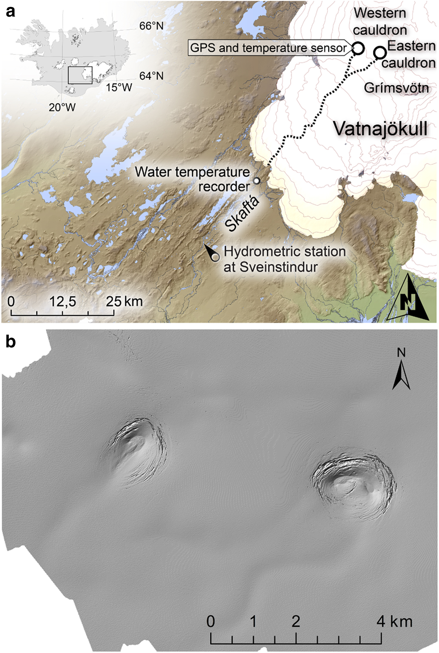
Jökulhlaups in the river Skaftá from western Vatnajökull occur at 1–2 year intervals with volumes of 0.05–0.4 km3 and maximum discharge of 50–3000 m3 s–1 (Björnsson, Reference Björnsson1977; Zóphóníasson, Reference Zóphóníasson2002; unpublished data from the Icelandic Meteorological Office). The floods originate from two subglacial lakes below 50–150 m deep and 1–3 km wide depressions (cauldrons) in the ~450 m thick surrounding ice cap. Together, the depressions drain ~50 km2 of the ice cap (Pálsson and others, Reference Pálsson, Björnsson, Haraldsson and Magnússon2006) (Fig. 1). The jökulhlaups travel ~40 km subglacially before they emerge at the terminus of the outlet glacier Skaftárjökull.
(a) The Skaftá cauldrons and subglacial lakes in the western Vatnajökull ice cap and the upper part of the watershed of the Skaftá river. The inferred subglacial paths of jökulhlaups (dotted lines) and locations of instruments described in the text are shown. (b) A hillshade of a DEM of the cauldron area measured by lidar (acronym for ‘light detection and ranging’) in 2010.
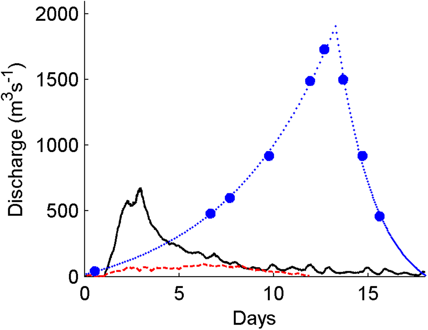
Jökulhlaups in Skaftá reach maximum discharge in 1–3 days and typically recede in 1–2 weeks (Björnsson, Reference Björnsson2002) (Fig. 2). They are on the ‘rapidly rising’ side of the spectrum of ‘rapidly rising’ to ‘slowly rising’ jökulhlaups (Einarsson and others, Reference Einarsson2016). The hydrograph of slowly rising jökulhlaups, such as most floods from Grímsvötn subglacial lake in Vatnajökull, gradually rises to maximum discharge in 1–3 weeks and recedes in <1 week, often in only 1–3 days (Björnsson, Reference Björnsson2002) (Fig. 2). Jökulhlaups from subglacial and marginal lakes at other locations in Iceland may rise even more rapidly than jökulhlaups in Skaftá and can reach maximum discharge in less than half a day (Thórarinsson, Reference Thórarinsson1974; Sigurðsson and Einarsson, Reference Sigurðsson and Einarsson2005; Jónsson and Þórarinsdóttir, Reference Jónsson and Þórarinsdóttir2011). The hydrographs of slowly rising jökulhlaups are reasonably well explained by the theory of conduit-melt–discharge feedback, developed by Nye (Reference Nye1976). The rapid initial increase of the hydrograph during jökulhlaups in Skaftá is difficult to explain with Nye's theory without invoking implausibly high temperature for the lake water (Björnsson, Reference Björnsson1992), and many aspects of the dynamics of rapidly rising jökulhlaups are still unresolved. As rapidly rising jökulhlaups have a fast discharge increase, they may be extremely dangerous since warning times for response are short.
Comparison of the hydrographs of a large rapidly rising jökulhlaup in 2002 (solid curve) and the small jökulhlaup in 2006 with a rapid initial rise, which is the subject of this paper (dashed curve), both from the western Skaftá cauldron. The hydrograph of a typical slowly rising jökulhlaup from Grímsvötn in 1986 (dotted curve) is also shown. The hydrograph of the Grímsvötn jökulhlaup is based on discrete discharge measurements which are shown as dots. The rapid rise of the hydrograph of the 2006 jökulhlaup is more clearly visible in Figure 6 which shows the same discharge curve with the vertical scale expanded.
The fundamental reasons that govern whether a jökulhlaup develops as a rapidly rising or slowly rising flood are not fully understood. The predominant discharge development mechanism appears to be different for these two types of floods. Hydraulic uplift of the glacier, caused by water pressure exceeding glacier overburden pressure in a propagating subglacial pressure wave, is likely to be an important component in the flood path formation for rapidly rising jökulhlaups (Björnsson, Reference Björnsson2002; Jóhannesson, Reference Jóhannesson2002; Flowers and others, Reference Flowers, Björnsson, Pálsson and Clarke2004; Roberts, Reference Roberts2005; Einarsson and others, Reference Einarsson2016). Flood path formation by coupled subglacial sheet of water and conduit flow has been used for modelling of rapidly rising jökulhlaups (Flowers and others, Reference Flowers, Björnsson, Pálsson and Clarke2004). The formation of the initial sheet has been proposed to be caused by ice dam flotation near the subglacial lake (Björnsson, Reference Björnsson2002, Reference Björnsson2010; Flowers and others, Reference Flowers, Björnsson, Pálsson and Clarke2004; Sugiyama and others, Reference Sugiyama, Bauder, Huss, Riesen and Funk2008) and hydraulic jacking along the flood path (Flowers and others, Reference Flowers, Björnsson, Pálsson and Clarke2004). Positive feedback between discharge and melting in the sheet leads to the creation of conduits that carry an increasing proportion of the water as the flood develops. The subglacial flood path of slowly rising jökulhlaups is, on the other hand, thought to be mainly formed by melting by frictional heat released in the flow by dissipation of potential energy and the initial heat of the source water (Nye, Reference Nye1976; Spring and Hutter, Reference Spring and Hutter1981, Reference Spring and Hutter1982). Recent research on jökulhlaups from Grímsvötn indicates that lifting of the glacier may also play a role in flood path formation of some slowly rising jökulhlaups (Björnsson, Reference Björnsson2010; Magnússon and others, Reference Magnússon2011; Einarsson and others, Reference Einarsson2016).
The discharge development of a jökulhlaup seems to depend on both local conditions at each site and the initial conditions for each particular flood. Both rapidly rising and slowly rising jökulhlaups can originate from the same source location. As an example, the 1861, 1892, 1938 and the November 1996 jökulhlaups from Grímsvötn in Vatnajökull were all of the rapidly rising type (Thórarinsson, Reference Thórarinsson1974; Björnsson, Reference Björnsson2002), whereas over 20 jökulhlaups from Grímsvötn in the decades from 1940 to 2010 were slowly rising (Thórarinsson, Reference Thórarinsson1974; Björnsson, Reference Björnsson2002; Sigurðsson and Einarsson, Reference Sigurðsson and Einarsson2005; unpublished data from the Icelandic Meteorological Office). Different drainage mechanisms for different outbursts from the same source location have likewise been identified for Gornersee in Switzerland (Huss and others, Reference Huss, Bauder, Werder, Funk and Hock2007).
Subglacial water flow and variations in subglacial water pressure have attracted increasing attention in recent years as a likely cause of the large variations in ice flow velocities that have been observed on the main outlets of the Greenland ice sheet and some of the ice streams of Antarctica (e.g. Rignot and Kanagaratnam, Reference Rignot and Kanagaratnam2006; Fricker and others, Reference Fricker, Scambos, Bindschadler and Padman2007; Stearns and others, Reference Stearns, Smith and Hamilton2008; Doyle and others, Reference Doyle2015). Subglacial accumulation of water has been observed or inferred at many locations on large and small glaciers and found to be associated with substantial increases in ice flow velocities (e.g. Iken and Bindschadler, Reference Iken and Bindschadler1986; Fudge and others, Reference Fudge, Harper, Humphrey and Pfeffer2009; Magnússon and others, Reference Magnússon2011). Jökulhlaups provide one of the best opportunities to study the response of the subglacial hydraulic system to large and sudden variations in water flow, and lessons learned from studies of jökulhlaups may be useful for understanding variations in basal sliding and ice flow in glaciers and ice sheets in general (Bell, Reference Bell2008).
To gain understanding of the energy balance, heat dissipation and flood path formation and development in rapidly rising jökulhlaups, a campaign to monitor the Skaftá cauldrons and the Skaftá river was initiated in 2006. This paper reports our results on the subglacial hydrology of the September 2006 jökulhlaup from the western Skaftá cauldron. Outflow from the subglacial lake and transient storage of water in the subglacial flood path are derived and used, together with water temperature measurements in the subglacial lake and near the terminus, to shed light on the dynamics of the flood path development for this type of flood. The emptying of a cylindrically symmetric subglacial lake is simulated with the full-Stokes ice-dynamic model Elmer/Ice (Gagliardini and others, Reference Gagliardini2013) to deduce a relationship between water volume in the lake and ice-shelf elevation for calculations of outflow from the lake and for analysing the size of the subglacial lake in relation to the observed dimensions of the ice-surface depression.
2. DATA AND METHODS
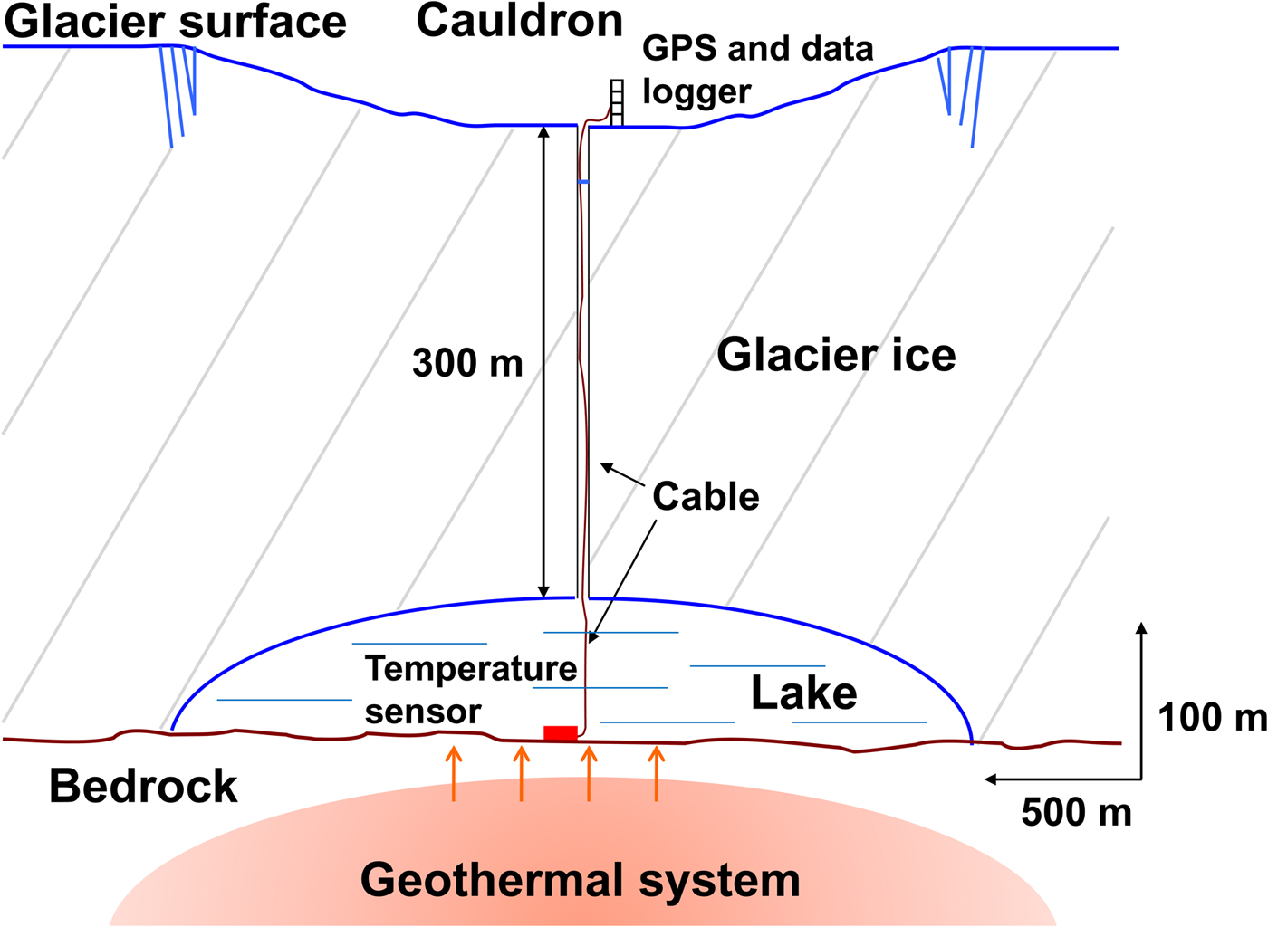
The ice shelf covering the western Skaftá cauldron was penetrated by a hot water drill in June 2006 (Thorsteinsson and others, Reference Thorsteinsson2007). (The term ‘ice shelf’ is used in this paper to describe the ice cover overlying the subglacial lakes as the weight of the ice is to a large extent supported by flotation. The ice shelves are, however, fundamentally different from the large ice shelves at the margins of ice sheets and glaciers in, for example, Antarctica, Greenland and Canada.) A temperature sensor was deployed at the bottom of the lake and connected with a cable to a data logger on the surface (Fig. 3). A differential GPS instrument was placed at the centre of the cauldron, and a water temperature logger was placed in the Skaftá river, 3 km downstream of the port where the river emerges from beneath the ice (Fig. 1).
Schematic drawing of the western Skaftá cauldron showing the ~300 m thick floating ice shelf penetrated by a drillhole into the ~100 m deep subglacial lake and the scientific instruments deployed in the lake and on the glacier surface in the campaign in 2006. Note that the vertical scale is exaggerated five-fold.
2.1. Proglacial discharge
The proglacial discharge in Skaftá was measured at the hydrometric station at Sveinstindur, 25 km downstream of the glacier margin. The discharge at the river outlet at the glacier terminus was back-calculated with flood routing using the 1-D HEC-RAS hydraulic model for unsteady flow in open channels (Jónsson, Reference Jónsson2007). In addition to the jökulhlaup component, the discharge measured at Sveinstindur includes the normal discharge from the glacier and from several relatively small tributaries. These additional discharge components were estimated, based on a comparison with river discharge records for similar weather conditions, and subtracted from the measured discharge to yield a discharge estimate for the flood originating from the cauldron (Einarsson, Reference Einarsson2009). The uncertainty in this discharge estimate arises from the uncertainty of the discharge measurement at Sveinstindur and the uncertainties of the estimates for base flow and for rain and melt-induced runoff from the watershed during the period 26 September to 2 October. The uncertainties of the base flow (±5 m3 s–1) and rain and melt runoff (±10 m3 s–1) are relatively large for this small jökulhlaup in 2006, compared with the uncertainty of discharge measurement at Sveinstindur (±2%; see Jónsdóttir and others, Reference Jónsdóttir, Kristjánsdóttir and Zóphóníasson2001). This leads to ±12 m3 s–1 uncertainty in the jökulhlaup discharge and ±20% uncertainty in the estimated flood volume and rate of outflow from the subglacial lake because subtraction of base flow and melt-induced runoff increases the relative uncertainty in the final results.
2.2. Glacier surface elevation over the subglacial lake
The elevation of the ice shelf varies in response to changes in the volume of water in the subglacial lake. The elevation of the surface of the ice shelf was measured near the centre of the cauldron with a Trimble 4000SE GPS receiver equipped with a Trimble 4000ST L1 Geodetic antenna. The receiver logged data at 15 seconds intervals for 5 minutes at 08:00 every morning. The average of the measurements from each 5 minutes logging interval provided one GPS location per day during the period 14 September to 25 October. The data were processed with the Trimble Geomatics Office software using base station data from the stations GFUM (Grímsfjall, length of baseline ~20 km) and SKRO (Skrokkalda, length of baseline ~37 km). Based on fluctuations in the measurements between adjacent days during time periods of slow vertical movements before and after the jökulhlaup, the relative accuracy of the measured surface elevation is estimated to be <1 m.
2.3. The geometry of the cauldron and the subglacial lake
The difference of two 5 m × 5 m DEMs of the cauldron between filled and empty stages was used to deduce the geometry of the part of the subglacial volume that is emptied out in jökulhlaups. A DEM based on aerial synthetic aperture radar (SAR) measurements from August 1998 was made of western Vatnajökull by Magnússon (Reference Magnússon2003). A jökulhlaup with a peak discharge of 149 m3 s–1 and total volume of 0.116 km3 drained from the western cauldron in September 1998, <1 month after the aerial survey, so the western cauldron was nearly filled at the time of the survey. A second DEM of the Skaftá cauldron area was made with airborne lidar in July 2010 (Jóhannesson and others, Reference Jóhannesson2013). The western cauldron was at a low water level at the time of the lidar survey, as a jökulhlaup with a peak discharge of ~410 m3 s–1 and total volume of 0.190 km3 drained the western cauldron in June 2010, ~1 month before the survey.
Our inferred geometry of the subglacial volume is not based on direct measurements immediately before and after the 2006 flood and may be affected by changes in ice thickness in the 12 years between the SAR and lidar ice-surface measurements in 1998 and 2010 when seven other jökulhlaups are recorded (Zóphóníasson, Reference Zóphóníasson2002; unpublished data from the Icelandic Meteorological Office). The shape of the ice surface of the western cauldron shortly before a jökulhlaup is flat and smooth and is expected to be very similar for different floods. The general size and shape of the cauldron at the end of a jökulhlaup has been monitored from many reconnaissance flights during and after the floods and is also found to be rather similar for the events that have been observed (O. Sigurðsson, personal communication, 2016). The geometry of ice thickness changes over the subglacial lake in a jökulhlaup cycle are therefore expected to be rather similar between cycles. The general lowering of the glacier surface due to a negative mass balance since 1998 is accounted for by subtracting the elevation difference in the adjacent area unaffected by the cauldron subsidence. The subglacial lake is not fully emptied out in jökulhlaups so that large parts of the ice shelf do not touch the underlying bedrock at the end of the floods. Small-scale transient changes due to melting at the underside of the ice shelf, caused by possible spatial variations in the subglacial geothermal activity, are, therefore, not expected to affect the inferred geometry of the volume that is emptied out in jökulhlaups. The inferred geometry of the subglacial volume is affected by a hump near the centre of the cauldron. The hump is most likely an ice-dynamic thrust phenomenon connected to ice flow into the cauldron and therefore does not represent the shape of the subglacial lake. This effect is small compared with other uncertainties in the estimation of the geometry of the lake.
2.4. The hypsometry of the subglacial lake
The water volume in the subglacial lake is not a simple function of the lake geometry and water level as for lakes in bedrock basins because the geometry of the lake may change with the ice-shelf elevation. A hypsometric curve, i.e. lake water volume as a function of ice-shelf elevation, for the lowering of the ice shelf was calculated with the full-Stokes ice-dynamic model Elmer/Ice (Gagliardini and others, Reference Gagliardini2013) by simulating the emptying of a cylindrically symmetric subglacial lake below an ice cover with the approximate dimensions of the western Skaftá cauldron. The question to be addressed by the simulation is whether the subglacial water body maintains a similar shape as the ice shelf is lowered and the lake is emptied or whether the lake geometry changes substantially due to internal shear within the ice shelf near the lake edge such that the grounding line at the lateral boundary moves inward as the shelf lowers. These two possibilities correspond to different relationships between the rate of lowering of the ice shelf and the rate of outflow from the subglacial lake, leading to different trajectories between the two known points on the volume–ice-shelf-elevation curve that are determined by the observed total outflow and surface lowering. Our modelling is simplistic and meant to capture the main physical processes that determine the shape of the hypsometric curve but not the 2006 event in detail. The model setup is, thus, based on a simplified geometry of the western cauldron and general characteristics of jökulhlaups released from there and the final results are scaled to the observed volume and ice shelf lowering in the 2006 event. The physical basis of our model formulation is in principle similar to the analytical model of cauldron subsidence during jökulhlaups developed by Evatt and Fowler (Reference Evatt and Fowler2007) but there are differences in the geometrical and physical assumptions as will be further described in Section 4.
The Skaftá cauldrons and ice flow in their vicinity are close to being cylindrically symmetric in geometry (Figs 1 and 3). A cylindrically symmetric model configuration was chosen because the detailed geometry of the ice-flow basin away from the subglacial lake, which deviates from cylindrical symmetry, is not expected to influence the form of the calculated hypsometric curve to a significant degree.
We take the overall shape and size of the subglacial lake as given, based on the inferred geometry of the volume emptied out in the 2010 jökulhlaup. This shape is dynamically determined over many jökulhlaup cycles and it is outside the scope of this paper to derive and analyse this time-dependent geometry by modelling. The modelled lake is assumed to have a convex shape and maximum depth of ~100 m at the centre at the start of a jökulhlaup and to be covered with an ice shelf with surface geometry based on the 1998 SAR DEM (see Fig. 4, which explains the notation used to describe the model geometry). The glacier and the lake are underlain by flat bedrock in the model set-up.
The Elmer/Ice computational finite-element mesh for the cylindrically symmetric model of a glacier on a flat bed overlying a subglacial lake with dimensions corresponding to the western Skaftá cauldron. The figure explains the notation used to define the geometry of the model: the elevation of the ice surface, z s, and the bottom of the ice, z b, the time-dependent piezometric water level of the subglacial water lake, z w, the radial distance to the grounding line, r l, the radius of the geothermal area, r g, the radius to the ice divide at the boundary of the cauldron ice flow basin with the surrounding ice cap, r d and the ice-surface elevation at the ice divide, z d. A jökulhlaup is released when z w reaches a critical level z 1 and terminated when z w reaches z 2.
The dynamic and kinematic boundary conditions at the ice surface and the ice/bed interface are formulated with a stress-free upper surface, as is customary in ice flow models of this kind (e.g. Gagliardini and others, Reference Gagliardini2013), and a constant uniform positive surface mass balance b s. The stress-free upper surface is assumed to have a smooth geometry, ignoring the dynamic effect of surface crevasses that are observed to be formed in a concentric pattern during the subsidence of the ice shelf. The lidar measurements in 2010, shortly after a jökulhlaup, showed crevasse depths up to 40 m, which should be considered a minimum as the lidar is not likely to have reached to the bottom of the deepest crevasses. Crevasses formed over a timescale of several days during a jökulhlaup may be estimated to be on the order of 100 m deep (Cuffey and Paterson, Reference Cuffey and Paterson2010, Eqn (10.6), p. 449). As the surrounding glacier is ~450 m thick, the crevasses may have some effect on the ice dynamics but neglecting them is not likely to have a dominating effect on our results considering other simplifications in our modelling specification.
The kinematic boundary condition at the bottom of the ice takes geothermal melting of ice, m g, into account within the radius of the geothermal area r g. The dynamic boundary condition at the ice/bed interface assumes Weertman sliding,  $u_{\rm b} = C{\kern 1pt} \tau _{\rm b}^{m - 1} {\kern 1pt} \tau _{\rm b}$, where u b is the bed-parallel velocity component, τ b is the basal shear stress and C and m are parameters.
Water pressure in the lake, p w, is assumed to be hydrostatic:
 $$p_{\rm w} = \rho _{\rm w}{\kern 1pt} g{\kern 1pt} (z_{\rm w} - z), $$
where z w is the piezometric height of the lake, and the dynamic boundary condition at the ice/water interface is formulated in terms of the water pressure that is set equal to the (negative of the) surface normal stress in the ice at the shear-stress-free bottom of the ice shelf. The position of the grounding line, where the ice/water interface meets the ice/bed interface, is part of the solution and evolves with time. Its position at each time step is determined by solving a contact problem. At each node, the normal force exerted by the ice on the bedrock is compared with the water pressure at that location and the ice allowed to separate from the bed in case the water pressure is higher (see Gagliardini and others, Reference Gagliardini2013).
The lake is assumed to be hydraulically connected to the atmosphere through water passageways such as crevasses or moulins. The volume of water in the lake and surrounding waterways, V w, is the sum of (i) the lake volume, taken to be the integral of the elevation of the bottom of the ice shelf, z b, over the area of the lake, and (ii) the water volume in the passageways between the lake and the atmosphere, which we assume can be expressed as water level in the passageways, z w, multiplied with their effective area, S, by analogy with the traditional way to express ground water storage in terms of a storage coefficient (Fetter, Reference Fetter2001). Therefore, variations in V w, may be expressed as
 $$\displaystyle{{{\rm d}V_{\rm w}} \over {{\rm d}t}} = \int_0^{r_{\rm l}} {\kern 1pt} \displaystyle{{{\rm d}z_{\rm b}} \over {{\rm d}t}}{\kern 1pt} 2{\kern 1pt} \pi {\kern 1pt} r{\kern 1pt} {\rm d}r + S\displaystyle{{{\rm d}z_{\rm w}} \over {{\rm d}t}} = q_{\rm s} + q_{\rm f} + q_{\rm g} - q_{\rm j}, $$
where the flux components q s, q f, q g and q j on the right-hand side are inflow into the lake due to surface melting and rainfall on the surface, inflow of geothermal fluid, basal geothermal melting and rate of outflow from the lake during jökulhlaups, respectively. This equation is solved for z w with explicit forward time stepping in such a way that the flux components, as well as simulated changes in the ice-shelf geometry, force changes in water pressure through adjustment of the piezometric height of the lake that induce further changes in the ice-shelf geometry through the dynamic boundary condition at the ice/water interface in a feedback loop. Each time step of the modelling involves an update of the mesh, calculation of the area where the glacier is grounded and an update of the piezometric height of the lake based on the previous geometry and the flux components. Changes in normal pressure at the ice/water interface due to variations in the piezometric height lead to stresses and strains in the ice, and the resulting ice motion drives changes in the volume of the subglacial water body that subsequently lead to changes in the piezometric height and grounding line position in the next time step. Because of the very different timescales for filling and emptying of the lake between and during jökulhlaups, variable-length time stepping was implemented with time steps switching between the order of hours between jökulhlaups and the order of minutes during jökulhlaups.
Surface mass balance over the ice flow basin, b s, the rate of geothermal melting of ice, m g and the rate of inflow of geothermal fluid from the geothermal system, q f, are estimated from mass and energy conservation assuming long-term balance of total precipitation over the ice flow basin with area  $A_{\rm i} = \pi {\kern 1pt} r_{\rm d}^2 $, bottom geothermal melting over an area $A_{\rm g} = \pi {\kern 1pt} r_{\rm g}^2 $ and outflow in jökulhlaups when averaged over many jökulhlaup cycles as in Jóhannesson and others (Reference Jóhannesson, Thorsteinsson, Stefánsson, Gaidos and Einarsson2007). The flux components q s and q g in Eqn (2) are assumed to be constant in time, ignoring the seasonal mass-balance cycle, which is not expected to be important for the emptying of the lake. The rate of jökulhlaup outflow, q j, is assumed to rise linearly with time from zero to a constant discharge q k over a time period t r and fall linearly to zero over a time period t f when the piezometric water level in the subglacial lake rises or falls to the thresholds z 1 and z 2, respectively (see Fig. 4). Table 1 gives the values used for model geometry and physical constants in the simulations.
Parameters defining an idealized, cylindrically symmetric model for the western Skaftá cauldron
Several model parameters are not well constrained by available observations or theory, in particular the parameters describing the geothermal melting, A g (and consequently m g), the timescales for the rise and fall of the jökulhlaup discharge, t r and t f, the effective area of the assumed hydraulic connection with the atmosphere, S, as well as the sliding parameters C and m. The numerical values of the parameters A g, t r, t f and S as well as the grid resolution were varied by a factor of 2–100 to test the sensitivity of the model, and no significant changes in simulation results occurred. For computational reasons, the adopted values of S are large compared with the expected magnitude of water passageways through bottom channels, englacial cavities and crevasses. Varying S by two orders of magnitude made little difference to model results, indicating that this parameter only affects the resulting hypsometric curve to a small degree.
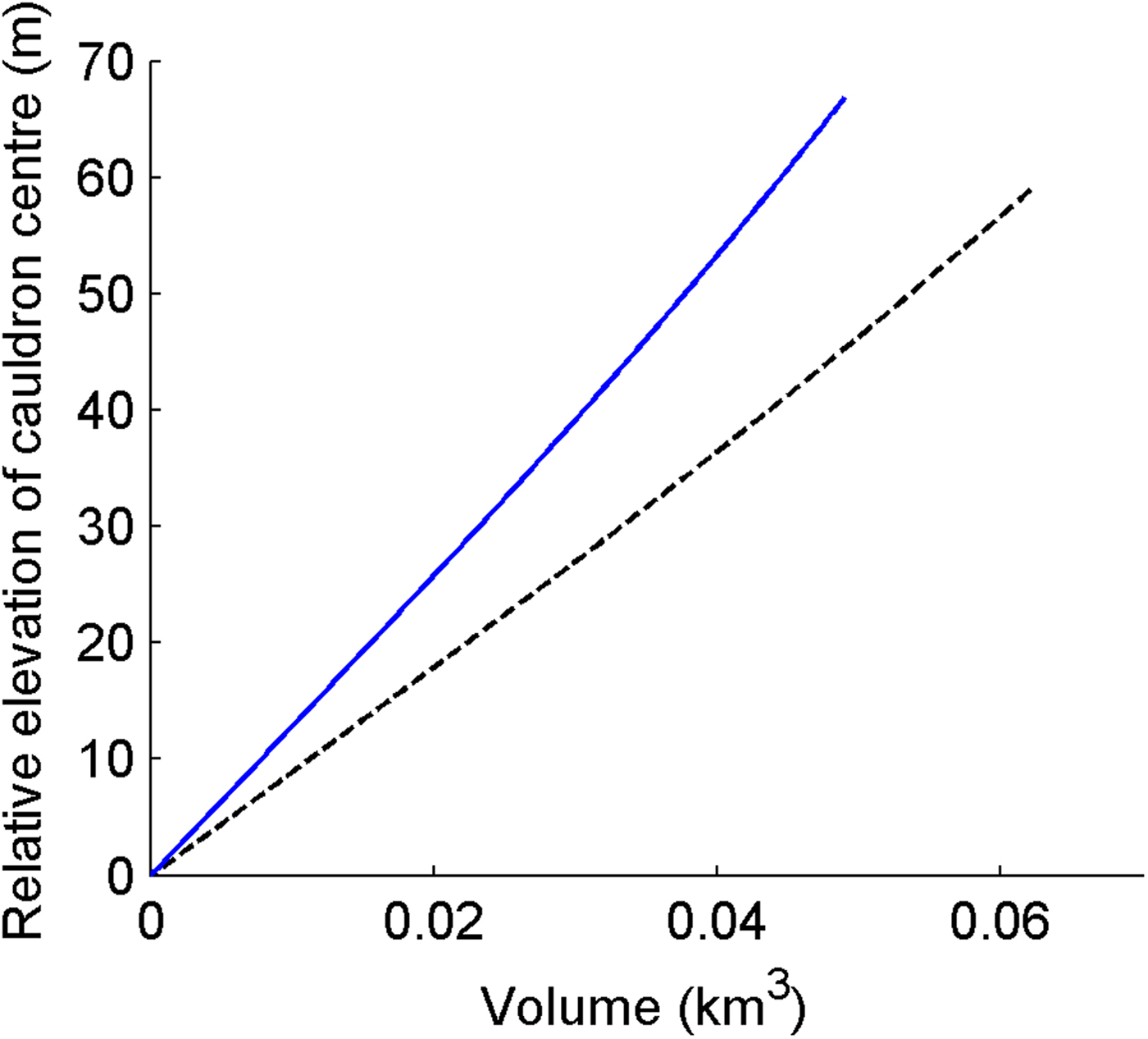
The resulting hypsometric curve shows an approximately linear relation between ice-shelf elevation and lake water volume (Fig. 5, dashed curve), indicating that the subglacial water body maintains a similar shape as the ice shelf is lowered. The simulated hypsometric curve was scaled to fit the observed values for total outflow volume and surface lowering during the 2006 jökulhlaup, allowing the calculation of outflow discharge as a function of time based on the measured lowering of the ice shelf during the flood.
Hypsometric curves for the subglacial lake below the western Skaftá cauldron showing lake volume as a function of the elevation of the cauldron centre. The result of the Elmer/Ice modelling (dashed curve) and a scaled curve that fits the observed flood volume vs. ice-shelf lowering in the September/October 2006 jökulhlaup (solid curve) are shown.
2.5. Floodwater temperature and energy available for subglacial melting
Continuous measurements of water temperature in Skaftá river were made at Fagrihvammur, 3 km downstream of the glacier margin (Fig. 1), during the September/October 2006 jökulhlaup, using a Starmon mini temperature recorder with an accuracy of ± 0.1°C. The measurements, as well as an evaluation of potential warming over the 3 km distance from the glacier margin to the measurement site, are described by Einarsson (Reference Einarsson2009). Discrete measurements of floodwater temperature at the glacier margin in jökulhlaups in Skaftá in August and October 2008 and October 2015 were made with a high-precision RBR thermometer, with an accuracy of ± 0.005°C. Measurements of water temperature in the subglacial lake of the western cauldron in June 2006 are described by Jóhannesson and others (Reference Jóhannesson, Thorsteinsson, Stefánsson, Gaidos and Einarsson2007).
The energy available for melting of ice along the subglacial flood path until a particular point in time after the floods starts may be used to calculate an upper bound on the volume of the flood path that can have been created by melting at that time
 $$V_{{\rm melt}} = \displaystyle{{c_{\rm w}\rho _{\rm w}V_{\rm l}T_{\rm l} + g\rho _{\rm w}V_{\rm l}\Delta H - c_{\rm w}\rho _{\rm w}V_{\rm s}T_{\rm s}} \over {L\rho _{\rm i}}},$$
where g is the acceleration of gravity and ρ w, c w, ρ i and L are the density and the heat capacity of water, and the density and latent heat of fusion of ice, respectively (Table 2). T l and T s are the temperature of the floodwater in the lake and at the glacier snout. ΔH is the elevation difference between the water level in the subglacial lake and the glacier snout (815 m for the flood path from the western Skaftá cauldron, Einarsson, Reference Einarsson2009). Finally V l and V s are the volumes of water released from the subglacial lake and at the glacier snout up to the time in question. The first term in the numerator on the right-hand side of the equation is the available thermal energy due to the initial heat of the water in the lake, the second term is the available potential energy and the third term is the thermal energy left in the water at the glacier snout. The kinetic energy in the water flow at the glacier snout is neglected as it is small compared with the other terms. This volume estimate is an upper bound as the potential energy component corresponds to flow all the way from the lake to the outlet and the thermal energy corresponding to the deviation of the subglacial floodwater temperature from the freezing point upstream from the snout is included in the estimate of the available energy.
Physical parameters used in melt volume calculations
3. RESULTS
3.1. Proglacial discharge
A rapidly rising jökulhlaup from the western Skaftá cauldron emerged at the glacier margin on 27 September 2006, reaching a maximum discharge close to 100 m3 s–1 in ~2 days. It had the typical form of small jökulhlaups from the western cauldron, with a relatively flat discharge maximum for ~6 days, and receded in ~4 days. The back-calculated flood discharge at the glacier terminus (Fig. 6, solid curve), after subtraction of the base flow, reached its maximum of ≈97 m3 s–1 in the afternoon of 2 October. As the estimation of the time-varying base flow is uncertain, the true discharge maximum might have occurred in the interval 29 September to 2 October, but the maximum value of ≈100 m3 s–1 is fairly accurate as the discharge peak was broad and flat.
Back-calculated discharge of jökulhlaup water (solid curve) at the glacier terminus during the jökulhlaup in September/October 2006 after subtracting base flow from the glacier and tributary rivers upstream of the Sveinstindur hydrometric station. The relative elevation of the cauldron centre, as measured with GPS, is also shown (dashed curve) as well as the calculated outflow from the subglacial lake (dash-dotted curve) derived from the lowering of the ice surface elevation using the hypsometric curve for the subglacial lake.
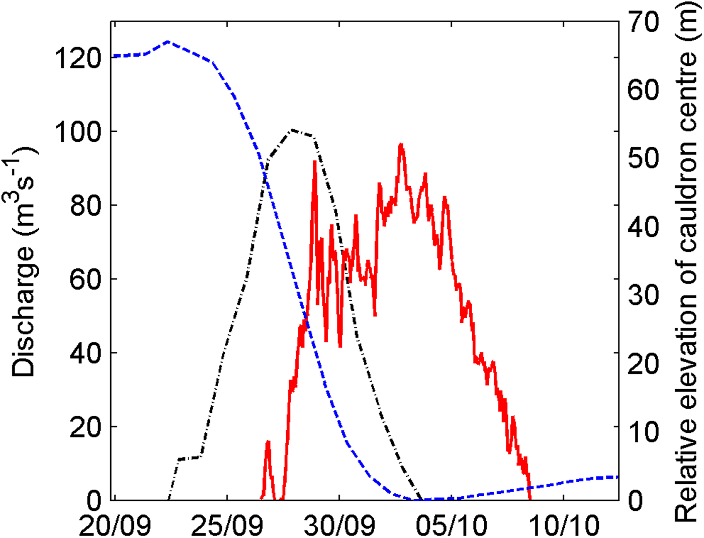
As for other jökulhlaups from the Skaftá cauldrons, the rapid rise in flood discharge during the first 2 days cannot be described by classic jökulhlaup theory (Björnsson, Reference Björnsson1977, Reference Björnsson1992; Sigurðsson and Einarsson, Reference Sigurðsson and Einarsson2005). Using model parameters based on the geometry of the flood path and channel roughness n m (Manning's roughness) in the range 0.01–0.1 s m–1/3, as reported for subglacial conditions by Cuffey and Paterson (Reference Cuffey and Paterson2010), the classic theory implies that the discharge should increase by a factor of 2 in the range of 1–7 days for discharge between 20 and 80 m3 s–1. The discharge, however, increased from ~20 to ~40 m3 s–1 in approximately half a day and from ~40 to ~80 m3 s–1 in less than a day. The form of the discharge variation is also far from the nearly exponential concave shape typical for slowly rising jökulhlaups (Fig. 6).
3.2. The geometry of the cauldron, the subglacial lake and the adjacent flood path
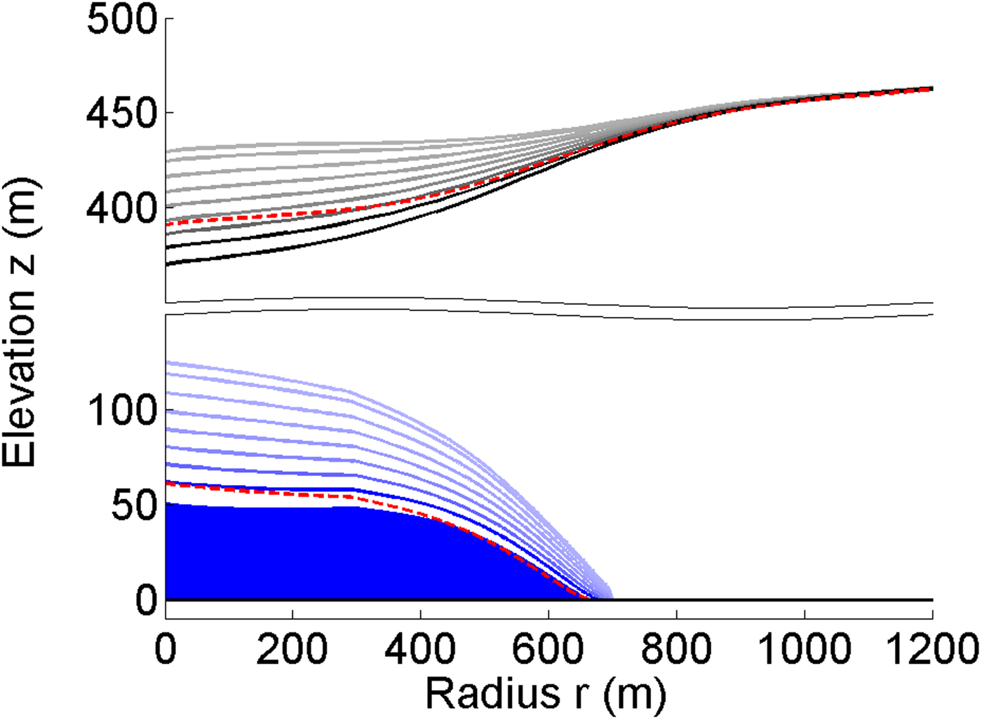
Inward movement of the grounding line in the modelled lowering of the ice shelf (Fig. 7) is minimal, ~40 m and the water depth is reduced in approximately the same proportion everywhere during outflow. The lake shape for different stages is therefore similar, leading to the approximately linear hypsometric curve shown in Figure 5. This indicates that the shelf has a substantial internal strength and shear stress support at the sides. We find that the water pressure at the bottom of the ice shelf in the centre of the cauldron falls below the ice overburden (positive effective pressure at the top of the subglacial cavity) by 0.2–0.4 MPa during the main outflow phase. This imbalance is compensated by a bridging shear stress of 0.15–0.3 MPa at the margins of the ice shelf. The modelling, furthermore, shows considerable thickening of the ice shelf during subsidence, which also affects the time-dependent shape of the lake (Fig. 7). This thickening from 305 to 320 m is caused by increased ice flow towards the centre during subsidence. The ice flow is increased both because of increased surface slope of the cauldron and shear softening of the glacier ice. The shear softening is caused by higher shear stresses in the ice shelf as support from the water pressure in the lake is reduced. The linear shape of the hypsometric curve is, thus, a net result of complex ice dynamics where both lateral support and vertical extension play a role. The reciprocal of the slope of a straight line, fitted to the hypsometry (Fig. 5), is the ‘effective’ area of the lake, if it were being emptied in a piston-like manner. This area, 1 km2, is smaller than the 1.5 km2 initial area of the modelled lake and relatively constant during lowering. The lowering of the surface of the cauldron affects an area substantially larger than the subglacial lake so that the surface lowering at the lake edge is ~20% of the maximum lowering at the centre. The modelled surface lowering is more than 1 m at a radius of 1050 m, 1.5 times the initial radius of the lake.
Lake and surface geometry during a jökulhlaup modelled with Elmer/Ice. The geometry is drawn at daily intervals with darker colour as time progresses. The lake and surface geometries 1 month after the end of the jökulhlaup are also drawn (dashed curves).
The subtraction of the SAR and lidar DEMs from 1998 and 2010 indicates a subglacial water body with a smooth, approximately cylindrically symmetrical shape (Fig. 8). The area that subsided is ~2.5 km in diameter, with maximum depth of ~90 m near the centre of the cauldron. The elongated shapes that appear on the flanks of the central water cupola are due to surface crevasses represented in the 2010 lidar DEM that were formed or enhanced during the July 2010 jökulhlaup. These shapes are thus not surface topography expressions of variations in subglacial lake depth. The modelled lowering of the ice shelf indicates that the margins of the ice surface depression with comparatively little difference in elevation between 2010 and 1998 (Fig. 8) are formed by ice dynamics during the lowering of the ice shelf and by ice flow into the cauldron over the month that elapsed from the jökulhlaup in June 2010 to the lidar survey in July (Fig. 7). The true width of the subglacial lake before a jökulhlaup may thus be expected to be smaller than shown in Figure 8.
(a) A hillshade of the difference between the adjusted 1998 SAR DEM and the 2010 lidar DEM. (b) A contour map of the inferred depth of the subglacial water body emptied in the 2010 flood, contour interval of 5 m. The data are smoothed with a 100 m × 100 m window.
Melting over the subglacial flood path has created an elongated depression in the outlet area of the cauldron, visible as the extension to the southwest from the area of the western cauldron in Figure 1b. The depression is deeper shortly after a jökulhlaup (as in 2010) than shortly before a jökulhlaup (as in 1998) and has been observed to be bounded by thin belts of narrow crevasses on each side after jökulhlaups (O. Sigurðsson, personal communication, 2008), indicating subsidence of the glacier surface along the depression. The ice surface elevation difference indicates that an ice volume ~10 m high, a few hundred metres wide and ~3 km long, which takes the shape of a ridge in Figure 8, is melted as the depression is formed during the initial stage of a jökulhlaup. Due to smoothing caused by ice dynamics the true geometry of the subglacial volume could be narrower and higher.
3.3. The water level and the depth of the subglacial lake
The water level in the borehole was at 1488 m a.s.l. at the time of the instrument set-up in June 2006, which is ~5 m higher than the level corresponding to flotation of the central part of the shelf. This deviation from floating balance means that an excess pressure of ~0.05 MPa was acting on the underside of the ice shelf near the centre (Einarsson, Reference Einarsson2009). The ice shelf rose slowly by 12 m from early June to the triggering of the jökulhlaup. It then fell by 67 m in 11 days and by ~55 m in the 6 days of most rapid decline (Fig. 6, dashed curve).
Measurements of water depth and ice shelf lowering at the location of the June 2006 borehole show that the lake was ~125 m deep just before the jökulhlaup while the lowering of the ice shelf during the jökulhlaup was only 67 m, leaving ~60 m of water in the lake at the location of the borehole. Thus, the lake was not completely drained by the flood. The elevation of the centre of the western cauldron according to the 2010 lidar DEM (adjusted to account for the general lowering of the glacier in this area between 2006 and 2010) was ~16 m lower than after the jökulhlaup in 2006. This indicates that more water remained in the subglacial lake after the 2006 jökulhlaup than after the 2010 jökulhlaup.
3.4. Outflow from the subglacial lake
The outflow from the subglacial lake deduced from the GPS measurements of the lowering of the ice shelf is shown in Figure 6. The outflow reached a maximum of ~100 m3 s–1 in ~4 days, at about the same time that appreciable flood discharge started at the terminus. The outflow then receded in ~4 days.
The travel time of the subglacial flood wave from the cauldron to the terminus is in the range 29–62 hours. This wide range arises both from an uncertainty in the timing of the start of outflow from the lake and from the terminus. There is a ±12 hour uncertainty of the timing of the start of outflow from the lake as the GPS recorder in the cauldron only recorded elevations once per day. The onset of outflow at the terminus is also not well determined, as the diurnal discharge variation at the outlet masked the start of discharge increase there. The mean speed of the front of the subglacial flood wave along the 40 km path from the cauldron is estimated at 0.2–0.4 m s–1.
3.5. Transient volume of subglacial floodwater
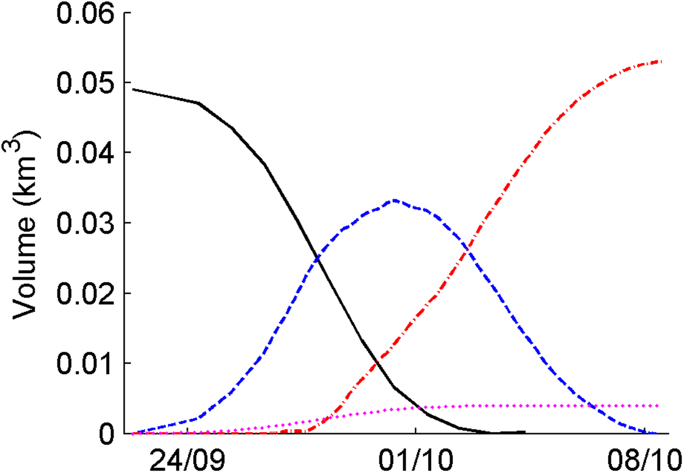
Figure 9 shows the estimated volume of floodwater in the subglacial lake and the cumulative volume of the jökulhlaup discharge at the glacier margin during the September/October 2006 jökulhlaup, as well as the transient volume of water stored in the subglacial pathway. The volume of water in the subglacial pathway is estimated by subtracting the cumulative volume of flood discharge at the terminus from the cumulative volume of floodwater released from the subglacial lake. The subglacial water volume is considerable relative to the total flood volume of 5.3 × 10⁻² km3. It reached a maximum of ~3.3 × 10⁻² km3 on 30 September, 2 days after the outflow from the lake reached its maximum, and was already  $\sim \!\! 1.4 \times 10^{ - 2}\,{\rm k}{\rm m}^3$ before any outflow started at the glacier margin. For flow speed equal to or larger than the mean propagation speed of the subglacial flood front and flood path length of 40 km, one finds that a flood path with a volume of less than half the inferred subglacial water volume is needed to carry the flood discharge at the time of maximum subglacial water storage. This will be elaborated below.
Volume of floodwater in the subglacial lake (solid curve), cumulative volume of the flood discharge at the glacier terminus (dash-dotted curve), the estimated volume of water stored in the subglacial flow path (dashed curve) and calculated amount of melt due to friction in the flow and initial heat of the floodwater (dotted curve). Dates are day/month of 2006.
3.6. Floodwater temperature and thermodynamics
The measurements of floodwater temperature in Skaftá during the September/October 2006 jökulhlaup indicate that the outburst water was within 1°C from the melting point as it emerged from beneath the ice cap. The uncertainty of up to 1°C is caused by frictional heating and heat exchange with the atmosphere along the ~3 km long river path from the terminus to the thermometer location. Measurements of floodwater temperature at the glacier margin in jökulhlaups in Skaftá in August and October 2008 and October 2015 showed floodwater temperatures at the melting point within ± 0.01°C. The measurements were carried out at a discharge close to the maxima of 240 and 1290 m3 s–1 for the August and October jökulhlaups in 2008, respectively, and close to the maximum of ~3000 m3 s–1 for the 2015 jökulhlaup. The predicted outflow temperatures for these events, according to the heat transfer equation in the unsimplified jökulhlaup theory of Nye (Reference Nye1976) as formulated in Jóhannesson (Reference Jóhannesson2002), are 0.05–0.8°C and 1.0–2.5°C for the August and October jökulhlaups in 2008, respectively, and 1.8–3.4°C for the 2015 jökulhlaup. These calculations are based on the geometry of the flood path and channel roughness n m (Manning's roughness) in the range 0.01–0.1 s m–1/3, and also account for the initial heat stored in the lake water.
The vertical temperature profile through the 100 m deep subglacial lake in June 2006 (Jóhannesson and others, 2007) showed that the bulk of the water was close to 4.7°C, with a distinct ~10 m deep layer at 3.5°C at the bottom (both temperatures are higher than the temperature corresponding to maximum density of water at the pressures encountered in the lake). Temperature measurements at different depths in the subglacial lake below the eastern Skaftá cauldron over several months in 2007 showed little variation with time in the lake water temperature, which was close to 4.0°C at most depths (unpublished data from the Icelandic Meteorological Office). The lake water temperature in the western cauldron during the September/October 2006 jökulhlaup may thus be assumed to have been close to 4.5°C.
Most of the initial heat in the lake water is presumably lost during the first few kilometres of the flood path. This is indicated by the few hundred metres wide and up to ~10 m deep depression that stretches ~3 km southwestward from the western cauldron, along the assumed location of the flood path, that is more prominent shortly after jökulhlaups than shortly before the floods, as described above (Figs 1b and 8). The volume change of the depression between the 1998 DEM and the 2010 DEM is  $\sim 1 \cdot 10^{ - 2}\,{\rm k}{\rm m}^3$. Bearing in mind that the heat transfer in subglacial water flow may be assumed to be very rapid (Jóhannesson, Reference Jóhannesson2002; Jarosch and Zwinger, Reference Jarosch and Zwinger2015) and comparing this to the volume of ice melted by the heat content in 0.190 km3 of 4.5°C warm water discharged out of the cauldron in the 2010 jökulhlaup, which is 1.2 × 10⁻² km3, it seems likely that most of the initial heat in the 2010 jökulhlaup floodwater was lost in the flow along this part of the path. These numbers should of course be considered to represent order of magnitudes estimates as the volume of the depression is determined from measurements of the glacier separated by many jökulhlaup cycles. We expected similar heat loss to have taken place in the 2006 jökulhlaup, and therefore the floodwater may be assumed to have been near the melting point for most of the length of the flood path.
4. DISCUSSION AND CONCLUSIONS
Our measurements of the lowering of the ice shelf in the western Skaftá cauldron during a jökulhlaup, along with discharge measurements of the proglacial flood discharge in Skaftá river, allow estimation of the transient subglacial storage of floodwater. The inferred subglacial storage and the measured discharge, along with information on floodwater temperatures in the subglacial reservoir and close to the glacier margin, may be used to draw conclusions about the formation of the subglacial flood path.
At the time of maximum subglacial storage, 4.3 × 10⁻² km3 of water had been released from the subglacial lake (Fig. 9). The initial heat contained in this volume of water with a temperature of ~4.5°C and heat formed by potential energy dissipation in the flow down the subglacial flood path (corresponding to a temperature rise of ~2.0°C) are sufficient to melt at most  $\sim\!\! 3.4 \times 10^{ - 3}\,{\rm k}{\rm m}^3$ of ice (Eqn (3)), if all available thermal energy is used in melting, and considering the potential energy corresponding to the entire elevation difference from the lake to the snout. This is <~10% of the volume of water in the subglacial pathway and subglacial storage along the path, which thus must have been formed mainly by mechanical processes. The ratio of the volume of ice that could have been melted at any particular point in time during the entire rising phase of the jökulhlaup to the subglacial water volume at the same time is also on the order of 10%. Melting therefore cannot have been the main process responsible for the formation of the initial subglacial flood path. Other processes, such as lifting of the ice, hydraulic fracturing as well as viscous and elastic deformation induced by water pressure higher than overburden pressure, must therefore be the main processes responsible for the propagation of the initial jökulhlaup flood wave and the formation of the subglacial path. This is in agreement with earlier findings of Björnsson (Reference Björnsson1992, Reference Björnsson2002), Jóhannesson (Reference Jóhannesson2002), Flowers and others (Reference Flowers, Björnsson, Pálsson and Clarke2004) and Einarsson and others (Reference Einarsson2016) for rapidly rising jökulhlaups, and is in contrast to classic jökulhlaup theory (Nye, Reference Nye1976) where the flood path is formed by a feedback mechanism between water flow and conduit enlargement. Similar transient water storage created by high subglacial water pressure and glacier lifting has been observed for other rapidly rising jökulhlaups at Gornersee, Switzerland (Huss and others, Reference Huss, Bauder, Werder, Funk and Hock2007; Werder and others, Reference Werder, Loye and Funk2009), and at Hidden Creek Lake, Alaska (Bartholomaus and others, Reference Bartholomaus, Anderson and Anderson2008, Reference Bartholomaus, Anderson and Anderson2011). The substantial volume of floodwater that spreads subglacially during the initial phase of the jökulhlaup, $\sim 1.4 \times 10^{ - 2}\,{\rm k}{\rm m}^3$, before any outflow has started at the terminus, also shows that outflow from the subglacial lake does not require direct throughflow of water extending from the lake to the terminus.
It may be assumed that essentially all the subglacial volume of the jökulhlaup path is formed during each individual flood. Preexisting channels, incised into the bedrock or conduits in the ice formed in prior jökulhlaups must be ice-filled since air- or water-filled subglacial cavities in the form of an incipient flood path with a substantial extension are unlikely to be sustained under the glacier between jökulhlaups. According to Nye's (Reference Nye1953) analysis of the contraction of a subglacial cylindrical cavity with the creep parameter for temperate ice from Cuffey and Paterson (Reference Cuffey and Paterson2010), the radius of an air-filled cavity under 400 m of ice will decrease to <10% of its initial value in less than a week. Low and broad air-filled cavities collapse even faster. Water-filled conduits with flowing water will contract and adjust to available water sources between jökulhlaups. This adjustment is not instantaneous but will take place over days to weeks, depending on the position within the glacier and the amplitude and rate of change of water input (Cuffey and Paterson, Reference Cuffey and Paterson2010). Finally, a substantial water body of stagnant water at the glacier bed is only stable in local depressions in the hydraulic potential (Björnsson, Reference Björnsson1988), such as at the cauldrons between jökulhlaups, and such conditions are not present along the flood path of the Skaftá jökulhlaups (Magnússon, Reference Magnússon2003).
Due to the strength of the overlying glacier, the part of the flood path that is initially formed by mechanical processes can be expected to be broad and flat and therefore the flow there will be in the form of a sheet. This part of the path is formed by lifting of the ice through elastic and viscous deformation and hydraulic fracturing induced by water pressure higher than the ice overburden pressure. It is, therefore, unlikely to have a horizontal width smaller than a few ice thicknesses.
Measurements of floodwater temperatures in Skaftá for discharges on the order of 240–3000 m3 s–1 show that the jökulhlaup water is at or very close to the melting point when it emerges at the glacier terminus. Essentially all initial heat of the lake water and heat formed in the flood path by dissipation of potential energy has thus been lost from the floodwater. As pointed out by Björnsson (Reference Björnsson1992), Jóhannesson (Reference Jóhannesson2002) and Clarke (Reference Clarke2003), this indicates much more effective heat transport from the floodwater to the surrounding ice walls of the subglacial flood path than is consistent with the heat transfer mechanism assumed in the classic unsimplified jökulhlaup theory of Nye (Reference Nye1976), and later developments of this theory by Spring and Hutter (Reference Spring and Hutter1981, Reference Spring and Hutter1982) and Fowler (Reference Fowler1999). A better physical understanding of subglacial water flow is clearly needed to explain this very efficient heat transfer (Jóhannesson, Reference Jóhannesson2002; Werder and Funk, Reference Werder and Funk2009; Jarosch and Zwinger, Reference Jarosch and Zwinger2015).
Magnússon and others (Reference Magnússon, Rott, Björnsson and Pálsson2007) observed an increase in surface speed in an 8 km wide area on Skaftárjökull for a small jökulhlaup from the eastern cauldron in 1995, except for the uppermost 6 km of the flood path near the cauldron where no speed-up was observed. They suggested that the 1995 jökulhlaup was drained in a conduit along this uppermost part of the flood path and as a sheet farther down in agreement with the interpretation presented here for the 2006 jökulhlaup. Narrow flood paths with width <500 m extending from both cauldrons are indeed indicated by the elongated surface depressions near the cauldrons described earlier. Although melting driven by the initial heat of the floodwater can only create ~10% of the subglacial water storage, this melting can play an important role over a limited part of the flood path length. A plausible mechanism for the initiation of the flood therefore appears to be (i) melting of a conduit along the first ~3 km of the path, driven by rapid release of the initial heat of the lake water, and (ii) formation of a sheet-like flood path farther down-glacier by lifting and ice deformation due to a propagating subglacial pressure wave (Jóhannesson, Reference Jóhannesson2002; Einarsson and others, Reference Einarsson2016). Such a sheet-like initial subglacial flood path can rapidly develop conduits to become a highly efficient waterway (Jóhannesson, Reference Jóhannesson2002; Flowers and others, Reference Flowers, Björnsson, Pálsson and Clarke2004; Einarsson and others, Reference Einarsson2016) allowing faster rise of discharge than the conduit-melt–discharge feedback (Nye, Reference Nye1976) (Fig. 6, solid curve). The formation of a pressure wave requires an efficient pressure connection between two locations of the flood path where subglacial water pressure near ice overburden at the upper location leads to pressure higher than ice overburden at the (lower) location farther down the path. In the case of the Skaftá cauldrons, the conduit formed by the release of the initial heat near the cauldron may provide this connection with a small potential gradient needed to drive the water flow. This situation may be an essential component in the formation of a subglacial pressure wave in jökulhlaups at this location. The propagating pressure wave would then not be formed at the source lake but some kilometres downstream of it, explaining the shift from conduit flow to sheet flow inferred for the 1995 jökulhlaup by Magnússon and others (Reference Magnússon, Rott, Björnsson and Pálsson2007).
We find that only part of the subglacial water storage is needed to carry the discharge of the flood, even for low estimates of the flow speed, particularly during the initial rise of the flood discharge. This may be interpreted as initial storage in subglacial reservoirs that do not contribute much to the transportation of floodwater. Such transient subglacial storage of floodwater has been documented for a rapidly rising jökulhlaup in 2004 from Gornersee in Switzerland (Huss and others, Reference Huss, Bauder, Werder, Funk and Hock2007; Werder and others, Reference Werder and Funk2009). Up to half of the volume of this flood is reported to have been stored subglacially and they suggest that this storage is related to lateral spreading of the floodwater and uplift of the glacier. This is not a unique feature of rapidly rising jökulhlaups, as lateral spreading and glacier uplift has also been observed for slowly rising jökulhlaups from Grímsvötn and Gornersee, where a propagating subglacial pressure wave was not observed (Huss and others, Reference Huss, Bauder, Werder, Funk and Hock2007; Magnússon and others, Reference Magnússon, Rott, Björnsson and Pálsson2007; Werder and others, Reference Werder, Loye and Funk2009; Magnússon and others, Reference Magnússon2011; Einarsson and others, Reference Einarsson2016).
A rise in the ratio of subglacial volume needed to carry the discharge of the flood to the total volume of subglacial water may be inferred from our data. This indicates a development towards more efficient subglacial water flow and/or release of water from subglacial storage to the main flood path over the course of the 2006 jökulhlaup. This may be interpreted as a development towards effective conduit flow from ineffective initial sheet flow formed in the wake of a subglacial pressure wave.
Our estimate for the travel speed of the subglacial flood front in 2006 (0.2–0.4 m s–1) is faster than the propagation speed of a small jökulhlaup from the eastern Skaftá cauldron in October 1995 (<0.06 m s–1) estimated by Magnússon and others (2007, there is a typo in Magnússon's paper where this speed is given as 0.6 m s–1). Magnússon and others’ (Reference Magnússon, Rott, Björnsson and Pálsson2007) estimation is based on detection of ice surface speed-up due to the jökulhlaup by SAR satellite imagery before the flood front reached the ice margin. Similar propagation speeds as our estimate for the 2006 jökulhlaup have also been estimated for a small jökulhlaup from the western cauldron in August 2008 and a large jökulhlaup from the eastern cauldron in October 2008, 0.1–0.3 and 0.4–0.6 m s–1, respectively (Einarsson and others, Reference Einarsson2016). These travel speed estimates are considerably slower than the speed of the flood front of the rapidly rising jökulhlaup from Grímsvötn in November 1996 (1.3 m s–1) (Björnsson, Reference Björnsson2002) but similar to the speed of a flood front of a rapidly rising jökulhlaup from Hidden Creek Lake, Alaska, in July 2006 (0.4 m s–1) (Bartholomaus and others, Reference Bartholomaus, Anderson and Anderson2011). The speed of the subglacial flood front for rapidly rising jökulhlaups therefore seems to vary between different locations due to differences in flood path geometry, and large subglacial floods appear to propagate faster than small floods at the same location.
There are indications that the speed of the subglacial water flow increases at later stages for jökulhlaups in Skaftá after the proglacial discharge has peaked. This development may also be interpreted as filling of lateral storage of floodwater during the initial phase of the flood that may later release subglacially stored water into the main flood path. Earthquake tremors, indicating boiling within the geothermal system below the subglacial lake, due to the pressure release accompanying the emptying of the lake, were observed during a jökulhlaup from the eastern cauldron in 2002. A time series for the concentration of suspended material in the jökulhlaup waters at the gauging station at Sveinstindur displayed a peak believed to result from the same boiling event. The timing of the earthquake tremors and the peak in the suspended sediments were used to estimate a speed for the subglacial water flow, ~0.8 ± 0.1 m s–1 (O. Sigurðsson, personal communication, 2008). This is 2–4 times the speed estimated here for the initial phase of the 2006 jökulhlaup and 1.3–2 times the speed estimated for the 2008 October jökulhlaup.
The derived shape of the lake at a full stage (Fig. 8) resembles the theoretically predicted shape of subglacial lakes below a surface cauldron with a slope of the ice/water interface at the top of the lake that is opposite to the slope of the ice surface and an order of magnitude larger (Björnsson, Reference Björnsson1975, Reference Björnsson2002). The derived shape does not reflect the full depth and extent of the water body, as some water was left in the lake after the jökulhlaups in 2006 and 2010. For similar ice-shelf thickness in 2010 to that in 2006, ~40 m of water would have been left at the cauldron centre. The resolution of bedrock data is insufficient to determine whether this water is located in a bedrock depression or retained by the closing of the lake seal. The decline of the discharge after the flood peaks varies between jökulhlaups, and the final elevation of the ice shelf after jökulhlaups varies by tens of metres (unpublished data from the Icelandic Meteorological Office and the Institute of Earth Sciences at the University of Iceland). This indicates that the closing of the seal depends delicately on some (subglacial) conditions that vary from event to event. Termination of jökulhlaups before the water level drops below the bedrock threshold is also observed at Grímsvötn (Björnsson, Reference Björnsson1974) and has been assumed to be caused by conduit closing because of ice deformation exceeding melting of conduit walls (Björnsson, Reference Björnsson1974; Nye, Reference Nye1976) or settling of a flat-based ice dam onto a smooth bedrock (Björnsson, Reference Björnsson1974). Some jökulhlaups, for example at Gornersee, continue, however, until the source lake is empty (Werder and others, 2009).
The hypsometric curve for a subglacial lake during lowering in a jökulhlaup depends on the strength of the overlying ice shelf, which determines to what extent the shelf is carried by floating or shear forces. Our simulations show that the shelf has considerable shear strength, due to shear stresses induced by the subsidence that are caused by vertical shear straining over the entire shelf except at the centre, and the local force balance therefore deviates from floating equilibrium. The resulting hypsometric curve is nearly linear (Fig. 5) and not concave as it would be for a lake under an ice shelf mainly carried by floating. Our results show that ice-surface depressions caused by the emptying of subglacial lakes are considerably larger than the footprint of the corresponding water body at the glacier bed; in the case of the western Skaftá cauldron, modelled ice-surface subsidence >1 m is found over an area more than twice that of the subglacial lake. This result may be relevant for time-varying subglacial water bodies at other locations.
Our magnitude for the pressure difference and lateral shear stress, 0.2–0.4 and 0.15–0.3 MPa, respectively, may be crudely compared with the analytical results of the cauldron subsidence model of Evatt and Fowler (Reference Evatt and Fowler2007). Their model predicts ~0.15 and ~0.2 MPa for the pressure difference and shear stress, respectively, when the model parameters have been adapted to the spatial scale of the western Skaftá cauldron, assuming ice flow parameters for temperate ice and a similar outflow magnitude as for the 2006 jökulhlaup. The model of Evatt and Fowler is based on 2-D geometry, rather than cylindrical geometry, and the water outflow is calculated by Nye's (Reference Nye1976) theory for slowly rising jökulhlaups, whereas we employ an outflow variation corresponding to a rapidly rising flood. Considering these differences in assumptions and the formulation of the models, there is overall agreement between the models on the dynamics of the cauldron subsidence.
Many of the most well-known rapidly rising jökulhlaups, such as the jökulhlaups from the Katla volcano (Tómasson, Reference Tómasson1996) and the 1996 Grímsvötn jökulhlaup, are dramatic and up to more than three orders of magnitude larger than the jökulhlaup described in this paper. The relatively small size of the rapidly rising jökulhlaups from the Skaftá cauldrons therefore indicates that the total water volume (i.e. flood size) is not the key factor determining the rapidity of flood release. Considering that some large and small jökulhlaups in Iceland in modern times were rapidly rising (Björnsson, Reference Björnsson2002; Jóhannesson, Reference Jóhannesson2002; Sigurðsson and Einarsson, Reference Sigurðsson and Einarsson2005; Einarsson and others, Reference Einarsson2016), the type of large jökulhlaups at the end of the last glaciation in Iceland and elsewhere must be considered an open question. A fundamental understanding of the conditions that determine the development of subglacial floods, in particular whether they develop rapidly by lifting of the overlying ice or over a longer time through a feedback between discharge and ice melting in a conduit, is therefore required for an improved understanding of prehistoric jökulhlaups. Theoretical studies of the palaeohydraulics of jökulhlaups from Lake Missoula, Montana, USA (Clarke and others, Reference Clarke, Mathews and Pack1984), and Lake Agassiz, North America (Clarke and others, Reference Clarke, Leverington, Teller and Dyke2004), are based on the assumption that these floods were of the slowly rising type and controlled by the melt-discharge-feedback in a conduit. The possibility of a sheet-like flood from Lake Agassiz is deemed highly unlikely by Clarke and others (Reference Clarke, Leverington, Teller, Dyke and Marshall2005) as the inflow into the lake was not rapid and as it is not likely that the critical conditions for ice-dam lifting would be reached over large areas of a dam resting on an irregular bed and variously attacked by iceberg calving. Our example of a rapidly rising flood with an initial sheet-like flood path from the slowly filling subglacial lake below the western Skaftá cauldron shows that rapid inflow is not an essential condition for the release of such floods. Our interpretation also indicates that a flood path that starts as a conduit near the source lake can develop as a sheet farther downstream if a propagating subglacial pressure wave is formed.
ACKNOWLEDGEMENTS
The Icelandic Research Fund, the Landsvirkjun (National Power Company of Iceland) Research Fund, the Icelandic Road Administration, the Kvískerja fund and the Iceland Glaciological Society provided financial and field support, which made this study possible. A map of the subglacial topography along the route of jökulhlaups from the Skaftá cauldrons and the inferred paths of the jökulhlaups shown in Figure 1 was made available by Helgi Björnsson and Finnur Pálsson at the Institute of Earth Sciences of the University of Iceland. Halldór Geirsson at the Icelandic Meteorological Office provided GPS base data from Grímsvötn and Skrokkalda. We thank Olivier Gagliardini for assistance with the Elmer/Ice model calculations. The Icelandic Coast Guard provided helicopter transportation to the western cauldron in November 2006. This material is based upon work supported in part by the National Aeronautics and Space Administration through the NASA Astrobiology Institute under Cooperative Agreement NNA04CC08A issued through the Office of Space Science. Thomas Zwinger was supported by the Nordic Centre of Excellence, ‘eScience Tools for Investigating Climate Change at High Northern Latitudes’ (eSTICC) funded by NordForsk. We thank Vilhjálmur S. Kjartansson, Gunnar Sigurðsson, Hlynur Skagfjörð Pálsson and Mary Miller for assistance during field operations. We thank Gwenn Flowers and two anonymous reviewers of an earlier version of the manuscript and Geoffrey W. Evatt and an anonymous reviewer of this manuscript for detailed and constructive comments that helped us improve the paper and Ken Moxham for help with the English language. This publication is contribution No. 4 of the Nordic Centre of Excellence SVALI, ‘Stability and Variations of Arctic Land Ice’, funded by the Nordic Top-level Research Initiative (TRI).


 Open access