


1 Introduction
The theory of hyperplane arrangements is a bridge between geometry, algebra and combinatorics, with countless applications across these fields and other areas of mathematics. The leitmotif of arrangement theory consists in the explicit computation of geometric invariants – such as cohomology and homotopy type – from combinatorial data associated with the arrangement, such as the poset of layers or the poset of faces. Foundational results of this kind have been discovered for several decades: the Orlik-Solomon algebra [Reference Arnol’ d1, Reference Orlik and Solomon28], the Salvetti complex [Reference Salvetti34], the cohomology of wonderful models of hyperplane arrangements [Reference Concini and Procesi11, Reference Feichtner and Yuzvinsky19], among others.
In the last two decades, the researchers’ attention has shifted toward more general types of arrangements, where the ambient vector space is replaced with richer and more interesting topological spaces. Motivated by applications to integral polytopes and box-splines, De Concini and Procesi [Reference Concini and Procesi12, Reference Concini and Procesi13] initiated the study of toric arrangements, defined as collections of hypertori in a complex torus. More recently, other generalizations have emerged: elliptic arrangements, which are collections of a certain type of divisors in a product of elliptic curves $\mathcal {E}^n$
, and abelian arrangements, defined as collections of certain subgroups in an ambient space
$\mathcal {E}^n$
, and abelian arrangements, defined as collections of certain subgroups in an ambient space $G^n$
where G is an abelian Lie group.
$G^n$
where G is an abelian Lie group.
The connection between topological invariants and combinatorics persists for toric arrangements, although in a subtler way [Reference Moci26, Reference D’Adderio and Moci9, Reference d’Antonio and Delucchi10, Reference Callegaro and Delucchi8, Reference Callegaro, D’Adderio, Delucchi, Migliorini and Pagaria7, Reference Moci and Pagaria27], [Reference Pagaria30], while it becomes weaker in the elliptic case [Reference Levin and Varchenko24, Reference Delucchi and Pagaria15] [Reference Pagaria31] and in the abelian case [Reference Bibby3, Reference Tran and Yoshinaga37, Reference Liu, Nhat Tran and Yoshinaga25, Reference Bibby and Delucchi4, Reference Bazzocchi, Pagaria and Pismataro2].
The standard definition of elliptic arrangements, used in the literature, is independent of the specific elliptic curve $\mathcal {E}$
. In fact, one only considers divisors in
$\mathcal {E}$
. In fact, one only considers divisors in $\mathcal {E}^n$
of the form
$\mathcal {E}^n$
of the form $\ker \phi $
where
$\ker \phi $
where
with $m_i \in \mathbb {Z}$
. In fact, in this framework the elliptic curve is treated as a topological group
$m_i \in \mathbb {Z}$
. In fact, in this framework the elliptic curve is treated as a topological group $\mathcal {E} \simeq S^1 \times S^1$
that admits an Hodge structure.
$\mathcal {E} \simeq S^1 \times S^1$
that admits an Hodge structure.
In this work, we provide a more general and natural definition of an elliptic arrangement, which is also sensitive to the choice of the curve $\mathcal {E}$
, thereby introducing number-theoretic aspects into the picture.
$\mathcal {E}$
, thereby introducing number-theoretic aspects into the picture.
More precisely, let us recall that every endomorphism of an elliptic curve $\mathcal {E}$
arises from multiplication by a complex number lying in a subring
$\mathcal {E}$
arises from multiplication by a complex number lying in a subring $R_{\mathcal {E}}$
of a quadratic number field. The ring of integers
$R_{\mathcal {E}}$
of a quadratic number field. The ring of integers ${\mathbb Z}$
is always contained in
${\mathbb Z}$
is always contained in $R_{\mathcal {E}}$
. Generically
$R_{\mathcal {E}}$
. Generically $R_{\mathcal {E}} = {\mathbb Z}$
, but some elliptic curves, called of complex multiplication type (CM), admit more endomorphisms. While all the cited papers assume that
$R_{\mathcal {E}} = {\mathbb Z}$
, but some elliptic curves, called of complex multiplication type (CM), admit more endomorphisms. While all the cited papers assume that $m_i \in {\mathbb Z} \subseteq \operatorname {End}(\mathcal {E})$
, in the present paper we drop such assumption, building a more general family of hypersurfaces. In other words, we define elliptic arrangements as collections of kernels of arbitrary morphisms of abelian varieties
$m_i \in {\mathbb Z} \subseteq \operatorname {End}(\mathcal {E})$
, in the present paper we drop such assumption, building a more general family of hypersurfaces. In other words, we define elliptic arrangements as collections of kernels of arbitrary morphisms of abelian varieties $\phi \colon \mathcal {E}^n \to \mathcal {E}$
. We extend all previous results to this setting, which allows us to address new phenomena that arise when
$\phi \colon \mathcal {E}^n \to \mathcal {E}$
. We extend all previous results to this setting, which allows us to address new phenomena that arise when $\mathcal {E}$
has complex multiplication.
$\mathcal {E}$
has complex multiplication.
In Section 2, we recall some basic facts about the endomorphism ring $R_{\mathcal {E}} := \operatorname {End}(\mathcal {E})$
of an elliptic curve
$R_{\mathcal {E}} := \operatorname {End}(\mathcal {E})$
of an elliptic curve $\mathcal {E}$
of complex multiplication type. In particular
$\mathcal {E}$
of complex multiplication type. In particular $R_{\mathcal {E}}$
is an order in a quadratic imaginary number field. In Section 3 we introduce hyperplane, toric, and elliptic arrangements. While the description of the intersections is trivial in the hyperplane case, simple in the toric one, it becomes significantly more complex for the elliptic arrangements. A matrix
$R_{\mathcal {E}}$
is an order in a quadratic imaginary number field. In Section 3 we introduce hyperplane, toric, and elliptic arrangements. While the description of the intersections is trivial in the hyperplane case, simple in the toric one, it becomes significantly more complex for the elliptic arrangements. A matrix $A \in \operatorname {Mat}_{k,n}(R_{\mathcal {E}})$
defines an elliptic arrangement of k divisors in
$A \in \operatorname {Mat}_{k,n}(R_{\mathcal {E}})$
defines an elliptic arrangement of k divisors in $\mathcal {E}^n$
. For any
$\mathcal {E}^n$
. For any $S \subseteq [k]$
, we show that the intersection
$S \subseteq [k]$
, we show that the intersection $\mathcal {A}_S$
of the corresponding divisors fits into a short exact sequence:
$\mathcal {A}_S$
of the corresponding divisors fits into a short exact sequence:
Here, $\pi _S$
denotes the selection of rows of the matrix A indexed by S. In particular, each intersection
$\pi _S$
denotes the selection of rows of the matrix A indexed by S. In particular, each intersection ${\mathcal {A}}_S$
is an extension between an abelian variety and a finite group. Moreover, the number of connected components (or layers) in
${\mathcal {A}}_S$
is an extension between an abelian variety and a finite group. Moreover, the number of connected components (or layers) in ${\mathcal {A}}_S$
equals
${\mathcal {A}}_S$
equals $\# \operatorname {tor} \operatorname {coker} \pi _S \circ A$
(see Lemma 3.1). We also characterize the abelian varieties that can appear as a layer of an elliptic arrangement in
$\# \operatorname {tor} \operatorname {coker} \pi _S \circ A$
(see Lemma 3.1). We also characterize the abelian varieties that can appear as a layer of an elliptic arrangement in $\mathcal {E}^n$
: they are products of elliptic curves
$\mathcal {E}^n$
: they are products of elliptic curves $\mathcal {E}_i$
that are isogenous to
$\mathcal {E}_i$
that are isogenous to $\mathcal {E}$
, with the conductor of
$\mathcal {E}$
, with the conductor of $\operatorname {End}(\mathcal {E}_i)$
dividing that of
$\operatorname {End}(\mathcal {E}_i)$
dividing that of $\operatorname {End}(\mathcal {E})$
(see Lemma 3.3).
$\operatorname {End}(\mathcal {E})$
(see Lemma 3.3).
In Section 4, we study ${\mathcal {A}}_S$
as a
${\mathcal {A}}_S$
as a $R_{\mathcal {E}}$
-module, illustrating through examples how the situation is more subtle than considering
$R_{\mathcal {E}}$
-module, illustrating through examples how the situation is more subtle than considering ${\mathcal {A}}_S$
only as
${\mathcal {A}}_S$
only as ${\mathbb Z}$
-module. In particular, we present Example 4.2 where the short exact sequence (1.1) does not split as
${\mathbb Z}$
-module. In particular, we present Example 4.2 where the short exact sequence (1.1) does not split as $R_{\mathcal {E}}$
-modules, and we completely characterize when it splits (see Proposition 4.6). Furthermore, the matrix A induces maps
$R_{\mathcal {E}}$
-modules, and we completely characterize when it splits (see Proposition 4.6). Furthermore, the matrix A induces maps $A_\Lambda \colon \Lambda ^n \to \Lambda ^k$
and
$A_\Lambda \colon \Lambda ^n \to \Lambda ^k$
and $A_R \colon R^n \to R^k$
and we prove in Lemma 4.11 that
$A_R \colon R^n \to R^k$
and we prove in Lemma 4.11 that
 $$\begin{align*}\Lambda^k / A_\Lambda(\Lambda^n) \cong R^k / A_R( R^n) \end{align*}$$
as ${\mathbb Z}$
-modules, thereby filling a gap in the preprint [Reference Borzì and Martino5] (c.f. Remark 4.12).
${\mathbb Z}$
-modules, thereby filling a gap in the preprint [Reference Borzì and Martino5] (c.f. Remark 4.12).
In Section 5, we recall the notion of arithmetic matroid, introduced in [Reference D’Adderio and Moci9], and show that every elliptic arrangement $\mathcal {A}$
gives rise to such a structure. Specifically, the ground set
$\mathcal {A}$
gives rise to such a structure. Specifically, the ground set $[k]$
, the rank function
$[k]$
, the rank function $\operatorname {rk}_{\mathcal {A}} (S)= \dim _{\mathbb {C}} \ker \pi _S \circ A_{\mathbb {C}}$
, and the multiplicity function
$\operatorname {rk}_{\mathcal {A}} (S)= \dim _{\mathbb {C}} \ker \pi _S \circ A_{\mathbb {C}}$
, and the multiplicity function $m_{\mathcal {A}}(S) = \# \operatorname {tor} \operatorname {coker} \pi _{S} \circ A $
define an arithmetic matroid (Theorem 5.11). The proof relies on a new duality construction for elliptic arrangements (Lemma 5.9). Interestingly, while arithmetic matroids were originally introduced to study toric arrangements, we show an elliptic arrangement that corresponds to a nonrealizable arithmetic matroid (Example 5.13). We also observe that the so-called GCD property holds when
$m_{\mathcal {A}}(S) = \# \operatorname {tor} \operatorname {coker} \pi _{S} \circ A $
define an arithmetic matroid (Theorem 5.11). The proof relies on a new duality construction for elliptic arrangements (Lemma 5.9). Interestingly, while arithmetic matroids were originally introduced to study toric arrangements, we show an elliptic arrangement that corresponds to a nonrealizable arithmetic matroid (Example 5.13). We also observe that the so-called GCD property holds when $R_{\mathcal {E}}$
is Dedekind (Lemma 5.14), but not in general. We briefly relate elliptic arrangements to (poly-)matroids over
$R_{\mathcal {E}}$
is Dedekind (Lemma 5.14), but not in general. We briefly relate elliptic arrangements to (poly-)matroids over $R_{\mathcal {E}}$
, introduced in [Reference Fink and Moci20]. Finally, we compute the Euler characteristic of the complement of an elliptic arrangement (Theorem 5.16), extending Bibby’s work [Reference Bibby3] to the complex multiplication case.
$R_{\mathcal {E}}$
, introduced in [Reference Fink and Moci20]. Finally, we compute the Euler characteristic of the complement of an elliptic arrangement (Theorem 5.16), extending Bibby’s work [Reference Bibby3] to the complex multiplication case.
2 Background on elliptic curves
2.1 Notation
We write $[k]$
for
$[k]$
for $\left \{ 1,2, \dots , k \right \}$
;
$\left \{ 1,2, \dots , k \right \}$
; $\# X$
for cardinality of a set;
$\# X$
for cardinality of a set; $X \cup i$
for
$X \cup i$
for $X \cup \left \{ i \right \}$
; SES for Short Exact Sequence;
$X \cup \left \{ i \right \}$
; SES for Short Exact Sequence; $\operatorname {CC}(X)$
for connected components of X.
$\operatorname {CC}(X)$
for connected components of X.
2.2 Elliptic curves with complex multiplication
Let $\mathcal {E}$
be a smooth complex Riemann surface of genus one. All such
$\mathcal {E}$
be a smooth complex Riemann surface of genus one. All such $\mathcal {E}$
are isomorphic to
$\mathcal {E}$
are isomorphic to ![]() , with
, with $\Lambda $
a lattice generated by
$\Lambda $
a lattice generated by $1$
and
$1$
and $\tau \in {\mathbb C} \setminus {\mathbb R}$
, and group structure induced by
$\tau \in {\mathbb C} \setminus {\mathbb R}$
, and group structure induced by $({\mathbb C}, +)$
. If
$({\mathbb C}, +)$
. If $\operatorname {End}(\mathcal {E}) \ne {\mathbb Z}$
we say that
$\operatorname {End}(\mathcal {E}) \ne {\mathbb Z}$
we say that $\mathcal {E}$
has complex multiplication type. We recall some properties of
$\mathcal {E}$
has complex multiplication type. We recall some properties of $\operatorname {End}(\mathcal {E})$
and
$\operatorname {End}(\mathcal {E})$
and $\Lambda $
; for details and introductory references, see [Reference Silverman35] or [Reference Silverman and Tate36].
$\Lambda $
; for details and introductory references, see [Reference Silverman35] or [Reference Silverman and Tate36].
2.2.1 The endomorphism ring
We describe a ring $R_{\mathcal {E}}$
isomorphic to
$R_{\mathcal {E}}$
isomorphic to $\operatorname {End}(\mathcal {E})$
. Denote by
$\operatorname {End}(\mathcal {E})$
. Denote by $A_\alpha $
the linear map given by multiplication by
$A_\alpha $
the linear map given by multiplication by $\alpha $
, that is,
$\alpha $
, that is, $z \mapsto \alpha z$
.
$z \mapsto \alpha z$
.
Lemma 2.1. For an elliptic curve $\mathcal {E} = {\mathbb C} / \Lambda $
, the ring
$\mathcal {E} = {\mathbb C} / \Lambda $
, the ring $\operatorname {End}(\mathcal {E})$
is isomorphic to
$\operatorname {End}(\mathcal {E})$
is isomorphic to
 $$\begin{align*}R_{\mathcal{E}} = \left\{ \alpha \in \Lambda \colon \, \alpha \Lambda \subset \Lambda \right\}\end{align*}$$
via the map $R_{\mathcal {E}} \to \operatorname {End}(\mathcal {E})$
defined by
$R_{\mathcal {E}} \to \operatorname {End}(\mathcal {E})$
defined by $\alpha \mapsto A_\alpha $
.
$\alpha \mapsto A_\alpha $
.
Sketch of proof.
One shows that if ![]() is an endomorphism, then an analytic continuation
is an endomorphism, then an analytic continuation $\hat f \colon {\mathbb C} \to {\mathbb C}$
of f around 0 is of the form
$\hat f \colon {\mathbb C} \to {\mathbb C}$
of f around 0 is of the form $\hat f(z) = \alpha z$
. Moreover,
$\hat f(z) = \alpha z$
. Moreover, $\alpha $
must have the property that
$\alpha $
must have the property that $\alpha \Lambda \subset \Lambda $
for f being well defined when descending to
$\alpha \Lambda \subset \Lambda $
for f being well defined when descending to ![]() . See Proposition 6.17 of [Reference Silverman and Tate36] for details.
. See Proposition 6.17 of [Reference Silverman and Tate36] for details.
We write R instead of $R_{\mathcal {E}}$
when
$R_{\mathcal {E}}$
when $\mathcal {E}$
is clear from the context.
$\mathcal {E}$
is clear from the context.
2.2.2 A quadratic relation for $\tau $

Assume that $\operatorname {End}(\mathcal {E}) \not \cong {\mathbb Z}$
and consider
$\operatorname {End}(\mathcal {E}) \not \cong {\mathbb Z}$
and consider $\alpha $
in R. By Lemma 2.1 we have
$\alpha $
in R. By Lemma 2.1 we have $\alpha \Lambda \subset \Lambda $
. Equivalently,
$\alpha \Lambda \subset \Lambda $
. Equivalently, $\alpha \cdot 1 \in \Lambda $
and
$\alpha \cdot 1 \in \Lambda $
and $\alpha \cdot \tau \in \Lambda $
. Having
$\alpha \cdot \tau \in \Lambda $
. Having $\alpha \cdot 1 \in \Lambda $
gives
$\alpha \cdot 1 \in \Lambda $
gives $R \subset \Lambda $
, so we can write
$R \subset \Lambda $
, so we can write $\alpha = x + y\tau $
with
$\alpha = x + y\tau $
with $x, y \in {\mathbb Z}$
. Thus,
$x, y \in {\mathbb Z}$
. Thus, $\alpha \cdot \tau = x\tau + y\tau ^2$
. Hence, the second condition
$\alpha \cdot \tau = x\tau + y\tau ^2$
. Hence, the second condition $\alpha \cdot \tau \in \Lambda $
is true if and only if
$\alpha \cdot \tau \in \Lambda $
is true if and only if $y\tau ^2$
is in
$y\tau ^2$
is in $\Lambda $
. That is, for some
$\Lambda $
. That is, for some $h, k \in {\mathbb Z}$
we have
$h, k \in {\mathbb Z}$
we have
 $$ \begin{align} y\tau^2 = h\tau + k. \end{align} $$
Lemma 2.2. If $\mathcal {E} = {\mathbb C} / \langle 1, \tau \rangle $
has
$\mathcal {E} = {\mathbb C} / \langle 1, \tau \rangle $
has $\operatorname {End}(\mathcal {E}) \not \cong {\mathbb Z}$
, then
$\operatorname {End}(\mathcal {E}) \not \cong {\mathbb Z}$
, then ${\mathbb Q}[\tau ]$
is a quadratic imaginary number field and
${\mathbb Q}[\tau ]$
is a quadratic imaginary number field and $R_{\mathcal {E}}$
is an order, that is, a subring of the ring of integers
$R_{\mathcal {E}}$
is an order, that is, a subring of the ring of integers ${{\mathcal {O}}}_{{\mathbb Q}[\tau ]}$
of rank two.
${{\mathcal {O}}}_{{\mathbb Q}[\tau ]}$
of rank two.
Proof. If $y=0$
in Equation (2.1), then
$y=0$
in Equation (2.1), then $\alpha = x$
is an integer. So
$\alpha = x$
is an integer. So $\operatorname {End}(\mathcal {E}) \not \cong {\mathbb Z}$
is equivalent to the existence of a nonzero choice for y, which gives the quadratic relation
$\operatorname {End}(\mathcal {E}) \not \cong {\mathbb Z}$
is equivalent to the existence of a nonzero choice for y, which gives the quadratic relation $y\tau ^2 - h\tau - k = 0$
for
$y\tau ^2 - h\tau - k = 0$
for $\tau $
. Moreover,
$\tau $
. Moreover, $\tau $
is nonreal because otherwise
$\tau $
is nonreal because otherwise $\operatorname {span}_{\mathbb Z} \left \{ 1, \tau \right \}$
would not be a lattice in
$\operatorname {span}_{\mathbb Z} \left \{ 1, \tau \right \}$
would not be a lattice in ${\mathbb C}$
. This proves the statement about
${\mathbb C}$
. This proves the statement about ${\mathbb Q}[\tau ]$
.
${\mathbb Q}[\tau ]$
.
Recall that the ring of integers ${{\mathcal {O}}}$
is the subring of algebraic numbers
${{\mathcal {O}}}$
is the subring of algebraic numbers $\alpha \in {\mathbb Q}[\tau ]$
whose minimal polynomial
$\alpha \in {\mathbb Q}[\tau ]$
whose minimal polynomial $f_\alpha $
over
$f_\alpha $
over ${\mathbb Z}$
is monic. To see that
${\mathbb Z}$
is monic. To see that $\alpha \in R_{\mathcal {E}}$
is an algebraic integer, multiply Equation (2.1) by y to get the monic relation
$\alpha \in R_{\mathcal {E}}$
is an algebraic integer, multiply Equation (2.1) by y to get the monic relation $(y\tau )^2 -h(y\tau ) - yk = 0$
, thus
$(y\tau )^2 -h(y\tau ) - yk = 0$
, thus $y\tau \in {{\mathcal {O}}}$
. Since
$y\tau \in {{\mathcal {O}}}$
. Since $x \in {\mathbb Z}$
, we have that
$x \in {\mathbb Z}$
, we have that $\alpha = x + y\tau $
is in
$\alpha = x + y\tau $
is in ${{\mathcal {O}}}$
as desired.
${{\mathcal {O}}}$
as desired.
2.2.3 Quadratic number fields
In view of Lemma 2.2, we recall that every imaginary quadratic number field can be obtained via a unique choice of a square-free positive integer m: let $K_m = {\mathbb Q}(\sqrt {-m})$
be the field containing
$K_m = {\mathbb Q}(\sqrt {-m})$
be the field containing $\tau $
. Consider
$\tau $
. Consider
 $$ \begin{align} \omega = \begin{cases} \frac{1 + \sqrt{-m}}{2} & \text{ if } m \equiv 3 \quad\mod 4,\\ \sqrt{-m} & \text{ otherwise,} \end{cases} \end{align} $$
and recall that ${{\mathcal {O}}}_m = {\mathbb Z}[\omega ]$
is the ring of integers of
${{\mathcal {O}}}_m = {\mathbb Z}[\omega ]$
is the ring of integers of $K_m$
. In the first case we have the minimal polynomial
$K_m$
. In the first case we have the minimal polynomial $f^{\mathbb Z}_\omega (\omega ) = \omega ^2-\omega +m'= 0$
where
$f^{\mathbb Z}_\omega (\omega ) = \omega ^2-\omega +m'= 0$
where $4m'-1 = m$
, and in the second case
$4m'-1 = m$
, and in the second case $f^{\mathbb Z}_\omega (\omega ) = \omega ^2 +m = 0$
. Since
$f^{\mathbb Z}_\omega (\omega ) = \omega ^2 +m = 0$
. Since $\tau $
is in
$\tau $
is in $K_m$
, we can choose integers
$K_m$
, we can choose integers $a,b,c$
with
$a,b,c$
with $\gcd (a,b,c) = 1$
such that
$\gcd (a,b,c) = 1$
such that $\tau = \frac {a+b\omega }{c} \in K_m$
. Calculate
$\tau = \frac {a+b\omega }{c} \in K_m$
. Calculate
 $$ \begin{align} \operatorname{tr} A_\tau &= \begin{cases} (2a+b)/c & \text{ if } m \equiv 3 \quad\mod 4,\\ 2a/c & \text{ else,} \end{cases} \end{align} $$
 $$ \begin{align} \det A_\tau &=\begin{cases} (a^2 + ab +b^2m')/c^2 & \text{ if } m \equiv 3 \quad\mod 4,\\ (a^2 + b^2m)/c^2 & \text{ else;} \end{cases} \end{align} $$
where $\operatorname {tr} A_\tau $
and
$\operatorname {tr} A_\tau $
and $\det A_\tau $
are the trace and determinant of the linear map
$\det A_\tau $
are the trace and determinant of the linear map $z \mapsto \tau z$
. Thus, the minimal polynomial over
$z \mapsto \tau z$
. Thus, the minimal polynomial over ${\mathbb Q}$
of
${\mathbb Q}$
of $\tau $
is the characteristic polynomial of
$\tau $
is the characteristic polynomial of $A_\tau $
:
$A_\tau $
:
 $$ \begin{align} f^{\mathbb Q}_\tau(\tau) = \tau^2 - \operatorname{tr} A_\tau \tau + \det A_\tau. \end{align} $$
2.2.4 Generators for
$R_{\mathcal {E}}$

Consider the isomorphism $(x, y) \mapsto x \cdot 1 + y \cdot \tau $
between
$(x, y) \mapsto x \cdot 1 + y \cdot \tau $
between ${\mathbb Z}^2$
and
${\mathbb Z}^2$
and $\Lambda $
. Since R is a subgroup of
$\Lambda $
. Since R is a subgroup of $\Lambda \cong {\mathbb Z}^2$
with
$\Lambda \cong {\mathbb Z}^2$
with $1 \in R$
, we conclude that R is equal to
$1 \in R$
, we conclude that R is equal to $\langle 1, N \tau \rangle $
for some nonzero integer N. As a consequence of Equation (2.5) and the fact that
$\langle 1, N \tau \rangle $
for some nonzero integer N. As a consequence of Equation (2.5) and the fact that $N\tau ^2$
must have integral coordinates in the basis
$N\tau ^2$
must have integral coordinates in the basis $\left \{ 1, \tau \right \}$
we get that:
$\left \{ 1, \tau \right \}$
we get that:
Lemma 2.3. We have that $R = \langle 1, N \tau \rangle $
if and only if
$R = \langle 1, N \tau \rangle $
if and only if $N f^{\mathbb Q}_\tau $
equals the primitive minimal polynomial
$N f^{\mathbb Q}_\tau $
equals the primitive minimal polynomial $f^{\mathbb Z}_\tau $
of
$f^{\mathbb Z}_\tau $
of $\tau $
over
$\tau $
over ${\mathbb Z}$
.
${\mathbb Z}$
.
We assume that N is positive, and calculate:
Lemma 2.4. We have that
 $$\begin{align*}N = c^2/\gcd(c, c^2\det A_\tau). \end{align*}$$
Proof. This follows from clearing up denominators from $\operatorname {tr} A_\tau $
and
$\operatorname {tr} A_\tau $
and $\det A_\tau $
in Equation (2.5). The equalities
$\det A_\tau $
in Equation (2.5). The equalities
 $$ \begin{align*} \gcd(c^2, (2a+b)c, a^2+ab+b^2m') &= \gcd(c, a^2+ab+b^2m') & & \text{ if } m\equiv 3 \quad\mod 4, \\ \gcd(c^2, 2ac, a^2+b^2m) &= \gcd(c, a^2+b^2m) && \text{ otherwise}; \end{align*} $$
hold by the hypothesis $\gcd (a,b,c)=1$
and the claimed result follows.
$\gcd (a,b,c)=1$
and the claimed result follows.
Remark 2.5. An order in a number field K is a subring whose additive group is finitely generated of rank equal to $[K:\mathbb Q]$
. Thus,
$[K:\mathbb Q]$
. Thus, $R_{\mathcal {E}}$
is an order in
$R_{\mathcal {E}}$
is an order in $K_m$
.
$K_m$
.
3 Arrangements
A central abelian arrangement ${\mathcal {A}}$
is a collection of codimension-1 Lie subgroups
${\mathcal {A}}$
is a collection of codimension-1 Lie subgroups $H_1, \dots , H_k$
in
$H_1, \dots , H_k$
in $G^n$
where G is an abelian Lie group. The subgroups
$G^n$
where G is an abelian Lie group. The subgroups $H_i$
are of the form
$H_i$
are of the form $\ker \phi _i$
for some
$\ker \phi _i$
for some $\phi _i \in \operatorname {\mathrm {Hom}} (G^n,G)$
. Let
$\phi _i \in \operatorname {\mathrm {Hom}} (G^n,G)$
. Let $\operatorname {CM}({\mathcal {A}}) = G^n \setminus \bigcup _{i \in [k]} H_i $
be the complement; the study of the topology of
$\operatorname {CM}({\mathcal {A}}) = G^n \setminus \bigcup _{i \in [k]} H_i $
be the complement; the study of the topology of $\operatorname {CM}({\mathcal {A}})$
is one of the motivations to study
$\operatorname {CM}({\mathcal {A}})$
is one of the motivations to study ${\mathcal {A}}$
. We recall the affine and toric cases, to motivate our elliptic setting.
${\mathcal {A}}$
. We recall the affine and toric cases, to motivate our elliptic setting.
3.1 Abelian arrangements
3.1.1 Hyperplane arrangements
Here $G = (K,+)$
for some field K and
$G = (K,+)$
for some field K and $\phi _i$
is some functional in
$\phi _i$
is some functional in $\operatorname {\mathrm {Hom}}(K^n, K)$
, thus
$\operatorname {\mathrm {Hom}}(K^n, K)$
, thus $H_i$
is a hyperplane. A result by Orlik and Solomon establishes that an important combinatorial invariant of
$H_i$
is a hyperplane. A result by Orlik and Solomon establishes that an important combinatorial invariant of ${\mathcal {A}}$
is the lattice of intersections
${\mathcal {A}}$
is the lattice of intersections ${{\mathcal {P}}}({\mathcal {A}})$
, that is, affine spaces
${{\mathcal {P}}}({\mathcal {A}})$
, that is, affine spaces $\left \{ \bigcap _{i \in S} H_i \colon \, S \subset [k] \right \}$
partially ordered by reverse inclusion. From
$\left \{ \bigcap _{i \in S} H_i \colon \, S \subset [k] \right \}$
partially ordered by reverse inclusion. From ${{\mathcal {P}}}({\mathcal {A}})$
one can reconstruct some topological data of the complement
${{\mathcal {P}}}({\mathcal {A}})$
one can reconstruct some topological data of the complement $\operatorname {CM}({\mathcal {A}})$
: cohomology when
$\operatorname {CM}({\mathcal {A}})$
: cohomology when $K = \mathbb C$
, number of connected components when
$K = \mathbb C$
, number of connected components when $K = {\mathbb R}$
, number of points when K is a finite field
$K = {\mathbb R}$
, number of points when K is a finite field ${\mathbb F}_q$
. See [Reference Dimca17, Theorem 3.5] for an introduction.
${\mathbb F}_q$
. See [Reference Dimca17, Theorem 3.5] for an introduction.
It turns out that ${{\mathcal {P}}}({\mathcal {A}})$
as a lattice is semimodular and atomic, thus cryptomorphically is a matroid, realizable over K, on the groundset
${{\mathcal {P}}}({\mathcal {A}})$
as a lattice is semimodular and atomic, thus cryptomorphically is a matroid, realizable over K, on the groundset $[k]$
; see [Reference Oxley29, Section 1.7]. Our philosophy is to generalize the matroid approach.
$[k]$
; see [Reference Oxley29, Section 1.7]. Our philosophy is to generalize the matroid approach.
3.1.2 Toric arrangements
Here $G = ({\mathbb C}^*,*)$
is the multiplicative group and
$G = ({\mathbb C}^*,*)$
is the multiplicative group and $\phi _i$
is some character in
$\phi _i$
is some character in $\operatorname {\mathrm {Hom}}(({\mathbb C}^*)^n, {\mathbb C}^*)\simeq {\mathbb Z}^n$
, so
$\operatorname {\mathrm {Hom}}(({\mathbb C}^*)^n, {\mathbb C}^*)\simeq {\mathbb Z}^n$
, so $H_i$
is a union of subtori of codimension 1. We will not consider here the case of subtori of arbitrary codimension, which has been studied in [Reference Moci and Pagaria27]. Write
$H_i$
is a union of subtori of codimension 1. We will not consider here the case of subtori of arbitrary codimension, which has been studied in [Reference Moci and Pagaria27]. Write ${\mathcal {A}}_S$
for the intersection
${\mathcal {A}}_S$
for the intersection $\bigcap _{i \in S} H_i$
for some
$\bigcap _{i \in S} H_i$
for some $S \subset [k]$
. In the toric and elliptic cases
$S \subset [k]$
. In the toric and elliptic cases ${\mathcal {A}}_S$
is generally not connected. We call an element of
${\mathcal {A}}_S$
is generally not connected. We call an element of $\operatorname {CC}({\mathcal {A}}_S)$
a layer, that is, a connected component of
$\operatorname {CC}({\mathcal {A}}_S)$
a layer, that is, a connected component of ${\mathcal {A}}_S$
. All layers of
${\mathcal {A}}_S$
. All layers of $\operatorname {CC}({\mathcal {A}}_S)$
have the same dimension. If
$\operatorname {CC}({\mathcal {A}}_S)$
have the same dimension. If $\ell _1$
and
$\ell _1$
and $\ell _2$
are layers such that
$\ell _2$
are layers such that $\# \operatorname {CC}(\ell _1 \cap \ell _2) \ge 2$
, there is no unique minimal upper bound of
$\# \operatorname {CC}(\ell _1 \cap \ell _2) \ge 2$
, there is no unique minimal upper bound of $\ell _1$
and
$\ell _1$
and $\ell _2$
in the poset
$\ell _2$
in the poset $\left \{ \bigcap _{i \in S} H_i \colon \, S \subset [k] \right \}$
, so we do not have a lattice. Thus, we call
$\left \{ \bigcap _{i \in S} H_i \colon \, S \subset [k] \right \}$
, so we do not have a lattice. Thus, we call ${{\mathcal {C}}}({\mathcal {A}})$
the poset of layers.
${{\mathcal {C}}}({\mathcal {A}})$
the poset of layers.
This also means that ${{\mathcal {C}}}({\mathcal {A}})$
cannot correspond to a matroid. This is partially fixed in [Reference Moci26] by considering the triple
${{\mathcal {C}}}({\mathcal {A}})$
cannot correspond to a matroid. This is partially fixed in [Reference Moci26] by considering the triple $([k], \operatorname {rk}, m)$
of the functions
$([k], \operatorname {rk}, m)$
of the functions $\operatorname {rk} S = \operatorname {codim} A_S$
and
$\operatorname {rk} S = \operatorname {codim} A_S$
and $m(S) = \# \operatorname {CC}({\mathcal {A}}_S)$
. These satisfy some axioms that are christened an arithmetic matroid in [Reference D’Adderio and Moci9, Reference Brändén and Moci6]. The arithmetic matroid contains enough information to define an arithmetic Tutte polynomial that, like in the hyperplane case, yields important invariants as evaluations [Reference Moci26]. For example: the Poincare polynomial, whose coefficients encode the Betti numbers of the complement
$m(S) = \# \operatorname {CC}({\mathcal {A}}_S)$
. These satisfy some axioms that are christened an arithmetic matroid in [Reference D’Adderio and Moci9, Reference Brändén and Moci6]. The arithmetic matroid contains enough information to define an arithmetic Tutte polynomial that, like in the hyperplane case, yields important invariants as evaluations [Reference Moci26]. For example: the Poincare polynomial, whose coefficients encode the Betti numbers of the complement $\operatorname {CM}({\mathcal {A}})$
; the characteristic polynomial of
$\operatorname {CM}({\mathcal {A}})$
; the characteristic polynomial of ${{\mathcal {C}}}({\mathcal {A}})$
, associated with any poset and containing homological information of its order complex.
${{\mathcal {C}}}({\mathcal {A}})$
, associated with any poset and containing homological information of its order complex.
3.1.3 Elliptic arrangements
Here $G = \mathcal {E}$
for some elliptic curve
$G = \mathcal {E}$
for some elliptic curve $\mathcal {E} = {\mathbb C} / \Lambda $
and
$\mathcal {E} = {\mathbb C} / \Lambda $
and $\phi _i$
is in
$\phi _i$
is in $\operatorname {\mathrm {Hom}}(\mathcal {E}^n, \mathcal {E})$
. By Section 2.2 we regard
$\operatorname {\mathrm {Hom}}(\mathcal {E}^n, \mathcal {E})$
. By Section 2.2 we regard $\phi _i$
as a scalar product
$\phi _i$
as a scalar product $\phi _i(p) = \langle \alpha _i, p \rangle $
with
$\phi _i(p) = \langle \alpha _i, p \rangle $
with $\alpha _i = (\alpha _{i1}, \dots , \alpha _{in}) \in R^n$
. Let A be the matrix
$\alpha _i = (\alpha _{i1}, \dots , \alpha _{in}) \in R^n$
. Let A be the matrix $(\alpha _{ij})$
. It gives rise to maps
$(\alpha _{ij})$
. It gives rise to maps $A_R \colon R^n \to R^k$
,
$A_R \colon R^n \to R^k$
, $A_\Lambda \colon \Lambda ^n \to \Lambda ^k$
,
$A_\Lambda \colon \Lambda ^n \to \Lambda ^k$
, $A_{\mathbb C} \colon {\mathbb C}^n \to {\mathbb C}^k$
and
$A_{\mathbb C} \colon {\mathbb C}^n \to {\mathbb C}^k$
and $A_{\mathcal {E}} \colon \mathcal {E}^n \to \mathcal {E}^k$
, and for convenience if we omit the subscript then we mean
$A_{\mathcal {E}} \colon \mathcal {E}^n \to \mathcal {E}^k$
, and for convenience if we omit the subscript then we mean $A_\Lambda $
.
$A_\Lambda $
.
Like in the toric case, we are interested in the number of layers in ${\mathcal {A}}_S$
for
${\mathcal {A}}_S$
for $S \subset [k]$
. Note that
$S \subset [k]$
. Note that $\ker \alpha _i = \ker \pi _{i} \circ A_{\mathcal {E}}$
is the i-th subvariety in
$\ker \alpha _i = \ker \pi _{i} \circ A_{\mathcal {E}}$
is the i-th subvariety in ${\mathcal {A}}$
. Thus,
${\mathcal {A}}$
. Thus, ${\mathcal {A}}_S = \bigcap _{i \in S} H_i = \ker \pi _{S} \circ A_{\mathcal {E}}$
. We claim the following identity:
${\mathcal {A}}_S = \bigcap _{i \in S} H_i = \ker \pi _{S} \circ A_{\mathcal {E}}$
. We claim the following identity:
Lemma 3.1. Let ${\mathcal {A}}$
be an elliptic arrangement in
${\mathcal {A}}$
be an elliptic arrangement in $\mathcal {E}^n$
. For all
$\mathcal {E}^n$
. For all $S \subset [k]$
the number of layers in
$S \subset [k]$
the number of layers in ${\mathcal {A}}_S$
is:
${\mathcal {A}}_S$
is:
 $$\begin{align*}m(S) := \# \operatorname{CC}({\mathcal{A}}_S) = \# \operatorname{tor} \operatorname{coker} \pi_{S} \circ A_\Lambda. \end{align*}$$
For the proof, we find a short exact sequence with the middle term ${\mathcal {A}}_S$
such that the sequence splits, giving us a decomposition of
${\mathcal {A}}_S$
such that the sequence splits, giving us a decomposition of ${\mathcal {A}}_S$
from which we derive the result. Consider the following diagram, where the second and third rows describe the elliptic arrangement and the first and fourth make an exact sequence, with
${\mathcal {A}}_S$
from which we derive the result. Consider the following diagram, where the second and third rows describe the elliptic arrangement and the first and fourth make an exact sequence, with $\partial $
the map obtained via the snake lemma:
$\partial $
the map obtained via the snake lemma:
Diagram 1

To simplify notation, for the remainder of this subsection we write A instead of $\pi _{S} \circ A$
.
$\pi _{S} \circ A$
.
We write $\operatorname {rad} \operatorname {Im} A_\Lambda $
for the radical of
$\operatorname {rad} \operatorname {Im} A_\Lambda $
for the radical of $\operatorname {Im} A_\Lambda $
, that is, the elements in
$\operatorname {Im} A_\Lambda $
, that is, the elements in $\Lambda ^S$
such that they have a nonzero multiple in
$\Lambda ^S$
such that they have a nonzero multiple in $\operatorname {Im} A$
. We obtain our desired short exact sequence:
$\operatorname {Im} A$
. We obtain our desired short exact sequence:
Lemma 3.2. Let ${\mathcal {A}}$
be an elliptic arrangement in
${\mathcal {A}}$
be an elliptic arrangement in $\mathcal {E}^n$
. For all
$\mathcal {E}^n$
. For all $S \subset [k]$
we have the following short exact sequence:
$S \subset [k]$
we have the following short exact sequence:
Moreover, this sequence splits as ${\mathbb Z}$
-modules.
${\mathbb Z}$
-modules.
Proof. From the first and fourth row of Diagram 1 and the snake lemma we readily get the SES (3.1). Note that ![]() is a divisible abelian group, thus as a
is a divisible abelian group, thus as a ${\mathbb Z}$
-module it is injective and the sequence splits as
${\mathbb Z}$
-module it is injective and the sequence splits as ${\mathbb Z}$
-modules.
${\mathbb Z}$
-modules.
Proof of Lemma 3.1
The vector space $\ker A_{\mathbb C} \cong {\mathbb C}^{n-r}$
is connected and so the quotient
$\ker A_{\mathbb C} \cong {\mathbb C}^{n-r}$
is connected and so the quotient ![]() is too. From Lemma 3.2 the number of connected components of
is too. From Lemma 3.2 the number of connected components of ${\mathcal {A}}_S$
is equal to the one of
${\mathcal {A}}_S$
is equal to the one of $\operatorname {Im} \partial $
.
$\operatorname {Im} \partial $
.
The result follows from $\operatorname {rad} \operatorname {Im} (A_\Lambda )= (\operatorname {Im} A_{\mathbb C}) \cap \Lambda ^S$
because
$\operatorname {rad} \operatorname {Im} (A_\Lambda )= (\operatorname {Im} A_{\mathbb C}) \cap \Lambda ^S$
because
Consider the case of CM elliptic curve, let $K=\operatorname {frac}(R)$
and observe that
$K=\operatorname {frac}(R)$
and observe that $K^S \cap \operatorname {Im} A_{\mathbb C} = \operatorname {Im} A_K$
, moreover every element in K has a multiple in
$K^S \cap \operatorname {Im} A_{\mathbb C} = \operatorname {Im} A_K$
, moreover every element in K has a multiple in $\Lambda $
, hence
$\Lambda $
, hence $\Lambda ^S \cap \operatorname {Im} A_K = \operatorname {rad} \operatorname {Im} A_\Lambda $
. The proof for a non-CM elliptic curve is similar, and we omit it.
$\Lambda ^S \cap \operatorname {Im} A_K = \operatorname {rad} \operatorname {Im} A_\Lambda $
. The proof for a non-CM elliptic curve is similar, and we omit it.
Therefore $\operatorname {Im} \partial = \operatorname {tor} \operatorname {coker} A $
, from which the result follows.
$\operatorname {Im} \partial = \operatorname {tor} \operatorname {coker} A $
, from which the result follows.
The behavior of the SES (3.1) is more intricate when regarded as R-modules. This is explored in Section 4.3, including an example where the sequence does not split as R-modules.
3.2 Description of connected components
Now we focus on the description of the connected component of the identity of ${\mathcal {A}}_S$
as an abelian variety.
${\mathcal {A}}_S$
as an abelian variety.
The conductor of $R_{\mathcal {E}}$
is
$R_{\mathcal {E}}$
is $f_{\mathcal {E}} := [\mathcal {O}:R_{\mathcal {E}}]= \frac {bc}{\gcd (c,c^2\det A_\tau )}$
.
$f_{\mathcal {E}} := [\mathcal {O}:R_{\mathcal {E}}]= \frac {bc}{\gcd (c,c^2\det A_\tau )}$
.
Lemma 3.3. Let us fix a complex multiplication elliptic curve $\mathcal {E}$
.
$\mathcal {E}$
.
-
1. Every connected component
of some elliptic arrangement in
$\mathcal {E}^n$
is a product of elliptic curves
$\mathcal {E}_i$
isogenous to
$\mathcal {E}$
such that
$f_{\mathcal {E}_i} \mid f_{\mathcal {E}}$
; -
2. Vice versa, every product of elliptic curves
$\mathcal {E}_i$
isogenous to
$\mathcal {E}$
such that
$f_{\mathcal {E}_i} \mid f_{\mathcal {E}}$
is a connected component of some elliptic arrangement in
$\mathcal {E}^n$
,


Proof.
-
1. Consider a connected component of
$A_{\mathcal {E}} \colon \mathcal {E}^n \to \mathcal {E}^k$
, by the previous discussion or by [Reference Jordan, Keeton, Poonen, Rains, Shepherd-Barron and Tate22, Theorem 4.4 (c)] every such morphism arises as a morphism of
$R_{\mathcal {E}}$
-module
$A_R^T \colon R^k \to R^n$
. Choosing a set of generators of
$\operatorname {tor} \operatorname {coker} A_R^T$
, we construct another morphism
$B_{\mathcal {E}} \colon \mathcal {E}^n \to \mathcal {E}^h$
such that
$B_R^T \colon R^h \to R^n$
satisfies
$\operatorname {Im} B_R^T = \operatorname {rad} \operatorname {Im} A_R^T$
. This implies by [Reference Jordan, Keeton, Poonen, Rains, Shepherd-Barron and Tate22, Theorem 4.4 (b)]. The result follows immediately from [Reference Jordan, Keeton, Poonen, Rains, Shepherd-Barron and Tate22, Theorem 7.5] applied to
$B_{\mathcal {E}}$
. -
2. Let X be an abelian variety satisfying the hypothesis, by [Reference Jordan, Keeton, Poonen, Rains, Shepherd-Barron and Tate22, Theorem 7.5] it arises from a torsion-free R-module M. Choose a free presentation of M
by [Reference Jordan, Keeton, Poonen, Rains, Shepherd-Barron and Tate22, Theorem 4.4 (b)] it corresponds to a sequence
$$\begin{align*}R^k \to R^n \to M \to 0 \end{align*}$$
hence X is a layer of an arrangement of k divisors in
$$\begin{align*}0 \to X \to \mathcal{E}^n \to \mathcal{E}^k\end{align*}$$
$\mathcal {E}^n$
.


Remark 3.4. The techniques of [Reference Jordan, Keeton, Poonen, Rains, Shepherd-Barron and Tate22, Reference Kani23] cannot be applied to the intersection of ${\mathcal {A}}_S$
but only to a connected component (layer). Indeed the functor
${\mathcal {A}}_S$
but only to a connected component (layer). Indeed the functor ![]() that they consider is not fully faithful on torsion modules.
that they consider is not fully faithful on torsion modules.
4 Modules over
$R_{\mathcal {E}}$

Our central aim is to describe ${\mathcal {A}}_S$
. A good deal of our efforts are dedicated to studying the behaviour of the sequence
${\mathcal {A}}_S$
. A good deal of our efforts are dedicated to studying the behaviour of the sequence
as modules over $R_{\mathcal {E}}$
. We give some conditions under which
$R_{\mathcal {E}}$
. We give some conditions under which $\zeta $
splits, and an example in which it does not.
$\zeta $
splits, and an example in which it does not.
4.1 An example of nonsplitting
If either $\operatorname {tor} \operatorname {coker} A $
is projective or
$\operatorname {tor} \operatorname {coker} A $
is projective or ![]() is injective, we get that
is injective, we get that $\zeta $
splits. The former only happens when
$\zeta $
splits. The former only happens when $\operatorname {tor} \operatorname {coker} A $
is trivial, because projective modules are torsion free. The latter offers more hope, as
$\operatorname {tor} \operatorname {coker} A $
is trivial, because projective modules are torsion free. The latter offers more hope, as ![]() is divisible, so we are done if we regard it over a principal ideal domain, for example, as
is divisible, so we are done if we regard it over a principal ideal domain, for example, as ${\mathbb Z}$
-module. Unfortunately, R is not necessarily a PID, and quotients of
${\mathbb Z}$
-module. Unfortunately, R is not necessarily a PID, and quotients of ${\mathbb C}^n$
by a lattice are not necessarily injective as R-modules; we illustrate this now.
${\mathbb C}^n$
by a lattice are not necessarily injective as R-modules; we illustrate this now.
Example 4.1. Let $R = {\mathbb Z}[\sqrt {-3}]$
and
$R = {\mathbb Z}[\sqrt {-3}]$
and $\Gamma = \left \langle 1, (1 + \sqrt {-3})/2 \right \rangle $
. We claim that
$\Gamma = \left \langle 1, (1 + \sqrt {-3})/2 \right \rangle $
. We claim that ![]() is not an injective R-module. Consider the map
is not an injective R-module. Consider the map $A_R \colon R^2 \to R$
given by
$A_R \colon R^2 \to R$
given by $(x,y) \mapsto 2x + (1 + \sqrt {-3})y$
. The kernel is generated by
$(x,y) \mapsto 2x + (1 + \sqrt {-3})y$
. The kernel is generated by

Note that $w = (1 + \sqrt {-3})/2v$
, so the map
$w = (1 + \sqrt {-3})/2v$
, so the map $v \mapsto 1$
shows that
$v \mapsto 1$
shows that $\ker A_R$
is isomorphic to
$\ker A_R$
is isomorphic to $\Gamma $
, thus
$\Gamma $
, thus ![]() is isomorphic to
is isomorphic to $\ker A_{\mathbb C} / \ker A_R$
.
$\ker A_{\mathbb C} / \ker A_R$
.
Let $\iota \colon \operatorname {Im} A_R \to R$
and
$\iota \colon \operatorname {Im} A_R \to R$
and ![]() be the canonical injection and surjection, respectively. We construct an
be the canonical injection and surjection, respectively. We construct an ![]() that cannot be extended to
that cannot be extended to ![]() . By the first isomorphism theorem, a map f in
. By the first isomorphism theorem, a map f in ![]() is induced by a map
is induced by a map ![]() that vanishes on
that vanishes on $\ker A_R$
. This gives the following conditions:
$\ker A_R$
. This gives the following conditions:
 $$ \begin{align} 2 f(2) &\equiv (1 - \sqrt{-3}) f(1+\sqrt{-3}) \quad\mod \Gamma,\nonumber \\ (1 + \sqrt{-3}) f(2) &\equiv 2 f(1+ \sqrt{-3}) \quad\mod \Gamma. \end{align} $$
We take the following values:
 $$ \begin{align*} f(2) &= 0 & f(1 + \sqrt{-3}) &= \dfrac{1}{ 1 - \sqrt{-3}}. \end{align*} $$
Suppose ![]() lifts f. For some
lifts f. For some $\gamma \in \Gamma $
we have that
$\gamma \in \Gamma $
we have that
 $$\begin{align*}(1 + \sqrt{-3})g(1) = g(1 + \sqrt{-3}) = f(1 + \sqrt{-3}) = \frac{1}{ 1 - \sqrt{-3}} + \gamma. \end{align*}$$
Thus,
 $$\begin{align*}2g(1) = 2 \left( \frac{1}{ (1+\sqrt{-3}) (1 - \sqrt{-3})} + \frac{\gamma} {1 + \sqrt{-3}} \right) = \frac 1 2 + \frac{2\gamma}{1+\sqrt{-3}}. \end{align*}$$
Finally, a quick calculation on the generators verifies that $\frac {2} {1 + \sqrt {-3}} \Gamma = \Gamma $
, hence
$\frac {2} {1 + \sqrt {-3}} \Gamma = \Gamma $
, hence $g(2) \equiv 1/2 \ \mod \Gamma $
, a contradiction. Therefore
$g(2) \equiv 1/2 \ \mod \Gamma $
, a contradiction. Therefore ![]() is not injective.
is not injective.
The failure of injectivity of ![]() sets the stage for the failure of the sequence to split, which we verify by considering A in the ambient space
sets the stage for the failure of the sequence to split, which we verify by considering A in the ambient space ![]() .
.
Example 4.2. Let A be the matrix from Example 4.1. We study the arrangement defined by A in the ambient space $({\mathbb C} / \Lambda )^2$
with
$({\mathbb C} / \Lambda )^2$
with $\Lambda = {\mathbb Z}[\sqrt {-3}]$
. That is, the parameters are
$\Lambda = {\mathbb Z}[\sqrt {-3}]$
. That is, the parameters are $m=3$
and
$m=3$
and $\tau = \sqrt {-3}$
. Set
$\tau = \sqrt {-3}$
. Set $S = \left \{ 1, 2 \right \}$
, so
$S = \left \{ 1, 2 \right \}$
, so ${\mathcal {A}}_S = \ker A_{\mathcal {E}} = \left \{ z \in {\mathbb C} \colon \, A_{\mathbb C}(z) \in {\mathbb Z}[\sqrt {-3}] \right \} / ({\mathbb Z}[\sqrt {-3}])^2$
. By Lemma 2.4 we have
${\mathcal {A}}_S = \ker A_{\mathcal {E}} = \left \{ z \in {\mathbb C} \colon \, A_{\mathbb C}(z) \in {\mathbb Z}[\sqrt {-3}] \right \} / ({\mathbb Z}[\sqrt {-3}])^2$
. By Lemma 2.4 we have $N = 1$
, so R equals
$N = 1$
, so R equals ${\mathbb Z}[\sqrt {-3}]$
as well. Thus,
${\mathbb Z}[\sqrt {-3}]$
as well. Thus, $\ker A = \ker A_R$
and Example 4.1 tells us that
$\ker A = \ker A_R$
and Example 4.1 tells us that ![]() is not injective, so there is a chance that
is not injective, so there is a chance that $\zeta $
does not split. Over
$\zeta $
does not split. Over ${\mathbb Z}$
we have
${\mathbb Z}$
we have
 $$ \begin{align} A_{\mathbb Z} = \begin{pmatrix} 2 & 0 & 1 & -3 \\ 0 & 2 & 1 & 1 \end{pmatrix}. \end{align} $$
Hence, $\# \operatorname {tor} \operatorname {coker} A = \gcd (2 \times 2\text { minors of } A) = 2$
and so
$\# \operatorname {tor} \operatorname {coker} A = \gcd (2 \times 2\text { minors of } A) = 2$
and so ![]() . This suggests to take
. This suggests to take $\zeta $
and look at elements of order 2 in each of the modules. Given a group X, write
$\zeta $
and look at elements of order 2 in each of the modules. Given a group X, write $X[2]$
for its 2-torsion, that is, elements x such that
$X[2]$
for its 2-torsion, that is, elements x such that $2x = 0$
. First, we have
$2x = 0$
. First, we have $(\operatorname {tor} \operatorname {coker} A)[2] = \operatorname {tor} \operatorname {coker} A \simeq R/I$
where
$(\operatorname {tor} \operatorname {coker} A)[2] = \operatorname {tor} \operatorname {coker} A \simeq R/I$
where $I=(2,1+\sqrt {-3})$
. Since the short exact sequence
$I=(2,1+\sqrt {-3})$
. Since the short exact sequence $\zeta $
splits as
$\zeta $
splits as ${\mathbb Z}$
-module, we have
${\mathbb Z}$
-module, we have
as R-modules. Since ![]() is an elliptic curve, its order-2 points are generated by
is an elliptic curve, its order-2 points are generated by $v/2$
and
$v/2$
and $w/2$
, with v and w as in Example 4.1. Namely,
$w/2$
, with v and w as in Example 4.1. Namely,

We have that ![]() since
since $\zeta [2]$
is an exact sequence over
$\zeta [2]$
is an exact sequence over ${\mathbb Z}$
. We already have four elements coming from the injection of
${\mathbb Z}$
. We already have four elements coming from the injection of ![]() , plus the element
, plus the element $(1/2, 0)$
we had found before, so we compute:
$(1/2, 0)$
we had found before, so we compute:

In particular, $\zeta [2]$
does not split. Therefore
$\zeta [2]$
does not split. Therefore $\zeta $
does not split, as a splitting of
$\zeta $
does not split, as a splitting of $\zeta $
would give a splitting of
$\zeta $
would give a splitting of $\zeta [2]$
.
$\zeta [2]$
.
4.2 Splitting of
${\mathcal {A}}_S$

Choose $S \subseteq [k]$
and for brevity write A instead of
$S \subseteq [k]$
and for brevity write A instead of $A_S$
. We now relate the splitting of the sequence
$A_S$
. We now relate the splitting of the sequence
with the splitting of the sequence
 $$\begin{align*}\eta \colon 0 \rightarrow \ker A \rightarrow \Lambda^n \rightarrow \operatorname{Im} A \rightarrow 0. \end{align*}$$
The left term of $\zeta $
is described by the sequence
$\zeta $
is described by the sequence
and the right one by
 $$\begin{align*}\nu \colon 0 \rightarrow \operatorname{Im} A \rightarrow \operatorname{rad} \operatorname{Im} A \rightarrow \operatorname{tor} \operatorname {coker} A \rightarrow 0. \end{align*}$$
Recall that $\zeta $
and
$\zeta $
and $\eta $
correspond to classes in the ext groups
$\eta $
correspond to classes in the ext groups ![]() and
and $\operatorname {Ext}^{1}( , \ker A) {\operatorname {Im} A}$
, respectively. We relate these two groups:
$\operatorname {Ext}^{1}( , \ker A) {\operatorname {Im} A}$
, respectively. We relate these two groups:
Lemma 4.3. The Diagram 2 of exact sequences commutes.
Diagram 2

Proof. Combine $\mu $
and
$\mu $
and $\nu $
using the bifunctoriality of
$\nu $
using the bifunctoriality of $\operatorname {\mathrm {Hom}}(-, -)$
. Most of the zeros follow from the fact that
$\operatorname {\mathrm {Hom}}(-, -)$
. Most of the zeros follow from the fact that $\ker A_{\mathbb C}$
is a
$\ker A_{\mathbb C}$
is a ${\mathbb C}$
-vector space, thus is an injective R-module, hence
${\mathbb C}$
-vector space, thus is an injective R-module, hence $\operatorname {Ext}^{1}( , -) {\ker A_{\mathbb C}}$
is zero. Moreover,
$\operatorname {Ext}^{1}( , -) {\ker A_{\mathbb C}}$
is zero. Moreover, $\operatorname {\mathrm {Hom}}(\operatorname {tor} \operatorname {coker} A, \ker A_{\mathbb C})$
is zero because
$\operatorname {\mathrm {Hom}}(\operatorname {tor} \operatorname {coker} A, \ker A_{\mathbb C})$
is zero because $\ker A_{\mathbb C}$
being a
$\ker A_{\mathbb C}$
being a ${\mathbb C}$
-vector space has trivial torsion.
${\mathbb C}$
-vector space has trivial torsion.
Looking at the middle term of the 4th row of Diagram 2, if there were an ![]() that lifts both
that lifts both $\zeta $
and
$\zeta $
and $\eta $
, we could perform diagram chasing to relate
$\eta $
, we could perform diagram chasing to relate $\zeta $
and
$\zeta $
and $\eta $
. Since
$\eta $
. Since $A_{\mathbb C}$
is a map of vector spaces, there exists a section
$A_{\mathbb C}$
is a map of vector spaces, there exists a section $s \colon \operatorname {Im} A_{\mathbb C} \to {\mathbb C}^n$
with
$s \colon \operatorname {Im} A_{\mathbb C} \to {\mathbb C}^n$
with $A_{\mathbb C} \circ s = \operatorname {id}_{\operatorname {Im} A_{\mathbb C}}$
. Consider
$A_{\mathbb C} \circ s = \operatorname {id}_{\operatorname {Im} A_{\mathbb C}}$
. Consider ![]() given by
given by
 $$\begin{align*}A\lambda \mapsto s(A\lambda) - \lambda. \end{align*}$$
This is well defined because for another $\lambda '$
such that
$\lambda '$
such that $A\lambda = A\lambda '$
we have that
$A\lambda = A\lambda '$
we have that $A(\lambda - \lambda ') = 0$
, so
$A(\lambda - \lambda ') = 0$
, so $\lambda - \lambda '$
is in
$\lambda - \lambda '$
is in $\ker A$
and
$\ker A$
and $(s(A\lambda ) - \lambda ) - (s(A\lambda ') - \lambda ') \equiv 0 \ \mod \ker A.$
We show that f is mapped on the one hand to
$(s(A\lambda ) - \lambda ) - (s(A\lambda ') - \lambda ') \equiv 0 \ \mod \ker A.$
We show that f is mapped on the one hand to $[\zeta ]$
, and on the other to
$[\zeta ]$
, and on the other to $-[\eta ]$
.
$-[\eta ]$
.
Lemma 4.4. In Diagram 2 we have that $f \mapsto [\zeta ]$
.
$f \mapsto [\zeta ]$
.
Proof. Let Y be the pushout of ![]() and
and $\iota \colon \operatorname {Im} A \rightarrow \operatorname {rad} \operatorname {Im} A$
. By [Reference Rotman33, Lemma 7.28] the following diagram commutes Applying the functor
$\iota \colon \operatorname {Im} A \rightarrow \operatorname {rad} \operatorname {Im} A$
. By [Reference Rotman33, Lemma 7.28] the following diagram commutes Applying the functor ![]() gives that f maps to the class of the bottom row in the corresponding ext group. Thus, we are done if the bottom row is equivalent to
gives that f maps to the class of the bottom row in the corresponding ext group. Thus, we are done if the bottom row is equivalent to $\zeta $
. We deal first with the square on the left. Consider the diagram:
$\zeta $
. We deal first with the square on the left. Consider the diagram:
Diagram 3


The diagram commutes: take an arbitrary element $A\lambda $
in
$A\lambda $
in $\operatorname {Im} A$
. Going right and then down we have
$\operatorname {Im} A$
. Going right and then down we have $A \lambda \mapsto s(A\lambda )$
; down and right gives
$A \lambda \mapsto s(A\lambda )$
; down and right gives $A \lambda \mapsto s(A \lambda ) - \lambda $
. The difference of both images is
$A \lambda \mapsto s(A \lambda ) - \lambda $
. The difference of both images is ${s(A \lambda ) - (s(A \lambda ) - \lambda ) = \lambda \equiv 0 \ \mod {\mathcal {A}}_S \subset {\mathbb C}^n/\Lambda ^n}$
. Thus, the outer square commutes and by the universal property of the pushout the map
${s(A \lambda ) - (s(A \lambda ) - \lambda ) = \lambda \equiv 0 \ \mod {\mathcal {A}}_S \subset {\mathbb C}^n/\Lambda ^n}$
. Thus, the outer square commutes and by the universal property of the pushout the map $g\colon Y \mapsto {\mathcal {A}}_S$
exists. We argue that g is an isomorphism.
$g\colon Y \mapsto {\mathcal {A}}_S$
exists. We argue that g is an isomorphism.
Recall that Y can be taken equal to ![]() quotiented by the submodule
quotiented by the submodule $\langle (-f(\lambda ), \lambda ) \mid \lambda \in \operatorname {Im} A \rangle $
. In this presentation g is given by
$\langle (-f(\lambda ), \lambda ) \mid \lambda \in \operatorname {Im} A \rangle $
. In this presentation g is given by $(z, \lambda ) \mapsto z + s(\lambda )$
.
$(z, \lambda ) \mapsto z + s(\lambda )$
.
Surjectivity of g: take an element in ${\mathcal {A}}_S$
with representative
${\mathcal {A}}_S$
with representative $z \in {\mathbb C}^n$
. Thus,
$z \in {\mathbb C}^n$
. Thus, $A_{\mathbb C}(z) \in \Lambda ^S$
and
$A_{\mathbb C}(z) \in \Lambda ^S$
and $\lambda := A_{\mathbb C}(z) \in \operatorname {rad} \operatorname {Im} A = \Lambda ^S \cap \operatorname {Im} A_{\mathbb C}$
. In particular,
$\lambda := A_{\mathbb C}(z) \in \operatorname {rad} \operatorname {Im} A = \Lambda ^S \cap \operatorname {Im} A_{\mathbb C}$
. In particular, $z-s(A_{\mathbb C}(z)) \in \ker A_{\mathbb C}$
and
$z-s(A_{\mathbb C}(z)) \in \ker A_{\mathbb C}$
and
 $$\begin{align*}g((z-s(A_{\mathbb C}(z)), A_{\mathbb C}(z)))= z-s(A_{\mathbb C}(z)) + s(A_{\mathbb C}(z)) = z.\end{align*}$$
Injectivity of g: take $z \in \ker A_{\mathbb C}$
and
$z \in \ker A_{\mathbb C}$
and $\lambda \in \operatorname {rad} \operatorname {Im} A$
and suppose that
$\lambda \in \operatorname {rad} \operatorname {Im} A$
and suppose that $(z, \lambda ) \in \ker g$
, that is,
$(z, \lambda ) \in \ker g$
, that is, $z + s(\lambda ) = \mu $
for some
$z + s(\lambda ) = \mu $
for some $\mu $
in
$\mu $
in $\Lambda ^n$
. Since
$\Lambda ^n$
. Since $z \in \ker A_{\mathbb C}$
, we have
$z \in \ker A_{\mathbb C}$
, we have $\lambda = A_{\mathbb C} \circ s (\lambda ) = A(\mu )$
. So
$\lambda = A_{\mathbb C} \circ s (\lambda ) = A(\mu )$
. So $\lambda $
is in
$\lambda $
is in $\operatorname {Im} A$
; also
$\operatorname {Im} A$
; also $f(\lambda ) = s(\lambda ) - \mu = -z$
. Thus,
$f(\lambda ) = s(\lambda ) - \mu = -z$
. Thus, $(z, \lambda ) = (-f(\lambda ), \lambda ) \equiv 0$
in Y, as desired.
$(z, \lambda ) = (-f(\lambda ), \lambda ) \equiv 0$
in Y, as desired.
To prove the equivalence it remains to show that $Y \rightarrow \operatorname {tor} \operatorname {coker} A$
equals
$Y \rightarrow \operatorname {tor} \operatorname {coker} A$
equals $\partial \circ g$
. Given
$\partial \circ g$
. Given $(z, \lambda )$
as before, the former map sends it to
$(z, \lambda )$
as before, the former map sends it to $\lambda $
in
$\lambda $
in $\operatorname {tor} \operatorname {coker} A$
. The latter map first sends it to
$\operatorname {tor} \operatorname {coker} A$
. The latter map first sends it to $z +s(\lambda )$
, and then
$z +s(\lambda )$
, and then $\partial $
sends it to
$\partial $
sends it to $A_{\mathbb C}(z + s(\lambda ))$
, which equals
$A_{\mathbb C}(z + s(\lambda ))$
, which equals $\lambda $
.
$\lambda $
.
The above lemma implies that the short exact sequence $\pi ^*\zeta $
always splits, where
$\pi ^*\zeta $
always splits, where $\pi \colon \operatorname {rad} \operatorname {Im} A \to \operatorname {tor} \operatorname {coker} A$
. However, we already know this fact because it is equivalent to the existence of the section s.
$\pi \colon \operatorname {rad} \operatorname {Im} A \to \operatorname {tor} \operatorname {coker} A$
. However, we already know this fact because it is equivalent to the existence of the section s.
Lemma 4.5. In Diagram 2 we have that $f \mapsto -[\eta ]$
.
$f \mapsto -[\eta ]$
.
Proof. Let X be the pullback of ![]() and
and $\iota : \ker A \rightarrow \ker A_{\mathbb C}$
. By [Reference Rotman33, Lemma 7.29] the following diagram commutes:
$\iota : \ker A \rightarrow \ker A_{\mathbb C}$
. By [Reference Rotman33, Lemma 7.29] the following diagram commutes:
Diagram 4

The functor $\operatorname {\mathrm {Hom}}(\operatorname {Im} A, -)$
maps
$\operatorname {\mathrm {Hom}}(\operatorname {Im} A, -)$
maps $-f$
to the class of the bottom row in the corresponding
$-f$
to the class of the bottom row in the corresponding $\operatorname {\mathrm {Ext}}^1$
. Thus, we are done if the top row is equivalent to
$\operatorname {\mathrm {Ext}}^1$
. Thus, we are done if the top row is equivalent to $\eta $
. We deal first with the square on the right. Consider the diagram:
$\eta $
. We deal first with the square on the right. Consider the diagram:

where $\hat f$
sends
$\hat f$
sends $\lambda \in \Lambda ^n$
to
$\lambda \in \Lambda ^n$
to $\lambda - s(A\lambda )$
; this
$\lambda - s(A\lambda )$
; this $\hat f$
makes the diagram commute. Thus, by the universal property of the pullback we have a map
$\hat f$
makes the diagram commute. Thus, by the universal property of the pullback we have a map $h : \Lambda ^n \mapsto X$
.
$h : \Lambda ^n \mapsto X$
.
Recall that X can be taken to be the submodule of $\ker A_{\mathbb C} \oplus \operatorname {Im} A$
of pairs
$\ker A_{\mathbb C} \oplus \operatorname {Im} A$
of pairs $(z, A\lambda )$
such that
$(z, A\lambda )$
such that $z \equiv -f(\lambda ) \ \mod \ker A$
, and so h maps
$z \equiv -f(\lambda ) \ \mod \ker A$
, and so h maps $\lambda $
to
$\lambda $
to $(\hat f(\lambda ), A\lambda )$
. Suppose the latter pair is
$(\hat f(\lambda ), A\lambda )$
. Suppose the latter pair is $(0,0)$
in X, so
$(0,0)$
in X, so $A\lambda = 0$
, and
$A\lambda = 0$
, and $0 = \hat f(\lambda ) = \lambda - s(A\lambda ) = \lambda $
, which proves injectivity. On the other hand, given an arbitrary element
$0 = \hat f(\lambda ) = \lambda - s(A\lambda ) = \lambda $
, which proves injectivity. On the other hand, given an arbitrary element $(z, A\lambda )$
of X, we have
$(z, A\lambda )$
of X, we have $z \equiv -f(\lambda ) \ \mod \ker A$
and
$z \equiv -f(\lambda ) \ \mod \ker A$
and $z = \lambda - s(A\lambda ) + \mu $
for some
$z = \lambda - s(A\lambda ) + \mu $
for some $\mu \in \ker A$
. Therefore
$\mu \in \ker A$
. Therefore $\hat f(\lambda + \mu ) = \lambda + \mu - f(A(\lambda + \mu )) = \lambda - s(A\lambda ) + \mu = z$
, thus
$\hat f(\lambda + \mu ) = \lambda + \mu - f(A(\lambda + \mu )) = \lambda - s(A\lambda ) + \mu = z$
, thus $\lambda - \mu $
maps to
$\lambda - \mu $
maps to $(z, A \lambda )$
, proving surjectivity.
$(z, A \lambda )$
, proving surjectivity.
Lastly, $\lambda \in \ker A$
gets mapped to
$\lambda \in \ker A$
gets mapped to $(\hat f(z), A\lambda ) = (\lambda , 0)$
in X, showing that the bottom row is equivalent to
$(\hat f(z), A\lambda ) = (\lambda , 0)$
in X, showing that the bottom row is equivalent to $\eta $
, so
$\eta $
, so $-f$
maps to
$-f$
maps to $[\eta ]$
. Since
$[\eta ]$
. Since $\operatorname {\mathrm {Ext}}^1$
is a group, we conclude that f maps to
$\operatorname {\mathrm {Ext}}^1$
is a group, we conclude that f maps to $-[\eta ]$
.
$-[\eta ]$
.
In the following write ![]() and
and $\iota \colon \operatorname {Im} A \to \operatorname {rad} \operatorname {Im} A$
for the canonical projection and immersion, respectively. The previous three results give:
$\iota \colon \operatorname {Im} A \to \operatorname {rad} \operatorname {Im} A$
for the canonical projection and immersion, respectively. The previous three results give:
Proposition 4.6. The element $[\eta ]$
is in
$[\eta ]$
is in $\operatorname {Im} \operatorname {Ext}^{1}( , \iota ) {\ker A}$
if and only if the sequence
$\operatorname {Im} \operatorname {Ext}^{1}( , \iota ) {\ker A}$
if and only if the sequence $\zeta $
splits.
$\zeta $
splits.
Proof. Notice that by Lemma 4.4 and Lemma 4.5 the image of $[\eta ]$
and the one of
$[\eta ]$
and the one of $[\zeta ]$
in
$[\zeta ]$
in $\operatorname {\mathrm {Ext}}^2(\operatorname {tor} \operatorname {coker} A, \ker A)$
coincide. The sequence
$\operatorname {\mathrm {Ext}}^2(\operatorname {tor} \operatorname {coker} A, \ker A)$
coincide. The sequence $\zeta $
splits if and only if the image of
$\zeta $
splits if and only if the image of $[\zeta ]$
in
$[\zeta ]$
in $\operatorname {\mathrm {Ext}}^2(\operatorname {tor} \operatorname {coker} A, \ker A)$
is zero. The latter is equivalent to
$\operatorname {\mathrm {Ext}}^2(\operatorname {tor} \operatorname {coker} A, \ker A)$
is zero. The latter is equivalent to $\eta \in \operatorname {Im} \operatorname {Ext}^{1}( , \iota ) {\ker A}$
.
$\eta \in \operatorname {Im} \operatorname {Ext}^{1}( , \iota ) {\ker A}$
.
As a corollary we get sufficiently easy conditions for the splitting of $\zeta $
.
$\zeta $
.
Corollary 4.7. If R is Dedekind, then the sequence $\zeta $
splits.
$\zeta $
splits.
Proof. If R is Dedekind, all $\operatorname {\mathrm {Ext}}^2$
groups vanish, so
$\operatorname {\mathrm {Ext}}^2$
groups vanish, so $\operatorname {\mathrm {Ext}}^1(\iota , \ker A)$
is surjective, thus
$\operatorname {\mathrm {Ext}}^1(\iota , \ker A)$
is surjective, thus $[\eta ]$
lifts. Alternatively, if we regard the fifth row of Diagram 2 we see that
$[\eta ]$
lifts. Alternatively, if we regard the fifth row of Diagram 2 we see that ![]() vanishes when
vanishes when $\operatorname {\mathrm {Ext}}^2$
vanishes.
$\operatorname {\mathrm {Ext}}^2$
vanishes.
If the map $A_S \colon \Lambda ^n \to \operatorname {Im} A_S$
has a section then the extension
$A_S \colon \Lambda ^n \to \operatorname {Im} A_S$
has a section then the extension $\zeta $
is trivial, indeed:
$\zeta $
is trivial, indeed:
Corollary 4.8. If $\eta $
splits, then the sequence
$\eta $
splits, then the sequence $\zeta $
splits.
$\zeta $
splits.
Proof. If $\eta $
splits then
$\eta $
splits then $[\eta ] = 0$
in
$[\eta ] = 0$
in $\operatorname {\mathrm {Ext}}^1(\operatorname {Im} A, \ker A)$
and the zero class always lifts.
$\operatorname {\mathrm {Ext}}^1(\operatorname {Im} A, \ker A)$
and the zero class always lifts.
4.3 The lattice
$\Lambda $

As ${\mathbb Z}$
-module we have that
${\mathbb Z}$
-module we have that $\Lambda \cong {\mathbb Z}^2$
, thus it is free. As R-module we have that
$\Lambda \cong {\mathbb Z}^2$
, thus it is free. As R-module we have that $\Lambda $
is not free because
$\Lambda $
is not free because $R \cong {\mathbb Z}^2 \cong \Lambda $
as
$R \cong {\mathbb Z}^2 \cong \Lambda $
as ${\mathbb Z}$
-modules,
${\mathbb Z}$
-modules, $\Lambda \cong R$
would be the only option for freeness as R-module, but evidently this is not the case. Clearly
$\Lambda \cong R$
would be the only option for freeness as R-module, but evidently this is not the case. Clearly $\Lambda $
is not injective either, since it is not divisible. We show that
$\Lambda $
is not injective either, since it is not divisible. We show that $\Lambda $
is projective.
$\Lambda $
is projective.
Lemma 4.9. The lattice $\Lambda $
is a projective R-module.
$\Lambda $
is a projective R-module.
Proof. Recall that $R = {\mathbb Z} \oplus N\tau {\mathbb Z}$
and that
$R = {\mathbb Z} \oplus N\tau {\mathbb Z}$
and that $\Lambda = {\mathbb Z} \oplus \tau {\mathbb Z}$
. Since
$\Lambda = {\mathbb Z} \oplus \tau {\mathbb Z}$
. Since $\Lambda $
is closed under sums and
$\Lambda $
is closed under sums and $R \Lambda \subset \Lambda $
, it is an R-module in
$R \Lambda \subset \Lambda $
, it is an R-module in $\operatorname {Quot}(R)$
, that is, a fractional R-ideal. Thus,
$\operatorname {Quot}(R)$
, that is, a fractional R-ideal. Thus, $\Lambda $
is projective if and only if it is invertible; see, for example, [Reference Rotman33, Proposition 4.21]. We claim that
$\Lambda $
is projective if and only if it is invertible; see, for example, [Reference Rotman33, Proposition 4.21]. We claim that $N \cdot \Lambda \cdot \sigma (\Lambda ) = R$
, where
$N \cdot \Lambda \cdot \sigma (\Lambda ) = R$
, where $\sigma $
is the automorphism of
$\sigma $
is the automorphism of ${\mathbb Q}[\sqrt {-m}]$
that sends
${\mathbb Q}[\sqrt {-m}]$
that sends $\sqrt {-m} \mapsto -\sqrt {-m}$
. Indeed,
$\sqrt {-m} \mapsto -\sqrt {-m}$
. Indeed,
 $$\begin{align*}I = N \cdot \Lambda \cdot \sigma(\Lambda) = N \cdot \langle 1, \tau \rangle \cdot \langle 1, \bar \tau \rangle = N \cdot \langle 1, \tau, \tau + \bar \tau, \tau \bar \tau \rangle. \end{align*}$$
From the expression on the right, we see that $I \subset R$
. Moreover, I contains
$I \subset R$
. Moreover, I contains $N(\tau + \bar \tau ) = N \operatorname {tr} A_\tau $
, also
$N(\tau + \bar \tau ) = N \operatorname {tr} A_\tau $
, also $N \tau \bar \tau = N \det A_\tau $
, and N. By Lemma 2.4 these are the coefficients of the minimal polynomial of
$N \tau \bar \tau = N \det A_\tau $
, and N. By Lemma 2.4 these are the coefficients of the minimal polynomial of $\tau $
over
$\tau $
over ${\mathbb Z}$
, so
${\mathbb Z}$
, so $\gcd (N \operatorname {tr} A_\tau , N \det A_\tau , N) = 1$
, which means
$\gcd (N \operatorname {tr} A_\tau , N \det A_\tau , N) = 1$
, which means $1 \in I$
as desired.
$1 \in I$
as desired.
4.4 Multiplication by
$\alpha \in R$

Let $A \in \operatorname {Mat}_{k \times n}(R_{\mathcal {E}})$
encode an elliptic arrangement in
$A \in \operatorname {Mat}_{k \times n}(R_{\mathcal {E}})$
encode an elliptic arrangement in $\mathcal {E}^n$
. Consider the induced maps
$\mathcal {E}^n$
. Consider the induced maps $A_R \colon R^n \to R^k$
and
$A_R \colon R^n \to R^k$
and $A_\Lambda \colon \Lambda ^n \to \Lambda ^k$
. As in Section 2.2.1, we have
$A_\Lambda \colon \Lambda ^n \to \Lambda ^k$
. As in Section 2.2.1, we have $\tau = (a+b\omega )/c$
with
$\tau = (a+b\omega )/c$
with $\gcd (a,b,c) = 1$
. We will show that
$\gcd (a,b,c) = 1$
. We will show that $R^k/\operatorname {Im} A_R$
and
$R^k/\operatorname {Im} A_R$
and $\Lambda ^k/\operatorname {Im} A_\Lambda $
are isomorphic as abelian groups. First, a motivating example that corresponds to smallest nontrivial case.
$\Lambda ^k/\operatorname {Im} A_\Lambda $
are isomorphic as abelian groups. First, a motivating example that corresponds to smallest nontrivial case.
Example 4.10. When $n=k=1$
we have a map of the form
$n=k=1$
we have a map of the form $A_\alpha $
for some
$A_\alpha $
for some $\alpha = x + yN\tau \in R$
. We claim that
$\alpha = x + yN\tau \in R$
. We claim that
 $$\begin{align*}\Lambda / \alpha \Lambda \cong R / \alpha R \end{align*}$$
as ${\mathbb Z}$
-modules. For this we write
${\mathbb Z}$
-modules. For this we write $A_\alpha $
as a matrix A in the basis
$A_\alpha $
as a matrix A in the basis $\left \{ 1, \tau \right \}$
of
$\left \{ 1, \tau \right \}$
of $\Lambda $
, and as a matrix
$\Lambda $
, and as a matrix $\widetilde A$
in the basis
$\widetilde A$
in the basis $\left \{ 1, N\tau \right \}$
, and we compare their Smith normal form. Consider the integers
$\left \{ 1, N\tau \right \}$
, and we compare their Smith normal form. Consider the integers ${\gamma }= c \operatorname {tr} A_\tau $
,
${\gamma }= c \operatorname {tr} A_\tau $
, ${\delta } = c^2 \det A_\tau $
,
${\delta } = c^2 \det A_\tau $
, $g= \gcd (c, {\delta })$
,
$g= \gcd (c, {\delta })$
, $c = gc'$
and
$c = gc'$
and ${\delta }=g{\delta }'$
. So that
${\delta }=g{\delta }'$
. So that $N = c^2/g = g(c')^2$
, we get
$N = c^2/g = g(c')^2$
, we get
 $$\begin{align*}A = \begin{pmatrix} x & -y {\delta}'\\ y g(c')^2 & x + y {\gamma} c' \end{pmatrix} \quad \quad \quad \widetilde A = \begin{pmatrix} x & -y {\delta}'g(c')^2 \\ y & x + y {\gamma} c' \end{pmatrix} \end{align*}$$
Clearly $\det A = \det \widetilde A$
. We are done if we prove that the g.c.d. of the entries of A and of
$\det A = \det \widetilde A$
. We are done if we prove that the g.c.d. of the entries of A and of $\widetilde A$
coincide. By Euclidean algorithm this is equivalent to:
$\widetilde A$
coincide. By Euclidean algorithm this is equivalent to:
 $$\begin{align*}\gcd\left(x, y\gcd\left( g(c')^2, {\delta}', {\gamma} c' \right) \right) = \gcd\left(x, y\gcd\left( 1, {\delta}'g(c')^2, {\gamma} c' \right) \right) , \end{align*}$$
which is true if
 $$ \begin{align} \gcd\left( g(c')^2, {\delta}', {\gamma} c' \right) = 1. \end{align} $$
By Lemma 2.3 and Theorem 2.4, these three numbers are the coefficients of the minimal polynomial $f_\tau ^{\mathbb Z}$
of
$f_\tau ^{\mathbb Z}$
of $\tau $
over the integers, which implies the coprimality.
$\tau $
over the integers, which implies the coprimality.
Now we consider the general case. Consider the basis $\left \{ 1, \tau \right \}$
of
$\left \{ 1, \tau \right \}$
of $\Lambda $
, each entry of
$\Lambda $
, each entry of $A_\Lambda $
expands into a
$A_\Lambda $
expands into a $2\times 2$
matrix, as in Example 4.10, to get a matrix in
$2\times 2$
matrix, as in Example 4.10, to get a matrix in $\operatorname {Mat}_{\mathbb Z}(2k,2n)$
representing
$\operatorname {Mat}_{\mathbb Z}(2k,2n)$
representing $A_\Lambda $
. Likewise, the basis
$A_\Lambda $
. Likewise, the basis $\left \{ 1, N\tau \right \}$
gives a matrix in
$\left \{ 1, N\tau \right \}$
gives a matrix in $\operatorname {Mat}_{\mathbb Z}(2k,2n)$
representing
$\operatorname {Mat}_{\mathbb Z}(2k,2n)$
representing $A_R$
. By reordering the bases, we can write:
$A_R$
. By reordering the bases, we can write:
 $$\begin{align*}A_\Lambda = \begin{pmatrix} X & -Y {\delta}'\\ Y N & X + Y {\gamma} c' \end{pmatrix} \quad \quad \quad A_R = \begin{pmatrix} X & -Y {\delta}'N \\ Y & X + Y {\gamma} c' \end{pmatrix}, \end{align*}$$
with $X, Y \in \operatorname {Mat}_{\mathbb Z}(k,n)$
. We claim that the cokernels of both matrices are isomorphic:
$X, Y \in \operatorname {Mat}_{\mathbb Z}(k,n)$
. We claim that the cokernels of both matrices are isomorphic:
Lemma 4.11. Given $A_R \colon R^n \to R^k$
and
$A_R \colon R^n \to R^k$
and $A_\Lambda \colon \Lambda ^n \to \Lambda ^k$
we have that
$A_\Lambda \colon \Lambda ^n \to \Lambda ^k$
we have that
 $$\begin{align*}\Lambda^k / A_\Lambda(\Lambda^n) \cong R^k / A_R( R^n) \end{align*}$$
as additive groups.
Proof. We regard R and $\Lambda $
as
$\Lambda $
as ${\mathbb Z}$
-modules and we write A for
${\mathbb Z}$
-modules and we write A for $A_\Lambda $
and
$A_\Lambda $
and $\widetilde A$
for
$\widetilde A$
for $A_R$
. By the structure theorem for finitely generated modules over PID, it is enough to prove that for all primes
$A_R$
. By the structure theorem for finitely generated modules over PID, it is enough to prove that for all primes $p \in {\mathbb Z}$
the localizations
$p \in {\mathbb Z}$
the localizations $A_{(p)} \colon ({\mathbb Z}_{(p)})^{2n} \to ({\mathbb Z}_{(p)})^{2k}$
and
$A_{(p)} \colon ({\mathbb Z}_{(p)})^{2n} \to ({\mathbb Z}_{(p)})^{2k}$
and $\widetilde A_{(p)} \colon ({\mathbb Z}_{(p)})^{2n} \to ({\mathbb Z}_{(p)})^{2k}$
have isomorphic cokernels. This property is preserved by applying elementary row and columns operations. We distinguish three cases:
$\widetilde A_{(p)} \colon ({\mathbb Z}_{(p)})^{2n} \to ({\mathbb Z}_{(p)})^{2k}$
have isomorphic cokernels. This property is preserved by applying elementary row and columns operations. We distinguish three cases:
-
$p \nmid N$
since N is invertible in
${\mathbb Z}_{(p)}$
we can multiply the second column of
$\tilde {A}_{(p)}$
by
$N^{-1}$
and the second row by N and obtain the matrix
$A_{(p)}$
.
-
$p \nmid \delta '$
since
${\delta }'$
is invertible in
${\mathbb Z}_{(p)}$
we can multiply the second column of
$\tilde {A}_{(p)}$
by
$-{\delta }^{\prime -1}$
and the second row by
$-{\delta }'$
and obtain the matrix where firstly we added to the second column
$$\begin{align*}\begin{pmatrix} X & YN \\ -Y {\delta}' & X + Y {\gamma} c' \end{pmatrix} \sim \begin{pmatrix} X & YN+\frac{{\gamma} c'}{{\delta}'} X \\ -Y {\delta}' & X \end{pmatrix} \sim \begin{pmatrix} X + Y {\gamma} c' & YN \\ -Y {\delta}' & X \end{pmatrix}. \end{align*}$$
$\frac {{\gamma } c'}{{\delta }'}$
times the first one and then to the first row
$\frac {{\gamma } c'}{{\delta }'}$
times the second one. Finally, by exchanging both rows and columns we obtain the matrix
$A_{(p)}$
.
-
$ p \mid N$
and
$p \mid \delta '$
Let
$I_k$
be the
$k \times k$
identity, and
$I_n$
the
$n\times n$
identity. We modify A and
$\widetilde A$
so that the integer N is replaced by another integer
$N(s)$
coprime with p and then the result follows from the first case. We have for some
$s \in {\mathbb Z}$
:
$$ \begin{align*} A_{(p)} & \sim \begin{pmatrix} I_k & 0\\ -s I_k & I_k \end{pmatrix} \begin{pmatrix} X & -Y {\delta}' \\ YN & X + Y {\gamma} c'\end{pmatrix} \begin{pmatrix} I_n & 0\\ s I_n & I_n \end{pmatrix} \\ &= \begin{pmatrix} X - Ys{\delta}' & -Y {\delta}' \\ Y(N+ s {\gamma} c'+ s^2 {\delta}') & X + Y({\gamma} c'+s{\delta}' )\end{pmatrix} \\ \widetilde A_{(p)} & \sim \begin{pmatrix} I_k & -{\delta}' s I_k\\ 0 & I_k \end{pmatrix} \begin{pmatrix} X & -Y {\delta}'N \\ Y & X + Y {\gamma} c'\end{pmatrix} \begin{pmatrix} I_n & {\delta}' sI_n\\ 0 & I_n \end{pmatrix} \\ &= \begin{pmatrix} X - Ys{\delta}' & -Y {\delta}' (N+s{\gamma} c'+ s^2{\delta}')\\ Y & X + Y({\gamma} c'+s{\delta}')\end{pmatrix} \end{align*} $$
Write
$N(s)$
for
$N+s{\gamma } c'+ s^2{\delta }' $
. We are done if there is a choice of s such that
$p \nmid N(s)$
. As in Example 4.10, we have
$\gcd ({\delta }', {\gamma } c', N) = 1$
, so
$p \nmid {\gamma } c'$
, and we can choose any
$s \not \equiv 0 \ \mod p$
.


Remark 4.12. Lemma 4.11 is used implicitly in the proof of Theorem 6.1 and Theorem 6.2 of [Reference Borzì and Martino5]. They only provide the justification for the 1-dimensional case, which corresponds to our Example 4.10.
5 Arithmetic matroid structure
5.1 Arithmetic matroids
Let E be a finite set. A matroid on E is given by a function $\operatorname {rk} \colon {\mathcal {P}}(E) \to {\mathbb N}$
that satisfies:
$\operatorname {rk} \colon {\mathcal {P}}(E) \to {\mathbb N}$
that satisfies:
-
(r1)
$ \operatorname {rk}{\varnothing } = 0$
, -
(r2)
$\operatorname {rk} X \le \operatorname {rk}(X \cup i) \le \operatorname {rk} X + 1$
for every
$X \subset E$
and
$i \in E$
, -
(r3)
$\operatorname {rk}(X \cup Y) + \operatorname {rk}(X \cap Y) \le \operatorname {rk} X + \operatorname {rk} Y$
for every
$X, Y \subset E$
.


These axioms are an abstraction of the following example, called the realizable case: given a list $(v_e)_{e \in E}$
of vectors (indexed by E) in some finite dimensional vector space V over some field K, set
$(v_e)_{e \in E}$
of vectors (indexed by E) in some finite dimensional vector space V over some field K, set $\operatorname {rk} S = \dim _K \langle v_e \colon \, e \in S \rangle $
for every subset
$\operatorname {rk} S = \dim _K \langle v_e \colon \, e \in S \rangle $
for every subset $S \subset E$
. The vectors
$S \subset E$
. The vectors $(v_e)_{e \in E}$
define an arrangement of hyperplanes on the dual vector space
$(v_e)_{e \in E}$
define an arrangement of hyperplanes on the dual vector space $V^*$
; the cohomology of the complement of this arrangement can be described explicitly in terms of the matroid.
$V^*$
; the cohomology of the complement of this arrangement can be described explicitly in terms of the matroid.
On the other hand, the cohomology of the complement of a toric arrangement is not determined by the matroid. Let us recall that a toric arrangement is a family of hypersurfaces in a complex torus $T=(\mathbb C^*)^n$
, each hypersurface being defined by a character
$T=(\mathbb C^*)^n$
, each hypersurface being defined by a character $\chi \in Hom(T, \mathbb C^*)\simeq \mathbb Z^n$
. We set
$\chi \in Hom(T, \mathbb C^*)\simeq \mathbb Z^n$
. We set $\operatorname {rk} S$
to be the rank of the submodule
$\operatorname {rk} S$
to be the rank of the submodule $\langle \chi _e \colon \, e \in S \rangle _{\mathbb Z}$
. This satisfies axioms (r1), (r2), and (r3). Consider also the number
$\langle \chi _e \colon \, e \in S \rangle _{\mathbb Z}$
. This satisfies axioms (r1), (r2), and (r3). Consider also the number $m(S)$
of connected components in the intersection
$m(S)$
of connected components in the intersection $\bigcap _{i \in S} H_i$
. The question of axiomatizing
$\bigcap _{i \in S} H_i$
. The question of axiomatizing $m(S)$
and studying its properties was addressed in [Reference D’Adderio and Moci9, Reference Brändén and Moci6, Reference Delucchi and Moci14]; we now recall some basic facts.
$m(S)$
and studying its properties was addressed in [Reference D’Adderio and Moci9, Reference Brändén and Moci6, Reference Delucchi and Moci14]; we now recall some basic facts.
Denote by $[X,Y]$
the interval
$[X,Y]$
the interval $\left \{ S \subset E : X \subseteq S \subseteq Y \right \}$
in
$\left \{ S \subset E : X \subseteq S \subseteq Y \right \}$
in $({\mathcal {P}}(E), \subseteq )$
. We say that
$({\mathcal {P}}(E), \subseteq )$
. We say that $[X,Y]$
is a molecule if we can write Y as a disjoint union
$[X,Y]$
is a molecule if we can write Y as a disjoint union $Y = X \sqcup F \sqcup T$
such that for each
$Y = X \sqcup F \sqcup T$
such that for each $S \in [X,Y]$
we have
$S \in [X,Y]$
we have
 $$\begin{align*}\operatorname{rk}(S) = \operatorname{rk}(X) + \# (S \cap F). \end{align*}$$
This amounts to saying that, after contracting the elements of X, the elements of T become loops and the elements of F become coloops. Now, an arithmetic matroid is a matroid $(E, \operatorname {rk})$
endowed with a multiplicity function
$(E, \operatorname {rk})$
endowed with a multiplicity function $m \colon {\mathcal {P}}(E) \to {\mathbb N}$
such that the following axioms are satisfied:
$m \colon {\mathcal {P}}(E) \to {\mathbb N}$
such that the following axioms are satisfied:
-
(A1) For all
$S \subset E$
and
$i \in E $
: if
$\operatorname {rk}(S \cup i) = \operatorname {rk}(S)$
, then
$m(S \cup i)$
divides
$m(S)$
; otherwise
$m(S)$
divides
$m(S \cup i)$
. -
(A2) If
$[X,Y]$
is a molecule then
$$\begin{align*}m(X) m(Y) = m(X \cup F) m(X \cup T).\end{align*}$$


-
(P) If
$[X,Y]$
is a molecule,
$Y = X \sqcup F \sqcup T$
, then the number
$ \rho (X,Y) $
given by is greater or equal than 0.
$$\begin{align*}\rho(X,Y) = (-1)^{|T|} \sum_{S \in [X,Y]} (-1)^{|Y|-|S|}m(S) \end{align*}$$


In the realizable case, Axioms (A1) and (A2) hold by basic algebraic facts on injections, surjections and sums of modules, while Axiom (P) expresses a count of connected components in a toric arrangement, through inclusion-exclusion.
5.2 The arithmetic matroid of an elliptic arrangement
We now show that to an elliptic arrangement one can naturally associate an arithmetic matroid.
Construction 5.1. Let $\mathcal {E}$
be an elliptic curve and let
$\mathcal {E}$
be an elliptic curve and let $A \in \operatorname {Mat}_{k \times n}(R_{\mathcal {E}})$
encode an elliptic arrangement in
$A \in \operatorname {Mat}_{k \times n}(R_{\mathcal {E}})$
encode an elliptic arrangement in $\mathcal {E}^n$
. Given a subset
$\mathcal {E}^n$
. Given a subset $S \subset [k]$
define:
$S \subset [k]$
define:
 $$ \begin{align*} \operatorname{rk}_{\mathcal{A}}(S) &= \operatorname{codim} {\mathcal{A}}_S \\ m_{\mathcal{A}}(S) &= \# \operatorname{CC}({\mathcal{A}}_S) \end{align*} $$
Our aim is to show that the triple $([k], \operatorname {rk}_{\mathcal {A}}, m_{\mathcal {A}})$
of Construction 5.1 is an arithmetic matroid, by proving that axioms (A1), (A2) and (P) hold in this case.
$([k], \operatorname {rk}_{\mathcal {A}}, m_{\mathcal {A}})$
of Construction 5.1 is an arithmetic matroid, by proving that axioms (A1), (A2) and (P) hold in this case.
First, by Lemma 3.1 the multiplicity $m(S)$
equals
$m(S)$
equals $\operatorname {tor} \operatorname {coker} A_S $
. For convenience, let us write
$\operatorname {tor} \operatorname {coker} A_S $
. For convenience, let us write $G_S$
for
$G_S$
for $\operatorname {tor} \operatorname {coker} A_S$
. Note that if
$\operatorname {tor} \operatorname {coker} A_S$
. Note that if $X \subset Y$
, then the natural projection
$X \subset Y$
, then the natural projection $\pi \colon \Lambda ^Y \to \Lambda ^X$
induces a map
$\pi \colon \Lambda ^Y \to \Lambda ^X$
induces a map ${\overline \pi } \colon G_Y \to G_X$
with the following properties.
${\overline \pi } \colon G_Y \to G_X$
with the following properties.
Lemma 5.2. Let $S \subseteq [k]$
a set and
$S \subseteq [k]$
a set and $i \in [k] \setminus S$
an element. Consider the map
$i \in [k] \setminus S$
an element. Consider the map ${\overline \pi } \colon G_{S \cup i} \to G_S$
.
${\overline \pi } \colon G_{S \cup i} \to G_S$
.
-
1. If
$\operatorname {rk}(S \cup i) = \operatorname {rk}(S)$
, then
${\overline \pi }$
is injective. -
2. If
$\operatorname {rk}(S \cup i) \ne \operatorname {rk}(S)$
, then
${\overline \pi }$
is surjective.


Proof. Let $e_i$
be the standard basis vector with
$e_i$
be the standard basis vector with $1$
in the i-th coordinate and zeros everywhere else. We observe that there exists a nonzero integer k with
$1$
in the i-th coordinate and zeros everywhere else. We observe that there exists a nonzero integer k with $k e_i \in \operatorname {Im} A_{S \cup i}$
if and only if
$k e_i \in \operatorname {Im} A_{S \cup i}$
if and only if $\operatorname {rk}(S \cup i)> \operatorname {rk}(S)$
. This is because
$\operatorname {rk}(S \cup i)> \operatorname {rk}(S)$
. This is because $\operatorname {rk}(S \cup i) = \operatorname {rk}(S)$
if and only if the i-th coordinate is linearly dependent on those indexed by S.
$\operatorname {rk}(S \cup i) = \operatorname {rk}(S)$
if and only if the i-th coordinate is linearly dependent on those indexed by S.
-
1. let
${\overline v} \in G_{S \cup i}$
be nonzero, and
$v \in \Lambda ^{S \cup i}$
a representative. So
$mv \in \operatorname {Im} A_{S \cup i}$
for a nonzero m. If
${\overline v} \in \ker {\overline \pi }$
, there is
$x \in \Lambda ^n$
such that
$\pi (v) = A_S(x)$
. Thus,
$v + \lambda e_i \in \operatorname {Im} A_{S \cup i}$
for
$\lambda = A_{S \cup i}(x)_i - v_i$
; also
$m \lambda e_i = m(v + \lambda e_i) - mv$
is in
$\operatorname {Im} A_{S \cup i}$
. By the observation
$m\lambda = 0$
, so
$\lambda = 0$
and
$\ker {\overline \pi }$
is trivial. -
2. Let
${\overline v} \in G_S$
, and
$v \in \Lambda ^{S}$
a representative. So
$mv \in \operatorname {Im} A_{S}$
for a nonzero m, thus by a similar argument as before there is
$\lambda $
such that
$(mv, 0) + \lambda e_i$
is in
$\operatorname {Im} A_{S \cup i}$
. Moreover, by the observation let
$k \in {\mathbb Z} \setminus 0$
such that
$k e_i \in \operatorname {Im} A_{S \cup i}$
. Thus,
$km(v,0) = k((mv,0)+\lambda e_i) - \lambda (k e_i)$
is in
$\operatorname {Im} A_{S \cup i}$
, so
$\overline {(v,0)}$
is a torsion element in
$G_{S \cup i}$
and also a lift of
$\overline v$
, proving that
$\overline \pi $
is surjective.


Corollary 5.3. The triple $([k], \operatorname {rk}_{\mathcal {A}}, m_{\mathcal {A}})$
satisfies Axiom (A1).
$([k], \operatorname {rk}_{\mathcal {A}}, m_{\mathcal {A}})$
satisfies Axiom (A1).
Proof. For any $ S \subset [k]$
and
$ S \subset [k]$
and $i \in [k] \setminus S $
, if
$i \in [k] \setminus S $
, if $\operatorname {rk}_{\mathcal {A}}(S \cup i) = \operatorname {rk}_{\mathcal {A}}(S)$
then
$\operatorname {rk}_{\mathcal {A}}(S \cup i) = \operatorname {rk}_{\mathcal {A}}(S)$
then $G_{S \cup i} \hookrightarrow G_S$
by Lemma 5.2 and so
$G_{S \cup i} \hookrightarrow G_S$
by Lemma 5.2 and so $m_{\mathcal {A}}(S \cup i) \mid m(S)$
by Lemma 3.1. Otherwise,
$m_{\mathcal {A}}(S \cup i) \mid m(S)$
by Lemma 3.1. Otherwise, $\operatorname {rk}_{\mathcal {A}}(S \cup i) = \operatorname {rk}_{\mathcal {A}}(S)+1$
and the surjection
$\operatorname {rk}_{\mathcal {A}}(S \cup i) = \operatorname {rk}_{\mathcal {A}}(S)+1$
and the surjection $G_{S \cup i} \twoheadrightarrow G_S$
implies
$G_{S \cup i} \twoheadrightarrow G_S$
implies $m_{\mathcal {A}}(S) \mid m_{\mathcal {A}}(S \cup i)$
.
$m_{\mathcal {A}}(S) \mid m_{\mathcal {A}}(S \cup i)$
.
Next, if $[X,Y]$
is a molecule with
$[X,Y]$
is a molecule with $Y = X \sqcup F \sqcup T$
we can chain the maps from the previous lemma to get a commutative square.
$Y = X \sqcup F \sqcup T$
we can chain the maps from the previous lemma to get a commutative square.
Lemma 5.4. The triple $([k], \operatorname {rk}_{\mathcal {A}}, m_{\mathcal {A}})$
satisfies Axiom (A2). That is, if
$([k], \operatorname {rk}_{\mathcal {A}}, m_{\mathcal {A}})$
satisfies Axiom (A2). That is, if $[X,Y]$
is a molecule with
$[X,Y]$
is a molecule with $Y = X \sqcup F \sqcup T$
, we have that
$Y = X \sqcup F \sqcup T$
, we have that
 $$\begin{align*}m_{\mathcal{A}}(X) \cdot m_{\mathcal{A}}(X \sqcup F \sqcup T) = m_{\mathcal{A}}(X \sqcup F) \cdot m_{\mathcal{A}}(X \sqcup T). \end{align*}$$
Proof. We complete Diagram 5 with cokernels and apply the snake lemma to get Diagram 6.
Diagram 5

Diagram 6

The result follows from the third column if we prove that $\ker \overline \psi $
is trivial, that is
$\ker \overline \psi $
is trivial, that is $\ker \varphi $
and
$\ker \varphi $
and $\ker \psi $
are isomorphic. So we show that
$\ker \psi $
are isomorphic. So we show that $\ker \varphi \to \ker \psi $
is surjective. If
$\ker \varphi \to \ker \psi $
is surjective. If ${\overline y}$
is in
${\overline y}$
is in $\ker \psi $
, there is a representative in
$\ker \psi $
, there is a representative in $\Lambda ^{X \sqcup F}$
of the form
$\Lambda ^{X \sqcup F}$
of the form $(0, v)$
, where the zeros are for the coordinates indexed by X. There is a nonzero m such that
$(0, v)$
, where the zeros are for the coordinates indexed by X. There is a nonzero m such that $(0, mv) = A_{X \sqcup F}(x)$
for some
$(0, mv) = A_{X \sqcup F}(x)$
for some $x \in \Lambda ^n$
. Since
$x \in \Lambda ^n$
. Since $\operatorname {rk}(X \sqcup T) = \operatorname {rk}(X)$
, the coordinates indexed by T are dependent on those indexed by X. Thus,
$\operatorname {rk}(X \sqcup T) = \operatorname {rk}(X)$
, the coordinates indexed by T are dependent on those indexed by X. Thus, $(0, mv) = A_{X \sqcup F}(x)$
implies
$(0, mv) = A_{X \sqcup F}(x)$
implies $(0, mv, 0) = A_{X \sqcup F \sqcup T}(x)$
. Hence
$(0, mv, 0) = A_{X \sqcup F \sqcup T}(x)$
. Hence $\overline {(0,v,0)}$
is a torsion element in
$\overline {(0,v,0)}$
is a torsion element in $G_{X \sqcup F \sqcup T}$
and also the desired lift for
$G_{X \sqcup F \sqcup T}$
and also the desired lift for ${\overline y}$
.
${\overline y}$
.
The remaining Axiom (P) is proved in the next subsection by using duality.
5.3 Arithmetic matroid duality
Given a triple $M = (E, \operatorname {rk}, m)$
we define the dual rank function
$M = (E, \operatorname {rk}, m)$
we define the dual rank function $\operatorname {rk}^*(S)$
and the dual multiplicity
$\operatorname {rk}^*(S)$
and the dual multiplicity $m^*(S)$
as
$m^*(S)$
as
 $$ \begin{align} \operatorname{rk}^*(S) = \# S - (\operatorname{rk} E - \operatorname{rk}(E \setminus S)) \quad \quad m^*(S) = m(E \setminus S). \end{align} $$
Note that $(M^*)^*$
equals M again. By [Reference D’Adderio and Moci9, Lemma 2.2], if M is an arithmetic matroid, then so is
$(M^*)^*$
equals M again. By [Reference D’Adderio and Moci9, Lemma 2.2], if M is an arithmetic matroid, then so is $M^* = (E, \operatorname {rk}^*, m^*)$
and we call it the dual arithmetic matroid. By [Reference Brändén and Moci6, Section 2] Axiom (P) is equivalent to Axiom (A2) plus:
$M^* = (E, \operatorname {rk}^*, m^*)$
and we call it the dual arithmetic matroid. By [Reference Brändén and Moci6, Section 2] Axiom (P) is equivalent to Axiom (A2) plus:
-
(P1) For all
$X \subset E$
, if
$Y \in [X, E]$
and
$\operatorname {rk} X = \operatorname {rk} Y$
, then
$\rho (X,Y) \ge 0$
. -
(P2) For all
$X \subset E$
, if
$Y \in [X, E]$
and
$\operatorname {rk}^* X = \operatorname {rk}^* Y$
, then
$\rho ^*(X,Y) \ge 0$
.


Here $\rho ^*$
is the analogous expression for the dual matroid. Looking at Axiom (P) in this setting, we must prove for an elliptic arrangement
$\rho ^*$
is the analogous expression for the dual matroid. Looking at Axiom (P) in this setting, we must prove for an elliptic arrangement ${{\mathcal {A}}}$
that
${{\mathcal {A}}}$
that
 $$\begin{align*}\rho(X,Y) = \sum_{S \in [X,Y]} (-1)^{|S|-|X|}m(S) \end{align*}$$
is non-negative. We abuse notation by writing $\operatorname {CC}(S)$
instead of
$\operatorname {CC}(S)$
instead of $\operatorname {CC}({\mathcal {A}}_S)$
, that is, the set of connected components of
$\operatorname {CC}({\mathcal {A}}_S)$
, that is, the set of connected components of ${\mathcal {A}}_S = \bigcap _{i \in S} H_i$
.
${\mathcal {A}}_S = \bigcap _{i \in S} H_i$
.
Lemma 5.5. Let ${\mathcal {A}}$
be an elliptic arrangement, for all
${\mathcal {A}}$
be an elliptic arrangement, for all $X \subset Y \subseteq [k]$
with
$X \subset Y \subseteq [k]$
with $\operatorname {rk} X = \operatorname {rk} Y$
, we have
$\operatorname {rk} X = \operatorname {rk} Y$
, we have
 $$\begin{align*}\rho(X,Y) = \# \Big(\operatorname{CC}(X) \setminus \bigcup_{i \in Y \setminus X} \operatorname{CC}(X \cup i) \Big). \end{align*}$$
Proof. The expression on the right considers all the layers $\ell $
such that
$\ell $
such that $\ell $
is in
$\ell $
is in ${\mathcal {A}}_X$
and for any
${\mathcal {A}}_X$
and for any $i \in Y \setminus X$
we have that
$i \in Y \setminus X$
we have that $\ell $
is not a subset of
$\ell $
is not a subset of $H_i = \ker A_i$
. Note that since
$H_i = \ker A_i$
. Note that since $\operatorname {rk} X = \operatorname {rk} Y$
, taking connected components
$\operatorname {rk} X = \operatorname {rk} Y$
, taking connected components $\operatorname {CC}(-)$
is an inclusion-reversing operation on the interval
$\operatorname {CC}(-)$
is an inclusion-reversing operation on the interval $[X,Y]$
, that is, for all
$[X,Y]$
, that is, for all $S, T \in [X,Y]$
we have that
$S, T \in [X,Y]$
we have that $S \subset T$
implies that
$S \subset T$
implies that $\operatorname {CC}(T) \supset \operatorname {CC}(S)$
. For similar reason we have
$\operatorname {CC}(T) \supset \operatorname {CC}(S)$
. For similar reason we have $\operatorname {CC}(S) \cap \operatorname {CC}(T) = \operatorname {CC}(S \cup T)$
for all
$\operatorname {CC}(S) \cap \operatorname {CC}(T) = \operatorname {CC}(S \cup T)$
for all $S, T \in [X,Y]$
. Recall that
$S, T \in [X,Y]$
. Recall that $m(S) = \# \operatorname {CC}(S)$
. The result follows from a straightforward inclusion-exclusion count.
$m(S) = \# \operatorname {CC}(S)$
. The result follows from a straightforward inclusion-exclusion count.
Corollary 5.6. In the context of Construction 5.1, the triple $([k], \operatorname {rk}_{\mathcal {A}}, m_{\mathcal {A}})$
satisfies Axiom (P1).
$([k], \operatorname {rk}_{\mathcal {A}}, m_{\mathcal {A}})$
satisfies Axiom (P1).
Proof. From Lemma 5.5 follows that $\rho (X,Y)$
is non-negative, as it counts the cardinality of a set.
$\rho (X,Y)$
is non-negative, as it counts the cardinality of a set.
Finally, Axiom (P2) would follow from duality if we were able to build an elliptic arrangement realizing the dual arithmetic matroid. We believe this construction to be possible, by developing an analogue of the generalized toric arrangements developed in [Reference D’Adderio and Moci9, Section 4], but we deem it excessively technical for our aims. Thus, in the next section we approach Axiom (P2) with a weaker construction.
5.4 The dual matroid as a minor
We describe an elliptic arrangement that gives an arithmetic matroid $M_{\mathcal {B}}$
with a minor isomorphic to the dual of M. Thus,
$M_{\mathcal {B}}$
with a minor isomorphic to the dual of M. Thus, $M_{\mathcal {B}}$
satisfies Axiom (P1). Since Axiom (P1) is inherited to minors,
$M_{\mathcal {B}}$
satisfies Axiom (P1). Since Axiom (P1) is inherited to minors, $M^*$
satisfies Axiom (P1), and
$M^*$
satisfies Axiom (P1), and $(M^*)^* = M$
satisfies Axiom (P2) as desired.
$(M^*)^* = M$
satisfies Axiom (P2) as desired.
The main ingredient is the elliptic analogue of a toric construction from [Reference D’Adderio and Moci9, Section 3.4]. Firstly, let us recall that k elements ${{\mathcal {P}}} = \left \{ p_1, \dots , p_k \right \} \subset {\mathbb Z}^n$
give an arithmetic matroid
${{\mathcal {P}}} = \left \{ p_1, \dots , p_k \right \} \subset {\mathbb Z}^n$
give an arithmetic matroid $M_{{\mathcal {P}}}$
as follows: for
$M_{{\mathcal {P}}}$
as follows: for $S \subset {{\mathcal {P}}}$
let
$S \subset {{\mathcal {P}}}$
let $G_S = \operatorname {rad}_{{\mathbb Z}^n} \langle p \colon \, p \in S \rangle $
. Consider then
$G_S = \operatorname {rad}_{{\mathbb Z}^n} \langle p \colon \, p \in S \rangle $
. Consider then $\operatorname {rk}_{{\mathcal {P}}}(S) = \operatorname {rk} \langle p \colon \, p \in S \rangle $
and
$\operatorname {rk}_{{\mathcal {P}}}(S) = \operatorname {rk} \langle p \colon \, p \in S \rangle $
and
 $$\begin{align*}m_{{\mathcal{P}}}(S) = \# \operatorname{tor} ( {\mathbb Z}^n/\langle p \colon \, p \in S \rangle) = \# G_S/ \langle p \colon \, p \in S \rangle.\end{align*}$$
The triple $M_{{\mathcal {P}}} = ([k], \operatorname {rk}_{{\mathcal {P}}}, m_{{\mathcal {P}}})$
is an arithmetic matroid; see [Reference D’Adderio and Moci9, Section 2.4].
$M_{{\mathcal {P}}} = ([k], \operatorname {rk}_{{\mathcal {P}}}, m_{{\mathcal {P}}})$
is an arithmetic matroid; see [Reference D’Adderio and Moci9, Section 2.4].
Secondly, we recall the contraction of arithmetic matroids $M = (E, \operatorname {rk}, m)$
: the contraction
$M = (E, \operatorname {rk}, m)$
: the contraction $M/T$
by a set
$M/T$
by a set $T \subset E$
is an arithmetic matroid on
$T \subset E$
is an arithmetic matroid on $E \setminus T$
with rank
$E \setminus T$
with rank $r_{M/T}(A) = r(A \cup T) - r(T)$
and multiplicity
$r_{M/T}(A) = r(A \cup T) - r(T)$
and multiplicity $m_{M/T}(A) = m(A \cup T)$
.
$m_{M/T}(A) = m(A \cup T)$
.
Finally, let ${{\mathcal {q}}} = \left \{ q_1, \dots , q_n \right \} \subset {\mathbb Z}^k$
be the columns of the
${{\mathcal {q}}} = \left \{ q_1, \dots , q_n \right \} \subset {\mathbb Z}^k$
be the columns of the $(k \times n)$
-matrix A whose i-th row is the vector
$(k \times n)$
-matrix A whose i-th row is the vector $p_i$
of
$p_i$
of ${{\mathcal {P}}}$
. Also let
${{\mathcal {P}}}$
. Also let $e_i$
be the i-th standard vector of
$e_i$
be the i-th standard vector of ${\mathbb Z}^k$
and
${\mathbb Z}^k$
and ${{\mathcal {B}}} = \left \{ e_1, \dots , e_k \right \} \subset {\mathbb Z}^k$
the collection of standard vectors. We consider the matroid
${{\mathcal {B}}} = \left \{ e_1, \dots , e_k \right \} \subset {\mathbb Z}^k$
the collection of standard vectors. We consider the matroid $M_{{{\mathcal {B}}} \cup {{\mathcal {q}}}}$
associated to the matrix
$M_{{{\mathcal {B}}} \cup {{\mathcal {q}}}}$
associated to the matrix ${{\mathcal {B}}} \cup {{\mathcal {q}}}$
with
${{\mathcal {B}}} \cup {{\mathcal {q}}}$
with $n + k$
columns:
$n + k$
columns:
Lemma 5.7 (Theorem 3.8 from [Reference D’Adderio and Moci9])
Let ${{\mathcal {P}}}$
be a list of elements in
${{\mathcal {P}}}$
be a list of elements in ${\mathbb Z}^n$
, the dual
${\mathbb Z}^n$
, the dual $(M_{{\mathcal {P}}})^*$
is isomorphic to the contraction
$(M_{{\mathcal {P}}})^*$
is isomorphic to the contraction $M_{{{\mathcal {B}}} \cup {{\mathcal {q}}}} / {{\mathcal {q}}}$
.
$M_{{{\mathcal {B}}} \cup {{\mathcal {q}}}} / {{\mathcal {q}}}$
.
We perform a similar construction for elliptic arrangements. Let ${\mathcal {A}}$
be an elliptic arrangement defined by a matrix
${\mathcal {A}}$
be an elliptic arrangement defined by a matrix $A \colon \mathcal {E}^n \to \mathcal {E}^k$
and consider the dual homomorphism of abelian varieties
$A \colon \mathcal {E}^n \to \mathcal {E}^k$
and consider the dual homomorphism of abelian varieties $A^H \colon (\mathcal {E}^\vee )^k \to (\mathcal {E}^\vee )^n$
, where
$A^H \colon (\mathcal {E}^\vee )^k \to (\mathcal {E}^\vee )^n$
, where $\mathcal {E}^\vee $
is the dual elliptic curve and
$\mathcal {E}^\vee $
is the dual elliptic curve and $A^H$
is the conjugate transpose of A. Consider
$A^H$
is the conjugate transpose of A. Consider $\mathcal {B}$
the arrangement given by the matrix
$\mathcal {B}$
the arrangement given by the matrix
 $$\begin{align*}(\mathcal{E}^\vee)^k \xrightarrow[\begin{pmatrix} I_k\\ A^H \end{pmatrix}]{} (\mathcal{E}^\vee)^{k+n}\end{align*}$$
Let $T= \{ k+1, \dots , n\}$
be the indexes of the rows of
$T= \{ k+1, \dots , n\}$
be the indexes of the rows of $A^H$
.
$A^H$
.
Lemma 5.8. Let ${\mathcal {A}}$
be an elliptic arrangement, the dual matroid
${\mathcal {A}}$
be an elliptic arrangement, the dual matroid $M_{\mathcal {A}}^*$
is isomorphic to the contraction
$M_{\mathcal {A}}^*$
is isomorphic to the contraction $M_{\mathcal {B}}/T$
Before the proof of Lemma 5.8 we need a technical result.
Lemma 5.9. For any matrix $A \in \operatorname {Mat}_{k,n}(R)$
we have
$A \in \operatorname {Mat}_{k,n}(R)$
we have $\operatorname {tor} \operatorname {coker} (A \colon \Lambda ^n \to \Lambda ^k) \simeq \operatorname {tor} \operatorname {coker} (A^H\colon (\Lambda ^\vee )^k \to (\Lambda ^\vee )^n)$
as abelian groups.
$\operatorname {tor} \operatorname {coker} (A \colon \Lambda ^n \to \Lambda ^k) \simeq \operatorname {tor} \operatorname {coker} (A^H\colon (\Lambda ^\vee )^k \to (\Lambda ^\vee )^n)$
as abelian groups.
Proof. Observe that $\operatorname {tor} \operatorname {coker} A \simeq \operatorname {tor} \operatorname {coker} A^T$
because their elementary divisors coincides. It remains to show that
$\operatorname {tor} \operatorname {coker} A \simeq \operatorname {tor} \operatorname {coker} A^T$
because their elementary divisors coincides. It remains to show that $\operatorname {tor} \operatorname {coker} A \simeq \operatorname {tor} \operatorname {coker} \overline {A}$
where
$\operatorname {tor} \operatorname {coker} A \simeq \operatorname {tor} \operatorname {coker} \overline {A}$
where $\overline {A}$
is the complex conjugate of the matrix A. As in Section 4.4, consider
$\overline {A}$
is the complex conjugate of the matrix A. As in Section 4.4, consider ${\mathbb Z}$
-bases of
${\mathbb Z}$
-bases of $\Lambda ^n$
and
$\Lambda ^n$
and $\Lambda ^k$
given by
$\Lambda ^k$
given by $\{e_i, \tau e_i\}_i$
for
$\{e_i, \tau e_i\}_i$
for $i\leq n$
, respectively
$i\leq n$
, respectively $i\leq k$
. The matrices that represent A and
$i\leq k$
. The matrices that represent A and $\overline {A}$
in the
$\overline {A}$
in the ${\mathbb Z}$
-basis are of the form
${\mathbb Z}$
-basis are of the form
 $$\begin{align*}A_{\mathbb Z} = \begin{pmatrix} X & -Y{\delta}' \\ YN & X +Y {\gamma} c' \end{pmatrix} \text{ and } \overline{A}_{\mathbb Z} = \begin{pmatrix} X +Y {\gamma} c' & Y{\delta}' \\ -YN & X \end{pmatrix} \end{align*}$$
We show that they have the same Smith normal form, indeed by exchanging rows and columns
 $$\begin{align*}A_{\mathbb Z} \sim \begin{pmatrix} X +Y {\gamma} c' & YN \\ -Y{\delta}' & X \end{pmatrix} \sim \begin{pmatrix} X +Y {\gamma} c' & Y \\ -Y{\delta}'N & X \end{pmatrix} \sim \begin{pmatrix} X +Y {\gamma} c' & -Y{\delta}' \\ YN & X \end{pmatrix} \sim \overline{A}_{\mathbb Z}, \end{align*}$$
where the two middle steps follow from the proof of Lemma 4.11.
Proof of Lemma 5.8
The statement about underlying matroid is classical, we check only that the two multiplicity functions coincide. Let $S \subseteq [k]$
, we want to compute
$S \subseteq [k]$
, we want to compute
 $$\begin{align*}m_{\mathcal{B}/T}(S) = m_{\mathcal{B}}(S \cup T) = \# \operatorname{tor} \operatorname {coker} \begin{pmatrix} (I_k)_S\\ A^H \end{pmatrix}\end{align*}$$
Using row operation we simplify the matrix and obtain
 $$\begin{align*}\# \operatorname{tor} \operatorname {coker} \begin{pmatrix} (I_k)_S\\ A^H \end{pmatrix} = \# \operatorname{tor} \operatorname {coker} \begin{pmatrix} I_s & 0\\ 0 & (A_{[k] \setminus S})^H \end{pmatrix} = \# \operatorname{tor} \operatorname {coker} \begin{pmatrix} (A_{[k] \setminus S})^H \end{pmatrix}\end{align*}$$
where for simplicity in the middle step we have assumed that S are the first s indices. Finally, Lemma 5.9 implies $m_{\mathcal {B}/T}(S)= m_{\mathcal {A}} ([k] \setminus S)$
and this completes the proof.
$m_{\mathcal {B}/T}(S)= m_{\mathcal {A}} ([k] \setminus S)$
and this completes the proof.
Corollary 5.10. In the context of Construction 5.1, the triple $([k], \operatorname {rk}_{\mathcal {A}}, m_{\mathcal {A}})$
satisfies Axiom (P2).
$([k], \operatorname {rk}_{\mathcal {A}}, m_{\mathcal {A}})$
satisfies Axiom (P2).
Proof. By Corollary 5.3 the triple $M_{\mathcal {B}} = ([k+n], \operatorname {rk}_{\mathcal {B}}, m_{\mathcal {B}})$
satisfies Axiom (P1). This implies that the minor
$M_{\mathcal {B}} = ([k+n], \operatorname {rk}_{\mathcal {B}}, m_{\mathcal {B}})$
satisfies Axiom (P1). This implies that the minor $M_{\mathcal {B}} / T$
satisfies Axiom (P1). To prove the relevant equality, given a molecule
$M_{\mathcal {B}} / T$
satisfies Axiom (P1). To prove the relevant equality, given a molecule $[X, Y]$
in
$[X, Y]$
in $M_{\mathcal {B}} / T$
just consider the molecule
$M_{\mathcal {B}} / T$
just consider the molecule $[X \cup T, Y \cup T]$
in
$[X \cup T, Y \cup T]$
in $M_{\mathcal {B}}$
. Now by Lemma 5.8, Axiom (P1) holds for
$M_{\mathcal {B}}$
. Now by Lemma 5.8, Axiom (P1) holds for $M_{\mathcal {A}}^*$
, which as observed before proves Axiom (P2) for
$M_{\mathcal {A}}^*$
, which as observed before proves Axiom (P2) for $M_{\mathcal {A}}$
by duality.
$M_{\mathcal {A}}$
by duality.
Theorem 5.11. The data of ground set $[k]$
, of rank function
$[k]$
, of rank function $\operatorname {rk}_{\mathcal {A}}$
, and of number of connected components
$\operatorname {rk}_{\mathcal {A}}$
, and of number of connected components $m_{\mathcal {A}}(S) = \# \operatorname {tor} \operatorname {coker} A_S $
gives rise to an arithmetic matroid.
$m_{\mathcal {A}}(S) = \# \operatorname {tor} \operatorname {coker} A_S $
gives rise to an arithmetic matroid.
Proof. Note that $ \operatorname {codim} {\mathcal {A}}_S = \operatorname {rk} A_S$
, which implies that
$ \operatorname {codim} {\mathcal {A}}_S = \operatorname {rk} A_S$
, which implies that $([k], \operatorname {rk}_{\mathcal {A}})$
is an underlying matroid. We are left with: corollary 5.3 proving Axiom (A1); Lemma 5.4 proving Axiom (A2); Corollaries 5.6 and 5.10 proving Axiom (P).
$([k], \operatorname {rk}_{\mathcal {A}})$
is an underlying matroid. We are left with: corollary 5.3 proving Axiom (A1); Lemma 5.4 proving Axiom (A2); Corollaries 5.6 and 5.10 proving Axiom (P).
Remark 5.12. Another proof of Theorem 5.11 is suggested by Emanuele Delucchi. It consists in checking that the action of $\Lambda ^n$
on the periodic hyperplane arrangement
$\Lambda ^n$
on the periodic hyperplane arrangement ${\mathcal {A}}^\upharpoonright $
in
${\mathcal {A}}^\upharpoonright $
in ${\mathbb C}^n$
by translations is arithmetic, in the sense of [Reference Delucchi and Riedel16, Definition 3.15]. Then Theorem 5.11 follows from [Reference Delucchi and Riedel16, Theorem C].
${\mathbb C}^n$
by translations is arithmetic, in the sense of [Reference Delucchi and Riedel16, Definition 3.15]. Then Theorem 5.11 follows from [Reference Delucchi and Riedel16, Theorem C].
5.5 Examples
We provide two interesting examples: the first is an arithmetic matroid realizable via elliptic arrangements, but not via toric arrangements. The second is a variation in which we change the elliptic curve, but the defining matrix is the same. This second arrangement defines an arithmetic matroid realizable as toric arrangement.
Recall from [Reference D’Adderio and Moci9, Section 3] that all arithmetic matroids realizable in the usual sense (that is, via toric arrangements) have the so-called GCD property, that is, the multiplicity function is defined by the values on the independent sets:
 $$\begin{align*}m(A) = \gcd(\left\{ m(I) \colon \, I \subseteq A \text{ and } |I| = \operatorname{rk}(I) = \operatorname{rk}(A) \right\}). \end{align*}$$
The other implication and the realizability space were studied in [Reference Pagaria and Paolini32]. We now show a generalized elliptic arrangement whose arithmetic matroid does not satisfy the GCD property.
Example 5.13. Let $\Lambda ={\mathbb Z} [\sqrt {-3]}$
,
$\Lambda ={\mathbb Z} [\sqrt {-3]}$
, $\mathcal {E} = {\mathbb C} / \Lambda $
, so
$\mathcal {E} = {\mathbb C} / \Lambda $
, so $\operatorname {End}(\mathcal {E}) \cong {\mathbb Z}[\sqrt {-3}]$
as in Section 4.3. Consider the arrangement
$\operatorname {End}(\mathcal {E}) \cong {\mathbb Z}[\sqrt {-3}]$
as in Section 4.3. Consider the arrangement ${\mathcal {A}}$
associated with the matrix
${\mathcal {A}}$
associated with the matrix
 $$\begin{align*}A= \begin{pmatrix} 2 \\ 1+\sqrt{-3} \end{pmatrix}.\end{align*}$$
We get:
 $$ \begin{align*} m_{\mathcal{A}}(1,2) &= \# \mathbb Z[\sqrt{-3}] / (2, 1 + \sqrt{-3}) = 2, \\ m_{\mathcal{A}}(1) = \# \mathbb Z[\sqrt {-3}] / 2R = 4, \quad\quad & \quad \quad m_{\mathcal{A}}(2) = \# \mathbb Z[\sqrt{-3}]/(1+\sqrt {-3}) = 4, \\ m_{\mathcal{A}}(\varnothing) &= 1. \end{align*} $$
This arithmetic matroid does not satisfy the GCD property, since $m(1,2) \ne 4$
.
$m(1,2) \ne 4$
.
On the other hand, if we consider $\Gamma ={\mathbb Z}[\omega ]$
where
$\Gamma ={\mathbb Z}[\omega ]$
where $\omega $
is a third root of unity, the arrangement
$\omega $
is a third root of unity, the arrangement $\mathcal {B}$
in
$\mathcal {B}$
in ${\mathbb C} / \Gamma $
defined by the matrix
${\mathbb C} / \Gamma $
defined by the matrix
 $$\begin{align*}B=\begin{pmatrix} 2 \\ 1+\sqrt{-3} \end{pmatrix}. \end{align*}$$
has multiplicities $m_{\mathcal {B}}(\varnothing ) = 1$
and
$m_{\mathcal {B}}(\varnothing ) = 1$
and $m_{\mathcal {B}}(1) = m_{\mathcal {B}}(2) = m_{\mathcal {B}}(1,2) = 4$
, which is realizable via a toric arrangement associated to the matrix
$m_{\mathcal {B}}(1) = m_{\mathcal {B}}(2) = m_{\mathcal {B}}(1,2) = 4$
, which is realizable via a toric arrangement associated to the matrix $B' = \begin {pmatrix} 4 \\ 4 \end {pmatrix}$
.
$B' = \begin {pmatrix} 4 \\ 4 \end {pmatrix}$
.
5.6 The GCD property
The proof of the GCD property for toric arrangements uses the fact that over a PID every matrix has a Smith normal form. This is no longer necessarily true for matrices over R. Recall that if R is Dedekind, all localizations $R_{\mathfrak p}$
over all maximal ideals
$R_{\mathfrak p}$
over all maximal ideals ${\mathfrak p} \subset R$
are discrete valuation rings, therefore PID. This fact, together with a local-global principle argument, allows us to prove:
${\mathfrak p} \subset R$
are discrete valuation rings, therefore PID. This fact, together with a local-global principle argument, allows us to prove:
Lemma 5.14. Let ${\mathcal {A}}$
be an elliptic arrangement in
${\mathcal {A}}$
be an elliptic arrangement in $\mathcal {E}^n$
. If
$\mathcal {E}^n$
. If $R=\operatorname {End}(\mathcal {E})$
is Dedekind, then the arithmetic matroid
$R=\operatorname {End}(\mathcal {E})$
is Dedekind, then the arithmetic matroid $M_{\mathcal {A}}$
satisfies the GCD property.
$M_{\mathcal {A}}$
satisfies the GCD property.
Proof. Let ${\mathfrak p} \subset R$
be a maximal prime. As usual, denote by
${\mathfrak p} \subset R$
be a maximal prime. As usual, denote by $R_{\mathfrak p} = {(R \setminus {\mathfrak p})}^{-1} R $
the localization of R and
$R_{\mathfrak p} = {(R \setminus {\mathfrak p})}^{-1} R $
the localization of R and $M_{\mathfrak p}$
the
$M_{\mathfrak p}$
the $R_{\mathfrak p}$
-module obtained by localizing M. We use the following facts about the localization of R over a maximal prime ideal
$R_{\mathfrak p}$
-module obtained by localizing M. We use the following facts about the localization of R over a maximal prime ideal ${\mathfrak p} \subset R$
:
${\mathfrak p} \subset R$
:
-
○
$\operatorname {tor} M _{\mathfrak p} = (\operatorname {tor} M )_{\mathfrak p}$
, see, for example, [Reference Fink and Moci20, Proposition 3.3]; -
○
$\operatorname {coker} A_{\mathfrak p} = (\operatorname {coker} A)_{\mathfrak p}$
, because localization is an exact functor. -
○ If M is a finitely generated torsion module over R, then
$M \simeq \bigoplus _{{\mathfrak p}} M_{\mathfrak p}$
. The isomorphism follows by the structure theorem for modules over a Dedekind domain [Reference Dummit and Foote18, Chapter 16, Theorem 22] and by the isomorphism
$R/{\mathfrak p}^e \simeq R_{\mathfrak p}/{\mathfrak p}^e R_{\mathfrak p} $
.


Applying these facts we get
 $$ \begin{align} m_{\mathcal{A}} (S) &= \# ( \operatorname{tor} \operatorname {coker} A_S ) \\ \nonumber &= \# \left( \bigoplus _{\mathfrak p} \left( \operatorname{tor} \operatorname {coker} A_S \right)_{\mathfrak p} \right) = \prod_{\mathfrak p} \# \operatorname{tor} \operatorname {coker}\left( A_S \right)_{\mathfrak p} \end{align} $$
Recall that R is Dedekind if and only if R is Noetherian and all localizations $R_{\mathfrak p}$
at maximal primes are discrete valuation rings. Thus,
$R_{\mathfrak p}$
at maximal primes are discrete valuation rings. Thus, $m_{\mathfrak p}(S) = \# \operatorname {tor} \operatorname {coker}\left ( A_S \right )_{\mathfrak p}$
satisfies the GCD property. Since Equation (5.2) expresses
$m_{\mathfrak p}(S) = \# \operatorname {tor} \operatorname {coker}\left ( A_S \right )_{\mathfrak p}$
satisfies the GCD property. Since Equation (5.2) expresses $m_{\mathcal {A}}$
as the product of
$m_{\mathcal {A}}$
as the product of $m_{\mathfrak p}$
over all maximal primes
$m_{\mathfrak p}$
over all maximal primes ${\mathfrak p} \subset R$
, we have that
${\mathfrak p} \subset R$
, we have that $m_{\mathcal {A}}$
satisfies the GCD property.
$m_{\mathcal {A}}$
satisfies the GCD property.
5.7 Matroids over rings
Elliptic arrangements with complex multiplication define naturally matroids over a ring, see [Reference Fink and Moci20, Reference Fink and Moci21] for the definition.
Let ${\mathcal {A}}$
be the arrangement defined by a matrix
${\mathcal {A}}$
be the arrangement defined by a matrix $A \in \operatorname {Mat}_{k,n}(R)$
. Consider the R-module
$A \in \operatorname {Mat}_{k,n}(R)$
. Consider the R-module $(\Lambda ^\vee )^n$
and the submodules
$(\Lambda ^\vee )^n$
and the submodules
 $$\begin{align*}\operatorname{Im} \left(A_S^H \colon (\Lambda^\vee)^S \to (\Lambda^\vee)^n \right) \end{align*}$$
for each $S\subseteq [k]$
. This data defines a realizable polymatroid over R with the desirable properties
$S\subseteq [k]$
. This data defines a realizable polymatroid over R with the desirable properties
 $$ \begin{align*} &\operatorname{codim} {\mathcal{A}}_S = \operatorname{rk}_R (\operatorname{coker}(A_S^H)), \\ & \# CC({\mathcal{A}}_S) = \# \operatorname{tor} ( \operatorname{coker}(A_S^H)). \end{align*} $$
These properties follow from Lemmas 3.1 and 5.9. This is not a matroid over R because $\Lambda $
could be a nonfree R-module: take
$\Lambda $
could be a nonfree R-module: take $k=n=1$
and
$k=n=1$
and $A= \begin {pmatrix} 1 \end {pmatrix}$
, the surjection
$A= \begin {pmatrix} 1 \end {pmatrix}$
, the surjection $\Lambda ^\vee \to 0$
does not have a R-cyclic kernel.
$\Lambda ^\vee \to 0$
does not have a R-cyclic kernel.
The construction presented above is the most natural one; however – if one is more comfortable working with matroids instead of polymatroids – an alternative construction is available. Consider the module $R^n$
and the elements
$R^n$
and the elements $A_R^H e_i$
for each
$A_R^H e_i$
for each $i \in [k]$
, where
$i \in [k]$
, where $e_i$
is the standard base element of
$e_i$
is the standard base element of $R^k$
. This data defines a realizable matroid over R with the properties
$R^k$
. This data defines a realizable matroid over R with the properties
 $$ \begin{align*} &\operatorname{codim} {\mathcal{A}}_S = \operatorname{rk}_R (R^n/\langle A_R^H e_i \mid i \in S\rangle ), \\ & \# CC({\mathcal{A}}_S) = \# \operatorname{tor} ( R^n/\langle A_R^H e_i \mid i \in S\rangle ). \end{align*} $$
5.8 Calculating the Euler characteristic
The result [Reference Bibby3, Remark 4.4] computes the Euler characteristic of the complement $\operatorname {CM}({\mathcal {A}})$
for abelian arrangements
$\operatorname {CM}({\mathcal {A}})$
for abelian arrangements ${\mathcal {A}}$
that are defined by a
${\mathcal {A}}$
that are defined by a $(k \times n)$
-matrix A with integer coefficients. That work can be adapted to our setting where A has coefficients in R.
$(k \times n)$
-matrix A with integer coefficients. That work can be adapted to our setting where A has coefficients in R.
The hyperplane arrangement induced by $\mathcal {A}$
on the tangent space at a general point of a layer W is denoted by
$\mathcal {A}$
on the tangent space at a general point of a layer W is denoted by $\mathcal {A}^\upharpoonright _W$
. Part of the article [Reference Bibby3] holds for any arrangement of divisors, in particular:
$\mathcal {A}^\upharpoonright _W$
. Part of the article [Reference Bibby3] holds for any arrangement of divisors, in particular:
Theorem 5.15 [Reference Bibby3, Theorem 3.3]
Let $\mathcal {A}$
be an arrangement of smooth connected divisors that intersect like hyperplanes in a smooth complex projective variety
$\mathcal {A}$
be an arrangement of smooth connected divisors that intersect like hyperplanes in a smooth complex projective variety ${{\mathcal {X}}}$
. The rational cohomology of the complement
${{\mathcal {X}}}$
. The rational cohomology of the complement $\operatorname {CM} (\mathcal {A})$
is isomorphic as a graded algebra to the cohomology of
$\operatorname {CM} (\mathcal {A})$
is isomorphic as a graded algebra to the cohomology of
 $$ \begin{align} E_2^{*,*}(\mathcal{A})= \bigoplus_{W \in {{\mathcal{P}}}({\mathcal{A}})} H^{\text{top}}(M(\mathcal{A}^\upharpoonright _W)) \otimes H^*(W;{\mathbb Q}) \end{align} $$
with respect to its differential.
We omit the definition of the differential, because we only need that it is homogeneous of bidegree $(-1,2)$
. We are going to apply the above theorem to the projective variety
$(-1,2)$
. We are going to apply the above theorem to the projective variety ${{\mathcal {X}}} = \mathcal {E}^n$
and
${{\mathcal {X}}} = \mathcal {E}^n$
and $\mathcal {A}$
an abelian arrangement in
$\mathcal {A}$
an abelian arrangement in $\mathcal {X}$
, possibly defined by non integer coefficients.
$\mathcal {X}$
, possibly defined by non integer coefficients.
Recall that the arithmetic Tutte polynomial of an arithmetic matroid M is
 $$\begin{align*}T_{M}(x,y)= \sum_{S \subseteq [k]} m(S)(x-1)^{\operatorname{rk}[k] -\operatorname{rk} S} (y-1)^{\lvert S \rvert - \operatorname{rk} S}\end{align*}$$
and the characteristic polynomial of a finite graded poset $\mathcal {L}$
is
$\mathcal {L}$
is
 $$\begin{align*}\chi_{{\mathcal{P}}} (t) = \sum_{W \in {{\mathcal{P}}}} \mu_{{{\mathcal{P}}}}(\hat{0}, W) t^{\operatorname{rk}(\mathcal{L})-\operatorname{rk} W}.\end{align*}$$
We get the following result.
Theorem 5.16. Let ${\mathcal {A}}$
be an essential elliptic arrangement of rank n. The Euler characteristic of the complement is
${\mathcal {A}}$
be an essential elliptic arrangement of rank n. The Euler characteristic of the complement is
 $$\begin{align*}e_{\operatorname{CM}({\mathcal{A}})} = (-1)^n T_{M_{\mathcal{A}}}\left( 1,0 \right) = \chi_{{{\mathcal{P}}}({\mathcal{A}})} \left(0 \right) = (-1)^n \sum_{P \in {{\mathcal{P}}}_n({\mathcal{A}})} \operatorname{nbc} (P). \end{align*}$$
where $\operatorname {nbc} (P)$
is the number of no broken circuits with support equals to P.
$\operatorname {nbc} (P)$
is the number of no broken circuits with support equals to P.
Proof. Observe that the poset of layers of $\mathcal {A}^\upharpoonright _W$
can be identified with the interval
$\mathcal {A}^\upharpoonright _W$
can be identified with the interval $[\hat {0},W]$
in
$[\hat {0},W]$
in $\mathcal {L}(\mathcal {A})$
and by the Orlik-Solomon result on the cohomology of hyperplane arrangement we have
$\mathcal {L}(\mathcal {A})$
and by the Orlik-Solomon result on the cohomology of hyperplane arrangement we have $\dim _{{\mathbb Q}}(H^{\text {top}}(M(\mathcal {A}^\upharpoonright _W)))= (-1)^{\operatorname {rk} W} \mu _{\mathcal {L}(\mathcal {A}^\upharpoonright _W)}(\hat {0}, \hat {1})= (-1)^{\operatorname {rk} W} \mu _{\mathcal {L}(\mathcal {A})}(\hat {0}, W)$
, that is, the number of no-broken circuits with support equals to W. Let us start by considering the bigraded Poincaré polynomial of
$\dim _{{\mathbb Q}}(H^{\text {top}}(M(\mathcal {A}^\upharpoonright _W)))= (-1)^{\operatorname {rk} W} \mu _{\mathcal {L}(\mathcal {A}^\upharpoonright _W)}(\hat {0}, \hat {1})= (-1)^{\operatorname {rk} W} \mu _{\mathcal {L}(\mathcal {A})}(\hat {0}, W)$
, that is, the number of no-broken circuits with support equals to W. Let us start by considering the bigraded Poincaré polynomial of $E_2^{*,*}$
, described in Equation (5.3):
$E_2^{*,*}$
, described in Equation (5.3):
 $$\begin{align*}P_{E_2}(t,s) = \sum_{p,q} \dim (E_2^{p,q}) t^p s^q = \sum_{W \in {{\mathcal{P}}}({\mathcal{A}})} (-1)^{\operatorname{rk} W} \mu_{{{\mathcal{P}}} ({\mathcal{A}})}(\hat{0}, W) (1+t)^{2(n-\operatorname{rk} W)} s^{\operatorname{rk} W}. \end{align*}$$
Recall that
 $$\begin{align*}\chi_{{{\mathcal{P}}}({\mathcal{A}})} (t) = (-1)^n T_{M_{\mathcal{A}}} (1-t,0)\end{align*}$$
by combining the proof of [Reference Moci26, Theorem 5.6] with Theorem 5.11 or by applying [Reference Delucchi and Riedel16, Theorem F]. Therefore,
 $$\begin{align*}P_{E_2}(t,s)=(-s)^n\chi_{{{\mathcal{P}}}({\mathcal{A}})} \left(\frac{(1+t)^2}{-s} \right) = s^n T_{M_{\mathcal{A}}}\left( 1+ \frac{(1+t)^2}{s},0 \right). \end{align*}$$
Finally, setting $s=t=-1$
we have
$s=t=-1$
we have
 $$\begin{align*}e_{\operatorname{CM}({\mathcal{A}})} = (-1)^n T_{M_{\mathcal{A}}}\left( 1,0 \right) = \chi_{{{\mathcal{P}}}({\mathcal{A}})} \left(0 \right) = (-1)^n \sum_{P \in {{\mathcal{P}}}_n({\mathcal{A}})} \operatorname{nbc} (P).\\[-42pt] \end{align*}$$
Proposition 5.17. The E-polynomial of an essential elliptic arrangement ${\mathcal {A}}$
is
${\mathcal {A}}$
is
 $$\begin{align*}E_{\operatorname{CM}({\mathcal{A}})}(x,y) = (xy)^{\operatorname{rk}(\mathcal{A})}\chi_{{{\mathcal{P}}}({\mathcal{A}})} \left( \frac{(1-x)(1-y)}{xy} \right). \end{align*}$$
Proof. The mixed Hodge polynomial of $E_2^{*,*}$
with the natural Hodge structure defined in [Reference Bibby3] is
$E_2^{*,*}$
with the natural Hodge structure defined in [Reference Bibby3] is
 $$\begin{align*}H(x,y,t)= \sum_{W \in {{\mathcal{P}}}({\mathcal{A}})} (-1)^{\operatorname{rk} W} \mu_{{{\mathcal{P}}} ({\mathcal{A}})}(\hat{0}, W) ((1+xt)(1+yt))^{(\operatorname{rk}(\mathcal{A})-\operatorname{rk} W)} (xyt)^{\operatorname{rk} W}\end{align*}$$
because the cohomology of the complement of hyperplane arrangement in degree k is pure of type $(k,k)$
. The E-polynomial is the specialization at
$(k,k)$
. The E-polynomial is the specialization at $t=-1$
and the claimed equality follows.
$t=-1$
and the claimed equality follows.
Competing interests
The authors have no competing interest to declare.
Funding statement
The authors are members of the project PRIN 2022 “ALgebraic and TOPological combinatorics (ALTOP)” CUP J53D23003660006. The second author is partially supported by INdAM - GNSAGA Project CUP E53C23001670001. The fourth author has received support from EPSRC grant EP/X02752X/1. First and second authors are members of the INdAM - GNSAGA group.


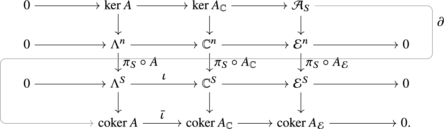
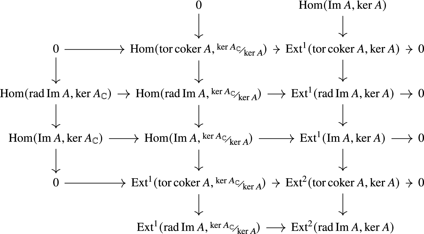
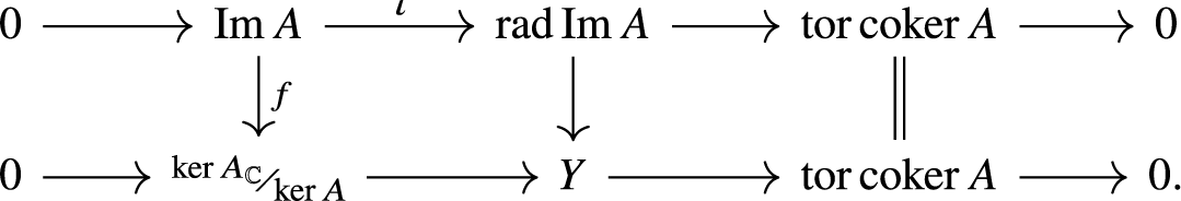
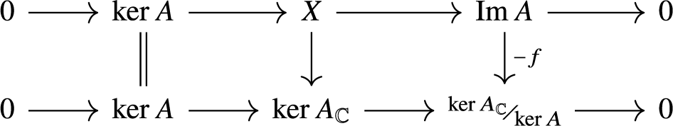
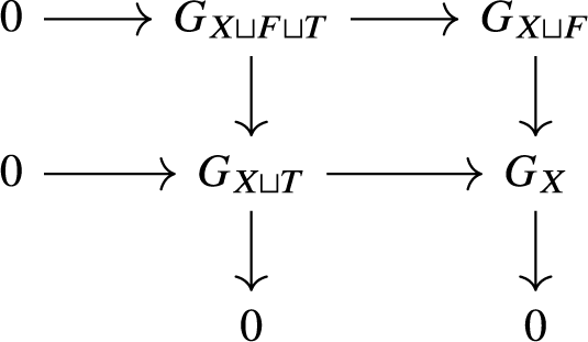
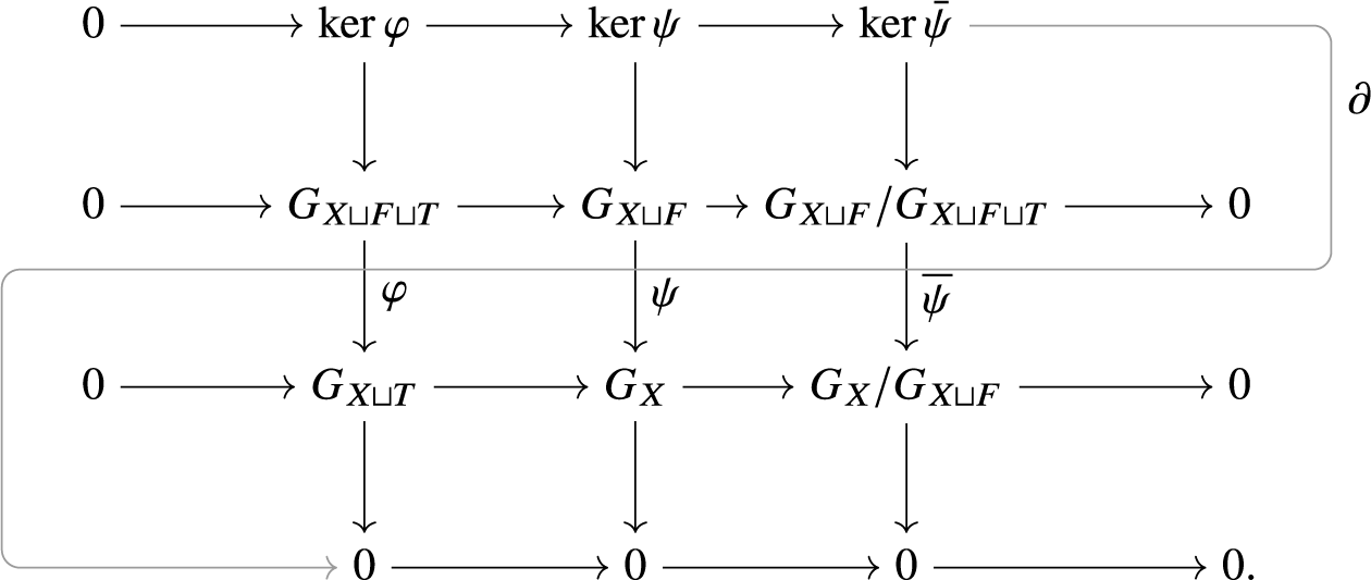

 Open access