





Impact Statement
Offshore wind farms alter the flow of air and water through the extraction of momentum from the atmosphere. This study uses coupled atmosphere–ocean simulations to investigate how momentum extraction by wind farms relates to adjustments in wind wakes and coastal upwelling, a process that brings colder, nutrient-rich water toward the surface and supports marine productivity. The analysis identifies consistent links between the strength of momentum extraction, surface-temperature patterns and subsurface circulation. By framing wind-farm momentum extraction as a control parameter in the coupled air–sea dynamics, the work advances the fundamental understanding of flow physics and provides a basis for interpreting how large-scale wind energy development can influence coastal ocean processes.
1. Introduction
Wind energy, both onshore and offshore, has expanded rapidly worldwide in recent years (Global Wind Energy Council 2025a, b). Along the US Pacific coast, several areas have been leased for offshore project development (Bureau of Ocean Energy Management 2021, 2022). One such area, the Morro Bay lease zone, lies within the California Current System, an eastern boundary upwelling region that supports one of the most biologically productive marine ecosystems globally (Collins et al. Reference Collins, Pennington, Castro, Rago and Chavez2003). Its position at the confluence of persistent alongshore winds, complex coastal topography and strong seasonal upwelling makes the region a representative setting for examining how modifications to the surface wind field influence air–sea coupling. Offshore wind farms provide one example of such modifications, highlighting the broader challenge of understanding how externally imposed changes in wind stress alter the coupled dynamics that sustains coastal upwelling.
Coastal upwelling in eastern boundary current systems arises from alongshore wind stress acting on the ocean surface, which, through the Coriolis effect, drives offshore Ekman transport and the upward advection of cold, nutrient-rich subsurface waters (Capet et al. Reference Capet, Marchesiello and McWilliams2004). In the California Current System, these vertical motions are confined to a narrow coastal band, tens of kilometres wide, and exhibit strong spatio-temporal variability governed by wind forcing, coastline geometry, and stratification (Bakun et al. Reference Bakun, Black, Bograd, Garcia-Reyes, Miller, Rykaczewski and Sydeman2015; Egerer et al. Reference Egerer, Ghate, Miller, Mitra, Xia and Krishnamurthy2026; Wang et al. Reference Wang, Gouhier, Menge and Ganguly2015). Any perturbation to the near-surface wind field, whether from natural variability or anthropogenic structures, has the potential to alter the processes sustaining coastal upwelling.
Offshore wind farms represent such a perturbation. By extracting kinetic energy from the marine atmospheric boundary-layer flow, turbine operation reduces local wind speeds, generates turbine wakes and redistributes surface wind stress. Satellite, in-situ and modelling studies of operating onshore wind farms have documented wake-induced changes in near-surface temperature and turbulent fluxes (Rajewski et al. Reference Rajewski, Takle, Prueger and Doorenbos2016; Zhou et al. Reference Zhou, Tian, Baidya Roy, Thorncroft, Bosart and Hu2012). These effects can extend far beyond the turbine array, modifying surface fluxes, vertical motions and stratification (Broström Reference Broström2008; Carpenter & Guha Reference Carpenter and Guha2024; Floeter et al. Reference Floeter, Pohlmann, Harmer and Möllmann2022; Hasager et al. Reference Hasager, Rasmussen, Peña, Jensen and Réthoré2013; Krishnamurthy et al. Reference Krishnamurthy, Newsom, Kaul, Letizia, Pekour, Hamilton, Chand, Flynn, Bodini and Moriarty2025; Liu et al. Reference Liu, Du, Larsén and Lian2023; Paskyabi Reference Paskyabi2015). Modelling studies further suggest that wind-farm-induced wind-stress anomalies can influence mesoscale circulation, alter the occurrence of marine heatwaves and locally modify cross-shore upwelling patterns in eastern boundary current systems (Dalsin et al. Reference Dalsin, Walter and Mazzini2025; Raghukumar et al. Reference Raghukumar, Nelson, Jacox, Chartrand, Fiechter, Chang, Cheung and Roberts2023). Recent fully coupled ocean–atmosphere–wave simulations by Seo et al. (Reference Seo, Sauvage, Renkl, Lundquist and Kirincich2025) showed that wind-stress reductions over seasonally stratified US East Coast shelves can warm sea-surface temperature (SST) by 0.3–0.4 $^\circ$
C and shoal the mixed layer. In those simulations, the SST warming increased upward heat fluxes and fed back on the atmospheric boundary layer, illustrating the need to retain two-way air–sea coupling when interpreting wind-farm effects on the upper ocean. A unifying description of these impacts is that offshore wind farms act as distributed drag elements in the atmospheric boundary layer, extracting momentum and modifying surface stress patterns. Formulating wind-farm effects in terms of a distributed drag force on the atmospheric boundary layer offers a fluid-mechanical basis for connecting turbine-scale momentum extraction to mesoscale atmospheric and oceanic responses.
$^\circ$
C and shoal the mixed layer. In those simulations, the SST warming increased upward heat fluxes and fed back on the atmospheric boundary layer, illustrating the need to retain two-way air–sea coupling when interpreting wind-farm effects on the upper ocean. A unifying description of these impacts is that offshore wind farms act as distributed drag elements in the atmospheric boundary layer, extracting momentum and modifying surface stress patterns. Formulating wind-farm effects in terms of a distributed drag force on the atmospheric boundary layer offers a fluid-mechanical basis for connecting turbine-scale momentum extraction to mesoscale atmospheric and oceanic responses.
The sensitivity of wind-driven upwelling to offshore wind turbine-induced drag, however, remains poorly understood. Previous studies have examined specific wind-farm layouts or turbine designs (e.g. Gaumond & Réthoré Reference Gaumond and Réthoré2014; Quint et al. Reference Quint, Lundquist, Bodini and Rosencrans2025; Raghukumar et al. Reference Raghukumar, Nelson, Jacox, Chartrand, Fiechter, Chang, Cheung and Roberts2023). However, to the best of our knowledge, no systematic assessment has quantified how the upwelling response varies across a physically plausible range of drag magnitudes in a realistic coastal setting. A mechanistic understanding of this sensitivity is essential for predicting the local and broader oceanic consequences of wind energy development.
Here, we address this gap by representing turbines through an idealised, height-varying drag parameterisation embedded in a high-resolution coupled atmosphere–ocean model. This approach isolates the leading-order fluid-dynamical impact of momentum extraction while avoiding dependence on specific turbine designs. Using the coupled ocean–atmosphere–wave–sediment transport (COAWST) modelling system developed by Warner et al. (Reference Warner, Armstrong, He and Zambon2010), we perform month-long simulations of the central California coast across a range of drag scenarios in the Morro Bay lease area. We analyse wind-speed reduction, ocean mixed-layer depth, ocean vertical velocity and SST anomalies to quantify how turbine drag modifies the strength and spatial structure of coastal upwelling.
The central question of this study is how externally imposed momentum extraction in the atmospheric boundary layer alters the fluid-dynamical pathways that drive coastal upwelling in the ocean. Offshore wind farms provide a suitable setting in which such perturbations occur, and we use this configuration to investigate a canonical problem in a real-world setting: the response of the coastal upwelling system to systematically varied surface drag. By varying the drag parameter, we quantify both the atmospheric adjustment and the coupled oceanic consequences, thereby identifying the potential threshold behaviour and scaling laws that govern drag-induced upwelling perturbations.
The remainder of the paper is organised as follows. Section 2 describes the problem set-up, including model configuration and experimental design. Section 3 presents the results, focusing on the influence of wind-farm-induced momentum extraction on air–sea characteristics. Conclusions are given in Section 4.
2. Problem set-up
2.1. Numerical methods and model configuration
The study employs a high-resolution coupled mesoscale modelling framework to resolve the coupled interactions between atmosphere, ocean and surface waves. Three established geophysical-flow models are integrated within the COAWST system (Warner et al. Reference Warner, Armstrong, He and Zambon2010), each resolving distinct components of the coupled air–sea interactions. We give schematic momentum/action balances to define the principal terms used in the analysis; the complete numerical formulations, parameterisations and boundary conditions are given in the Supplementary Material.
2.1.1. Atmospheric model (WRF)
The atmospheric flow is simulated using the weather research and forecasting (WRF) model (Skamarock et al. Reference Skamarock, Klemp, Dudhia, Gill, Liu, Berner, Wang, Powers, Duda, Barker and Huang2019), which solves the compressible, non-hydrostatic Euler equations on a terrain-following hydrostatic-pressure vertical coordinate. Schematically, the horizontal momentum balance takes the flux form
 \begin{align} \frac {\partial (\rho ^a u_i^a)}{\partial t} + \frac {\partial (\rho ^a u_i^a u_j^a)}{\partial x_j} = -\frac {\partial p^a}{\partial x_i} + \rho ^a f\epsilon _{\textit{ij}3}u_j^a + \frac {\partial }{\partial z}\!\left (\rho ^a\nu _t\frac {\partial u_i^a}{\partial z}\right ) + \rho ^a F_i, \quad i=1,2, \end{align}
where $u_i^a$
is the horizontal air velocity,
$u_i^a$
is the horizontal air velocity, $\rho ^a$
is air density,
$\rho ^a$
is air density, $p^a$
is atmospheric pressure,
$p^a$
is atmospheric pressure, $f$
is the Coriolis parameter,
$f$
is the Coriolis parameter, $\nu _t$
is the turbulent eddy viscosity provided by the planetary boundary-layer scheme and
$\nu _t$
is the turbulent eddy viscosity provided by the planetary boundary-layer scheme and $F_i$
is an external body force used in Section 2.2 to represent wind-farm drag. The full terrain-following flux-form equations that the WRF model actually integrates, including the mass-coupled prognostic variables and the diagnostic equation of state, are given in Section S2 of the Supplementary Material. Planetary boundary-layer turbulence is parameterised using the Yonsei University scheme (Hong et al. Reference Hong, Noh and Dudhia2006). The WRF model is initialised and forced at its lateral boundaries using fifth-generation European Centre for Medium-Range Weather Forecasts atmospheric reanalysis (ERA5) reanalysis data (Hersbach et al. Reference Hersbach, Bell, Berrisford, Hirahara, Horányi, Muñoz‐Sabater, Nicolas, Peubey, Radu, Schepers, Simmons, Soci, Abdalla, Abellan, Balsamo, Bechtold, Biavati, Bidlot, Bonavita, De Chiara, Dahlgren, Dee, Diamantakis, Dragani, Flemming, Forbes, Fuentes, Geer, Haimberger, Healy, Hogan, Hólm, Janisková, Keeley, Laloyaux, Lopez, Lupu, Radnoti, de Rosnay, Rozum, Vamborg, Villaume and Thépaut2020), with grid nudging applied above the boundary layer to maintain large-scale synoptic conditions. The full initial and boundary-condition set-up, including the nudging formulation and rates, is detailed in Section S4 of the Supplementary Material. Terrain elevation data are obtained from the United States Geological Survey (USGS) high-resolution topography dataset during WRF model preprocessing.
$F_i$
is an external body force used in Section 2.2 to represent wind-farm drag. The full terrain-following flux-form equations that the WRF model actually integrates, including the mass-coupled prognostic variables and the diagnostic equation of state, are given in Section S2 of the Supplementary Material. Planetary boundary-layer turbulence is parameterised using the Yonsei University scheme (Hong et al. Reference Hong, Noh and Dudhia2006). The WRF model is initialised and forced at its lateral boundaries using fifth-generation European Centre for Medium-Range Weather Forecasts atmospheric reanalysis (ERA5) reanalysis data (Hersbach et al. Reference Hersbach, Bell, Berrisford, Hirahara, Horányi, Muñoz‐Sabater, Nicolas, Peubey, Radu, Schepers, Simmons, Soci, Abdalla, Abellan, Balsamo, Bechtold, Biavati, Bidlot, Bonavita, De Chiara, Dahlgren, Dee, Diamantakis, Dragani, Flemming, Forbes, Fuentes, Geer, Haimberger, Healy, Hogan, Hólm, Janisková, Keeley, Laloyaux, Lopez, Lupu, Radnoti, de Rosnay, Rozum, Vamborg, Villaume and Thépaut2020), with grid nudging applied above the boundary layer to maintain large-scale synoptic conditions. The full initial and boundary-condition set-up, including the nudging formulation and rates, is detailed in Section S4 of the Supplementary Material. Terrain elevation data are obtained from the United States Geological Survey (USGS) high-resolution topography dataset during WRF model preprocessing.
2.1.2. Ocean model (ROMS)
Ocean circulation is modelled through the regional ocean modelling system (ROMS), which solves the hydrostatic primitive equations under the Boussinesq approximation (Shchepetkin & McWilliams Reference Shchepetkin and McWilliams2005). The horizontal momentum equations take the form
 \begin{align} \frac {\partial u^o}{\partial t} + \boldsymbol{u}^o\cdot \nabla u^o - fv^o &= -\frac {1}{\rho _0}\frac {\partial p^o}{\partial x} + \frac {\partial }{\partial z}\!\left (K_m\frac {\partial u^o}{\partial z}\right ) + \mathcal{D}_u, \\[-12pt] \nonumber \end{align}
 \begin{align} \frac {\partial v^o}{\partial t} + \boldsymbol{u}^o\cdot \nabla v^o + fu^o &= -\frac {1}{\rho _0}\frac {\partial p^o}{\partial y} + \frac {\partial }{\partial z}\!\left (K_m\frac {\partial v^o}{\partial z}\right ) + \mathcal{D}_v, \\[10pt] \nonumber \end{align}
where $(u^o, v^o)$
are the horizontal components of the ocean velocity
$(u^o, v^o)$
are the horizontal components of the ocean velocity $\boldsymbol{u}^o$
,
$\boldsymbol{u}^o$
, $p^o$
is the ocean pressure,
$p^o$
is the ocean pressure, $\rho _0$
is a constant reference density,
$\rho _0$
is a constant reference density, $K_m$
is the vertical eddy viscosity and
$K_m$
is the vertical eddy viscosity and $\mathcal{D}_u, \mathcal{D}_v$
represent horizontal diffusion and other sub-grid-scale terms acting on the ocean momentum. These are supplemented by the hydrostatic relation
$\mathcal{D}_u, \mathcal{D}_v$
represent horizontal diffusion and other sub-grid-scale terms acting on the ocean momentum. These are supplemented by the hydrostatic relation $\partial p^o/\partial z = -\rho ^o g$
, where $g$ is the gravitational acceleration, the incompressibility condition
$\partial p^o/\partial z = -\rho ^o g$
, where $g$ is the gravitational acceleration, the incompressibility condition $\nabla \cdot \boldsymbol{u}^o=0$
and tracer conservation equations for temperature and salinity (see Supplementary Material). The model employs a stretched terrain-following (sigma) coordinate system with 40 vertical levels, providing enhanced resolution near the surface and bottom boundary layers. Vertical mixing is parameterised by the generic length scale two-equation turbulence closure (Umlauf & Burchard Reference Umlauf and Burchard2003) with Kantha–Clayson stability functions (Kantha & Clayson Reference Kantha and Clayson1994). The ROMS is initialised from an antecedent multi-year simulation (Hinson et al. Reference Hinson, Gaudet, Li, Hetland, Mirocha, Yang and Krishnamurthy2026), which provides temperature, salinity, velocity and sea-surface height for both the initial condition and the open lateral boundaries. The specific boundary-condition schemes applied to each prognostic field are detailed in Section S4 of the Supplementary Material.
$\nabla \cdot \boldsymbol{u}^o=0$
and tracer conservation equations for temperature and salinity (see Supplementary Material). The model employs a stretched terrain-following (sigma) coordinate system with 40 vertical levels, providing enhanced resolution near the surface and bottom boundary layers. Vertical mixing is parameterised by the generic length scale two-equation turbulence closure (Umlauf & Burchard Reference Umlauf and Burchard2003) with Kantha–Clayson stability functions (Kantha & Clayson Reference Kantha and Clayson1994). The ROMS is initialised from an antecedent multi-year simulation (Hinson et al. Reference Hinson, Gaudet, Li, Hetland, Mirocha, Yang and Krishnamurthy2026), which provides temperature, salinity, velocity and sea-surface height for both the initial condition and the open lateral boundaries. The specific boundary-condition schemes applied to each prognostic field are detailed in Section S4 of the Supplementary Material.
2.1.3. Wave model (WW3)
Surface wave dynamics is resolved by WaveWatch III (WW3) (Tolman Reference Tolman2009), which integrates the spectral wave action balance equation
 \begin{align} \frac {\partial N}{\partial t} + \nabla _{\boldsymbol{x}}\cdot (\dot {\boldsymbol{x}}N) + \frac {\partial }{\partial k}(\dot {k}N) + \frac {\partial }{\partial \theta }(\dot {\theta }N) = \frac {S_{tot}}{\sigma }, \end{align}
where $N(k,\theta ;\boldsymbol{x},t)=E(k,\theta ;\boldsymbol{x},t)/\sigma$
is the wave action spectral density,
$N(k,\theta ;\boldsymbol{x},t)=E(k,\theta ;\boldsymbol{x},t)/\sigma$
is the wave action spectral density, $E$
is the wave energy spectral density,
$E$
is the wave energy spectral density, $k$
is the wavenumber magnitude,
$k$
is the wavenumber magnitude, $\theta$
is wave direction and
$\theta$
is wave direction and $\sigma$
is the intrinsic angular frequency. The physical-space propagation velocity is
$\sigma$
is the intrinsic angular frequency. The physical-space propagation velocity is $\dot {\boldsymbol{x}}=\boldsymbol{c}_g+\boldsymbol{U}$
, where
$\dot {\boldsymbol{x}}=\boldsymbol{c}_g+\boldsymbol{U}$
, where $\boldsymbol{c}_g=\partial \sigma /\partial \boldsymbol{k}$
is the intrinsic group velocity and
$\boldsymbol{c}_g=\partial \sigma /\partial \boldsymbol{k}$
is the intrinsic group velocity and $\boldsymbol{U}$
is the ambient current supplied by ROMS. The spectral propagation terms
$\boldsymbol{U}$
is the ambient current supplied by ROMS. The spectral propagation terms $\dot {k}$
and
$\dot {k}$
and $\dot {\theta }$
represent shoaling and refraction by depth and current gradients, and
$\dot {\theta }$
represent shoaling and refraction by depth and current gradients, and $S_{tot}$
collects source terms for wind input, nonlinear wave–wave interactions and dissipation. WaveWatch III is initialised with a calm sea surface and evolves under wind forcing provided by the WRF model and surface currents from ROMS. The spectral discretisation and lateral-boundary treatment are detailed in Section S4 of the Supplementary Material. WaveWatch III is included in the coupled system to provide a sea-state-dependent surface roughness
$S_{tot}$
collects source terms for wind input, nonlinear wave–wave interactions and dissipation. WaveWatch III is initialised with a calm sea surface and evolves under wind forcing provided by the WRF model and surface currents from ROMS. The spectral discretisation and lateral-boundary treatment are detailed in Section S4 of the Supplementary Material. WaveWatch III is included in the coupled system to provide a sea-state-dependent surface roughness $z_0$
to the WRF model surface layer via the Taylor–Yelland parameterisation, which uses significant wave height and wavelength rather than a fixed Charnock relation. In the remainder of the paper, the superscripts
$z_0$
to the WRF model surface layer via the Taylor–Yelland parameterisation, which uses significant wave height and wavelength rather than a fixed Charnock relation. In the remainder of the paper, the superscripts $a$
and
$a$
and $o$
are omitted for readability.
$o$
are omitted for readability.
Model domain and terrain elevation along the US West Coast. Terrain height over land and 10 m wind speed over the ocean are shown from the baseline COAWST simulation (no turbine drag). Separate colour scales are used for land and ocean fields. The orange rectangle indicates the wind-farm drag region, approximating the Morro Bay Wind Energy Lease Area (the actual lease boundaries are irregular). The illustration is based on the instantaneous field from the results at 04:00 UTC on 17 May 2021.

Figure 1 Long description
A heat map showing terrain height over land and wind speed over the ocean along the US West Coast. The map uses separate color scales for land and ocean fields. The terrain height over land ranges from 0 to 3600 meters, with higher elevations shown in darker colors and lower elevations in lighter colors. The wind speed over the ocean ranges from 0 to 14 meters per second, with higher wind speeds shown in darker colors and lower wind speeds in lighter colors. An orange rectangle indicates the wind-farm drag region, approximating the Morro Bay Wind Energy Lease Area. The map is based on the instantaneous field from the results at 04:00 UTC on 17 May 2021.
2.1.4. Model grid, coupling and baseline wind climatology
All three models within the COAWST framework operate on uniform 1-km horizontal grids spanning the California coastal region, with particular focus on the Morro Bay Wind Energy Lease Area. The computational grid points are $700\times 800\times 90$
for the WRF model,
$700\times 800\times 90$
for the WRF model, $696\times 796\times 40$
for ROMS and
$696\times 796\times 40$
for ROMS and $696\times 796$
for WW3, where the first two indices represent horizontal extent in longitude and latitude, respectively, and the third indices for the WRF model and ROMS represent the vertical grid points. Figure 1 illustrates the computational domain and representative atmospheric fields, with terrain elevation visible along the coastal mountain ranges and the baseline wind field over the ocean exhibiting the persistent northwesterly regime. The seabed bathymetry of the ROMS domain is shown in figure S1 of the Supplementary Material.
$696\times 796$
for WW3, where the first two indices represent horizontal extent in longitude and latitude, respectively, and the third indices for the WRF model and ROMS represent the vertical grid points. Figure 1 illustrates the computational domain and representative atmospheric fields, with terrain elevation visible along the coastal mountain ranges and the baseline wind field over the ocean exhibiting the persistent northwesterly regime. The seabed bathymetry of the ROMS domain is shown in figure S1 of the Supplementary Material.
Model components are coupled through the model coupling toolkit with a state-variable exchange every 600 s (Warner et al. Reference Warner, Perlin and Skyllingstad2008). The WRF model computes the surface momentum stress and turbulent heat fluxes internally within its surface-layer scheme, with wave-dependent surface roughness supplied by WW3 via the Taylor–Yelland parameterisation. The WRF model then passes to ROMS the surface stress components, the sensible and latent heat fluxes, the net shortwave and downward longwave radiation, sea-level pressure, precipitation and evaporation. The ROMS receives these as flux fields at its surface boundary and does not invoke its own bulk-flux scheme. The ROMS returns SST to the WRF model as the lower boundary condition for the atmospheric surface-layer calculation. The WRF model also passes 10-m wind fields to WW3, which returns significant wave height and wavelength to the WRF model for use in the Taylor–Yelland wave-dependent roughness formulation. The ROMS provides surface currents and sea-surface elevation to WW3, which returns wave height, wavelength, wave direction, wave periods and wave energy dissipation channels to ROMS for use in its vortex-force wave-effects-on-currents module (Kumar et al. Reference Kumar, Voulgaris, Warner and Olabarrieta2012; Uchiyama et al. Reference Uchiyama, McWilliams and Shchepetkin2010). This two-way coupling among all three components ensures that atmosphere–ocean–wave feedbacks are represented at each exchange interval. The full list of exchanged variables and their physical roles is given in Table S2 of the Supplementary Material. The assessment of the present numerical framework with field observations is detailed in Gaudet et al. (Reference Gaudet, Liu, Hinson, Hetland, Krishnamurthy, Yang, Li, Mirocha, Xia, Hendricks and Juliano2026).
The baseline wind climatology over the Morro Bay lease area for the 1–31 May 2021 study period is summarised in figure 2. Hub-height winds at $\sim$
150 m are persistent and dominated by the northwesterly sector: 97 % of samples originate from directions between due west and due north. The stick plot shows that this northwesterly (NW) regime is near continuous throughout the month, with only a brief relaxation event in mid-May. This persistent NW wind regime provides the background state against which all wind-farm perturbation cases in Section 3 are evaluated. The corresponding marine atmospheric boundary layer is predominantly near neutral to weakly unstable, with brief stable excursions associated with synoptic wind relaxations. Details of the air–sea temperature difference diagnostic are provided in Section S6 of the Supplementary Material.
$\sim$
150 m are persistent and dominated by the northwesterly sector: 97 % of samples originate from directions between due west and due north. The stick plot shows that this northwesterly (NW) regime is near continuous throughout the month, with only a brief relaxation event in mid-May. This persistent NW wind regime provides the background state against which all wind-farm perturbation cases in Section 3 are evaluated. The corresponding marine atmospheric boundary layer is predominantly near neutral to weakly unstable, with brief stable excursions associated with synoptic wind relaxations. Details of the air–sea temperature difference diagnostic are provided in Section S6 of the Supplementary Material.
Baseline wind climatology over the Morro Bay lease area, 1–31 May 2021. (a) Wind rose of hub-height winds, pooled across all lease grid points and 2-hourly time steps. (b) Stick plot of lease-mean hub-height wind vectors over the same period. Stick angle matches the true wind direction, stick length is proportional to wind speed, and colour indicates the hub-height wind speed $|\vec {U}_{\mathrm{hub}}|$
.
$|\vec {U}_{\mathrm{hub}}|$
.

2.2. Turbine drag parameterisation
Several detailed mesoscale wind-farm parameterisations have been developed in over the last decade, most notably the Fitch scheme (Fitch et al. Reference Fitch, Olson, Lundquist, Dudhia, Gupta, Michalakes and Barstad2012), which resolves wake recovery processes and turbine-scale turbulence effects. The wake-added turbulence in particular has been shown to influence near-surface temperature in the onshore context (Tomaszewski & Lundquist Reference Tomaszewski and Lundquist2020). Such models are well suited for quantifying power production or wake behaviour. In the present context, however, the complexity of the fully coupled atmosphere–ocean system already poses significant challenges for interpretation. Introducing additional turbine-scale parameterisation would add further sensitivities that could complicate the attribution of the response to momentum extraction as its leading-order driver.
For clarity, we refer to our deliberately idealised parameterisation as the generalised turbine drag (GTD) model. It prescribes a simple, height-dependent drag profile that represents the aggregate momentum sink of a wind-farm canopy. This formulation captures the dominant dynamical influence, namely the reduction of atmospheric momentum, while avoiding case-specific assumptions about turbine design, layout or control strategies. In this way, the offshore wind farm is treated not as an engineering system, but as a canonical forcing mechanism acting on the marine atmospheric boundary layer.
Within this framework, wind turbine effects are represented by prescribing a height-varying drag coefficient in the momentum equations of the WRF model over the designated wind-farm region. For simplicity, the wind-farm region is taken as the smallest rectangular domain fully enclosing the Morro Bay lease area, recognising that the actual lease boundaries are more complex. The imposed drag acts as a vertically distributed momentum sink that emulates the first-order effect of a large offshore wind farm. By varying the drag magnitude across a suite of simulations, we systematically assess the sensitivity of the coupled atmosphere–ocean system to externally imposed momentum extraction.
Mathematically, the drag is imposed through an additional body force in the WRF model momentum equations
 \begin{align} F_i = -C_d(z) u_i |\boldsymbol{u}|, \qquad i=1,2,3, \end{align}
where $\boldsymbol{u}=(u,v,w)$
is the local resolved air velocity,
$\boldsymbol{u}=(u,v,w)$
is the local resolved air velocity, $|\boldsymbol{u}|=(u^2+v^2+w^2)^{1/2}$
is the corresponding wind-speed magnitude and
$|\boldsymbol{u}|=(u^2+v^2+w^2)^{1/2}$
is the corresponding wind-speed magnitude and $C_d(z)$
is the prescribed height-dependent drag-density coefficient, with units of
$C_d(z)$
is the prescribed height-dependent drag-density coefficient, with units of $\mathrm{m}^{-1}$
; for brevity, we refer to
$\mathrm{m}^{-1}$
; for brevity, we refer to $C_d$
hereafter as the drag coefficient. The quadratic form makes the imposed force oppose the local resolved velocity vector and scale with the local kinetic momentum flux, consistent with an idealised canopy- or porous-drag representation of turbine-induced momentum extraction. The body force
$C_d$
hereafter as the drag coefficient. The quadratic form makes the imposed force oppose the local resolved velocity vector and scale with the local kinetic momentum flux, consistent with an idealised canopy- or porous-drag representation of turbine-induced momentum extraction. The body force $F_i$
is added directly to the WRF model momentum tendencies for all three velocity components at vertical levels in the lease-area grid columns where
$F_i$
is added directly to the WRF model momentum tendencies for all three velocity components at vertical levels in the lease-area grid columns where $C_d(z)$
is non-negligible (approximately 0–300 m), and at no other grid points. Unlike the Fitch parameterisation, the GTD does not inject additional turbulent kinetic energy into the planetary boundary layer (PBL) scheme; the resulting boundary-layer turbulence therefore arises from the atmospheric adjustment to the prescribed momentum sink alone. The value of
$C_d(z)$
is non-negligible (approximately 0–300 m), and at no other grid points. Unlike the Fitch parameterisation, the GTD does not inject additional turbulent kinetic energy into the planetary boundary layer (PBL) scheme; the resulting boundary-layer turbulence therefore arises from the atmospheric adjustment to the prescribed momentum sink alone. The value of $C_d$
sets the overall strength of momentum extraction by the wind farm, and is independent of turbine spacing, rotor diameter or thrust curve. The GTD therefore prescribes a spatially distributed, vertically varying momentum sink over the lease area, analogous to a canopy-drag formulation in plant or urban boundary-layer studies, isolating the role of total momentum extraction as a control parameter in the coupled system, independent of a particular turbine layout.
$C_d$
sets the overall strength of momentum extraction by the wind farm, and is independent of turbine spacing, rotor diameter or thrust curve. The GTD therefore prescribes a spatially distributed, vertically varying momentum sink over the lease area, analogous to a canopy-drag formulation in plant or urban boundary-layer studies, isolating the role of total momentum extraction as a control parameter in the coupled system, independent of a particular turbine layout.
The drag coefficient $C_d(z)$
is specified as a Gaussian-like function of height, centred at
$C_d(z)$
is specified as a Gaussian-like function of height, centred at $z_h = 150$
m, which represents the typical hub height of next-generation
$z_h = 150$
m, which represents the typical hub height of next-generation $\sim$
15 MW offshore turbines, such as the IEA 15 MW reference turbine with a rotor diameter of approximately 240 m. The distribution decays smoothly above and below
$\sim$
15 MW offshore turbines, such as the IEA 15 MW reference turbine with a rotor diameter of approximately 240 m. The distribution decays smoothly above and below $z_h$
, with appreciable values across roughly 0–300 m, reflecting the fact that momentum extraction is strongest within the rotor-swept layer and diminishes toward the ground and the upper boundary layer. This profile ensures that the drag acts primarily across the vertical extent of the turbine array while avoiding discontinuities that would complicate the coupled dynamics. For simplicity, we later denote
$z_h$
, with appreciable values across roughly 0–300 m, reflecting the fact that momentum extraction is strongest within the rotor-swept layer and diminishes toward the ground and the upper boundary layer. This profile ensures that the drag acts primarily across the vertical extent of the turbine array while avoiding discontinuities that would complicate the coupled dynamics. For simplicity, we later denote $C_d\equiv C_d(z_h)=\max _z C_d(z)$
the hub-height (peak) drag coefficient. The vertical shape is fixed across cases and only the amplitude
$C_d\equiv C_d(z_h)=\max _z C_d(z)$
the hub-height (peak) drag coefficient. The vertical shape is fixed across cases and only the amplitude $C_d$
is varied. The Gaussian-like vertical profile is chosen to concentrate momentum extraction within the rotor-swept layer without requiring assumptions about internal wake equilibrium, unlike the equilibrium-derived mean velocity profile of Stevens & Meneveau (Reference Stevens and Meneveau2017), which is developed for a horizontally homogeneous, fully developed wind-farm boundary layer. The sensitivity analysis here therefore targets the magnitude of the vertically integrated momentum sink rather than its vertical distribution. As a single-parameter model, the GTD holds
$C_d$
is varied. The Gaussian-like vertical profile is chosen to concentrate momentum extraction within the rotor-swept layer without requiring assumptions about internal wake equilibrium, unlike the equilibrium-derived mean velocity profile of Stevens & Meneveau (Reference Stevens and Meneveau2017), which is developed for a horizontally homogeneous, fully developed wind-farm boundary layer. The sensitivity analysis here therefore targets the magnitude of the vertically integrated momentum sink rather than its vertical distribution. As a single-parameter model, the GTD holds $C_d$
constant for all wind speeds and therefore does not represent wind-speed-dependent thrust,
$C_d$
constant for all wind speeds and therefore does not represent wind-speed-dependent thrust, $C_T(U)$
, turbine cut-in or cut-out or other wind-speed-dependent operational behaviours of real turbines. We prescribe ten GTD cases with
$C_T(U)$
, turbine cut-in or cut-out or other wind-speed-dependent operational behaviours of real turbines. We prescribe ten GTD cases with $C_d$
values logarithmically spaced from
$C_d$
values logarithmically spaced from $8.6\times 10^{-7}\,$
(GTD-1) to
$8.6\times 10^{-7}\,$
(GTD-1) to $3.0\times 10^{-5}\,\mathrm{m}^{-1}$
(GTD-10), i.e. a geometric sequence with common ratio of
$3.0\times 10^{-5}\,\mathrm{m}^{-1}$
(GTD-10), i.e. a geometric sequence with common ratio of $1.48$
. The case index therefore increases monotonically with drag strength. The lower bound is chosen so that the resulting hub-height wind-speed deficit is comparable to the model’s noise level, providing a near-zero forcing case at the bottom of the sweep. The upper bound produces hub-height deficits of approximately 15 %–20 %, representing strong momentum extraction at the upper end expected from dense offshore wind-farm deployments. The resulting sweep is sampled uniformly on a logarithmic axis and spans the linear-scaling regime and any threshold transitions in the coupled response.
$1.48$
. The case index therefore increases monotonically with drag strength. The lower bound is chosen so that the resulting hub-height wind-speed deficit is comparable to the model’s noise level, providing a near-zero forcing case at the bottom of the sweep. The upper bound produces hub-height deficits of approximately 15 %–20 %, representing strong momentum extraction at the upper end expected from dense offshore wind-farm deployments. The resulting sweep is sampled uniformly on a logarithmic axis and spans the linear-scaling regime and any threshold transitions in the coupled response.
This idealised parameterisation offers two key advantages. First, it isolates the fundamental role of turbine drag as a control parameter within the coastal dynamical system, enabling systematic exploration across a wide range of drag strengths. Second, it provides a framework for deriving scaling laws and thresholds governing wind-farm-induced modifications to coastal upwelling, without conflating those responses with turbine-specific engineering details.
The GTD is introduced in this study as a deliberately idealised, single-parameter representation of turbine momentum extraction, rather than an attempt to reproduce a specific operational wind farm. The formulation isolates the first-order effect of turbine-induced momentum extraction and treats turbine-specific parameters such as thrust curves and wake-added turbulent kinetic energy (TKE) as outside the leading-order control parameter explored here. This hierarchy is consistent with the recent finding of Seo et al. (Reference Seo, Sauvage, Renkl, Lundquist and Kirincich2025) that the wake-induced SST response shows weak dependence on the wake-added TKE parameter in offshore coupled simulations. The ten-case sweep from GTD-1 to GTD-10 itself spans 1.5 orders of magnitude in drag strength and constitutes a systematic sensitivity analysis with respect to the amplitude of the momentum sink. A systematic hierarchical comparison with more detailed parameterisations is beyond the scope of the present study.
We note that the Morro Bay lease area lies in water depths of approximately 1000 m on average (Johnson et al. Reference Johnson, Currier, Howar, Elliott, Rockwood and Jahncke2022), where only floating platforms are feasible. Unlike fixed-bottom turbines, floating turbines are not anchored to the seabed by rigid foundations, so any direct mechanical forcing on the surrounding ocean is expected to be small (Farr et al. Reference Farr, Ruttenberg, Walter, Wang and White2021). The present simulations therefore do not include such direct mechanical forcing.
2.3. Data processing and analysis
All simulations are conducted over a one-month period spanning from 27 April to 31 May 2021, a season characterised by persistent upwelling-favourable winds along the central California coast and in the Morro Bay area (Egerer et al. Reference Egerer, Ghate, Miller, Mitra, Xia and Krishnamurthy2026). This interval was selected because it also includes a variety of representative weather regimes. The first four days are discarded as model spin-up, leaving a 30-day window in which the coupled system exhibits sustained, dynamically relevant variability. In total, ten GTD cases and one baseline simulation were conducted, with GTD-1 corresponding to the lowest drag and GTD-10 to the highest. All simulations were performed on the U.S. Department of Energy (DOE) supercomputer at the United States National Laboratory of the Rockies, with a total computational cost of approximately $3.41 \times 10^{6}$
CPU hours. Atmospheric fields from the WRF model were output every 2 h and ocean fields from ROMS every 1.5 h, providing sufficient temporal resolution for the month-long analyses.
$3.41 \times 10^{6}$
CPU hours. Atmospheric fields from the WRF model were output every 2 h and ocean fields from ROMS every 1.5 h, providing sufficient temporal resolution for the month-long analyses.
Time averaging is used to isolate the quasi-steady mesoscale response of the coupled system to turbine-induced drag. For most diagnostics we compute 30-day means, which filter high-frequency weather fluctuations and reveal systematic modifications to atmosphere–ocean exchange. To examine the temporal development of these responses, we also partition the analysis into three non-overlapping intervals (days 1–10, 11–20 and 21–30 after spin-up). This separation allows us to distinguish persistent dynamical features from transient fluctuations and to assess whether wind-farm impacts intensify or saturate with time.
Diagnostics are chosen to characterise both the atmospheric and oceanic pathways by which turbine drag modifies upwelling. Horizontal wind-speed fields quantify momentum extraction and its downstream extent, while surface sensible and latent heat fluxes describe changes to air–sea exchange. On the ocean side, we compute SST anomalies, mixed-layer depth (MLD) and vertical velocity at MLD base as indicators of stratification and upwelling strength. To isolate wind-farm-induced anomalies, each case is compared with a common baseline simulation with no additional turbine drag.
Finally, the spatial patterns of SST response are extracted using an empirical orthogonal function (EOF) decomposition. This approach identifies the leading-order dipole-like mode associated with wind-farm forcing and provides a compact metric of its amplitude across drag cases. By projecting each SST anomaly field onto this dominant mode, we obtain a scalar coefficient that quantifies how strongly the canonical dipole pattern is expressed in that case; this coefficient serves as a compact metric of the wind-farm-forced SST response across different drag cases. The EOF projection thus serves as a systematic measure of the canonical SST response, complementing direct inspection of anomaly fields.
These diagnostics provide a consistent framework for comparing cases across the full range of turbine drag strengths, setting the stage for the results that follow on wind-speed scaling, influence-zone expansion and the emergence of dipole-like SST anomalies.
3. Results and discussions
The response of the coupled atmosphere–ocean system is examined as a function of turbine drag strength. We first assess the reduction of wind speed and its scaling with drag. We then quantify the spatial extent of the wind-farm influence zone before turning to oceanic adjustments, including SST anomalies, vertical velocity and MLD. To separate persistent signals from transient variability, results are presented using both 30-day means and averages over successive 10-day windows.
( $a$
) Temporal evolution of hub-height mean wind speed over the wind-farm area for all GTD scenarios compared with the baseline case, obtained from the COAWST simulations. (
$a$
) Temporal evolution of hub-height mean wind speed over the wind-farm area for all GTD scenarios compared with the baseline case, obtained from the COAWST simulations. ( $b$
) Vertical profile of the drag coefficient
$b$
) Vertical profile of the drag coefficient $C_d(z)$
prescribed in each GTD case. Drag increases monotonically from GTD-1 (hub height
$C_d(z)$
prescribed in each GTD case. Drag increases monotonically from GTD-1 (hub height $C_d = 8.6\times 10^{-7}\,\mathrm{m}^{-1}$
) to GTD-10 (
$C_d = 8.6\times 10^{-7}\,\mathrm{m}^{-1}$
) to GTD-10 ( $C_d = 3.0\times 10^{-5}\,\mathrm{m}^{-1}$
), with values logarithmically spaced. The dashed line marks the hub height (150 m).
$C_d = 3.0\times 10^{-5}\,\mathrm{m}^{-1}$
), with values logarithmically spaced. The dashed line marks the hub height (150 m).

3.1. Wind-speed modification by turbine-induced drag
The generalised turbine drag produces a systematic reduction in wind speed across all simulations. Figure 3 shows ( $a$
) the temporal evolution of hub-height mean wind speed over the wind-farm area for all GTD cases compared with the baseline, and (
$a$
) the temporal evolution of hub-height mean wind speed over the wind-farm area for all GTD cases compared with the baseline, and ( $b$
) the prescribed vertical profile of the drag coefficient
$b$
) the prescribed vertical profile of the drag coefficient $C_d(z)$
in each case. Synoptic variability produces large temporal fluctuations in wind speed, but across all GTD cases a systematic separation is maintained: stronger drag consistently leads to greater mean wind-speed reductions. This indicates that turbine-induced momentum extraction imposes a persistent perturbation superimposed on the background atmospheric variability.
$C_d(z)$
in each case. Synoptic variability produces large temporal fluctuations in wind speed, but across all GTD cases a systematic separation is maintained: stronger drag consistently leads to greater mean wind-speed reductions. This indicates that turbine-induced momentum extraction imposes a persistent perturbation superimposed on the background atmospheric variability.
The magnitude of the wind-speed deficit increases monotonically with drag strength. Figure 4 shows the normalised hub-height wind-speed reduction, $(1-U/U_0)$
, plotted against the drag coefficient at hub height,
$(1-U/U_0)$
, plotted against the drag coefficient at hub height, $C_d$
, on logarithmic axes. Here,
$C_d$
, on logarithmic axes. Here, $U$
denotes the hub-height wind speed averaged first over the wind-farm region and then over the month-long analysis period for a given case, and
$U$
denotes the hub-height wind speed averaged first over the wind-farm region and then over the month-long analysis period for a given case, and $U_0$
is the corresponding value from the baseline simulation. The normalised deficit
$U_0$
is the corresponding value from the baseline simulation. The normalised deficit $1-U/U_0$
is thus the relative difference between each GTD case and the baseline. The GTD simulations sample a broad range of
$1-U/U_0$
is thus the relative difference between each GTD case and the baseline. The GTD simulations sample a broad range of $C_d$
and follow an approximate power law,
$C_d$
and follow an approximate power law,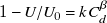 $1-U/U_0=kC_d^\beta$
, with
$1-U/U_0=kC_d^\beta$
, with $\beta$
estimated by ordinary least squares and uncertainty quantified by a block bootstrap that resamples full days. For each resample we recompute the case means and refit
$\beta$
estimated by ordinary least squares and uncertainty quantified by a block bootstrap that resamples full days. For each resample we recompute the case means and refit $(k,\beta )$
. The daily-block result gives
$(k,\beta )$
. The daily-block result gives $\beta =1.02$
with a 95 % confidence interval (CI) of
$\beta =1.02$
with a 95 % confidence interval (CI) of $[0.93,1.18]$
. A linear-scaling
$[0.93,1.18]$
. A linear-scaling $(\beta =1)$
reference thus lies within the fit’s 95 % bootstrap band, supporting an approximately linear dependence over a wide range of
$(\beta =1)$
reference thus lies within the fit’s 95 % bootstrap band, supporting an approximately linear dependence over a wide range of $C_d$
, with larger relative uncertainty at the weakest-drag cases where the deficit approaches the model’s sensitivity limit.
$C_d$
, with larger relative uncertainty at the weakest-drag cases where the deficit approaches the model’s sensitivity limit.
This near-linear behaviour can be interpreted from a perturbation perspective. Let $\delta U = U_0 - U$
denote the hub-height wind-speed deficit relative to the baseline. In the baseline momentum balance, the large-scale pressure gradient is effectively fixed by the lateral forcing and nudging, so differences across cases arise primarily from the added turbine drag. The drag introduces an additional sink of order
$\delta U = U_0 - U$
denote the hub-height wind-speed deficit relative to the baseline. In the baseline momentum balance, the large-scale pressure gradient is effectively fixed by the lateral forcing and nudging, so differences across cases arise primarily from the added turbine drag. The drag introduces an additional sink of order $C_d U_0^2$
, and when this term is small relative to the background balance, the perturbation velocity responds linearly to the forcing. Normalising gives
$C_d U_0^2$
, and when this term is small relative to the background balance, the perturbation velocity responds linearly to the forcing. Normalising gives $\delta U / U_0 \sim C_d U_0$
with the symbol
$\delta U / U_0 \sim C_d U_0$
with the symbol $\sim$
being the scaling equivalence, so the normalised deficit scales almost linearly with
$\sim$
being the scaling equivalence, so the normalised deficit scales almost linearly with $C_d$
for a given background wind speed. Because
$C_d$
for a given background wind speed. Because $U_0$
varies only modestly across cases, the averaged response collapses onto a near-linear dependence, consistent with results in figure 3.
$U_0$
varies only modestly across cases, the averaged response collapses onto a near-linear dependence, consistent with results in figure 3.
This near-linear scaling also has an important dynamical implication: it indicates that wind-farm forcing remains in the perturbative regime of the coupled atmosphere–ocean system, rather than driving a fundamentally different balance. The drag coefficient serves as a prescribed control parameter that systematically varies the strength of momentum extraction, enabling exploration of the coupled system response across a wide range of forcing magnitudes.
Together, these results confirm that this GTD model captures the leading-order effect of momentum extraction in a physically consistent manner. The scaling provides a compact description of wind-farm-induced wind-speed reduction and establishes a useful control parameter for analysing the spatial and temporal extent of the coupled atmospheric and oceanic response.
Hub-height normalised wind-speed deficit $(1-U/U_0)$
versus hub-height turbine drag
$(1-U/U_0)$
versus hub-height turbine drag $C_d$
. Symbols (GTD-1 to GTD-10) are 30-day time averages; vertical bars are 95 % daily-block bootstrap CIs. Dashed line: power-law fit as
$C_d$
. Symbols (GTD-1 to GTD-10) are 30-day time averages; vertical bars are 95 % daily-block bootstrap CIs. Dashed line: power-law fit as $(1-U/U_0)\sim C_d^{1.02}$
; shaded band: 95 % bootstrap interval of the fit; grey dash–dot: linear scaling.
$(1-U/U_0)\sim C_d^{1.02}$
; shaded band: 95 % bootstrap interval of the fit; grey dash–dot: linear scaling.

Time-averaged horizontal wind-speed difference (GTD minus baseline) over the California Coast. The orange box denotes the Morro Bay lease area, and the blue outline shows the expanded zone, defined as a $7\times$
enlargement in both directions to capture downwind turbine wake effects.
$7\times$
enlargement in both directions to capture downwind turbine wake effects.

3.2. Extent of wind-farm influence zone
Turbine-induced wakes extend beyond the prescribed drag region, so a broader diagnostic is required to capture their spatial footprint. We therefore introduce two nested regions. The first is an expanded zone, defined as a rectangle centred on the Morro Bay lease area with side lengths seven times the original dimensions in each direction. This conservative construction ensures that all wind-farm-induced anomalies are contained within the analysis domain, while the surrounding flow remains essentially unperturbed.
Figure 5 illustrates why such an expanded domain is required. Shown are month-mean near-surface wind-speed differences (GTD minus baseline) for representative cases. For weak drag (e.g. GTD-3) the perturbation remains confined near the lease area and is barely distinguishable from background variability. At GTD-5, a clear wake signature emerges, extending well downstream, and by GTD-7 and GTD-9 the wake intensifies and broadens, with deficits approaching 1 m s $^{-1}$
. These maps demonstrate that the wake footprint extends far beyond the lease boundaries and motivate the need for an objective diagnostic of the affected region. Small wind-speed differences are also visible far from the lease area in figure 5; their magnitude does not increase systematically from GTD-1 to GTD-10, and we therefore interpret them as background noise of the coupled simulation rather than a wind-farm signal.
$^{-1}$
. These maps demonstrate that the wake footprint extends far beyond the lease boundaries and motivate the need for an objective diagnostic of the affected region. Small wind-speed differences are also visible far from the lease area in figure 5; their magnitude does not increase systematically from GTD-1 to GTD-10, and we therefore interpret them as background noise of the coupled simulation rather than a wind-farm signal.
Within the expanded zone we then identify the influence zone, representing the contiguous area significantly affected by turbine drag. For each case, we compute the monthly mean near-surface wind speed, taken at 9 m above sea level (the lowest grid level in the model), relative to the baseline, and mask land points. We focus on near-surface winds rather than hub-height winds, since this field directly controls the surface stress that couples to the ocean. Ocean grid cells where the deficit exceeds a fixed threshold, taken as $10\,\%$
of the baseline mean wind speed over the expanded zone, are flagged as affected. The influence-zone boundary is then defined as the convex hull enclosing all affected points. This procedure yields an objective contour that visualises and quantifies the realistic extent of the wake. Cases with fewer than three affected points are deemed to have no detectable influence zone.
$10\,\%$
of the baseline mean wind speed over the expanded zone, are flagged as affected. The influence-zone boundary is then defined as the convex hull enclosing all affected points. This procedure yields an objective contour that visualises and quantifies the realistic extent of the wake. Cases with fewer than three affected points are deemed to have no detectable influence zone.
Figure 6a shows the influence-zone boundaries for GTD-5 to GTD-10. By construction of the $10\,\%$
criterion, no influence zone is detected for GTD-1 to GTD-4. For moderate drag (GTD-5 to GTD-7), the zones remain compact near the Morro Bay lease area, whereas for stronger drag (GTD-8 to GTD-10) they expand downstream and cover areas 2–3 times larger than the lease itself. This behaviour is consistent with the near-linear scaling of wind-speed deficit in figure 4, indicating that drag magnitude controls both the intensity of the local wind-speed reduction and the spatial extent of the wake.
$10\,\%$
criterion, no influence zone is detected for GTD-1 to GTD-4. For moderate drag (GTD-5 to GTD-7), the zones remain compact near the Morro Bay lease area, whereas for stronger drag (GTD-8 to GTD-10) they expand downstream and cover areas 2–3 times larger than the lease itself. This behaviour is consistent with the near-linear scaling of wind-speed deficit in figure 4, indicating that drag magnitude controls both the intensity of the local wind-speed reduction and the spatial extent of the wake.
Influence zones associated with varying drag strength. Panel ( $a$
) shows near-surface horizontal wind speed (m s
$a$
) shows near-surface horizontal wind speed (m s $^{-1}$
, shading) in the baseline case, with contours enclosing convex regions where the wind-speed reduction exceeds 10 % of the local mean within the expanded domain, shown for GTD-5 to GTD-10. The grey dashed contour indicates the wind-farm region. Panel (
$^{-1}$
, shading) in the baseline case, with contours enclosing convex regions where the wind-speed reduction exceeds 10 % of the local mean within the expanded domain, shown for GTD-5 to GTD-10. The grey dashed contour indicates the wind-farm region. Panel ( $b$
) shows the dependence of the diagnosed influence-zone area on drag strength. No influence zone is detected for GTD-1 to GTD-4, whereas finite areas appear from GTD-5 onwards and increase systematically with drag strength.
$b$
) shows the dependence of the diagnosed influence-zone area on drag strength. No influence zone is detected for GTD-1 to GTD-4, whereas finite areas appear from GTD-5 onwards and increase systematically with drag strength.

Figure 6 Long description
Panel A: A contour plot shows near-surface horizontal wind speed in meters per second, with shading indicating wind speed and contours enclosing regions where wind-speed reduction exceeds 10 percent of the local mean. The contours are shown for GTD-5 to GTD-10, with a grey dashed contour indicating the wind-farm region. Panel B: A line graph shows the dependence of the diagnosed influence-zone area in square kilometers on drag strength. The x-axis represents GTD case numbers from 1 to 10, and the y-axis represents the influence zone size. No influence zone is detected for GTD-1 to GTD-4, whereas finite areas appear from GTD-5 onwards and increase systematically with drag strength.
Figure 6b quantifies these changes by plotting the influence-zone area across drag cases. The results confirm the transition: no zones for GTD-1 to GTD-4, compact zones for GTD-5 to GTD-7 and rapid growth with downstream extension for GTD-8 to GTD-10. Taken together, these results demonstrate that turbine drag governs the onset and progressive downstream expansion of near-surface wind-speed deficits, thereby establishing the influence zone as a physically interpretable diagnostic of atmospheric modification. When the hub-height wind-speed deficit is averaged over a region that includes both the lease area and its downstream wake, the power-law fit of figure 4 yields a near-linear scaling ( $\beta = 0.91$
, 95 % bootstrap CI [0.82, 1.08]), statistically consistent with linear scaling and with the lease-area result (
$\beta = 0.91$
, 95 % bootstrap CI [0.82, 1.08]), statistically consistent with linear scaling and with the lease-area result ( $\beta = 1.02$
). The mildly shallower exponent reflects dilution by the wake region, where no explicit drag force is imposed and the deficit decays downstream. Details of this auxiliary fit and the corresponding figure are provided in the Supplementary Material (Section S5, figure S2).
$\beta = 1.02$
). The mildly shallower exponent reflects dilution by the wake region, where no explicit drag force is imposed and the deficit decays downstream. Details of this auxiliary fit and the corresponding figure are provided in the Supplementary Material (Section S5, figure S2).
3.3. Sea-surface-temperature response
The SST provides a useful proxy for coastal upwelling, as colder subsurface water is brought into the surface layer during upwelling events (García-Reyes & Largier Reference García-Reyes and Largier2012; Benazzouz et al. Reference Benazzouz, Mordane, Orbi, Chagdali, Hilmi, Atillah, Pelegrí and Hervé2014; Gutiérrez-Guerra et al. Reference Gutiérrez-Guerra, Pérez-Hernández and Vélez-Belchí2024). Here, we analyse SST anomalies, defined as the difference between each GTD case and the baseline, to isolate the oceanic response to wind-farm forcing. The adjustment of SST is more complex than the near-surface wind field: reduced winds alter surface stress on the ocean and Ekman transport in the ocean, which in turn modify vertical exchange and are ultimately expressed as SST anomalies. Although vertical velocity is a more direct diagnostic of upwelling, SST is considered first because it is readily measurable and provides an interpretable surface expression of the coupled response. The subsurface vertical velocity response is discussed in Section 3.5.
Figure 7 shows the spatial standard deviation of SST anomalies for three consecutive 10-day averaging windows, computed separately for the expanded zone (blue region in figure 5) and the background zone, defined as the complementary ocean area outside the expanded zone. This metric measures the amplitude of spatial variability of SST anomalies within each domain. In the expanded zone, the first 10-day averages highlight a bifurcation between weak and strong drag cases: variability, shown by the blue solid line, increases with drag strength and a threshold-like transition occurs around GTD-4 to GTD-5. The GTD cases 1–4 show weak signal, while from GTD-5 onward the variability rises abruptly. This bifurcation indicates that only sufficiently strong forcing projects coherently onto the mixed layer. By contrast, the background zone remains statistically unchanged across different drag cases, confirming that the wake-induced signal is confined to the vicinity of the wind farm. As the averaging window moves from 1–10 days to 21–30 days, the standard deviation grows, reflecting the accumulation of anomalies through temporal accumulation and interaction with background mesoscale circulation. Despite this amplification, the separation between weak and strong drag cases remains clear across all windows, showing that the onset of SST variability around GTD-5 is robust to averaging period.
Spatial standard deviation of time-averaged SST anomalies (GTD minus baseline) for three consecutive 10-day windows. Results are shown for the expanded zone (wake region) and a background zone outside the expanded domain, defined in Section 3.3.

3.4. The EOF-based quantification and structure of SST dipole response
The SST dipole response across GTD cases. Panel ( $a$
) shows dipole strength, defined as the projection of SST anomalies onto the leading EOF mode, plotted against GTD case number. Panel (
$a$
) shows dipole strength, defined as the projection of SST anomalies onto the leading EOF mode, plotted against GTD case number. Panel ( $b$
) shows spatial structure of the leading EOF mode, showing a canonical dipole aligned with the mean wind. Panels (
$b$
) shows spatial structure of the leading EOF mode, showing a canonical dipole aligned with the mean wind. Panels ( $c$
–
$c$
– $h$
) show comparisons of full SST anomaly fields and their EOF reconstructions for selected cases (GTD-1, GTD-7, GTD-10), illustrating the emergence and intensification of the dipole with increasing drag.
$h$
) show comparisons of full SST anomaly fields and their EOF reconstructions for selected cases (GTD-1, GTD-7, GTD-10), illustrating the emergence and intensification of the dipole with increasing drag.

To characterise the dominant SST response pattern across simulations, we apply an EOF decomposition to the SST anomaly fields, extracting the leading coherent structure and a scalar amplitude for each case to compare dipole strength across the drag spectrum. For each GTD case, the 10-day mean SST field, $\overline {T}_i(x,y)$
, was computed and compared with the corresponding baseline mean,
$\overline {T}_i(x,y)$
, was computed and compared with the corresponding baseline mean, $\overline {T}_{\mathrm{base}}(x,y)$
. The SST anomaly is
$\overline {T}_{\mathrm{base}}(x,y)$
. The SST anomaly is
 \begin{equation} \Delta T_i(x,y)=\overline {T}_i(x,y)-\overline {T}_{\mathrm{base}}(x,y). \end{equation}
The analysis is restricted to ocean points within the expanded zone surrounding the Morro Bay lease area. Let $\boldsymbol{x}_i\in \mathbb{R}^N$
collect
$\boldsymbol{x}_i\in \mathbb{R}^N$
collect $\Delta T_i$
at these
$\Delta T_i$
at these $N$
ocean grid points, and assemble
$N$
ocean grid points, and assemble $\mathbf{X}\in \mathbb{R}^{10\times N}$
with rows
$\mathbf{X}\in \mathbb{R}^{10\times N}$
with rows $\boldsymbol{x}_i$
. An EOF of
$\boldsymbol{x}_i$
. An EOF of $\mathbf{X}$
(via singular value decomposition (SVD)) yields the leading spatial mode
$\mathbf{X}$
(via singular value decomposition (SVD)) yields the leading spatial mode $\boldsymbol{\phi }_1$
with unit
$\boldsymbol{\phi }_1$
with unit $L^2$
norm,
$L^2$
norm, $\|\boldsymbol{\phi }_1\|_2=1$
. The least-squares coefficient for case
$\|\boldsymbol{\phi }_1\|_2=1$
. The least-squares coefficient for case $i$
is
$i$
is $z_i=\boldsymbol{x}_i^\top \boldsymbol{\phi }_1$
. For physical interpretability we define a peak-like amplitude for each case
$z_i=\boldsymbol{x}_i^\top \boldsymbol{\phi }_1$
. For physical interpretability we define a peak-like amplitude for each case
 \begin{equation} \alpha _i = z_i\,\|\boldsymbol{\phi }_1\|_{\infty } = \left (\sum _{j=1}^{N}\Delta T_i^{(j)}\,\phi _1^{(j)}\right )\,\|\boldsymbol{\phi }_1\|_{\infty }, \end{equation}
which has units of temperature and equals the maximum magnitude of the rank-1 reconstruction $\widehat {\Delta T}_i^{(1)}(x,y)=\alpha _i\,\boldsymbol{\phi }_1(x,y)/\|\boldsymbol{\phi }_1\|_{\infty }$
; hence
$\widehat {\Delta T}_i^{(1)}(x,y)=\alpha _i\,\boldsymbol{\phi }_1(x,y)/\|\boldsymbol{\phi }_1\|_{\infty }$
; hence $ \max _{x,y}|\widehat {\Delta T}_i^{(1)}|=|\alpha _i|$
.
$ \max _{x,y}|\widehat {\Delta T}_i^{(1)}|=|\alpha _i|$
.
The dipole strength $\alpha _i$
is shown in figure 8a as a function of drag intensity. For GTD-1 to GTD-4, the values remain close to zero and do not vary with drag, indicating that weak perturbations are insufficient to produce a coherent oceanic response. Beyond GTD-5 when the wind-speed deficit exceeds approximately 5 %, as shown in figure 4, the dipole strength increases systematically with drag. This bifurcation-like transition contrasts with the smoother scaling of wind-speed deficit, and reflects the greater complexity of SST adjustment, which arises through modified surface stress, Ekman transport and vertical exchange.
$\alpha _i$
is shown in figure 8a as a function of drag intensity. For GTD-1 to GTD-4, the values remain close to zero and do not vary with drag, indicating that weak perturbations are insufficient to produce a coherent oceanic response. Beyond GTD-5 when the wind-speed deficit exceeds approximately 5 %, as shown in figure 4, the dipole strength increases systematically with drag. This bifurcation-like transition contrasts with the smoother scaling of wind-speed deficit, and reflects the greater complexity of SST adjustment, which arises through modified surface stress, Ekman transport and vertical exchange.
The leading EOF mode, shown in figure 8b, reveals a coherent dipole pattern aligned with the prevailing wind. The dipole reflects the wind-aligned ocean response to a finite-area reduction in wind stress. Weakened stress reduces vertical mixing in the upper ocean, producing a shallower mixed layer and suppressed upward motion within the wake, with compensating enhancements in adjacent regions (Section 3.5; figure 9). The resulting horizontal redistribution of vertical exchange is consistent with the opposite-sign SST anomalies on the two flanks of the wake. Wake-induced SST warming and mixed-layer shoaling under reduced wind stress have recently been reported by Seo et al. (Reference Seo, Sauvage, Renkl, Lundquist and Kirincich2025) for fully coupled simulations on the seasonally stratified US East Coast. The systematic onset of the dipole beyond GTD-5 coincides with the wind-speed deficit exceeding $\sim 5\,\%$
(figure 4). Panels (
$\sim 5\,\%$
(figure 4). Panels ( $c$
–
$c$
– $h$
) compare the full SST anomaly fields with their EOF reconstructions for selected cases (GTD-1, GTD-7, GTD-10). The case GTD-1 exhibits weak, incoherent anomalies, whereas GTD-10 is strongly aligned with the dipole mode, and the projection reproduces the anomaly structure with high fidelity.
$h$
) compare the full SST anomaly fields with their EOF reconstructions for selected cases (GTD-1, GTD-7, GTD-10). The case GTD-1 exhibits weak, incoherent anomalies, whereas GTD-10 is strongly aligned with the dipole mode, and the projection reproduces the anomaly structure with high fidelity.
To quantify how well the leading mode represents the SST anomaly in the expanded zone, we evaluate the fraction of variance captured by its projection. For each case GTD- $i$
, let
$i$
, let $\boldsymbol{x}_i$
denote the vectorised anomaly temperature field and
$\boldsymbol{x}_i$
denote the vectorised anomaly temperature field and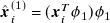 $\hat {\boldsymbol x}_i^{(1)}=(\boldsymbol{x}_i^T\phi _1)\phi _1$
its rank-1 approximation. We define
$\hat {\boldsymbol x}_i^{(1)}=(\boldsymbol{x}_i^T\phi _1)\phi _1$
its rank-1 approximation. We define
 \begin{align} R_i^2=1-\frac {\Vert \boldsymbol x_i -\hat {\boldsymbol x}_i^{(1)}\Vert _2^2}{\Vert \boldsymbol x_i\Vert ^2_2}, \end{align}
the fraction of anomaly variance carried by the leading-order mode. Across the ensemble of all GTD cases, the leading mode explains 87 % of the variance. The value of $R_i^2$
increases with drag: under weak forcing the anomaly is largely unorganised and the dipole accounts for a small fraction (
$R_i^2$
increases with drag: under weak forcing the anomaly is largely unorganised and the dipole accounts for a small fraction ( $R_i^2\sim [22\,\%,43\,\%]$
for GTD-1 to GTD-4), whereas stronger forcing concentrates variance into the wind-aligned dipole pattern (
$R_i^2\sim [22\,\%,43\,\%]$
for GTD-1 to GTD-4), whereas stronger forcing concentrates variance into the wind-aligned dipole pattern ( $R_i^2\sim [92\,\%,97\,\%]$
for GTD-8 to GTD-10). This behaviour is consistent with a forced oceanic Ekman-upwelling response emerging once turbine-induced wind-stress perturbations exceed background mesoscale variability on multi-day time scales.
$R_i^2\sim [92\,\%,97\,\%]$
for GTD-8 to GTD-10). This behaviour is consistent with a forced oceanic Ekman-upwelling response emerging once turbine-induced wind-stress perturbations exceed background mesoscale variability on multi-day time scales.
The EOF analysis therefore provides a unifying framework across all drag cases: it isolates the canonical dipole response, quantifies its amplitude with a single scalar diagnostic and reveals the sensitivity of ocean adjustment to wind-farm forcing on multi-day time scales. This approach demonstrates how systematic variation of turbine drag translates into threshold behaviour and progressive strengthening of the SST dipole.
The SST response is diagnosed from its spatial structure, a wind-aligned dipole (figure 8) and from its scaling with imposed drag. We interpret this pattern as consistent with an oceanic response to wind-stress perturbations, in which modified Ekman transport and vertical mixing alter the surface-temperature field. Through a mixed-layer temperature budget analysis for the seasonally stratified Mid-Atlantic Bight, Seo et al. (Reference Seo, Sauvage, Renkl, Lundquist and Kirincich2025) attributed the wake-induced SST warming to ocean-side processes. They found that weaker wind stress reduces upper-ocean vertical mixing, and that a shoaling mixed layer entrains less cold subsurface water. A corresponding causal attribution for the present configuration is beyond the scope of the present work.
3.5. Subsurface ocean response: mixed-layer and vertical motion
Anomalies of MLD ( $a$
–
$a$
– $c$
) and vertical velocity at the MLD base (
$c$
) and vertical velocity at the MLD base ( $d$
–
$d$
– $f$
) for three drag intensities (GTD-1, GTD-7, GTD-10) relative to the baseline. Negative MLD anomalies indicate shoaling within the wake, while vertical velocity anomalies show suppression of upward motion with compensating enhancements nearby. Patterns intensify systematically with drag.
$f$
) for three drag intensities (GTD-1, GTD-7, GTD-10) relative to the baseline. Negative MLD anomalies indicate shoaling within the wake, while vertical velocity anomalies show suppression of upward motion with compensating enhancements nearby. Patterns intensify systematically with drag.

Figure 9 Long description
The image contains six heatmap panels showing anomalies in mixed layer depth (MLD) and vertical velocity at the MLD base for three drag intensities (GTD-1, GTD-7, GTD-10) relative to a baseline. Panel A, B, and C show the anomalies of MLD for GTD-1, GTD-7, and GTD-10 respectively. Panel D, E, and F show the anomalies of vertical velocity for GTD-1, GTD-7, and GTD-10 respectively. Each panel has latitude on the vertical axis and longitude on the horizontal axis. The color scale on the right indicates the magnitude of the anomalies, with green to red for MLD and blue to red for vertical velocity. Negative MLD anomalies indicate shoaling within the wake, while vertical velocity anomalies show suppression of upward motion with compensating enhancements nearby. Patterns intensify systematically with drag.
In Section 3.4 we examined SST anomalies under different wind-farm-induced drag forcings. While SST provides a conveniently measurable surface proxy, it reflects multiple processes and does not uniquely isolate the vertical exchange that sustains ocean upwelling. Here, we analyse the subsurface ocean response, including MLD and vertical motion. The upper ocean consists of a near-surface mixed layer overlying a stratified interior. Within the mixed layer, temperature and density are nearly uniform with depth, while below it stratification dominates and suppresses vertical exchange. The MLD marks this transition and provides a natural reference for diagnosing upwelling (e.g. Jacox et al. Reference Jacox, Edwards, Hazen and Bograd2018). The vertical velocity at the MLD base directly indicates vertical transport into the mixed layer. Together these diagnostics characterise the subsurface processes that determine the strength of coastal upwelling.
Although MLD and especially vertical velocity are difficult to measure in the field, they can be computed explicitly in numerical simulations, enabling a systematic exploration of their response to wind-farm-induced forcing. Here, the MLD is defined as the depth at which the vertical density difference exceeds 0.03 kg m $^{-3}$
below ocean surface (de Boyer Montégut et al. Reference de Boyer Montégut, Madec, Fischer, Lazar and Iudicone2004). This criterion is applied to vertical density profiles from ROMS to obtain a time- and space-dependent MLD field, which is then used as the reference depth for sampling vertical velocity across cases.
$^{-3}$
below ocean surface (de Boyer Montégut et al. Reference de Boyer Montégut, Madec, Fischer, Lazar and Iudicone2004). This criterion is applied to vertical density profiles from ROMS to obtain a time- and space-dependent MLD field, which is then used as the reference depth for sampling vertical velocity across cases.
The MLD and vertical velocity at the mixed-layer base are computed from the ROMS output, which contains grid-scale fluctuations that could weaken the large-scale wind-farm-induced signal. To recover the underlying response of interest, we first smooth each anomaly field with a Gaussian filter ( $\sigma = 10$
grid points, approximately
$\sigma = 10$
grid points, approximately $10$
km) to damp grid-scale noise while retaining coherent wake structures. We then average the smoothed fields over the 30-day analysis window to reduce short-term transients. This two-step strategy reveals the mesoscale, quasi-steady subsurface response to turbine-induced drag.
$10$
km) to damp grid-scale noise while retaining coherent wake structures. We then average the smoothed fields over the 30-day analysis window to reduce short-term transients. This two-step strategy reveals the mesoscale, quasi-steady subsurface response to turbine-induced drag.
Figure 9 shows the effect of wind-farm drag on MLD and vertical velocity at the mixed-layer base for three representative cases (GTD-1, GTD-7, GTD-10). Panels ( $a$
–
$a$
– $c$
) demonstrate that MLD anomalies are centred on the wake and strengthen with drag. For GTD-1, the anomalies are weak and indistinguishable from background variability. At GTD-7, coherent shoaling of order 5–10 m emerges across the lease area and extends downstream. By GTD-10, the shoaling intensifies to approximately 15 m. Panels (
$c$
) demonstrate that MLD anomalies are centred on the wake and strengthen with drag. For GTD-1, the anomalies are weak and indistinguishable from background variability. At GTD-7, coherent shoaling of order 5–10 m emerges across the lease area and extends downstream. By GTD-10, the shoaling intensifies to approximately 15 m. Panels ( $d$
–
$d$
– $f$
) show a parallel response in vertical velocity: GTD-1 exhibits weak signal, GTD-7 displays systematic suppression of upward motion within the wake and GTD-10 shows reductions exceeding
$f$
) show a parallel response in vertical velocity: GTD-1 exhibits weak signal, GTD-7 displays systematic suppression of upward motion within the wake and GTD-10 shows reductions exceeding $-7\times 10^{-5}$
m s
$-7\times 10^{-5}$
m s $^{-1}$
with compensating enhancements in adjacent regions. The consistency between
$^{-1}$
with compensating enhancements in adjacent regions. The consistency between $\Delta$
MLD and
$\Delta$
MLD and $\Delta w$
across drag levels highlights the underlying mechanism: reduced wind stress decreases turbulent mixing and Ekman pumping in the ocean, producing a shallower mixed layer and weaker upwelling. Although surface heat-flux changes can contribute to mixed-layer evolution, the co-variation of
$\Delta w$
across drag levels highlights the underlying mechanism: reduced wind stress decreases turbulent mixing and Ekman pumping in the ocean, producing a shallower mixed layer and weaker upwelling. Although surface heat-flux changes can contribute to mixed-layer evolution, the co-variation of $\Delta \mathrm{MLD}$
and
$\Delta \mathrm{MLD}$
and $\Delta w$
with the imposed drag supports a primarily wind-stress-driven ocean pathway for the SST response. The progression from negligible anomalies at weak drag to pronounced and coherent patterns at strong drag shows that subsurface anomalies strengthen gradually with wind-farm-induced forcing.
$\Delta w$
with the imposed drag supports a primarily wind-stress-driven ocean pathway for the SST response. The progression from negligible anomalies at weak drag to pronounced and coherent patterns at strong drag shows that subsurface anomalies strengthen gradually with wind-farm-induced forcing.
Spatial correlation between MLD and vertical velocity anomalies. Panel ( $a$
) shows correlation time series for GTD-1, GTD-7 and GTD-10 over the 30-day integration. Panel (
$a$
) shows correlation time series for GTD-1, GTD-7 and GTD-10 over the 30-day integration. Panel ( $b$
) shows distribution of correlations across all cases, with boxes showing interquartile ranges and medians. Correlations remain positive across cases, indicating consistent co-variation of mixed-layer shoaling and suppressed upwelling within the wake.
$b$
) shows distribution of correlations across all cases, with boxes showing interquartile ranges and medians. Correlations remain positive across cases, indicating consistent co-variation of mixed-layer shoaling and suppressed upwelling within the wake.

Figure 10 assesses the co-variation between MLD and vertical velocity anomalies within the expanded zone. Panel ( $a$
) shows the time series of the spatial correlation
$a$
) shows the time series of the spatial correlation $R_{\textit{MLD}\text{-}W}$
for three representative cases (GTD-1, GTD-7 and GTD-10). The evolution of
$R_{\textit{MLD}\text{-}W}$
for three representative cases (GTD-1, GTD-7 and GTD-10). The evolution of $R_{\textit{MLD}\text{-}W}$
is broadly similar across cases, with correlations fluctuating around 0.2–0.5. Although earlier discussions show that the amplitudes of
$R_{\textit{MLD}\text{-}W}$
is broadly similar across cases, with correlations fluctuating around 0.2–0.5. Although earlier discussions show that the amplitudes of $\Delta$
MLD and
$\Delta$
MLD and $\Delta w$
grow with drag, their spatial correlation, which is a measure of co-organisation, does not vary systematically with drag. Panel (
$\Delta w$
grow with drag, their spatial correlation, which is a measure of co-organisation, does not vary systematically with drag. Panel ( $b$
) in figure 10 summarises the time-averaged statistics over all GTD cases and confirms this finding. Median values remain positive (approximately
$b$
) in figure 10 summarises the time-averaged statistics over all GTD cases and confirms this finding. Median values remain positive (approximately $0.2$
–
$0.2$
– $0.3$
) with similar interquartile ranges. The correlation statistics remain relatively insensitive to drag intensity, indicating a persistent relation between mixed-layer shoaling and reduced upward velocity.
$0.3$
) with similar interquartile ranges. The correlation statistics remain relatively insensitive to drag intensity, indicating a persistent relation between mixed-layer shoaling and reduced upward velocity.
3.6. Implications for upwelling dynamics
Wind-farm wakes act as localised stress deficits that weaken Ekman transport. In the wind-farm area, the mixed-layer shoals and the upward velocity at its base is reduced; neighbouring regions show compensating increases, consistent with continuity. Vertical transport is therefore redistributed laterally.
These wake effects operate on scales smaller than those set by large-scale atmospheric forcing and coastline geometry, and thus represent a local adjustment embedded within the broader wind-driven coastal upwelling system. The response is conditioned by the background ocean circulation, which evolves on slower time scales than the atmospheric flow. The present study considers successive month-long simulations with systematically varied wind-farm drag; this framework attributes the response directly to drag perturbations but does not represent longer-term variability or slower oceanic adjustment processes.
We adopt a dynamical-systems view, treating the hub-height drag amplitude as the control parameter that organises the coupled atmosphere–ocean adjustment. This framework is general and not tied to a particular month or site. Future research will apply it across seasonal and interannual conditions and assess how month-scale drag-induced environmental adjustments compound over longer time scales to influence regional coastal upwelling.
4. Conclusions
This study examined the coupled atmosphere–ocean response to offshore wind-farm drag using a high-resolution COAWST configuration of the central California coast. Turbines were represented as an idealised, height-varying momentum sink with systematically varied drag intensity, allowing controlled assessment of how wind-farm-induced forcing modifies coastal upwelling dynamics.
The atmospheric response followed a near-linear scaling: hub-height and near-surface wind-speed deficits increased monotonically with drag, and the spatial influence zone expanded progressively downstream. These results demonstrate that the prescribed drag amplitude provides a systematic control parameter for the strength of momentum extraction, with clear effects on both the magnitude and extent of wind-speed reductions. At the ocean surface, SST anomalies revealed a threshold-like response. An EOF decomposition identified a canonical dipole structure aligned with the mean wind: coastal cooling accompanied by warming on the offshore side of the wind farm. The dipole strength remains negligible for weak drag and increases once the wind-speed deficit exceeds approximately 5 %, indicating that only sufficiently strong perturbations project coherently onto the mixed layer. Subsurface diagnostics showed that wind-farm wakes consistently produced shoaling of the mixed layer and suppression of upward velocities within the wind-farm region. Mixed-layer depth and vertical velocity anomalies were positively correlated across all drag cases, confirming the coupled reduction of vertical mixing and upwelling in wake regions. Adjacent compensating motions indicated that the ocean circulation redistributes rather than eliminates vertical exchange.
Overall, the results establish a mechanistic relation between turbine-induced drag and the surface and subsurface structure of coastal upwelling, providing a framework for interpreting wind-farm effects within the broader coastal dynamical system. By isolating first-order dynamical responses in a controlled setting, this work offers a foundation for offshore wind research seeking to quantify and anticipate air–sea feedbacks associated with large-scale wind energy deployment.
Supplementary material
The supplementary material for this article can be found at https://doi.org/10.1017/flo.2026.10059.
Data availability statement
Data will be made available on reasonable request.
Funding statement
This work was performed under the auspices of the U.S. Department of Energy by Lawrence Livermore National Laboratory under contract DE-AC52-07NA27344, National Laboratory of the Rockies under contract No. DE-AC36-08GO28308 and Pacific Northwest National Laboratory under contract DE-AC05-76RL01830. LLNL release number: LLNL-JRNL-2010824. This research was performed using computational resources sponsored by the U.S. Department of Energy’s Office of Critical Minerals and Energy Innovation and located at the National Laboratory of the Rockies. The views expressed in the article do not necessarily represent the views of the DOE or the U.S. Government. The U.S. Government retains and the publisher, by accepting the article for publication, acknowledges that the U.S. Government retains a non-exclusive, paid-up, irrevocable, worldwide licence to publish or reproduce the published form of this work, or allow others to do so, for U.S. Government purposes.
Competing interests
The authors declare no conflicts of interest.
Ethical statement
The research meets all ethical guidelines, including adherence to the legal requirements of the study country.

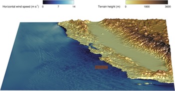
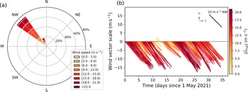
 |U→hub|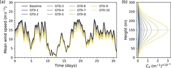
 a
a b
b Cd(z)
Cd(z) Cd=8.6×10⁻⁷m−1
 Cd=3.0×10⁻⁵m−1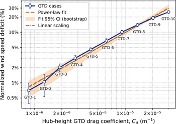
 (1−U/U0)
 Cd
Cd (1−U/U0)∼Cd1.02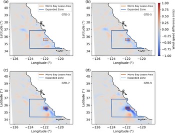
 7×
7×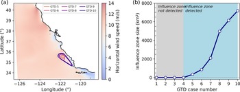
 a
a −1
−1 b
b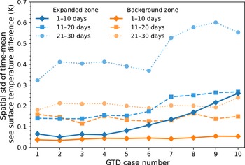

 a
a b
b c
c h
h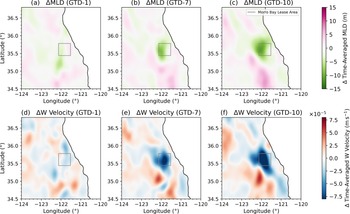
 a
a c
c d
d f
f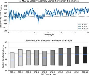
 a
a b
b


 Open access

