






1 Introduction and background
Yeasts are unicellular eukaryotic organisms that have diverse effects on human life. A major negative effect is their ability to colonize implanted medical devices such as catheters, prostheses and stents [Reference Kojic and Darouiche35, Reference Martinez and Fries42]. Yeasts such as Candida albicans (C. albicans) and Candida auris are opportunistic pathogens responsible for up to 44% of severe hospital-acquired infections [Reference Schelenz59], which have mortality rates of between 15% and 35% [Reference Ahmad and Alfouzan2, Reference Pfaller, Andes, Diekema, Horn, Reboli, Rotstein, Franks and Azie53]. Yeasts are infectious because they can invade surrounding tissue [Reference Cullen and Sprague20], thanks, at least in part, to their ability to form hyphae [Reference Boswell and Davidson12] or pseudohyphae [Reference Binder, Sundstrom, Gardner, Jiranek and Oliver9, Reference Gimeno, Ljungdahl, Styles and Fink28]. Therefore, some scientific work on yeasts has focused on understanding cellular behaviours that give rise to macroscopic patterns in pseudohyphal [Reference Li, Green, Tronnolone, Tam, Black, Gardner, Sundstrom, Jiranek and Binder37] or hyphal [Reference Meškauskas, Fricker and Moore43, Reference Meškauskas, McNulty and Moore44] colonies. Much of this work involves the species Saccharomyces cerevisiae (S. cerevisiae), which was the first eukaryotic organism to have its genome fully sequenced [Reference Goffeau29]. Since then, this yeast has become an even more common model organism in cell biology research [Reference Bojsen, Andersen and Regenberg11, Reference Botstein, Chervitz and Cherry13], aiding the understanding of pathogenic yeasts [Reference Berman and Sudbery8] and the behaviour of eukaryotic cells more generally [Reference Botstein, Chervitz and Cherry13].
S. cerevisiae also has uses in the production of food (as reflected by its common name of “baker’s yeast”), medicines [Reference Abid, Waseem, Ali, Ghazanfar, Ali, Elasbali and Alharethi1] and biofuels [Reference Liu, Wang and Nielsen40]. Another common use of yeast is in brewing alcoholic beverages, where optimization of yeast strains is an ongoing area of innovation in wine production [Reference Gardner, Alperstein, Walker, Zhang and Jiranek26, Reference Tek, Sundstrom, Gardner, Oliver and Jiranek64]. Strain optimization increasingly involves bioprospecting, the process of uncovering new strains in natural habitats, as winemakers seek improved quality and fermentation efficiency [Reference Jiranek33]. This continual discovery of new strains motivates ongoing scientific research into understanding differences in growth between yeast species and strains in different experimental conditions.
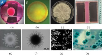
The diversity of yeasts’ effects on life is mirrored by their diversity in modes of growth. Many different growth modes can be reproduced in laboratory experiments, as illustrated in Figure 1. These morphologies are mediated by factors including the yeast species, genetic make up [Reference Reynolds, Jansen, Peng and Fink58], adhesins [Reference Willaert73], nutrient availability [Reference Gimeno, Ljungdahl, Styles and Fink28, Reference Tam, Green, Balasuriya, Tek, Gardner, Sundstrom, Jiranek and Binder60, Reference Tronnolone68, Reference Vulin, Di Meglio, Lindner, Daerr, Murray and Hersen71], quorum sensing [Reference Hogan, Vik and Kolter32, Reference Nickerson, Atkin and Hornby49] and the mechanical properties of the medium on which they are grown [Reference Pietz, John and Thiele54, Reference Pokhrel, Copeland, Hejri, Belpaire, Steinbach, Ng, Hammer and Yunker56]. On soft substrates, yeasts can form colony biofilms that can grow over a 90 mm Petri dish in 1–2 weeks [Reference Andersen, Bojsen, Sørensen, Nielsen, Lisby, Folkesson and Regenberg4, Reference Beauvais, Loussert, Prevost, Verstrepen and Latgé6, Reference Reynolds and Fink57, Reference Reynolds, Jansen, Peng and Fink58, Reference Tam, Green, Balasuriya, Tek, Gardner, Sundstrom, Jiranek and Binder60]. This form of growth is illustrated in Figures 1(a) and 1(d). The distributions of viable and dead cells within these colonies can vary spatially [Reference Plocek, Váchová and Palková55, Reference Váchová, Šťovíček, Hlaváček, Chernyavskiy, Štěpánek, Kubínová and Palková70] and understanding the roles of cell death in yeast colonies is an important subject of research [Reference Čáp, Štěpánek, Harant, Váchová and Palková16, Reference Gourlay, Du and Ayscough30, Reference Palková and Váchová50, Reference Váchová and Palková69]. Yeasts can enter a stationary phase that enables them to survive harsh environments [Reference Minois, Frajnt, Wilson and Vaupel46]. In seemingly opposite behaviour, yeasts can also undergo regulated cell death [Reference Carmona-Gutierrez17], an altruistic process that releases nutrients for future consumption [Reference Netherwood, Tam, Gourlay, Knežević, Gardner, Jiranek, Binder and Green48]. One method for characterizing cell death with colonies is to stain them with Phloxine B [Reference Middelhoven, Broekhuizen and van Eijk45] dye. As illustrated in Figures 1(a) and 1(b), this staining creates darker pink regions indicating elevated cell death. In Figure 1(a), cell death occurs near the centre of the colony. This death is likely to be accidental cell death due to lack of nutrients, similar to a necrotic core. Conversely, in Figure 1(b), cell death is localized in a ring trailing the leading edge. This death may be due to regulated cell death [Reference Netherwood, Tam, Gourlay, Knežević, Gardner, Jiranek, Binder and Green48], which releases nutrients near the leading edge to promote further proliferation. These different forms of cell death highlight yeast’s diversity of growth.
Comparison of yeast colony patterns in different experimental environments. (a) M. magnusii colony biofilm after seven days of growth. Dark regions indicate elevated cell death occurring in a central region resembling a necrotic core, which probably occurs due to accidental cell death (ACD) [Reference Netherwood, Tam, Gourlay, Knežević, Gardner, Jiranek, Binder and Green48]. (b) S. cerevisiae colony biofilm after five days of growth. The red ring indicates elevated cell death, which is probably due to regulated cell death (RCD) [Reference Netherwood, Tam, Gourlay, Knežević, Gardner, Jiranek, Binder and Green48]. (c) S. cerevisiae colony biofilm grown on nutrient-rich soft (0.3%) agar [Reference Reynolds and Fink57, Reference Reynolds, Jansen, Peng and Fink58, Reference Tam, Green, Balasuriya, Tek, Gardner, Sundstrom, Jiranek and Binder60]. (d) Rectangular S. cerevisiae colony biofilm on (0.6%) YPD media. Darker regions indicate elevated cell death compared with lighter regions [Reference Tam, Netherwood, Gardner, Zhang, Gourlay, Jiranek, Binder and Green63]. (e) S. cerevisiae colony grown on YND after 58 days of growth [Reference Tronnolone, Gardner, Sundstrom, Jiranek, Oliver and Binder66]. (f) Filamentous yeast of the S. cerevisiae strain AWRI 796, with 50 $\mu $
m nutrients [Reference Binder, Sundstrom, Gardner, Jiranek and Oliver9]. (g) Intermediate stages of hyphal colony formation in C. albicans [Reference Li, Skivens, Green, Tam, Pentland, Baumann, Gourlay, Binder and Laissue38]. (h) Hyphal M. magnusii colonies grown on a Petri dish with high colony density.
$\mu $
m nutrients [Reference Binder, Sundstrom, Gardner, Jiranek and Oliver9]. (g) Intermediate stages of hyphal colony formation in C. albicans [Reference Li, Skivens, Green, Tam, Pentland, Baumann, Gourlay, Binder and Laissue38]. (h) Hyphal M. magnusii colonies grown on a Petri dish with high colony density.
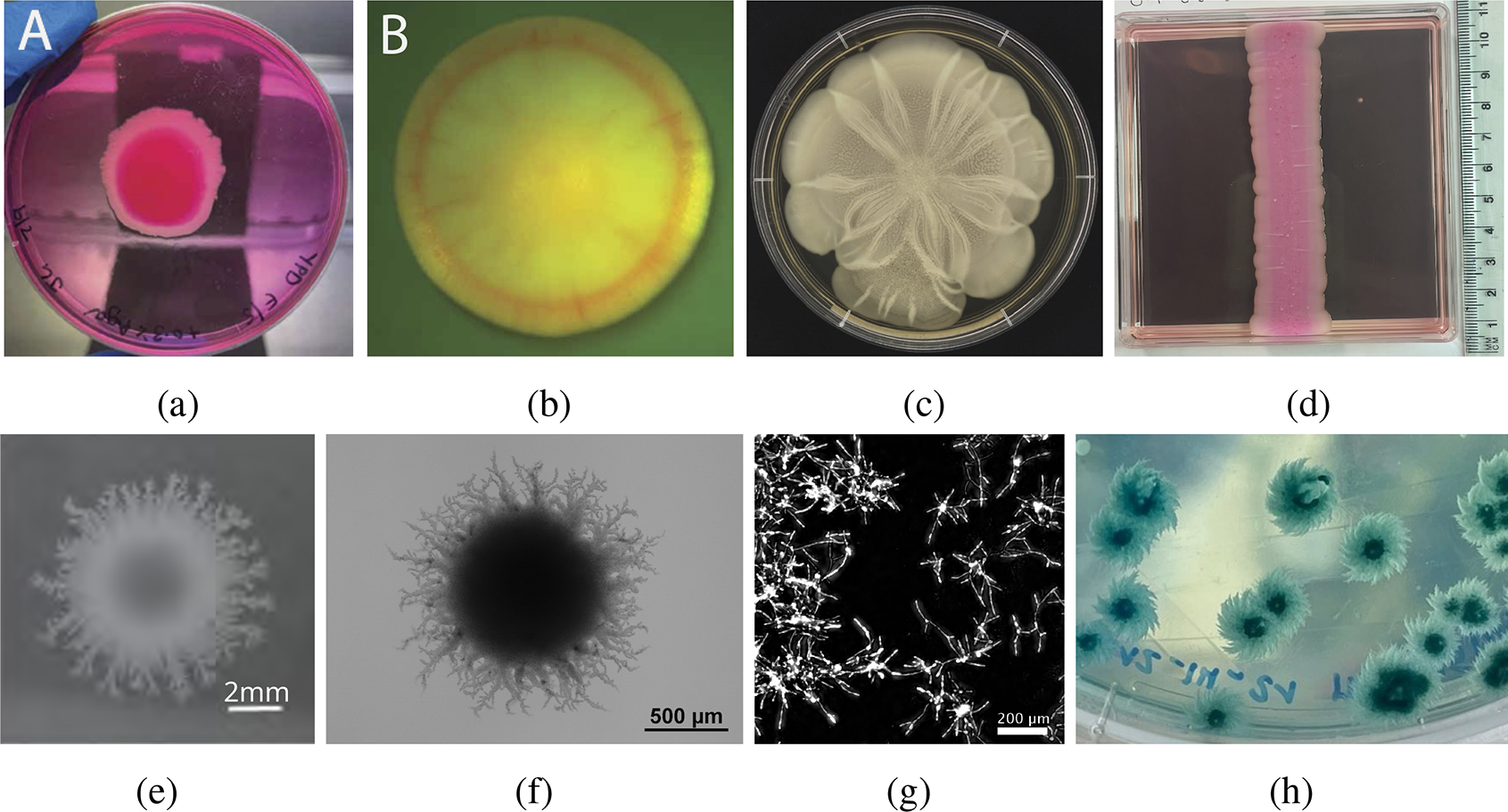
Colony biofilm growth is also influenced by nutrient availability [Reference Tam, Green, Balasuriya, Tek, Gardner, Sundstrom, Jiranek and Binder60, Reference Vulin, Di Meglio, Lindner, Daerr, Murray and Hersen71]. In low-nutrient environments, yeasts form very different morphologies to colony biofilms by producing smaller colonies with nonuniform spatial structure (Figures 1(e) and 1(f)). Interestingly, Tronnolone et al. [Reference Tronnolone68] found that yeasts, which are nonmotile, also cannot respond actively to nutrient gradients. This provided evidence that the nonuniform patterns in Figures 1(e) and 1(f) form due to pseudohyphal growth [Reference Binder, Sundstrom, Gardner, Jiranek and Oliver9, Reference Gimeno, Ljungdahl, Styles and Fink28, Reference Tronnolone, Gardner, Sundstrom, Jiranek, Oliver and Binder66], rather than directed growth in response to environmental gradients. Pseudohyphal growth involves a switch between unipolar and bipolar budding, and the creation of elongated chains of unipolar cells [Reference Gimeno, Ljungdahl, Styles and Fink28], allowing the colony to extend radially to obtain nutrients and to invade agar surfaces. Similar to moulds, yeasts can also form hyphal colonies, where the yeast grows in elongated tubes consisting of multiple cells. Figure 1(g) depicts the early stages of hyphal colony development. Hyphal growth is also affected by many factors, for example, carbon dioxide levels [Reference Pentland, Davis, Mühlschlegel and Gourlay52]. These different colony morphologies illustrate that diversity of outcome is a key characteristic of yeast growth. Given that new strains are being continuously discovered by bioprospecting, there is an incentive for developing robust mathematical modelling and parameter inference methods to understand these new strains. We outline such a procedure in this manuscript.
In search of improved wine strains, we bioprospected a new isolate of Magnusiomyces magnusii (M. magnusii) from the sap of a Tasmanian cider gum tree, Eucalyptus gunnii. Under laboratory conditions, this yeast formed a novel highly ordered spiral morphology (Figure 1(h)). Spiral patterns have been observed during hyphal growth of other fungi [Reference Beever7, Reference Davidson and Gregory21, Reference Madelin, Toomer and Ryan41, Reference Trinci, Saunders, Gosrani and Campbell65]. However, the M. magnusii morphology is distinct from these other fungi and features thicker, more densely packed spirals that form a galaxy-like pattern. We focus on modelling this distinct new morphology. The spiralling morphology in M. magnusii does not occur in all growth environments (data not shown). Spiral formation occurred on plates with high colony density, but not on plates with low colony density. Since colonies on high-density plates face more competition for nutrients from the other colonies, spiral formation appears to represent another adaptation that a yeast has developed in response to a harsh environment.
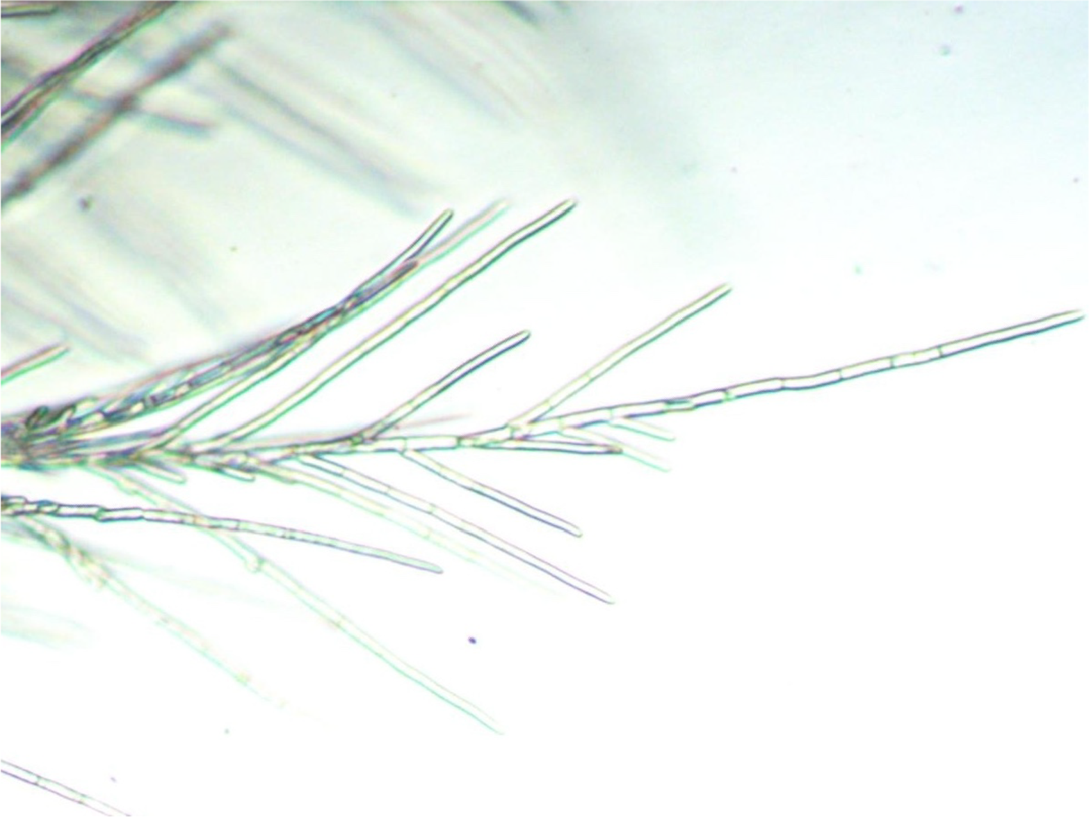
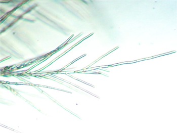
Like S. cerevisiae, M. magnusii colonies create filaments that extend radially from a circular Eden-like [Reference Eden24] region. Unlike S. cerevisiae, where the filaments consist of elongated yeast cells, the main branch of the M. magnusii filament consists of stiff rod-like hyphae [Reference de Hoog, Smith, Kurtzman, Fell and Boekhout22] that are 7–12 $\mu $
m wide. Penicillate secondary branches emerge at acute angles from the main branch, forming a bushy or fan-like arrangement. These thinner secondary branches break apart into arthroconidia, which are rectangular spore-like units 4–7
$\mu $
m wide. Penicillate secondary branches emerge at acute angles from the main branch, forming a bushy or fan-like arrangement. These thinner secondary branches break apart into arthroconidia, which are rectangular spore-like units 4–7 $\mu $
m wide and 10–18
$\mu $
m wide and 10–18 $\mu $
m long (Figure 2). Nonuniform spatial patterns also emerge in hyphal C. albicans colonies [Reference Berman and Sudbery8, Reference Cleary, Mulabagal, Reinhard, Yadev, Murdoch, Thornhill, Lazzell, Monteagudo, Thomas and Saville19, Reference Mohammadi, Leduc, Charette, Barbeau and Vincent47], but they do not exhibit the striking spiral patterns of M. magnusii. The microscale mechanisms that underpin these spiral colonies of M. magnusii remain to be determined.
$\mu $
m long (Figure 2). Nonuniform spatial patterns also emerge in hyphal C. albicans colonies [Reference Berman and Sudbery8, Reference Cleary, Mulabagal, Reinhard, Yadev, Murdoch, Thornhill, Lazzell, Monteagudo, Thomas and Saville19, Reference Mohammadi, Leduc, Charette, Barbeau and Vincent47], but they do not exhibit the striking spiral patterns of M. magnusii. The microscale mechanisms that underpin these spiral colonies of M. magnusii remain to be determined.
Enlarged view of the filamentous region of a hyphal M. magnusii colony from our experiments.
Depending on the type of growth considered, mathematical models of yeast colonies have involved agent-based [Reference Banwarth-Kuhn, Collignon and Sindi5, Reference Li, Green, Tronnolone, Tam, Black, Gardner, Sundstrom, Jiranek and Binder37], reaction–diffusion [Reference Chen, Noorbakhsh, Adams, Samaniego-Evans, Agollah, Nevozhay, Kuzdzal-Fick, Mehta and Balázsi18, Reference Li, Gallo, Binder and Green36, Reference Tam, Green, Balasuriya, Tek, Gardner, Sundstrom, Jiranek and Binder60] and continuum mechanical [Reference Tam, Green, Balasuriya, Tek, Gardner, Sundstrom, Jiranek and Binder61, Reference Tam, Harding, Green, Balasuriya and Binder62] approaches. Owing to the small size of individual M. magnusii colonies, we use an off-lattice agent-based model [Reference Brown, Green, Binder and Osborne14, Reference Browning, McCue, Binny, Plank, Shah and Simpson15, Reference Gallo, Tronnolone, Green and Binder25, Reference Klowss, Browning, Murphy, Carr, Plank, Gunasingh, Haass and Simpson34, Reference Tronnolone, Gardner, Sundstrom, Jiranek, Oliver and Binder66, Reference Wang, Jenner, Salomone, Warne and Drovandi72] to simulate the spiral morphology. Our objective is to understand how cellular behaviour gives rise to colony-scale patterns. Agents in the model represent rod-like segments of fixed size. These segments could represent hyphae, segments of a rod-like hyphal filament, or arthroconidia in a secondary branch. In the model, regular hyphae and arthroconidia can extend from sites located on the sides of the cell, whereas rod-like (filament-forming) hyphae extend end-to-end only, with a prescribed angle between segments. To compare the model with the experiment, we use image processing and Bayesian inference using neural likelihood estimation [Reference Alsing, Charnock, Feeney and Wandelt3, Reference Dyer, Cannon, Farmer and Schmon23, Reference Papamakarios, Sterratt and Murray51]. The shape of the hyphal colony components is mainly governed by the angle between successive hyphal segments. Using realistic parameter estimates, the model can also capture three other distinct colony morphologies formed by M. magnusii grown under different conditions.
2 Yeast growth experiments
An in-house isolate of M. magnusii was used for these experiments. Yeast was cultured in liquid yeast peptone dextrose medium (YPD; ${10}{\text { g L}^{-1}}$
yeast extract,
${10}{\text { g L}^{-1}}$
yeast extract, ${20}{\text { g L}^{-1}}$
peptone,
${20}{\text { g L}^{-1}}$
peptone, ${20}{\text { g L}^{-1}}$
glucose) with 2% agar where solid medium was required. We grew 5 mL yeast cultures for 48 hours in liquid YPD prior to inoculation onto 90 mm round agar plates where a 50
${20}{\text { g L}^{-1}}$
glucose) with 2% agar where solid medium was required. We grew 5 mL yeast cultures for 48 hours in liquid YPD prior to inoculation onto 90 mm round agar plates where a 50 $\mu $
L aliquot diluted to
$\mu $
L aliquot diluted to $4\times 10^{2} \text { cells mL}^{-1}$
(low cell density) or
$4\times 10^{2} \text { cells mL}^{-1}$
(low cell density) or $4\times 10^{3} \text { cells mL}^{-1}$
(high cell density) with phosphate buffered saline was spread plated. Agar plates contained either chemically defined sap medium (CDS;
$4\times 10^{3} \text { cells mL}^{-1}$
(high cell density) with phosphate buffered saline was spread plated. Agar plates contained either chemically defined sap medium (CDS; ${10}{\text { g L}^{-1}}$
yeast extract,
${10}{\text { g L}^{-1}}$
yeast extract, ${20}{\text { g L}^{-1}}$
peptone,
${20}{\text { g L}^{-1}}$
peptone, ${15}{\text { g L}^{-1}}$
glucose,
${15}{\text { g L}^{-1}}$
glucose, ${12}{\text { g L}^{-1}}$
fructose,
${12}{\text { g L}^{-1}}$
fructose, ${9}{\text { g L}^{-1}}$
maltose,
${9}{\text { g L}^{-1}}$
maltose, ${2}{\text { g L}^{-1}}$
glycerol, 1% (v/v) ethanol,
${2}{\text { g L}^{-1}}$
glycerol, 1% (v/v) ethanol, ${1}{\text { g L}^{-1}}$
acetic acid,
${1}{\text { g L}^{-1}}$
acetic acid, ${1}{\text { g L}^{-1}}$
pyruvic acid,
${1}{\text { g L}^{-1}}$
pyruvic acid, ${2}{\text { g L}^{-1}}$
gluconic acid,
${2}{\text { g L}^{-1}}$
gluconic acid, ${0.1}{\text { g L}^{-1}}$
succinic acid) or yeast nitrogen base (YNB; Becton Dickinson; Cat No. 233520), prepared according to the manufacturer’s instructions and with the addition of
${0.1}{\text { g L}^{-1}}$
succinic acid) or yeast nitrogen base (YNB; Becton Dickinson; Cat No. 233520), prepared according to the manufacturer’s instructions and with the addition of ${2}{\text { g L}^{-1}}$
D-glucose and
${2}{\text { g L}^{-1}}$
D-glucose and ${5}{\text { g L}^{-1}}$
ammonium sulfate. Plates were sealed with Parafilm and incubated at 25
${5}{\text { g L}^{-1}}$
ammonium sulfate. Plates were sealed with Parafilm and incubated at 25 $^{\circ }\text {C}$
for 5–10 days. Macroscopic plate images were captured with an Apple iPhone 12 Pro and microscopic imaging with a Leica M-Z FL111 microscope with a Nikon DS-5MC Microscope Camera and Nikon NIS element software or a Carl Zeiss Axiophot Pol Photomicroscope with a Toupcam ultra-high-performance complementary metal–oxide–semiconductor (UCMOS) sensor Microscope Camera and ToupView software.
$^{\circ }\text {C}$
for 5–10 days. Macroscopic plate images were captured with an Apple iPhone 12 Pro and microscopic imaging with a Leica M-Z FL111 microscope with a Nikon DS-5MC Microscope Camera and Nikon NIS element software or a Carl Zeiss Axiophot Pol Photomicroscope with a Toupcam ultra-high-performance complementary metal–oxide–semiconductor (UCMOS) sensor Microscope Camera and ToupView software.
3 Mathematical modelling and parameter inference methods
We aim to develop procedures for mathematical modelling and parameter inference that can apply to a variety of yeast colony morphologies. This section describes off-lattice agent-based modelling and a parameter inference method using sequential neural likelihood estimation. We illustrate these methods on an M. magnusii spiral colony. The biological insight gained includes quantification of the angle between segments in spiral-forming colonies, and understanding of how model parameters, and hence cellular behaviour, differs across experimental conditions.
3.1 Off-lattice agent-based model
Li et al. [Reference Li, Green, Tronnolone, Tam, Black, Gardner, Sundstrom, Jiranek and Binder37] developed a two-dimensional off-lattice agent-based model for filamentous S. cerevisiae colonies, where the filaments consisted of pseudohyphal cells. We adapt this prior model to M. magnusii colonies, which are formed from hyphae. Each hypha consists of many individual cells, forming long and tubular structures much longer than an individual cell, but of similar width. Consequently, hyphae do not proliferate by cellular budding, but still grow and fragment as the colony consumes nutrients. To model growth by hyphal extension, we assume that the colony consists of many rod-like agents as per Figures 2 and 3, and we assume that each agent has the same size. All agents are ellipses with major axis length 22.5 $\mu $
m and minor axis length 7.5
$\mu $
m and minor axis length 7.5 $\mu $
m, giving an aspect ratio of 3 [Reference de Hoog, Smith, Kurtzman, Fell and Boekhout22]. In practice, we represent these ellipses as dodecagons in 2D. These agents can be either regular hyphae, which can produce new hyphal segments at four sites located on their sides at angles of
$\mu $
m, giving an aspect ratio of 3 [Reference de Hoog, Smith, Kurtzman, Fell and Boekhout22]. In practice, we represent these ellipses as dodecagons in 2D. These agents can be either regular hyphae, which can produce new hyphal segments at four sites located on their sides at angles of $\pm 7\pi /16$
radians from the distal poles of the mother hyphae, or filament-forming hyphae, which can only produce a new hyphal segment at one site located at the distal end. To capture the anticlockwise spiralling, hyphal segments in filaments extend at a prescribed acute angle
$\pm 7\pi /16$
radians from the distal poles of the mother hyphae, or filament-forming hyphae, which can only produce a new hyphal segment at one site located at the distal end. To capture the anticlockwise spiralling, hyphal segments in filaments extend at a prescribed acute angle $\theta _p,$
measured anticlockwise from the orientation of the major axis of the segment. This angle is known to be acute [Reference de Hoog, Smith, Kurtzman, Fell and Boekhout22], but has not been previously quantified, and a key contribution of our work is to infer a posterior distribution for this angle. The model features are summarized in Figure 4.
$\theta _p,$
measured anticlockwise from the orientation of the major axis of the segment. This angle is known to be acute [Reference de Hoog, Smith, Kurtzman, Fell and Boekhout22], but has not been previously quantified, and a key contribution of our work is to infer a posterior distribution for this angle. The model features are summarized in Figure 4.
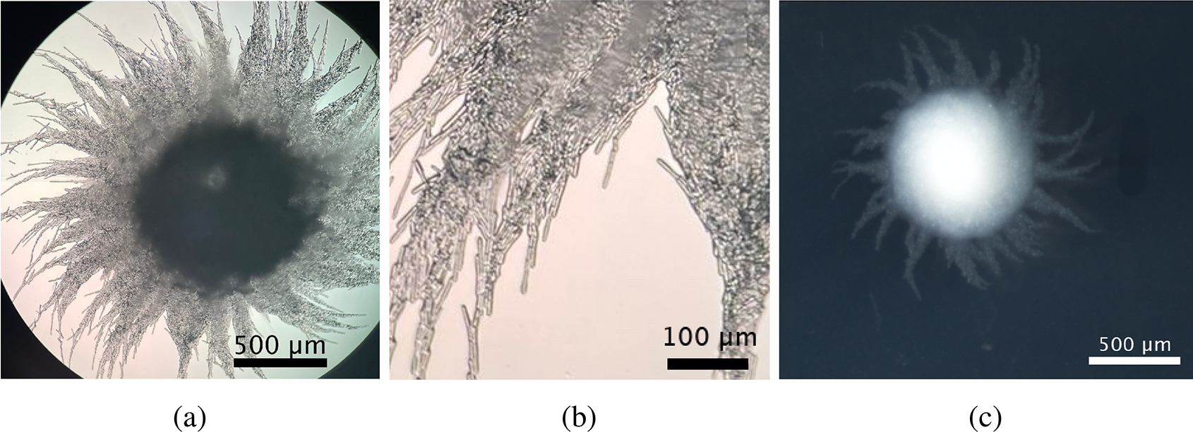
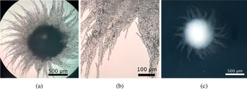
Images of M. magnusii at different magnifications, revealing the microscopic features of the colony structure when grown on CDS medium for 7 days. (a) A colony exhibiting the spiral morphology. (b) Enlarged view of an experimental colony showing hyphae and conidia. (c) Full view of an M. magnusii colony after seven days of growth on YNB with high colony density. This colony is a different experiment to Figures 2, 3(a) and 3(b), and is the colony used when inferring parameters to compare the model and experiment.
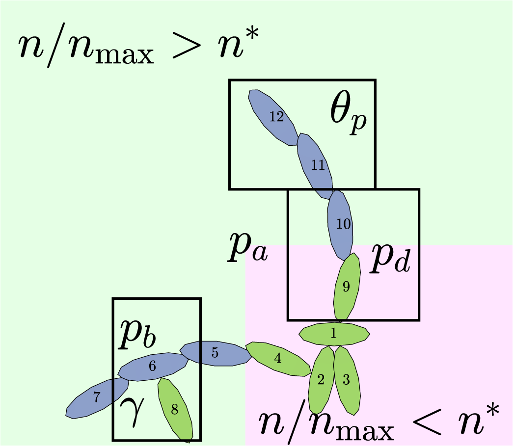
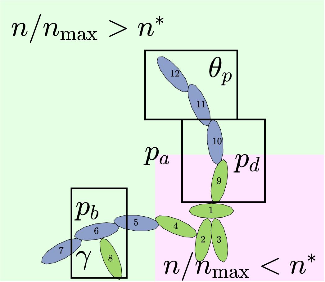
Cellular rules in the modified agent-based model. Regular hyphae that can extend from their sides are shown in green. Filament-forming hyphae that only extend at the angle $\theta _p$
from their distal ends are shown in dark blue. The numbers represent a possible sequence of hyphal growth, starting from hyphal segment 1, that could generate this pattern.
$\theta _p$
from their distal ends are shown in dark blue. The numbers represent a possible sequence of hyphal growth, starting from hyphal segment 1, that could generate this pattern.
We simulate hyphal growth one agent at a time until the colony reaches a prescribed number of agents, $n_{\text {max}}$
, chosen in advance such that the simulation ends when the simulated colony has approximately the same area as an experimental colony. Each step of the simulation involves selecting a hypha to produce a new segment, and proposing the type and location of the new agent. This behaviour depends on six parameters,
$n_{\text {max}}$
, chosen in advance such that the simulation ends when the simulated colony has approximately the same area as an experimental colony. Each step of the simulation involves selecting a hypha to produce a new segment, and proposing the type and location of the new agent. This behaviour depends on six parameters, $\boldsymbol {\theta } = (n^*, p_b, p_d, \gamma , p_a, \theta _p)$
, whose meanings we describe in the following three paragraphs. After proposing the new agent, we implement partial volume exclusion to prevent two agents from occupying the same space. If the centre of a proposed new agent would lie within the boundary of another agent, the hyphal extension event does not occur.
$\boldsymbol {\theta } = (n^*, p_b, p_d, \gamma , p_a, \theta _p)$
, whose meanings we describe in the following three paragraphs. After proposing the new agent, we implement partial volume exclusion to prevent two agents from occupying the same space. If the centre of a proposed new agent would lie within the boundary of another agent, the hyphal extension event does not occur.
On the length scale of M. magnusii experiments, the nutrient concentration is spatially uniform [Reference Tronnolone68]. In the model, we use the existing colony area as a proxy for nutrient availability, such that hyphal filaments can emerge when the colony is sufficiently large. Consequently, we model neither time nor the nutrient concentration explicitly. The parameter $n^* \in [0, 1]$
is the threshold proportion of hyphae, relative to
$n^* \in [0, 1]$
is the threshold proportion of hyphae, relative to $n_{\text {max}}$
, which governs whether filament-forming hyphae can emerge. If the current number of agents in the simulated colony,
$n_{\text {max}}$
, which governs whether filament-forming hyphae can emerge. If the current number of agents in the simulated colony, $n,$
is such that
$n,$
is such that $n < n^*n_{\text {max}}$
, then only regular hyphae that can extend from both ends (shown in green in Figure 4) can be produced. When
$n < n^*n_{\text {max}}$
, then only regular hyphae that can extend from both ends (shown in green in Figure 4) can be produced. When $n> n^*n_{\text {max}}$
, then filament-forming hyphae that extend from one end only (shown in dark blue in Figure 4) can emerge. The threshold
$n> n^*n_{\text {max}}$
, then filament-forming hyphae that extend from one end only (shown in dark blue in Figure 4) can emerge. The threshold $n^*$
thus represents the colony size, relative to
$n^*$
thus represents the colony size, relative to $n_{\text {max}},$
when the environmental conditions (for example, low nutrient availability) required to produce hyphal filaments arise.
$n_{\text {max}},$
when the environmental conditions (for example, low nutrient availability) required to produce hyphal filaments arise.
Once $n/n_{\text {max}}> n^*,$
the other probabilities
$n/n_{\text {max}}> n^*,$
the other probabilities $p_a,\, p_b,\, p_d$
and
$p_a,\, p_b,\, p_d$
and $\gamma $
determine the next hypha to extend, and the type of new agent that is produced. The next agent selected to extend is governed by the probability
$\gamma $
determine the next hypha to extend, and the type of new agent that is produced. The next agent selected to extend is governed by the probability $p_a$
. A regular hypha is selected with probability
$p_a$
. A regular hypha is selected with probability $p_a$
and a filament-forming hypha is selected with probability
$p_a$
and a filament-forming hypha is selected with probability $1-p_a.$
The particular agent to extend is chosen at random from all agents of the relevant type. This assumption represents the hypothesis that initiating filament formation is a colony-level decision.
$1-p_a.$
The particular agent to extend is chosen at random from all agents of the relevant type. This assumption represents the hypothesis that initiating filament formation is a colony-level decision.
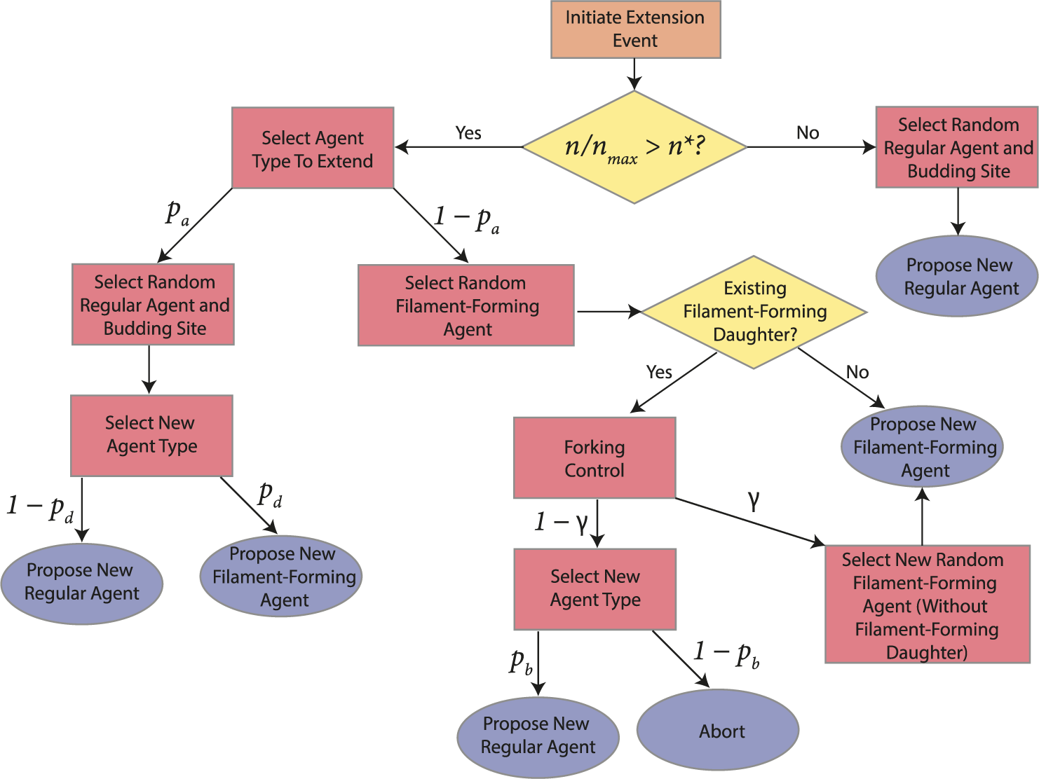
If a regular hypha is selected to extend, then the resulting agent is filament-forming with probability $p_d$
or regular with probability
$p_d$
or regular with probability $1-p_d.$
If a filament-forming hypha is selected, then we first check whether that filament-forming hypha has an existing filament-forming daughter agent. If not, a new filament-forming agent is proposed. If there is an existing filament-forming daughter agent, then the behaviour is governed by
$1-p_d.$
If a filament-forming hypha is selected, then we first check whether that filament-forming hypha has an existing filament-forming daughter agent. If not, a new filament-forming agent is proposed. If there is an existing filament-forming daughter agent, then the behaviour is governed by $p_b$
and
$p_b$
and $\gamma .$
First, with probability
$\gamma .$
First, with probability $\gamma $
, a different filament-forming agent without an existing filament-forming daughter is chosen to extend instead. Larger values of
$\gamma $
, a different filament-forming agent without an existing filament-forming daughter is chosen to extend instead. Larger values of $\gamma $
favour extended chains of individual filament-forming agents and limit the appearance of regular hyphae within these chains. Then, if the agent with the existing filament-forming daughter proceeds to extend (which occurs with probability
$\gamma $
favour extended chains of individual filament-forming agents and limit the appearance of regular hyphae within these chains. Then, if the agent with the existing filament-forming daughter proceeds to extend (which occurs with probability $1-\gamma $
), the proposed new agent will be a regular hyphal segment with probability
$1-\gamma $
), the proposed new agent will be a regular hyphal segment with probability $p_b$
or a filament-forming segment with probability
$p_b$
or a filament-forming segment with probability $1-p_b.$
In the latter scenario, the proliferation event is aborted due to volume exclusion, because filament-forming agents can only extend at one site with orientation
$1-p_b.$
In the latter scenario, the proliferation event is aborted due to volume exclusion, because filament-forming agents can only extend at one site with orientation $\theta _p$
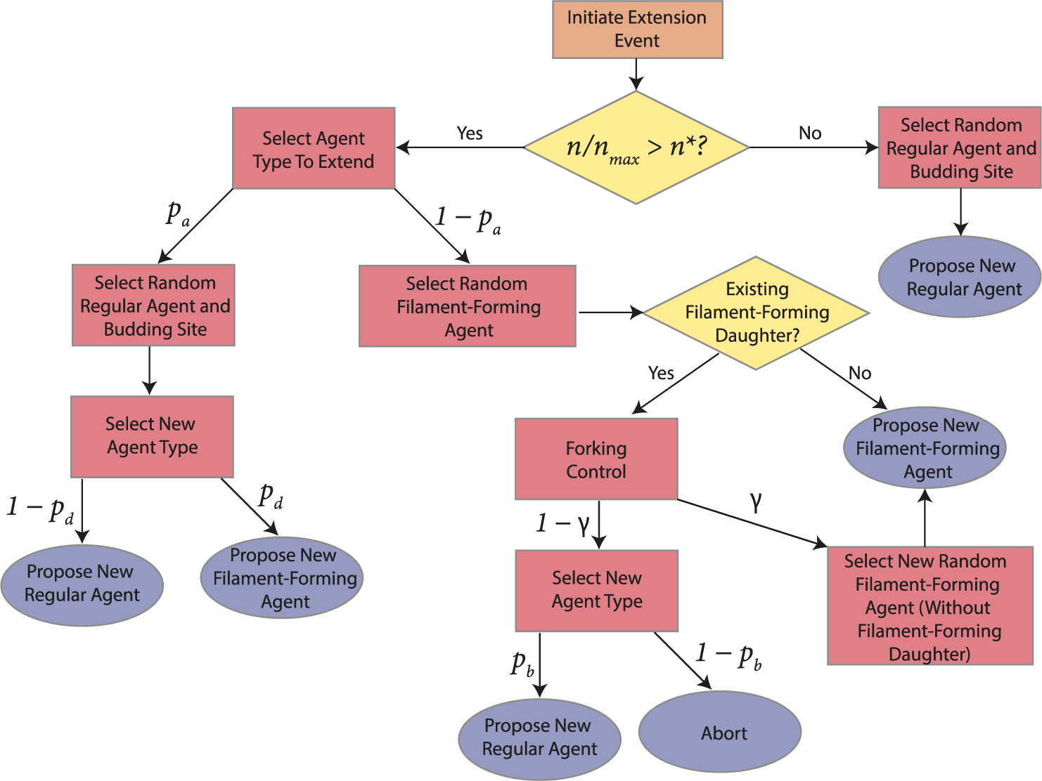
. The flowchart in Figure 5 summarizes steps taken to propose a new agent.
$\theta _p$
. The flowchart in Figure 5 summarizes steps taken to propose a new agent.
Flowchart describing the steps taken to propose a new agent (hyphal segment) in the agent-based model.
Since our agent-based modelling framework is similar to that applied to pseudohyphal growth [Reference Li, Green, Tronnolone, Tam, Black, Gardner, Sundstrom, Jiranek and Binder37], it is adaptable to other yeasts with different forms of growth. Should another yeast species that forms irregularly shaped small colonies be studied, we could readily adapt this model, provided the agent size, budding patterns and experimental colony area (in physical units) are known or assumed in advance. In a previous paper [Reference Li, Green, Tronnolone, Tam, Black, Gardner, Sundstrom, Jiranek and Binder37], we have already applied a similar model to multiple strains of S. cerevisiae grown in different environments. The M. magnusii model presented here is one of many possible model variations and demonstrates how the model can also apply to hyphal growth.
3.2 Image processing and summary statistics
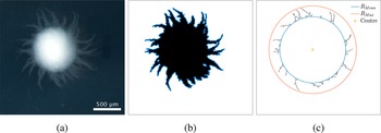
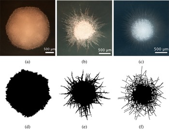
We process experimental photographs and simulation results to quantify the spatial patterns. We convert experimental photographs to binary images using the Tool for Analysis of the Morphology of Microbial Colonies (TAMMiCol) [Reference Tronnolone, Gardner, Sundstrom, Jiranek, Oliver and Binder67], such that black pixels indicate regions occupied by the colony and white pixels indicate unoccupied regions. The binary image for the M. magnusii colony is in Figure 6(b). To enable direct comparison, we save images of the simulated colonies at the same scale and resolution as experimental photographs. We simulate colonies until they attain a target number of agents, which we prescribe. To obtain the target number of agents for the simulations that best fits the experimental data, we used the golden section search to minimize the difference in colony area between the simulated and experimental colonies.
Visualization of the summary statistics used in this paper. (a) Original experimental photograph of a M. magnusii colony with spiral hyphae. (b) Binary image with area overlayed with perimeter (blue). (c) Mean and maximum radii overlayed with the skeletonization of the binary image in panel (b).

For both experimental and simulation results, we define five spatial statistics to characterize morphology: maximum radius ( $R_{\text {max}}$
), mean radius (
$R_{\text {max}}$
), mean radius ( $R_{\text {mean}}$
), filamentous area (
$R_{\text {mean}}$
), filamentous area ( $I_{A_F}$
), branch count (
$I_{A_F}$
), branch count ( $I_B$
) and compactness (
$I_B$
) and compactness ( $I_C$
). The two radii provide two measures of colony size. The maximum radius is the largest distance from the colony centroid to an occupied pixel, and the mean radius is the average distance between the centroid and all pixels on the colony perimeter. The colony centroid is found using Matlab’s regionprops() function. Filamentous area is the number of occupied pixels between the mean and maximum radii, and therefore quantifies the extent of the nonuniform hyphal growth. Branch count quantifies the complexity of the hyphal filament pattern, and is the number of segments identified in a skeletonized image produced using Matlab’s bwmorph() function that lie between the mean and maximum radii. Figure 6(c) provides an example of a skeletonized image. Compactness is the ratio between the colony perimeter and the perimeter of a circle with the same area as the colony, and quantifies the shape irregularity of the colony. Compactness is defined as
$I_C$
). The two radii provide two measures of colony size. The maximum radius is the largest distance from the colony centroid to an occupied pixel, and the mean radius is the average distance between the centroid and all pixels on the colony perimeter. The colony centroid is found using Matlab’s regionprops() function. Filamentous area is the number of occupied pixels between the mean and maximum radii, and therefore quantifies the extent of the nonuniform hyphal growth. Branch count quantifies the complexity of the hyphal filament pattern, and is the number of segments identified in a skeletonized image produced using Matlab’s bwmorph() function that lie between the mean and maximum radii. Figure 6(c) provides an example of a skeletonized image. Compactness is the ratio between the colony perimeter and the perimeter of a circle with the same area as the colony, and quantifies the shape irregularity of the colony. Compactness is defined as $I_c = P/(4\pi A),$
where P is the number of occupied pixels on the colony perimeter (including holes within the colony) and A is the total number of occupied pixels in the colony. The perimeter is determined using Matlab’s bwperim() function. To ensure that each summary statistic has approximately equal weighting in the parameter inference, we ensure that each statistic only takes values on the unit interval by dividing each summary statistic by the maximum observed value of that statistic from 2000 simulations of the agent-based model.
$I_c = P/(4\pi A),$
where P is the number of occupied pixels on the colony perimeter (including holes within the colony) and A is the total number of occupied pixels in the colony. The perimeter is determined using Matlab’s bwperim() function. To ensure that each summary statistic has approximately equal weighting in the parameter inference, we ensure that each statistic only takes values on the unit interval by dividing each summary statistic by the maximum observed value of that statistic from 2000 simulations of the agent-based model.
3.3 Inference using sequential neural likelihood estimation
We do not have a high-resolution photograph of the entire colony that we analyse. Consequently, our model contains parameters governing an agent’s behaviour that cannot be observed on the microscopic scale of a single agent. Therefore, we need to infer these parameters by comparing the macroscopic output of the model with experiments. Due to the high-dimensional output of our model, we do not have closed-form expressions for the likelihood function. So, we use likelihood-free Bayesian inference to compute approximate posterior distributions for the model parameters given an experimental photograph. We adopt a sequential neural likelihood estimation (SNLE) method [Reference Alsing, Charnock, Feeney and Wandelt3, Reference Papamakarios, Sterratt and Murray51]. This method uses simulated data to train a conditional density estimator for the likelihood function. We can then sample from the posterior distribution using a standard Metropolis–Hastings Markov chain Monte Carlo (MH-MCMC) approach [Reference Geyer27], by substituting the approximate likelihood for the true function. The sequential naming of the algorithm refers to how the likelihood approximation is trained over a number of rounds, such that at the end, the majority of the data is from areas of high posterior density resulting in an accurate approximation [Reference Papamakarios, Sterratt and Murray51].
We use a Gaussian mixture density network (MDN) as our surrogate likelihood model [Reference Bishop10]. The parameters $\boldsymbol {\theta } = (n^*, p_b, p_d, \gamma , p_a, \theta _p)$
are constrained to
$\boldsymbol {\theta } = (n^*, p_b, p_d, \gamma , p_a, \theta _p)$
are constrained to $[1,0]^5 \times [0, \pi /20]$
; hence, we apply a logit transform and fit the surrogate likelihood model in an unconstrained space. Each round of training used 1000 simulations and then the sampling from the resulting posteriors was performed using an MH sampler. The initial training data was sampled uniformly from
$[1,0]^5 \times [0, \pi /20]$
; hence, we apply a logit transform and fit the surrogate likelihood model in an unconstrained space. Each round of training used 1000 simulations and then the sampling from the resulting posteriors was performed using an MH sampler. The initial training data was sampled uniformly from $[1,0]^5 \times [0, \pi /20]$
and the priors were taken to be the same. Four rounds of training were required to achieve sufficient convergence of the approximate posterior. More details on the training procedure are provided in Appendix D. See also Li et al. [Reference Li, Tam, Gardner, Sundstrom, Jiranek, Green, Binder and Black39] for a similar procedure, but using only a single round of training.
$[1,0]^5 \times [0, \pi /20]$
and the priors were taken to be the same. Four rounds of training were required to achieve sufficient convergence of the approximate posterior. More details on the training procedure are provided in Appendix D. See also Li et al. [Reference Li, Tam, Gardner, Sundstrom, Jiranek, Green, Binder and Black39] for a similar procedure, but using only a single round of training.
4 Model simulation and parameter inference results
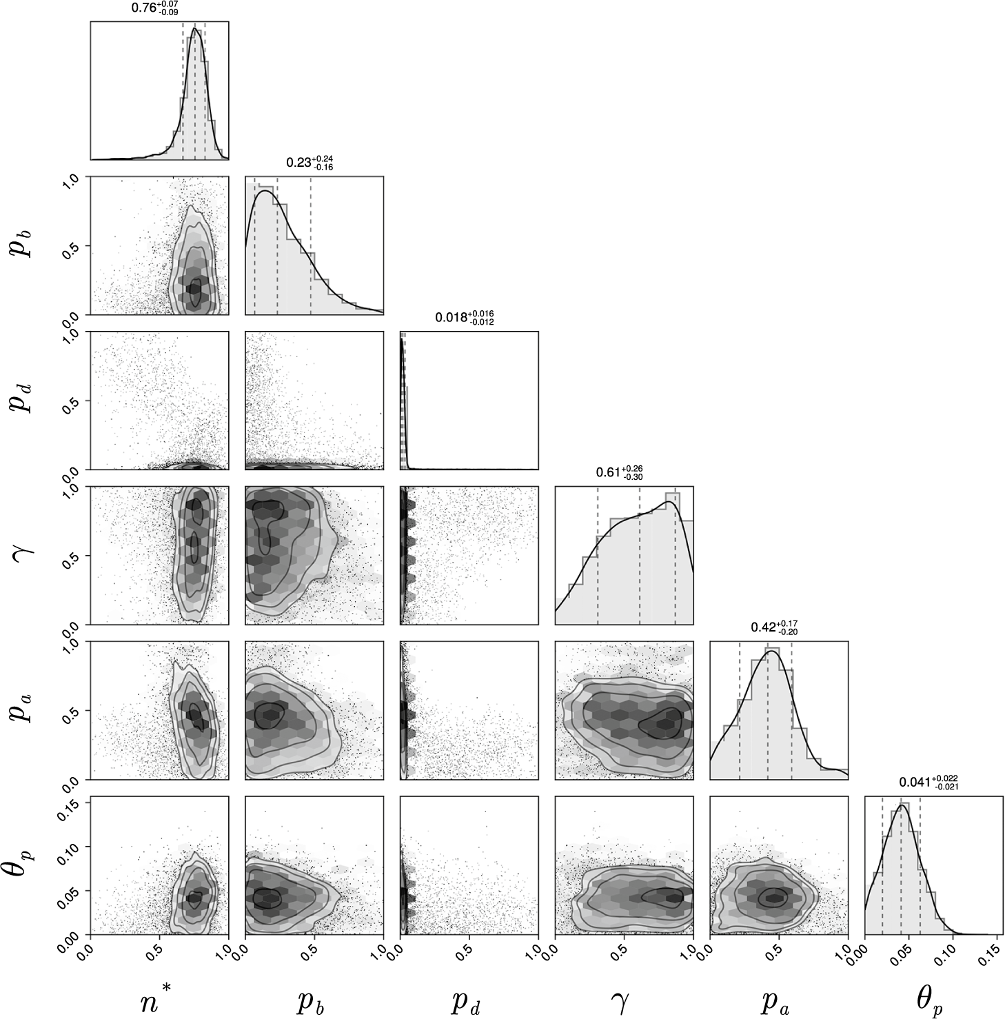
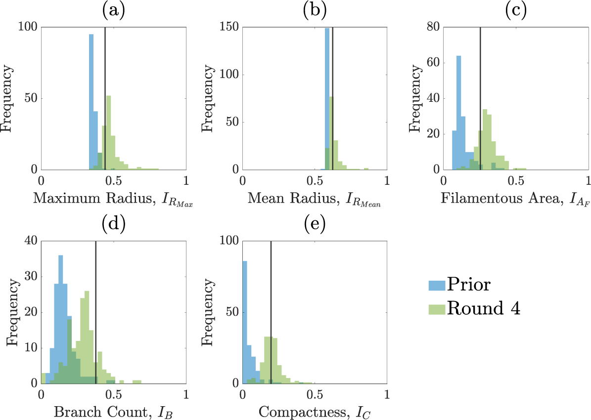
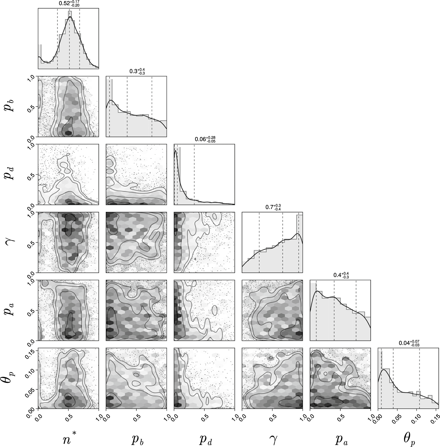
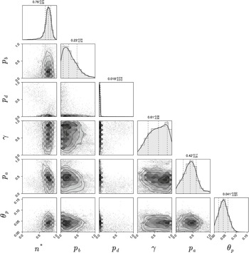
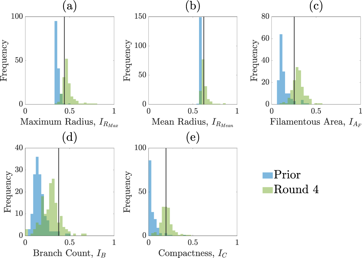
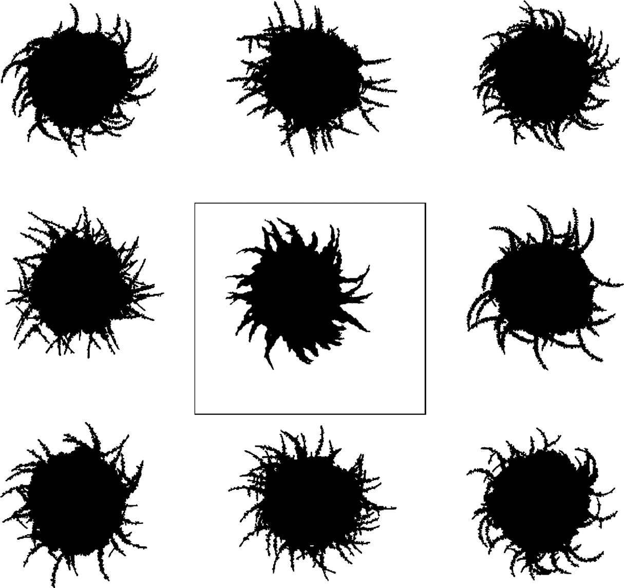
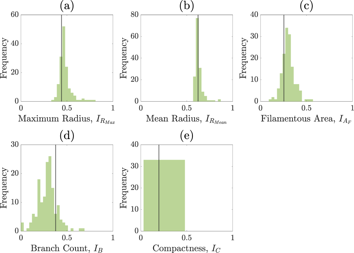
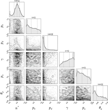
We perform the inference on a single experimental image to avoid issues of inter-experiment variability. A pair plot of the posterior distribution is shown in Figure 7. Figure 8 shows prior and posterior predictive distributions for the five summary statistics, and Figure 9 shows simulations from eight sets of parameters randomly sampled from the posterior. The observed summary statistics are in all cases in the tails of the prior predictive distribution, but the posterior predictive distributions’ modes are mostly centred on them, indicating that the inference algorithm is performing correctly. We also present the posterior from the initial round of training in Figure C.6 (Appendix C) to demonstrate that the posterior from the initial round is much wider and less informative than the posterior after 4 rounds. Figure 9 provides an additional visual demonstration that the inferred parameters are capturing the correct morphology, with patterns resembling the experimental image.
Pair plot of posterior distributions after three iterations of the sequential neural likelihood estimation. All priors were uniform over the axes ranges shown in the figure.
Normalized summary statistics generated from sampling from either the prior or from the posterior distribution after four rounds of SNLE. The vertical line represents the summary statistic from the experimental colony shown in Figure 6. Blue histograms are of the summary statistics for simulations sampled from the prior and the green histograms are for simulations sampled from the posterior distribution after round 4 of the SNLE. (a) Maximum radius. (b) Mean radius. (c) Filamentous area. (d) Branch count. (e) Compactness.
A binary image of an experimentally produced colony of M. magnusii grown on YNB containing  ammonium sulfate (centre panel), flanked by eight simulations drawn from the posterior from Figure 7.

The data are informative for all parameters except $\gamma $
. The parameters
$\gamma $
. The parameters $n^*$
and
$n^*$
and $p_d$
are strongly identified, whereas the marginal posteriors for
$p_d$
are strongly identified, whereas the marginal posteriors for $p_b,\, p_a$
and
$p_b,\, p_a$
and $\theta _p$
are broad, meaning that these parameters are only weakly identified. As expected, the threshold for initiation of spiral filamentation,
$\theta _p$
are broad, meaning that these parameters are only weakly identified. As expected, the threshold for initiation of spiral filamentation, $n^*$
, is inferred well with a tight marginal posterior with mode of 0.76. This parameter is essential in controlling when filamentation begins, which is important in determining the overall morphology and size of the colony. The parameter
$n^*$
, is inferred well with a tight marginal posterior with mode of 0.76. This parameter is essential in controlling when filamentation begins, which is important in determining the overall morphology and size of the colony. The parameter $p_d$
, which is the probability that a filament-forming agent emanates from a regular agent, is strongly inferred to be small. If
$p_d$
, which is the probability that a filament-forming agent emanates from a regular agent, is strongly inferred to be small. If $p_d$
is small, we expect fewer longer spiralling filaments, whereas a large
$p_d$
is small, we expect fewer longer spiralling filaments, whereas a large $p_d$
would produce more, shorter spiralling filaments. From the experimental images, we anticipate smaller values of
$p_d$
would produce more, shorter spiralling filaments. From the experimental images, we anticipate smaller values of $p_d$
because filaments are distinct and long, and this is confirmed by the marginal posterior that puts almost all mass on values
$p_d$
because filaments are distinct and long, and this is confirmed by the marginal posterior that puts almost all mass on values $p_d<0.1$
.
$p_d<0.1$
.
Another crucial parameter in our model is the angle between successive segments, $\theta _p$
, as this determines the amount of spiralling. This parameter could be identified and its mode is
$\theta _p$
, as this determines the amount of spiralling. This parameter could be identified and its mode is $0.041$
radians (2.3 degrees). This result provides an estimate of the angle, which has not previously been quantified for M. magnusii. Although the angle is small, it still gives rise to observable colony-scale spiral patterns, as Figure 9 shows. Since
$0.041$
radians (2.3 degrees). This result provides an estimate of the angle, which has not previously been quantified for M. magnusii. Although the angle is small, it still gives rise to observable colony-scale spiral patterns, as Figure 9 shows. Since $\theta _p$
is constant in the model, within each simulated colony, the spirals tend to have similar arc radii, with some variation that reflects the variation in the experimental image. The model can also reproduce characteristic microscopic patterns within the filamentous regions themselves (see Appendix A for further details).
$\theta _p$
is constant in the model, within each simulated colony, the spirals tend to have similar arc radii, with some variation that reflects the variation in the experimental image. The model can also reproduce characteristic microscopic patterns within the filamentous regions themselves (see Appendix A for further details).
The probability $p_a$
governs whether a regular or filament-forming hypha is chosen to produce a new segment. This parameter is weakly identified, suggesting that capturing the initial emergence of filament-forming hyphae and the angle between successive segments are more important for predicting the morphological features captured by the summary statistics. Similarly,
$p_a$
governs whether a regular or filament-forming hypha is chosen to produce a new segment. This parameter is weakly identified, suggesting that capturing the initial emergence of filament-forming hyphae and the angle between successive segments are more important for predicting the morphological features captured by the summary statistics. Similarly, $p_b$
is weakly identified. Changes to this parameter influence the thickness of the filaments by allowing regular hyphae to form alongside filament-forming ones. Since our summary statistics do not contain a metric that explicitly quantifies the width or curvature of filaments, this parameter cannot be well inferred. The data are uninformative for the parameter
$p_b$
is weakly identified. Changes to this parameter influence the thickness of the filaments by allowing regular hyphae to form alongside filament-forming ones. Since our summary statistics do not contain a metric that explicitly quantifies the width or curvature of filaments, this parameter cannot be well inferred. The data are uninformative for the parameter $\gamma .$
This parameter, which controls forking from filament-forming segments, was important for the pseudohyphal S. cerevisiae yeast growth of Li et al. [Reference Li, Green, Tronnolone, Tam, Black, Gardner, Sundstrom, Jiranek and Binder37], but is poorly identified for these hyphal M. magnusii colonies. These results suggest that the value of
$\gamma .$
This parameter, which controls forking from filament-forming segments, was important for the pseudohyphal S. cerevisiae yeast growth of Li et al. [Reference Li, Green, Tronnolone, Tam, Black, Gardner, Sundstrom, Jiranek and Binder37], but is poorly identified for these hyphal M. magnusii colonies. These results suggest that the value of $\gamma ,$
and hence the forking control process, is less important for determining the M. magnusii morphology.
$\gamma ,$
and hence the forking control process, is less important for determining the M. magnusii morphology.
The statistics for maximum radius, mean radius and compactness are especially well predicted by our posterior predictive simulations (see Figure 8). There is larger variability in the filamentous area and branch count among the simulations, although overall, the simulations still align well with the experiment. Variability in both the filamentous area and branch count is consistent with the finding that parameters affecting filament width are only weakly identified due to the summary statistics not capturing filament width.
5 Other M. magnusii yeast morphologies
In different experimental conditions, M. magnusii colonies form different morphologies. We explore these morphologies through additional simulations of the model. In a nutrient-rich environment, the yeast tends to grow in a rounded hexagonal shape as shown in Figure 10(a), reminiscent of Eden-like growth [Reference Eden24]. Although the round colony does not exhibit irregular filamentation, the almost hexagonal perimeter we see in the simulation mimics the experiment, which could be due to the shape and pattern of growth for regular hyphae. Under other conditions, M. magnusii has also been shown to have straight filaments of varying thicknesses as shown in Figures 10(b) and 10(c). These patterns are more similar to the patterns formed by hyphal colonies of the important pathogenic yeast C. albicans [Reference Berman and Sudbery8, Reference Cleary, Mulabagal, Reinhard, Yadev, Murdoch, Thornhill, Lazzell, Monteagudo, Thomas and Saville19, Reference Mohammadi, Leduc, Charette, Barbeau and Vincent47]. With specifically chosen parameter values, we can also capture these patterns in model simulations, as presented in Figures 10(d)–10(f).
Other M. magnusii yeast morphologies under varying environmental conditions. (a) Experimental colony grown on CDS with low yeast density. (b) Experimental colony grown on CDS at high yeast density. (c) Experimental colony grown on YNB at high yeast density. (d) Simulation with $n_{\text {max}} = 10\,000$
agents, and parameters
$n_{\text {max}} = 10\,000$
agents, and parameters $n^* = 1$
,
$n^* = 1$
, $p_a=0.25$
,
$p_a=0.25$
, $p_b=0.3$
,
$p_b=0.3$
, $p_d=0.1$
,
$p_d=0.1$
, $\gamma = 0.05$
and
$\gamma = 0.05$
and $\theta _p=0.05$
. (e) Simulation with
$\theta _p=0.05$
. (e) Simulation with $n_{\text {max}} = 10\,000$
agents, and
$n_{\text {max}} = 10\,000$
agents, and $n^* = 0.6$
,
$n^* = 0.6$
, $p_a=0.25$
,
$p_a=0.25$
, $p_b=0.3$
,
$p_b=0.3$
, $p_d=0.1$
,
$p_d=0.1$
, $\gamma = 0.05$
and
$\gamma = 0.05$
and $\theta _p=0.05$
. (f) Simulation with
$\theta _p=0.05$
. (f) Simulation with $n_{\text {max}} = 10\,000$
agents, and
$n_{\text {max}} = 10\,000$
agents, and $n^* = 0.5$
,
$n^* = 0.5$
, $p_a=0.1$
,
$p_a=0.1$
, $p_b=0.02$
,
$p_b=0.02$
, $p_d = 1$
,
$p_d = 1$
, $\gamma = 0.90$
and
$\gamma = 0.90$
and $\theta _p=0.05$
.
$\theta _p=0.05$
.
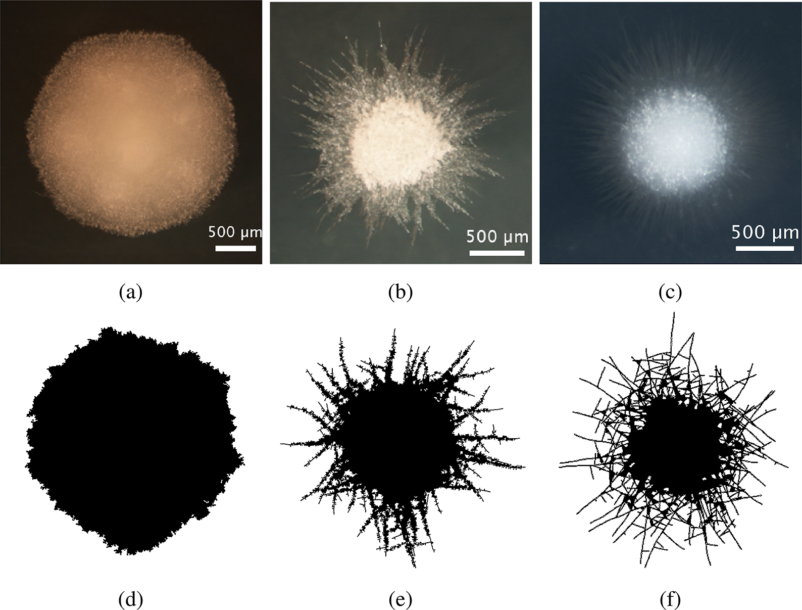
The ability to capture multiple experimentally feasible M. magnusii morphologies suggests that our off-lattice model is consistent with the biology of hyphal growth. Furthermore, differences in parameter values across the three simulations in Figure 10 may indicate how the environment influences M. magnusii growth. In the hexagonal colony of Figures 10(a) and 10(d), the threshold for filament-forming hyphae is set to $n^* = 1,$
whereas this parameter is
$n^* = 1,$
whereas this parameter is $n^* = 0.6$
and
$n^* = 0.6$
and $n^* = 0.5$
for the other colonies. The experimental colony in Figure 10(a) was grown on CDS media with low density of colonies within the culture well, whereas the colonies in Figures 10(b) and 10(c) were grown under conditions of high colony density. The differences in
$n^* = 0.5$
for the other colonies. The experimental colony in Figure 10(a) was grown on CDS media with low density of colonies within the culture well, whereas the colonies in Figures 10(b) and 10(c) were grown under conditions of high colony density. The differences in $n^*$
indicate that M. magnusii does not experience low-nutrient stress in the low colony density case, but does in high-density environments, where more colonies compete for the same nutrients. These results are consistent with the hypothesis that the transition between regular and filament-forming hyphae is mediated by nutrient availability. In contrast, the proliferation angle
$n^*$
indicate that M. magnusii does not experience low-nutrient stress in the low colony density case, but does in high-density environments, where more colonies compete for the same nutrients. These results are consistent with the hypothesis that the transition between regular and filament-forming hyphae is mediated by nutrient availability. In contrast, the proliferation angle $\theta _p$
is held constant across all three simulations in Figure 10(d–f). Since
$\theta _p$
is held constant across all three simulations in Figure 10(d–f). Since $\theta _p$
was identifiable in the parameter inference, this angle could be an intrinsic feature of M. magnusii growth regardless of environment. Finally, although
$\theta _p$
was identifiable in the parameter inference, this angle could be an intrinsic feature of M. magnusii growth regardless of environment. Finally, although $p_b$
and
$p_b$
and $\gamma $
were difficult to identify, comparing the simulations in Figures 10(e) and 10(f) reveals their effect. The simulation with larger
$\gamma $
were difficult to identify, comparing the simulations in Figures 10(e) and 10(f) reveals their effect. The simulation with larger $p_b,$
smaller
$p_b,$
smaller $\gamma $
and smaller
$\gamma $
and smaller $p_d$
favours thicker hyphal filaments (Figure 10(e)), because regular hyphal segments are more likely to occur within filaments. Conversely, the simulation with smaller
$p_d$
favours thicker hyphal filaments (Figure 10(e)), because regular hyphal segments are more likely to occur within filaments. Conversely, the simulation with smaller $p_b,$
larger
$p_b,$
larger $\gamma $
and larger
$\gamma $
and larger $p_d$
is more likely to produce filaments, but less likely to contain regular hyphae within filaments, creating the thinner filaments seen in Figure 10(f).
$p_d$
is more likely to produce filaments, but less likely to contain regular hyphae within filaments, creating the thinner filaments seen in Figure 10(f).
6 Discussion and conclusion
In this paper, we have presented an off-lattice agent-based modelling and parameter inference procedure that yields biological insight into small yeast colonies formed in harsh environments. We applied this procedure to a new strain of M. magnusii recently bioprospected from a Tasmanian cider gum tree. Since this strain produced a spiral-like morphology, we adapted our agent-based model to incorporate hyphal segments and extension at a constant angle between successive segments. We used image processing and spatial statistics to compare the shape of simulated colonies with the experiment. Using Bayesian inference, we estimated the mean angle between segments to be ${2.3}^{\circ } [{1.1}^{\circ }, {3.6}^{\circ }]$
(95% credible interval), a result that has not previously been quantified. One potential limitation of our method is that the termination criterion was tuned to match the observed area, while size-based summary statistics were also used, which might produce overconfident posteriors. However, colonies simulated using the inferred parameters closely resembled those from the experiment. We also extended this result further to obtain simulations of other experimentally realized shapes with different parameters. We also provide open-source code for the agent-based models and parameter estimation techniques on GitHubFootnote 1 .
${2.3}^{\circ } [{1.1}^{\circ }, {3.6}^{\circ }]$
(95% credible interval), a result that has not previously been quantified. One potential limitation of our method is that the termination criterion was tuned to match the observed area, while size-based summary statistics were also used, which might produce overconfident posteriors. However, colonies simulated using the inferred parameters closely resembled those from the experiment. We also extended this result further to obtain simulations of other experimentally realized shapes with different parameters. We also provide open-source code for the agent-based models and parameter estimation techniques on GitHubFootnote 1 .
Our work provides a framework for understanding the colony patterns formed by new yeast strains uncovered by bioprospecting. Adapting the agent-based model to meet the biological assumptions and performing parameter inference will allow researchers to gain insight into the key cell-level mechanisms underpinning the patterns. Improvements for future work could also include a summary statistic to capture the thickness of branches, which might make the parameter $p_b$
more identifiable. Additionally, this paper has reviewed several forms of surface growth in yeast colonies. However, in some experiments, yeast cells grow on the surface and also penetrate into the agar medium [Reference Cullen and Sprague20]. This invasive growth is of great interest to biologists due to its importance for pathogenic infections. In future work, we intend to extend the modelling and parameter inference methods to three-dimensions to investigate this invasive growth phenomenon. From the biological perspective, the environmental and genetic drivers of spiralling in M. magnusii remain to be fully understood. In the mould fungus Neurospora crassa, the gene coil-1 promotes spiralling or coiling [Reference Beever7], and yeast morphologies broadly depend on genetic and environmental factors [Reference Granek and Magwene31]. Future experimental work could involve disrupting specific genes or growing M. magnusii in varying conditions to assess how these factors affect spiral formation.
$p_b$
more identifiable. Additionally, this paper has reviewed several forms of surface growth in yeast colonies. However, in some experiments, yeast cells grow on the surface and also penetrate into the agar medium [Reference Cullen and Sprague20]. This invasive growth is of great interest to biologists due to its importance for pathogenic infections. In future work, we intend to extend the modelling and parameter inference methods to three-dimensions to investigate this invasive growth phenomenon. From the biological perspective, the environmental and genetic drivers of spiralling in M. magnusii remain to be fully understood. In the mould fungus Neurospora crassa, the gene coil-1 promotes spiralling or coiling [Reference Beever7], and yeast morphologies broadly depend on genetic and environmental factors [Reference Granek and Magwene31]. Future experimental work could involve disrupting specific genes or growing M. magnusii in varying conditions to assess how these factors affect spiral formation.
A Appendix: Enlarged simulation result
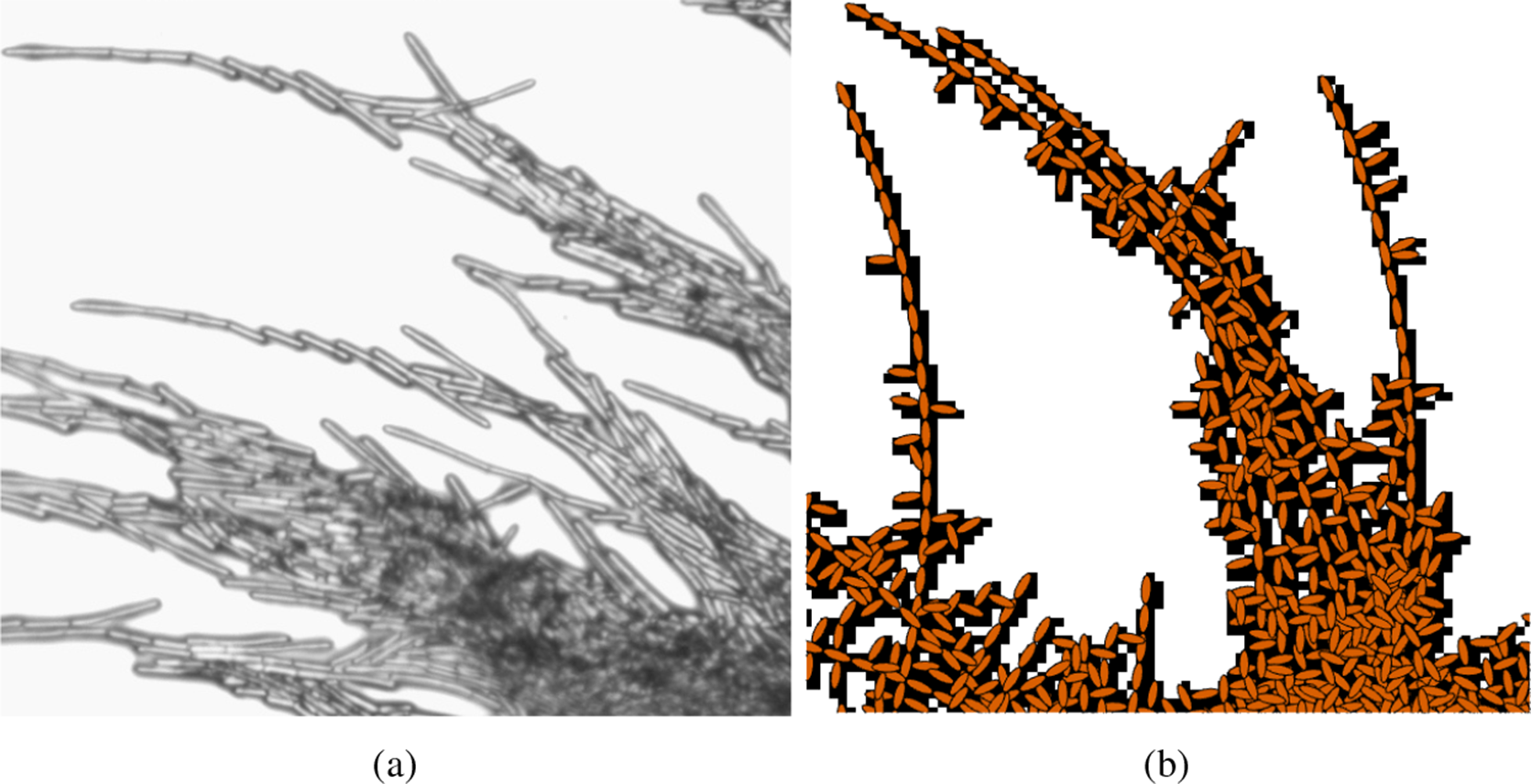
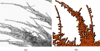
Figure A.1 compares the microscopic detail in the filamentous region between an experiment and a simulation of M. magnusii. These enlarged images indicate that the agent-based model can successfully represent the spiral filament-forming process.
Comparison of an experiment and simulation (not to scale). (a) Enlarged view of the filamentous region of a M. magnusii colony from one of our experiments. (b) A typical agent-based simulation, enlarged in near a hyphal filament. Brown ellipses indicate the locations of hyphal segments and the black overlay indicates the area considered to be occupied by the simulated colony after binarization.
B Appendix: Multiple agent sizes
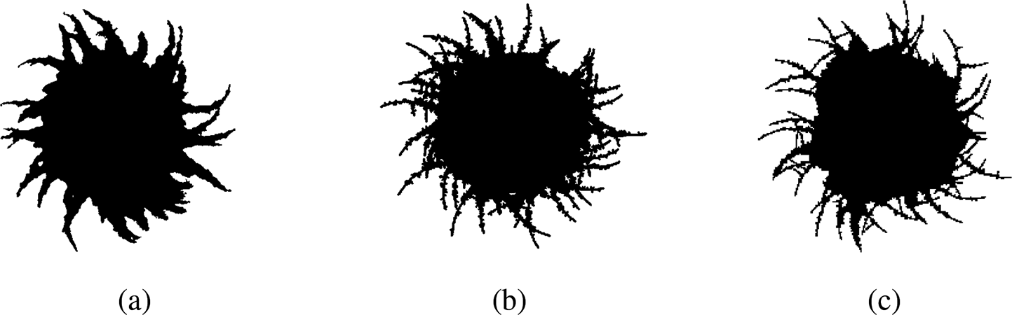
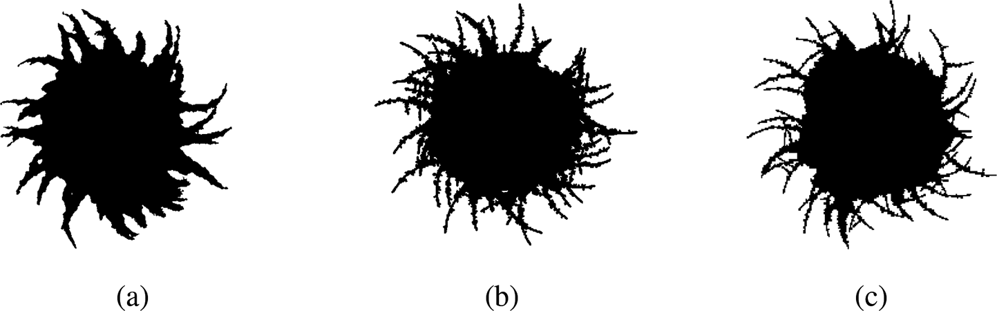
We also investigate the effect of agent shape on the spiral yeast morphology. To demonstrate that the colony morphology is robust to changes in agent shape, we simulate colonies where the regular hyphal segments and filamentous hyphal segments have different geometry (Figure B.1). We use the same parameter values as in Figure 9, varying only the agent shape. There is minimal difference between the three colonies, suggesting that other parameters such as $\theta _p$
drive the spiral colony morphology in M. magnusii.
$\theta _p$
drive the spiral colony morphology in M. magnusii.
(a) Experiment of M. magnusii grown on YNB medium. (b) Spiral yeast simulation with parameters $n^*=0.76$
,
$n^*=0.76$
, $p_a=0.42$
,
$p_a=0.42$
, $p_b=0.23$
,
$p_b=0.23$
, $p_d=0.02$
,
$p_d=0.02$
, $\gamma = 0.77$
and
$\gamma = 0.77$
and $\theta _p=0.04$
, drawn from the posterior distribution. All agents have the same size, with aspect ratio 0.33. (c) Spiral yeast simulation with the same parameters as panel (b), but two possible agent sizes, with aspect ratios 0.75 (regular) and 0.33 (filament-forming). Each agent has the same area.
$\theta _p=0.04$
, drawn from the posterior distribution. All agents have the same size, with aspect ratio 0.33. (c) Spiral yeast simulation with the same parameters as panel (b), but two possible agent sizes, with aspect ratios 0.75 (regular) and 0.33 (filament-forming). Each agent has the same area.
C Appendix: Additional parameter inference results
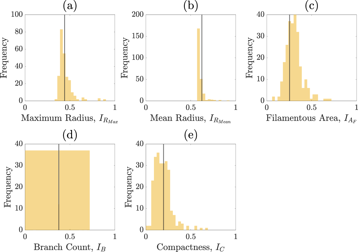
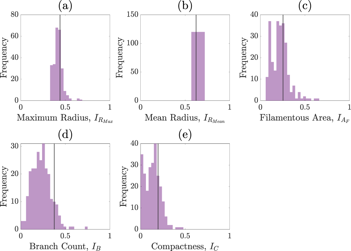
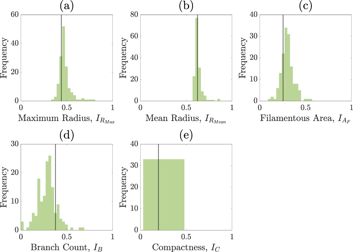
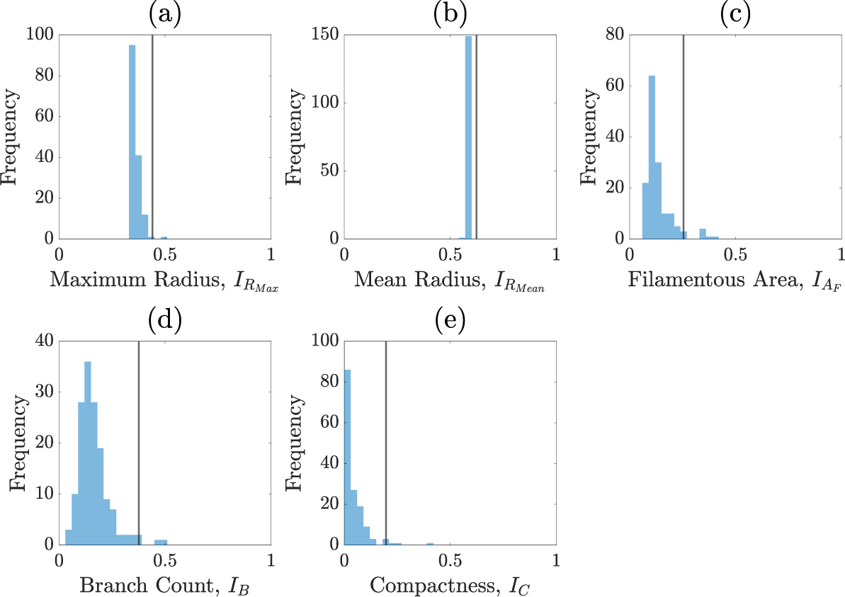
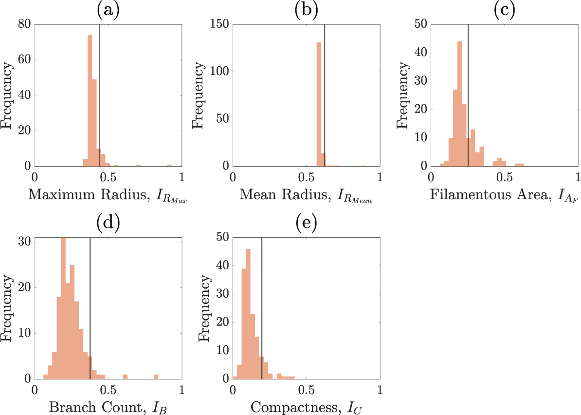
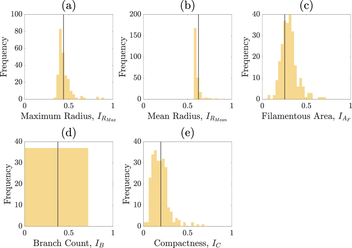
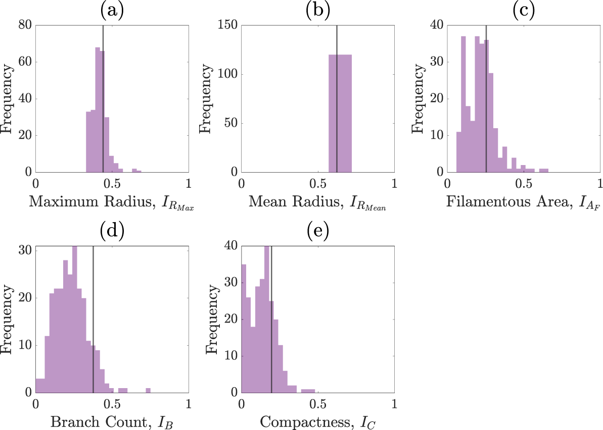
Figures C.1–C.5 show the summary statistics obtained after each round of sequential neural likelihood applied to the experimental image.
Summary statistics of the priors.
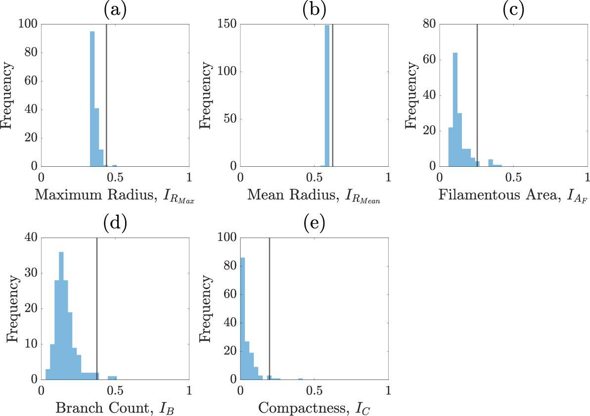
Summary statistics of round one.
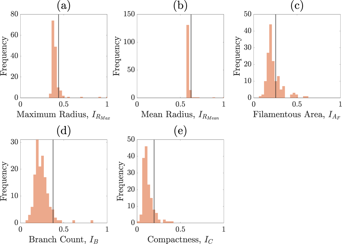
Summary statistics of round two.
Summary statistics of round three.
Summary statistics of round four.
Pair plot of posterior distributions after the initial round of the neural likelihood estimation.
D Appendix: SNLE details
We use a Gaussian mixture density network (MDN) as our surrogate likelihood model [Reference Bishop10], which is implemented using the MixtureDensityNetworks.jl package in Julia. The parameters $\boldsymbol {\theta } = (n^*, p_b, p_d, \gamma , p_a, \theta _p)$
are constrained to
$\boldsymbol {\theta } = (n^*, p_b, p_d, \gamma , p_a, \theta _p)$
are constrained to $[1,0]^5 \times [0, \pi /20]$
; hence, we apply a logit transform and fit the surrogate likelihood model in an unconstrained space. Posterior sampling was also carried out in this space and then the resulting samples were transformed back to constrained space for visualization and analysis.
$[1,0]^5 \times [0, \pi /20]$
; hence, we apply a logit transform and fit the surrogate likelihood model in an unconstrained space. Posterior sampling was also carried out in this space and then the resulting samples were transformed back to constrained space for visualization and analysis.
The architecture of the MDN was chosen to be the same as that of Li et al. [Reference Li, Tam, Gardner, Sundstrom, Jiranek, Green, Binder and Black39], which worked well for a similar model and posterior geometry. The MDN had two hidden layers of width 64 and six mixtures. The MDN was trained using the Adam optimizer with a learning rate of $1\times 10^{-3}$
, a batch size of 16 and for 600 epochs. Convergence was assessed by examining the loss over the number of epochs.
$1\times 10^{-3}$
, a batch size of 16 and for 600 epochs. Convergence was assessed by examining the loss over the number of epochs.
For each round of training a dataset of 1000 simulations from the ABM was generated, which is equivalent to approximately 24 hours of high-computing time. Then, posterior sampling was performed using a basic Metropolis–Hastings algorithm. This used a basic Gaussian random walk proposal with standard deviation 1. We generated 200 000 MCMC samples to ensure adequate convergence of the posterior distribution, discarding the first 10,000 samples as burn-in and applying a thinning factor of 10 to reduce autocorrelation, resulting in an effective sample size exceeding $550$
for each parameter. Owing to the simple geometry of the posterior in each round, the Markov chain mixed rapidly, requiring minimal manual tuning. It was found that four rounds of training were sufficient for convergence of the approximate posterior, which was assessed visually by changes in the distribution over rounds as well as the distributions of the summary statistics.
$550$
for each parameter. Owing to the simple geometry of the posterior in each round, the Markov chain mixed rapidly, requiring minimal manual tuning. It was found that four rounds of training were sufficient for convergence of the approximate posterior, which was assessed visually by changes in the distribution over rounds as well as the distributions of the summary statistics.
Acknowledgments
K.L. acknowledges funding from the Australian Government through a Research Training Program (RTP) Scholarship. V.J., J.E.F.Gr., B.J.B. and A.K.Y.T. acknowledge funding from the Australian Research Council (Grant numbers DP230100406 and DE240100097). The authors acknowledge supercomputing resources from The University of Adelaide’s maths1 High Performance Computing (HPC) service.








 Open access

