

1. INTRODUCTION
Ice shelves are floating ice masses connected to and nourished by land-based ice. They are thought to exert an important control on the dynamics of the grounded ice-sheet sectors (Rignot and others, Reference Rignot2004; Dupont and Alley, Reference Dupont and Alley2005; Rott and others, Reference Rott, Müller, Nagler and Floricioiu2011; Gudmundsson, Reference Gudmundsson2013), buttressing and buffering the ice flux where it reaches the ocean. Thus, ice shelf thinning and removal holds an indirect, albeit significant potential for a contribution to sea-level variations. Recent studies have shown that changes in the ocean thermal state play a critical role in ice-shelf thinning and a subsequent loss of buttressing (e.g., Pritchard and others, Reference Pritchard2012). Present-day observations suggest that over a half of the Antarctic mass loss is due to sub-shelf basal melting (Depoorter and others, Reference Depoorter2013; Rignot and others, Reference Rignot, Jacobs, Mouginot and Scheuchl2013), with melting rates ranging from a few centimeters to tens of meters per year, and values near grounding lines exceeding area-averaged rates by one to two orders of magnitude (Rignot and others, Reference Rignot and Jacobs2002). Since basal melt rates are likely to increase in the future due to increasing ocean temperatures (e.g. Gillett and others, Reference Gillett, Arora, Zickfeld, Marshall and Merryfield2011; Yin and others, Reference Yin2011; Hellmer and others, Reference Hellmer, Kauker, Timmermann, Determann and Rae2012), a better understanding of their magnitudes and spatial distribution is a crucial requirement for reliable projections of the ice-sheet evolution and sea-level rise (Joughin and others, Reference Joughin, Alley and Holland2012).
Net melt rates under ice shelves have been previously estimated using different techniques based on surrounding oceanographic data (Gammelsrod and others, Reference Gammelsrod, Johannessen, Muench and Overland1994; Foldvik and others, Reference Foldvik, Gammelsrod, Nygaard and Osterhus2001; Jenkins and Jacobs, Reference Jenkins and Jacobs2008; Jacobs and others, Reference Jacobs, Jenkins, Giulivi and Dutrieux2011), local glaciological observations (Doake, Reference Doake1984; Jacobs and others, Reference Jacobs, Hellmer, Doake, Jenkins and Frolich1992; Rignot and others, Reference Rignot and Jacobs2002; Joughin and Padman, Reference Joughin and Padman2003; Wen and others, Reference Wen2010) and satellite data (Depoorter and others, Reference Depoorter2013; Rignot and others, Reference Rignot, Jacobs, Mouginot and Scheuchl2013). Numerical ocean modelling has provided high-resolution reconstructions of basal melt rates under a number of individual ice shelves (Gerdes and others, Reference Gerdes, Determann and Grosfeld1999; Jenkins and Holland, Reference Jenkins and Holland2002; Holland and others, Reference Holland, Corr, Vaughan, Jenkins and Skvarca2009, Reference Holland, Jenkins and Holland2010; Hellmer and others, Reference Hellmer, Kauker, Timmermann, Determann and Rae2012; Padman and others, Reference Padman2012; Schodlok and others, Reference Schodlok, Menemenlis, Rignot and Studinger2012) and total ice-shelf meltwater production estimates from circumpolar simulations (Hellmer, Reference Hellmer2004; Timmermann and others, Reference Timmermann, Wang and Hellmer2012). These studies have presented total ice-shelf basal mass balance (BMB) estimates ranging from ~ −500 to ~ −1700 Gt a−1. Recent estimates based on satellite data (Depoorter and others, Reference Depoorter2013; Rignot and others, Reference Rignot, Jacobs, Mouginot and Scheuchl2013) have uncovered the spatial distribution of the melting and freezing zones for the entire Antarctic ice-shelf system. Although the total BMB estimates provided by these particular studies are comparable and within the above-mentioned range, they disagree in the contributions of individual ice-shelf sectors (Depoorter and others, Reference Depoorter2013; Rignot and others, Reference Rignot, Jacobs, Mouginot and Scheuchl2013).
Ice flow models require an accurate quantification of the ice-shelf BMB to reproduce the dynamics of ice when it is in contact with the ocean. Due to scarcity of whole-Antarctic BMB estimates in the past and high computational costs of coupled regional ocean-ice-sheet modelling experiments, stand-alone continental-scale ice models have so far mostly relied on simplified parameterisations to account for ice/ocean interactions. These approaches range from a prescription of a single-value (spatially uniform) basal melting rates over the entire domain (e.g. Bindschadler and others, Reference Bindschadler2013) to simplified parameterisations using homogeneous or modelled (extrapolated) ocean temperatures (e.g. Beckmann and Goosse, Reference Beckmann and Goosse2003; Holland and others, Reference Holland, Jenkins and Holland2008), which are kept constant in space and time (e.g. Martin and others, Reference Martin2011; de Boer and others, Reference de Boer2015). These parameterisations are commonly calibrated against the observed ice volumes and extents, and the resulting melting rates are not necessarily consistent with the oceanographic and glaciological BMB estimates. Furthermore, these parameterisations usually disregard sub-shelf freezing processes that have been shown by observational studies to occur under vast portions of the Antarctic ice shelves.
Here, we build upon the concepts used to interpret observations (Depoorter and others, Reference Depoorter2013; Rignot and others, Reference Rignot, Jacobs, Mouginot and Scheuchl2013) and implement a method combining stand-alone ice-sheet-shelf simulations and topographic data (Bernales and others, Reference Bernales, Rogozhina, Greve and Thomas2017) to quantify sub-shelf melting and freezing rates. With this novel approach, we derive total, sector- and ice shelf-specific BMB values that can be directly compared with previous glaciological and oceanographic estimates. Furthermore, the use of a numerical model allows us to explore the sensitivity of the results to changes in the model grid resolution, and uncertainties in the input data-sets and model parameters.
2. METHODS
2.1. Ice-sheet-shelf model
We use the ice-sheet-shelf model SICOPOLIS (SImulation COde for POLythermal ice sheets) version 3.2, revision 619 (Greve and Blatter, Reference Greve and Blatter2009; Sato and Greve, Reference Sato and Greve2012). The model set-up closely follows that of Bernales and others (Reference Bernales, Rogozhina, Greve and Thomas2017). The experiments described in this study use a one-layer enthalpy scheme recently implemented in the model (Greve and Blatter, Reference Greve and Blatter2016). Additional modifications to the model specifically for this study are presented below.
At its core, the model solves for the ice velocity using finite-difference implementations of the Shallow Ice and Shallow Shelf Approximations (SIA and SSA, respectively; e.g. Hutter, Reference Hutter1983; Morland, Reference Morland1987). The SSA is used to compute ice velocities of ice shelves, which experience almost no friction at their interface with sea water, whereas the SIA is used across the grounded ice-sheet sectors, where the mechanical properties of the bedrock and crustal heat flow create a variety of friction conditions, ranging from nearly immobile ice masses frozen to bed to fast flowing ice streams sliding over water-saturated sediments. Since basal sliding is not accounted for in the SIA, ice flow models have traditionally implemented various empirical sliding laws as an additional boundary condition. Bueler and Brown (Reference Bueler and Brown2009) proposed to use a modified SSA including basal drag (also known as the Shelfy Stream Approximation, SStA) as a sliding law, showing that this heuristic, ‘hybrid’ combination of the SIA and the SStA is able to reproduce most ice flow regimes. Bernales and others (Reference Bernales, Rogozhina, Greve and Thomas2017) compared different implementations of this idea, and in this study we are using a modification of the approach proposed by Winkelmann and others (Reference Winkelmann2011), as follows: first, the SIA velocities are computed while setting basal velocities to zero. Then, the SStA velocities are computed using a Weertman-type sliding law (see Bernales and others, Reference Bernales, Rogozhina, Greve and Thomas2017, Eqns (2)–(6)) with a basal drag coefficient that has been calibrated to minimise the difference between the modelled and observed ice-thickness data (Pollard and DeConto, Reference Pollard and DeConto2012; Bernales and others, Reference Bernales, Rogozhina, Greve and Thomas2017). Finally, both solutions are combined over the entire ice sheet using
 $${\bf U} = (1 - w) \cdot {\bf u}_{{\bf sia}} + {\bf u}_{{\bf ssta}},$$
where  ${\bf u}_{{\rm sia}}$ and ${\bf u}_{{\rm ssta}}$ are the SIA and SStA horizontal velocities, respectively, and w is a weight computed following Bueler and Brown (Reference Bueler and Brown2009):
 $$w( \vert {\bf u}_{{\rm ssta}} \vert ) = \displaystyle{2 \over \pi} {\rm arctan}\left( {\displaystyle{{ \vert {\bf u}_{{\rm ssta}} \vert ^2} \over {u_{{\rm ref}}^2}}} \right),$$
where u ref is a reference velocity, set to 30 m a−1, following Bernales and others (Reference Bernales, Rogozhina, Greve and Thomas2017). This particular scheme decreases the contribution of the SIA velocities in areas where high SStA velocities are detected. Such fast flowing areas are mostly located near ice-sheet margins, where ice streams operate and the assumptions behind the SIA are no longer valid. The hybrid scheme presented in this study reduces instabilities in these regions caused by artificially high SIA velocities, the absence of which is assumed but not assured by Winkelmann and others (Reference Winkelmann2011). The resulting ice velocity is used to solve the evolution equations of the ice thickness and temperature (Greve and Blatter, Reference Greve and Blatter2009), providing the main components for the steady-state experiments presented in this study.
2.2. Input data
The observed ice-sheet geometry is derived from the BEDMAP2 dataset (Fretwell and others, Reference Fretwell2013), including bedrock elevation, ice-surface topography, and ice sheet and shelf thickness. The original 1 km-resolution data are regridded to a horizontal resolution of 10 km, currently representing one of the highest resolutions computationally viable for long-term (hundreds of thousands of years), continental-scale forward ice-sheet modelling. BEDMAP2 is a compilation of 24.8 million ice thickness data points obtained from a variety of sources including airborne and over-snow radar surveys, satellite altimetry, seismic sounding data and satellite gravimetry (Fretwell and others, Reference Fretwell2013). Complemented by surface elevation data from several DEMs to derive previously unknown bedrock features, this compilation allows for a detailed modelling of the Antarctic ice sheet-shelf system.
The geothermal heat flux map of Fox Maule and others (Reference Fox Maule, Purucker, Olsen and Mosegaard2005) is prescribed at the base of a modelled lithospheric layer, and the thermal effect at the base of the ice sheet is computed using a temperature equation that balances local temperature changes with advection and heat conduction (Greve and Blatter, Reference Greve and Blatter2009). Atmospheric conditions at the surface of the ice sheet and ice shelves, including near-surface (2 m) air temperatures and precipitation rates, are obtained from the regional climate model RACMO2.3 (henceforth RACMO, van Wessem and others, Reference van Wessem2014), averaged over the period 1979–2010. RACMO is forced at its boundaries by reanalysis data from ERA-Interim over the same period (Dee and others, Reference Dee2011). In the interior of the domain the Antarctic climate conditions are modelled with a horizontal resolution of 27 km and 40 levels in the vertical direction. RACMO contains modules specifically implemented for glaciated regions, including a multilayer snow model, and compares well with in situ observations (van Wessem and others, Reference van Wessem2014).
The precipitation rates and near-surface air temperatures are used to compute the accumulation rates following the relation of Marsiat (Reference Marsiat1994). Temperatures are adjusted to changes in topography through a simple lapse-rate correction of  $0.008{\kern 1pt} {\rm ^\circ} {\rm C}\,{\rm m}^{-1}$. Surface melt is computed using a positive degree-day (PDD; Reeh, Reference Reeh1991; Calov and Greve, Reference Calov and Greve2005) scheme with melt factors β snow = 3 and β ice = 8 mm i.e. day−1 °C−1 for snow and ice, respectively. All forcing datasets have been projected onto the same polar stereographic grid used for the BEDMAP2 data, with a horizontal resolution of 10 km for the main simulation, and 20 and 40 km resolutions for the sensitivity experiments presented in Section 3.2.
2.3. Experimental set-up
The initial bedrock-, sea floor- and basal and surface ice elevations relative to the present-day sea level are defined using the 10 km-spaced topographic data from BEDMAP2 (see Section 2.2). The model domain embraces the entire Antarctic ice sheet-shelf system and the surrounding Southern Ocean, and contains 601 × 601 equidistant gridpoints in the horizontal direction, and 81 gridpoints in the vertical direction (densifying towards the base), used for the computation of the temperature and velocity fields. Below the ice sheet, additional 41 gridpoints form the modelled lithospheric thermal layer. The ice flow enhancement factors for the SIA and SSA are set to the values E SIA = 1 and E SSA = 0.5, respectively. The initial ice temperature for the entire model grid is set to a homogeneous value of  $ - 10{\kern 1pt} {\rm ^\circ} {\rm C}$ (results do not depend on this initial choice). Then, external forcing datasets are prescribed at the boundaries of the system (see Section 2.2): the time-invariant geothermal heat flux data are prescribed as the lower boundary of the thermal bedrock model used to compute the temperatures at the ice-sheet base, whereas the precipitation rates and near-surface temperature are used to compute the surface mass balance and ice-surface temperatures.
From this configuration, the model is run forward in time in four main stages designed to provide a model spin-up and the calibration of two key quantities: the spatial distribution of the basal drag coefficient for the grounded ice sheet, and the basal melting/freezing rates for the floating ice shelves. Initial values for both quantities are 1 m a−1 Pa−1 and 0 m a−1, respectively, corresponding to a rough bedrock that opposes basal sliding and no melt or accretion at the base of ice shelves. Throughout the simulations, the grounding line and ice-shelf fronts are kept at their modern positions in order to ensure a consistent model calibration (Bernales and others, Reference Bernales, Rogozhina, Greve and Thomas2017). In the first stage, the model solves the evolution equations for temperature, velocity and thickness every 5 model-years, during a simulation period of 50 000 years. The distinct feature of this stage is that it scales the evolution of the ice thickness by a factor of 10−3, keeping the ice thickness close to its initial (i.e. observed) value (Bernales and others, Reference Bernales, Rogozhina, Greve and Thomas2017). This allows for an initialisation of the ice-sheet thermodynamics that is not contaminated by artificial changes in the ice geometry. In contrast to a fixed-topography approach (e.g. Pattyn, Reference Pattyn2010; Sato and Greve, Reference Sato and Greve2012), this procedure allows for an evolution of the ice thickness and thus for a continuous calibration of the basal sliding coefficients and basal melt rates during the entire simulation. In addition, it can be combined with a much larger time step (that would otherwise generate numerical instabilities) and ensures that the temperature within the ice can reach an equilibrium with time-invariant boundary conditions at a normal pace, considerably speeding up the simulations.
In the grounded ice sheet, changes in the ice thickness are tracked by a calibration algorithm that adjusts the basal drag coefficient at each grid-point every 50 model-years to locally minimise the difference between the modelled and observed (i.e. initial) ice thickness. This procedure is based on the idea of Pollard and DeConto (Reference Pollard and DeConto2012), which is explored and modified by Bernales and others (Reference Bernales, Rogozhina, Greve and Thomas2017). In the floating ice shelves, a similar algorithm adjusts the magnitude of the basal melting or freezing rates every 20 years, keeping the ice shelves close to their observed thickness, following:
 $${\rm BMR{^\ast}} = {\rm BMR} + F_{{\rm tan}} \cdot {\rm tan}\left( {\displaystyle{{H - H_0} \over {H_{{\rm scl}}}}} \right),$$
where BMR* and BMR are the current and previous basal melting rates (representing freezing if negative), respectively, H and H 0 are the current (modelled) and reference (from BEDMAP2) ice thicknesses, the parameter F tan = 1.725 scales the adjustment and  $H_{{\rm scl}} = 100{\kern 1pt} {\rm m}$ is a scaling factor introduced to prevent overshoots. For the same reason, the argument of the trigonometric function is restricted to a range −1.5 to +1.5 (see Table 2 for experiments with different parameter choices).
The second and third stages use the same set-up (starting from the results of the previous stage), but instead scale the ice-thickness evolution by factors of 10−2 and 10−1, respectively. The final stage involves an unscaled evolution of the ice thickness, solving the thermodynamical model equations every 0.5 years until an equilibrium is reached. These four stages enable a fast, stable convergence towards an equilibrium ice-sheet state. The steady-state experiments presented in this study provide the spatial distribution of basal melting and freezing rates required to keep the Antarctic ice shelves in equilibrium for the simulated dynamical state with a fixed grounding line (see the Supplementary Materials for an analysis of the effects of this constraint). In order to allow for a direct comparison with the observation-based estimates of Rignot and others (Reference Rignot, Jacobs, Mouginot and Scheuchl2013) and Depoorter and others (Reference Depoorter2013), we add (during the post-processing) observation-based ice-shelf thinning rates (Pritchard and others, Reference Pritchard2012) to our steady-state estimates, as a proxy for the ‘non-steady-state’ melt rates. This procedure is qualitatively equivalent to that of Rignot and others (Reference Rignot, Jacobs, Mouginot and Scheuchl2013) and Depoorter and others (Reference Depoorter2013), since these studies use the mass conservation to determine the BMB, while adding the ice-shelf thinning rates to account for a non-equilibrium behaviour. However, the cited studies use 2007/08 ice-surface velocities (Rignot and others, Reference Rignot, Mouginot and Scheuchl2011), which are not necessarily in equilibrium. A comparison between our steady-state ice velocities and the velocities used in Rignot and others (Reference Rignot, Jacobs, Mouginot and Scheuchl2013) and Depoorter and others (Reference Depoorter2013) is presented as part of the results (Section 3.1).
3. RESULTS AND DISCUSSION
3.1. Retrieved basal mass balance of ice shelves
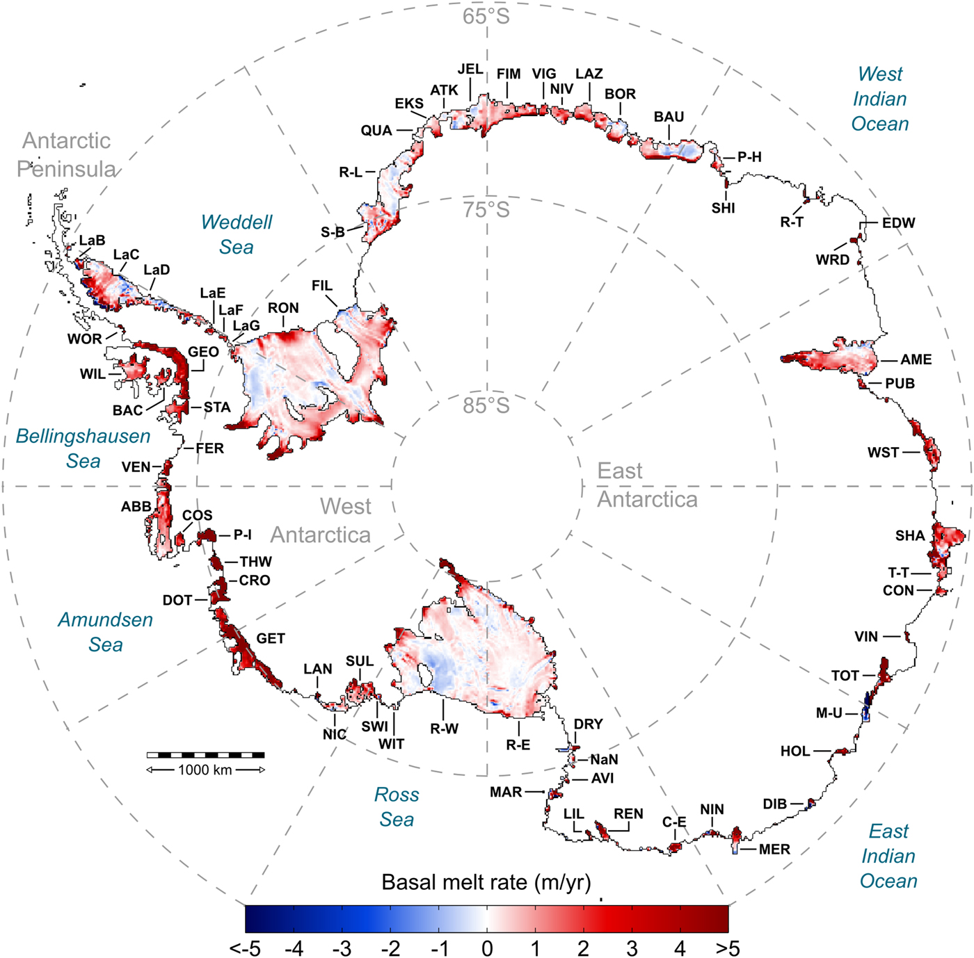
In this section we present the estimated ice-shelf BMB from our simulations of the present-day Antarctic ice sheet, which have been run to an equilibrium with the modern climate conditions. The retrieved distribution of basal melting and freezing rates beneath the Antarctic ice shelves (Fig. 1) is far from being homogeneous, with alternating zones of melting and freezing. The presence of accretion zones is clearly visible under the largest ice shelves (Ronne, Filchner, Ross East and Ross West; see Figure 1 for a location map and Table 1 for abbreviations). Noticeable accretion zones are also present along the coast of East Antarctica, from the Stancomb–Brunt to Prince Harald ice shelves. Overall, the distribution of melting and freezing zones is similar to that of Rignot and others (Reference Rignot, Jacobs, Mouginot and Scheuchl2013), where melting is strongest near grounding lines and ice shelf fronts, while freezing mostly occurs under the central parts of ice shelves (see Supplementary Fig. S2). In addition, we retrieve a predominant melting under the smaller ice shelves whose grounding lines are close to the calving fronts, where the smooth basal topography and small ice-shelf extents prohibit an accretion from ice-shelf-water plumes (Depoorter and others, Reference Depoorter2013). Unexpectedly high rates of basal melting along the East Antarctic coast reported by Rignot and others (Reference Rignot, Jacobs, Mouginot and Scheuchl2013) and Depoorter and others (Reference Depoorter2013) are also reproduced by our model, particularly near grounding lines. In addition, we infer a predominant sub-shelf melting in the West and East Indian Oceans, between the Shirase and Totten ice shelves. As for individual ice shelves, our retrieved patterns closely resemble those from Rignot and others (Reference Rignot, Jacobs, Mouginot and Scheuchl2013) in most areas, with striking similarities in the sub-shelf melting/freezing patterns of the large ice shelves near the ice fronts (see Supplementary Fig. S2).
Predicted basal melting (freezing if negative) rates of Antarctic ice shelves, in metres of ice per year. Modern ice-shelf thinning rates (Pritchard and others, Reference Pritchard2012) are added to account for a non-steady-state behaviour. See Table 1 for details.
Description of individual characteristics of the Antarctic ice shelves, including modelled surface mass balance (SMB), grounding-line flux (GL), ice-front flux (IF), basal mass balance (BMB) and basal melting rate (BMR, with positive values representing melting).

BMB and BMR values include equilibrium (left) and non-steady-state (right) values. BMR values are in w.e., computed using a reference ice density of 910 kg m−3. Text in bold indicates total values for the three major ice sheet sectors and the entire Antarctic ice sheet-shelf system. All values are corrected for area distortions caused by the polar stereographic projection following Snyder (Reference Snyder1987).
Our estimate of the total ice-shelf steady-state BMB is − 1648.7 Gt a−1, which increases to − 1917 Gt a−1 when the observational ice-shelf thinning rates of Pritchard and others (Reference Pritchard2012) are taken into account. The latter value is larger than the estimates of Rignot and others (Reference Rignot, Jacobs, Mouginot and Scheuchl2013) (− 1500 ± 237 Gt a−1) and Depoorter and others (Reference Depoorter2013) (− 1454 ± 174 Gt a−1). The degree of agreement, however, varies for different Antarctic sectors. Our estimates in both the Antarctic Peninsula and West Antarctica are relatively closer to the observation-based studies than in East Antarctica, where our values are considerably higher. This difference reflects generally higher rates of basal melting for many ice shelves, especially near grounding lines required by the model to replicate the observed ice-shelf thickness. These are the areas where the model calibration of the ice-shelf BMB compensates for any excess of influx – relative to an equilibrium – from the grounded ice sheet. We partly attribute our higher estimates to a combination of the following effects:
1. Compared with Rignot and others (Reference Rignot, Jacobs, Mouginot and Scheuchl2013) and Depoorter and others (Reference Depoorter2013), our numerical simulations of the Antarctic ice sheet-shelf system make use of the near-surface temperature and precipitation rate model output from a more recent version of the regional atmospheric model RACMO (van Wessem and others, Reference van Wessem2014). The two versions (RACMO2.3 here and RACMO2.1 in the cited studies) differ in their representation of the atmospheric conditions over East Antarctica, with RACMO2.3 generating considerably wetter conditions dominated by higher snowfall rates (van Wessem and others, Reference van Wessem2014) and therefore a higher ice flux of 1061.7 Gt a−1 into the ice shelves, compared with 782 ± 80 Gt a−1 used by Rignot and others (Reference Rignot, Jacobs, Mouginot and Scheuchl2013).
2. Our calibration of basal melt rates requires a steady influx of ice mass from the grounded glaciers, which is achieved through the calibration of the ice-sheet model using an assumption of an equilibrium with the present-day climate conditions, as described in Section 2. An inclusion of the observed ice-sheet elevation changes during the calibration of continental-scale forward models is, at present, a very challenging task, due to orders-of-magnitude differences between the length of the observational record and the timescales over which these models operate. Thus, recent observations of the ice sheet thickening in East Antarctica (e.g. Davis and others, Reference Davis, Li, McConnell, Frey and Hanna2005; Pritchard and others, Reference Pritchard2012; Shepherd and others, Reference Shepherd2012) are not included; instead, the observation-inferred positive change in the ice mass is driven towards the ice shelves, where our calibration of basal melting rates accounts for it, thus producing higher estimates. The opposite can be observed in our results for the West Antarctic ice shelves, where the BMB estimates in areas where the ice sheet is thinning (e.g. the Amundsen Sea sector) are lower than those of Rignot and others (Reference Rignot, Jacobs, Mouginot and Scheuchl2013).
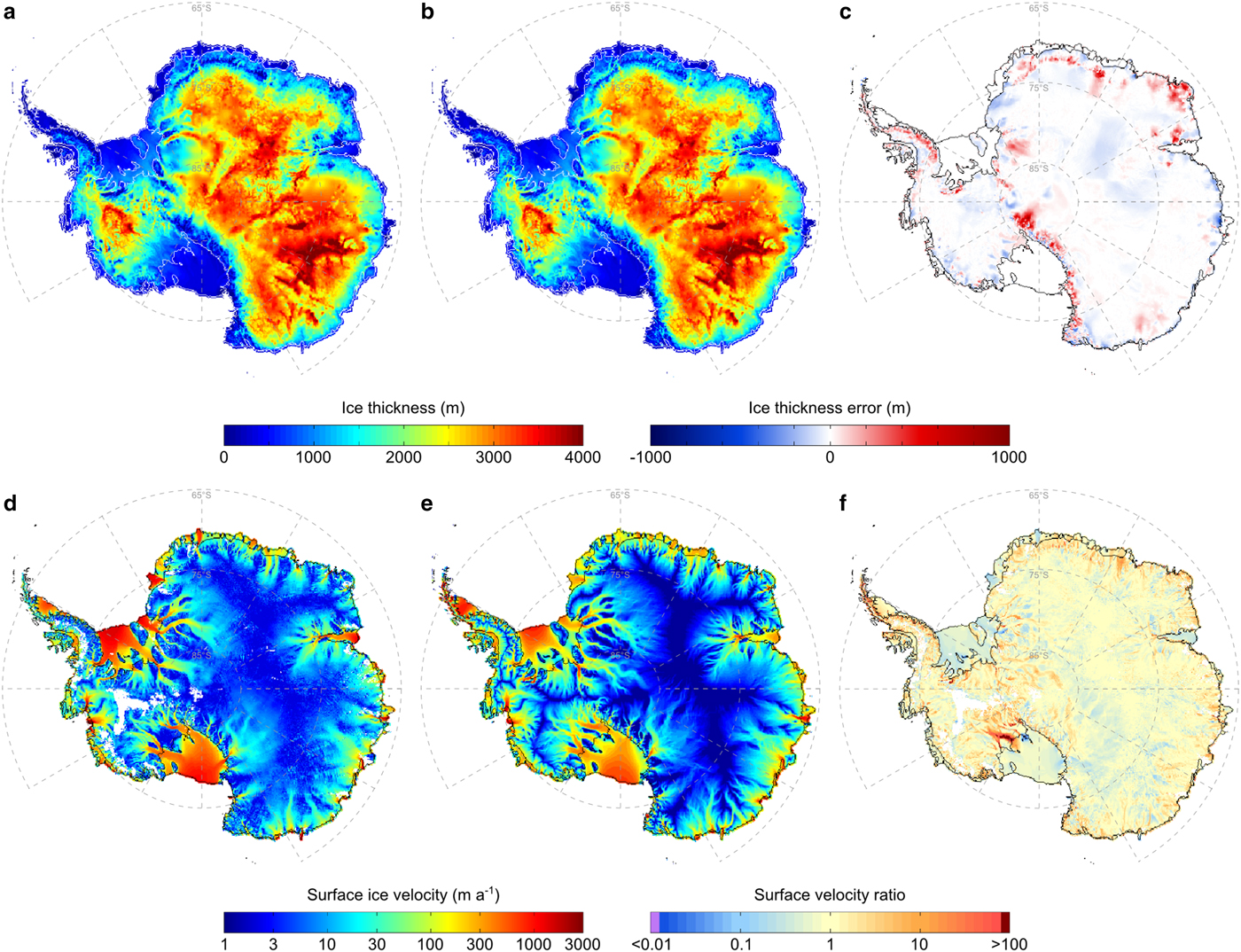
3. In contrast to the observation-based studies, our method does not employ an external dataset of the observed ice-surface velocities, but instead uses the ice velocity computed by the ice model. We compare the resulting ice-surface velocities to the observational dataset of Rignot and others (Reference Rignot, Mouginot and Scheuchl2011) (Fig. 2). General characteristics of the observed Antarctic ice flow are well reproduced by the model, particularly in areas of rapid ice flow and across the transition zones between slow- and fast-flowing ice sectors. The mean absolute difference between the observed and modelled surface ice velocities is 40.1 m a−1. The largest error occurs at the location of the former Ice Stream C (Fig. 2f), the existence of which is predicted by the model regardless of its stagnant behaviour over the last ~150 years (Hulbe and Fahnestock, Reference Hulbe and Fahnestock2007). Furthermore, ice velocities in some ice shelves (e.g. Ronne/Filchner, Amery and Stancomb–Brunt) are somewhat underestimated by the model, which we partly attribute to our choice of the ice flow enhancement factor in the computation of the SSA velocities (see Section 3.2). The computed ice velocities can also be affected by the assumption of an ice-sheet equilibrium with the present-day climate conditions, among other potential sources of uncertainty as discussed below. This may result in too-fast flow at the ice-sheet margins, especially near the observed ice stream locations (Bernales and others, Reference Bernales, Rogozhina, Greve and Thomas2017), requiring higher melting rates to account for the increased ice influx relative to observations. Figure 2 also shows the misfit between the modelled and observed ice thickness (Fretwell and others, Reference Fretwell2013), with a mean absolute ice thickness error being equal to 31.7 m. This misfit is significantly below the values that are usually found in modelling studies of the Antarctic ice sheet (Pollard and DeConto, Reference Pollard and DeConto2012), mainly due to the calibration of the basal sliding coefficients in the grounded ice sheet and of basal melting and freezing rates under the floating ice sectors. The largest ice thickness errors occur in mountainous regions, where basal thermal conditions do not favour ice sliding and the calibration is not performed (Bernales and others, Reference Bernales, Rogozhina, Greve and Thomas2017).
Top row: Comparison between the observed (a) and the modelled (b) Antarctic ice thickness distribution, in metres, together with the corresponding ice-thickness error (c), in metres. Observational ice-thickness data are taken from Fretwell and others (Reference Fretwell2013). Bottom row: Comparison between the observed (d) and the modelled (e) Antarctic ice-surface velocities, in m a−1, together with the ratio between the two (f), excluding very low velocities (<1 m a−1). Observational ice-velocity data are taken from Rignot and others (Reference Rignot, Mouginot and Scheuchl2011).
In addition to the effects of the neglected non-steady-state behavior mentioned above, deviations from the observation-based estimates may be partly explained by other limitations of our method. These include a relatively coarse resolution of the model (10 km) when compared with that of Rignot and others (Reference Rignot, Jacobs, Mouginot and Scheuchl2013) and Depoorter and others (Reference Depoorter2013) (1 km for ice thickness and 450 m for ice velocities) that also influences the location of the grounding line and ice-front flux gates. As described in Section 2, our model employs a hybrid combination of the SIA and SStA to compute the ice-sheet velocities, which could be affected by the lack of the higher-order dynamics (e.g. Gagliardini and others, Reference Gagliardini2013), especially across the transition zones near grounding lines. The magnitude of such influences will be hopefully assessed, as soon as similar experiments become feasible using higher-order models. Additional limitations arise from the uncertainties in the input datasets required by our model (e.g. the geothermal heat flux, climate forcing and bedrock topography) that influence the modelled ice-sheet dynamics and thus the estimates of the ice-shelf BMB, although the observational methods are also affected by the uncertainties in the topographic and climate data. Another limitation of both our model-based and observational methods is that they only provide estimates of basal melting and freezing rates for the present-day ice-shelf configuration, and the direct applicability of the retrieved values for scenarios with grounding-line migration driven by, for example, climate variations is not ensured (see Supplementary Materials). In the following sections, we present additional experiments that explore the influence of some of these limitations and uncertainties on the estimated ice-shelf BMB.
The large accretion zones retrieved along the Antarctic Peninsula, under big ice shelves (Ronne, Filchner, Ross East and Ross West), and at the East Antarctic coasts (mainly between the Stancomb–Brunt and Prince Harald ice shelves) are found to contribute + 214 Gt a−1 to our total BMB estimate, covering more than a quarter of the total ice-shelf area. This significant contribution to the total BMB is commonly disregarded by existing parameterisations of ice/ocean interactions (e.g. Beckmann and Goosse, Reference Beckmann and Goosse2003; Holland and others, Reference Holland, Jenkins and Holland2008). A potential workaround to compensate for the disregarded freezing would be to reduce the basal melt rates elsewhere to obtain an area-average value in agreement with observations. However, such option must ensure that the melt rates in key areas, such as grounding zones, are not significantly affected, to prevent artificial changes in the ice-shelf geometry.
Table 1 summarises our estimates of the ice-shelf BMB and the corresponding area-averaged melting rates. Major characteristics of the retrieved BMB are presented in the form of sector– and ice-shelf–averaged estimates, which allow for a direct comparison with previous estimates from other methods. Although the horizontal grid resolution used in this study is at the limit of what is currently feasible for whole-Antarctica forward modelling experiments, deviations from the ice-shelf areal extents presented in previous studies are inevitable, due to their higher resolution (~100 times). For many applications of ice-sheet models the grid resolution is very important, and we discuss it in a greater detail in the following section, where we present an analysis of potential sources of uncertainty on the reconstructed BMB of ice shelves.
Table 1 also presents the retrieved BMB for individual ice shelves, including the corresponding area-averaged basal melting rates. Average melt rates range from −4.2 (indicating freezing conditions under the Moscow University ice shelf, East Antarctica) to 46.5 m a−1 (indicating melting conditions under the Ferrigno ice shelf, West Antarctica), showing a similar variability to that found by Rignot and others (Reference Rignot, Jacobs, Mouginot and Scheuchl2013). Our model predicts local ice-shelf basal melting rates ranging from ~ −28 to ~ 103 m a−1. The minimum value marks the accretion under the Moscow University ice shelf, whereas the maximum value is detected at the grounding line of the Pine Island ice shelf. Freezing rates similar to those predicted at the base of the Moscow University ice shelf can be found elsewhere but only in isolated points, which most likely originate from an insufficient ice influx from the grounded ice sheet caused by the low model grid resolution (relative to the observation-based studies). To keep the ice-shelf thickness close to observed, the calibration scheme compensates for the lack of resolution through unrealistic basal freezing rates near the grounding line. Other potential model deficiencies arising from its limited resolution are discussed in a greater detail in Section 3.2. Numerous areas with very high melting rates (>25 m a−1) are found along the grounding lines of the Wordie, Ferrigno, Thwaites, Totten, Shackleton, Amery and Shirase ice shelves.
Grounding lines are known to exhibit melting rates that for many ice shelves are one-to-two orders of magnitude higher than area-average values (Rignot and others, Reference Rignot and Jacobs2002). Although some modelling studies have suggested sub-shelf melting rates with similar magnitudes (e.g. Payne and others, Reference Payne2007), the implementation of such high rates is not commonplace in large-scale, long-term ice-sheet modelling experiments. Our model-based results support the idea that ice flow models developed to study the dynamics of ice sheet-shelf systems may over-simplify and underestimate the influence of the ocean thermal forcing when parameterisations (e.g. Beckmann and Goosse, Reference Beckmann and Goosse2003; Holland and others, Reference Holland, Jenkins and Holland2008) are used. Although neither present-day observational data nor our estimates of melting and freezing rates can provide the necessary transient ice-shelf BMB for long-term simulations, our methodology and results can be used to aid the development of new parameterisations, which will be designed to fit the magnitudes and spatial patterns necessary to simulate the observed or hypothetical ice-sheet dynamical states under a variety of climate conditions.
3.2. Exploration of uncertainties
In this section, we present the results of modelling experiments that explore the influence of potential uncertainties in the input datasets and model formulation. We first analyse the sensitivity of the model results to a reduction of the model resolution in order to justify the use of a twofold lower resolution in our sensitivity tests relative to REF. Other than that, all presented experiments share identical model set-ups with the REF experiment (Section 2) presented in Figures 1 and 2, except for a change in the bedrock elevation boundary condition (BED simulation), geothermal forcing (GHF simulation) and climate forcing (ERA simulation). Furthermore, another set of simulations is carried out to assess the influence of a different basal sliding model, the use of a different hybrid scheme and a SIA-only model, and uncertainties in other model parameters on the modelled ice-shelf BMB and ice-sheet geometry. A summary of these sensitivity experiments is provided in Table 2.
Summary of the sensitivity experiments performed in this study, including: experiment name-code adopted in text, short description of the difference with respect to the reference experiment REF, number of figure(s) in text, horizontal grid resolution (Δx, y), mean absolute error in the ice thickness after equilibrium ( $\overline \Delta H$), total basal mass balance (BMB) and area-averaged basal melting rate (BMR). BMB and BMR values include equilibrium (left) and non-steady-state (right) values.
BMR values are in w.e., computed using a reference ice density of 910 kg m−3. All values are corrected for area distortions caused by the polar stereographic projection, following Snyder (Reference Snyder1987).
3.2.1. Influence of horizontal grid resolution
The computational expenses of the long-term, continental-scale simulation presented in Section 3.1 remain very high due to its relatively high horizontal resolution, and thus it is of interest to assess the influence of using a coarser, more viable model grid on the BMB estimates.
Figure 3 shows a comparison of the retrieved basal melting and freezing rates at grid resolutions of 20 and 40 km (henceforth GR20 and GR40, respectively). On the one hand, GR20 shows a strong similarity to REF, displaying only minor discrepancies mostly occurring in the proximity of grounding lines due to the smoothing effects of a coarser grid, which locally amplify melting and freezing beneath ice shelves (e.g. in the Larsen D and Amery ice shelves). On the other hand, GR40 exhibits the pronounced effects of a much coarser grid resolution in the form of considerably larger zones of melting and freezing. Although in some areas the retrieved BMB of ice shelves seems to be nearly insensitive to a fourfold decrease in resolution to each horizontal direction (e.g. the Bellingshausen and Amundsen Sea sectors), there are areas where melting predicted by the reference run REF is alternated by freezing in GR40 and vice versa. An example of such resolution-induced artefacts is the Amery ice shelf, where the area of high basal melting predicted near the grounding line by REF and GR20 has extended towards the ice-shelf front in GR40, overtaking the freezing zone detected at higher resolutions. In addition, new spots of strong accretion are retrieved, especially under big ice shelves and to the north of the Antarctic Peninsula. Interestingly, a few ice-sheet sectors in GR40 display inverted patterns relative to those predicted by higher-resolution simulations. For example, the Moscow University ice shelf shows a predominant melting, whereas an accretion prevails beneath the Cook East ice shelf, showcasing the strong effects of a very coarse grid resolution.
Results of experiments that employ different horizontal grid resolutions, including 10 km (top row), 20 km (mid row) and 40 km (bottom row). Ice thickness errors (left column) and surface ice-velocity ratios (mid column) as in Figure 2, although relative to REF. Estimated basal melting and freezing rates (right column) computed as the difference relative to REF (see Fig. 1).
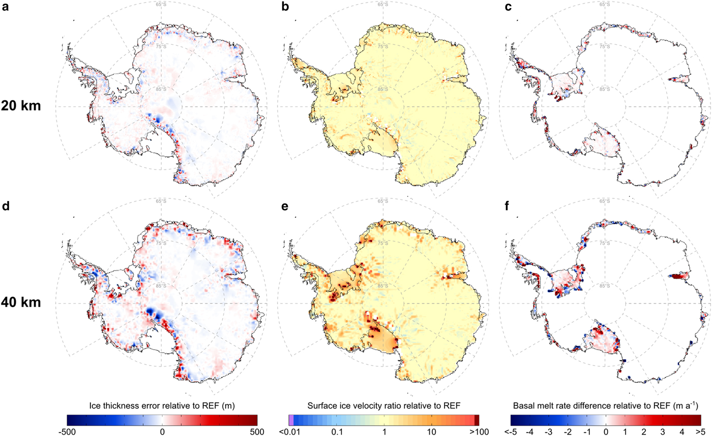
The use of a finer model grid improves the agreement between our BMB estimates and those of Rignot and others (Reference Rignot, Jacobs, Mouginot and Scheuchl2013) and Depoorter and others (Reference Depoorter2013) (Table 2 and Supplementary Materials), which we attribute to a more localised (i.e. smaller area per grid cell) adjustment of basal melt rates and thus a reduced amplification of their estimated values near grounding lines, together with a more accurate representation of small-scale features in the modelled ice influx from the grounded ice sheet. Consequently, we expect that the use of grid resolutions higher than our reference resolution (10 km) will further reduce these discrepancies. Our analysis suggests that the use of grid resolutions coarser than 20 km produces melting/freezing patterns and magnitudes that disagree with the results of higher resolution experiments and observation-based estimates, potentially leading to strong biases in ice-sheet simulations. Based on the good agreement between GR20 and REF, a resolution of 20 km is used in some of the numerous sensitivity tests presented in the next sections to reduce the computation time (see Table 2).
3.2.2. Influence of the input datasets
As described in Section 2, the experiments presented in this paper use the BEDMAP2 dataset as a reference topography against which the basal ice-shelf melting and freezing rates are calibrated. Here, we run a 20 km resolution experiment (henceforth BED) where the bed topography is perturbed within the estimated uncertainty bounds (Fretwell and others, Reference Fretwell2013) to assess potential impacts of such uncertainties on the retrieved BMB estimates. The perturbed bedrock is obtained by adding a randomly computed fraction of the uncertainty in the BEDMAP2 dataset to the reference topography (independently for each data gridpoint). The perturbation map has been smoothed in order to eliminate small-scale perturbations (below 100 km) that tend to introduce numerical instabilities due to artificially strong horizontal gradients. Differences between the reference and the resulting perturbed bedrock topography (Fig. 4a) reach up to ~500 m, with the largest discrepancies occurring mostly in the areas of East Antarctica where the BEDMAP2 dataset is based on gravimetric data only (Fretwell and others, Reference Fretwell2013). Compared with the experiment GR20, which is used here as a reference, the resulting ice-sheet equilibrium state has a smaller average absolute ice thickness error of 29.2 m (Table 2). This is due to a reduced overestimation of the modelled ice thickness over mountain ranges that we attribute to an enhanced ice drainage by new ice streams forming in areas where the bedrock topography has been lowered. This increment in the ice flow near the ice-sheet margins is also reflected in the new areas of ice-thickness underestimation (relative to GR20) surrounding the mountain ranges. An additional ice transport towards ice shelves increases the total ice-shelf BMB to a steady-state value of − 2282 Gt a−1, comparable with that of the GR40 simulation (Table 2), further demonstrating the strong impacts of the uncertainties in the topographic data on the estimated ice-shelf basal melting and freezing rates.
Results of experiments utilising a perturbed BEDMAP2 bedrock topography based on the uncertainty estimates of Fretwell and others (Reference Fretwell2013) (top row), a two-valued geothermal heat flow distribution of Pollard and DeConto (Reference Pollard and DeConto2012) (mid row), and the climate forcing from the ERA-Interim reanalysis (bottom row; Dee and others, Reference Dee2011). Thick black line in (d) represents the assumed division between East and West Antarctica. Left column shows the differences between the fields implemented in the above sensitivity tests and the REF experiment. Ice-thickness errors relative to BEDMAP2 (mid column) and estimated basal melting and freezing rates (right column) as in Figures 1, 2, respectively.
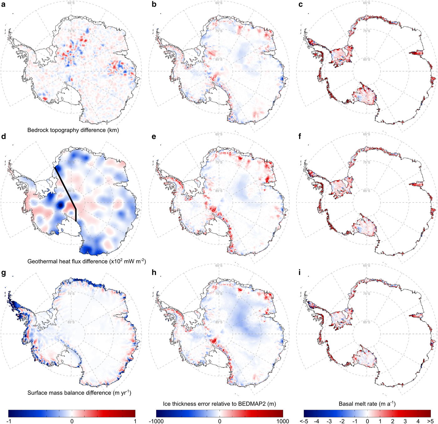
To test the influence of the uncertainties in the geothermal heat flux forcing, we perform a 20 km resolution experiment (henceforth GHF) featuring one of the simplest distributions commonly used in Antarctic ice-sheet simulations (e.g. Pollard and DeConto, Reference Pollard and DeConto2012). In this simulation we adopt two different values for West and East Antarctica, a lower value of 54.6 mW m−2 under the East Antarctic ice sheet, and a higher value of 70.0 mW m−2 across West Antarctica. In contrast to the BED simulation, the GHF experiment produces an average absolute ice thickness error of 34 m, which is close to that of GR20. Interestingly, the predicted total ice-shelf equilibrium BMB amounts to − 1468 Gt a−1 and increases to − 1742 Gt a−1 when the observed ice-thinning rates are considered, which falls within the error bounds estimated by Rignot and others (Reference Rignot, Jacobs, Mouginot and Scheuchl2013). Such decrease in the total BMB is explained by a comparatively lower geothermal heat flux (relative to Fox Maule and others (Reference Fox Maule, Purucker, Olsen and Mosegaard2005) in REF) in such areas as those located upstream of the Ross West and Ronne ice shelves in West Antarctica, and most of the ice-stream locations along the East Antarctic coast (Fig. 4d). In these areas, the use of lower values of geothermal heat flux decreases the sliding potential of ice streams feeding the ice shelves, thereby reducing ice velocities and generating lower ice-shelf basal melting rates near the grounding lines. Similar to the bedrock topography, uncertainties in the geothermal heat flux forcing strongly impact the retrieved basal melting and freezing rates under ice shelves, which compensate for the differences in the predicted mass flux across the grounding line.
Finally, the climate forcing from the ERA-Interim reanalysis (Dee and others, Reference Dee2011) is used in a 20 km resolution experiment (henceforth ERA) to test the influence of the uncertainties in the surface mass balance on the retrieved sub-shelf melting and freezing rates. The averaged precipitation rates and near-surface air temperatures are computed over the same period as the RACMO data (1979–2010) used in the REF experiment. A generally lower ice-sheet surface mass balance in the ERA-Interim dataset relative to RACMO (Fig. 4g) generates vast areas of an ice thickness underestimation, particularly in East Antarctica (Fig. 4h), producing a mean absolute ice thickness error of 44.3 m. In addition, the reduced ice accumulation generates lower ice-shelf basal melting rates, which are similar to the estimates from the higher-resolution REF experiment. Thus, in ERA more wide-spread accretion zones decrease the total ice-shelf steady-state BMB to a value of − 1687.5 Gt a−1. As described in Section 2.2, the RACMO model is forced at its boundaries by the ERA-Interim reanalysis, and therefore the discrepancies between the ERA and GR20 experiments can be largely attributed to the regional, polar-oriented features implemented in RACMO. The higher resolution of RACMO allows for better resolved topographic gradients and circulation patterns, which may be critical for the simulation of such processes as, for example, the drifting snow transport (Lenaerts and others, Reference Lenaerts2012). Despite these discrepancies, the differences between the ERA-Interim and RACMO datasets are small compared with the outputs of general circulation models (e.g. Agosta and others, Reference Agosta, Fettweis and Datta2015). Based on our results, we expect that model initialisation procedures driven by climate forcing from a variety of general circulation models would produce essentially different results in order to compensate for the discrepancies between the model-based climate datasets. An analysis of the differences between the resulting ice-sheet model initialisations may provide insights into potential internal biases of these climate forcing datasets. However, such analysis is beyond the scope of this study and is therefore deferred to future work.
3.2.3. Influence of the model formulation and parameters
As a complement to the simulations exploring the uncertainties in the input datasets, we present the results of experiments that aim to assess the influence of model complexity and model parameter choices on the inferred ice-shelf BMB. The hybrid combination of the SIA and SStA velocities presented in Section 2 (Eqn (1)) is a result of an original scheme formulation guided by our previous study (Bernales and others, Reference Bernales, Rogozhina, Greve and Thomas2017), where we compared the performance of different hybrid schemes during the calibration of an Antarctic ice sheet model. Among the tested hybrid combinations, the scheme based on the idea of Bueler and Brown (Reference Bueler and Brown2009) (henceforth HS-B) performed well in terms of the model fit to the observed ice-sheet thickness and ice velocities. However, HS-B showed a somewhat reduced ability to minimise the ice thickness errors in the continental interior of East Antarctica, because in this scheme the computation of the SStA velocities is mainly limited to the fast-flowing ice-sheet margins. We test the influence of the differences between our original scheme used in GR20 and HS-B by running a 20 km simulation using the latter. Our results show that these different hybrid schemes exhibit a similar performance in terms of ice thickness and ice velocities. The estimated ice-shelf basal melting and freezing rates from GR20 and HS-B are also in a good agreement, with some minor differences due to small discrepancies induced by the formation of isolated ice streams that produce a higher ice-shelf BMB of − 2094.2 Gt a−1 for HS-B. As shown by Bernales and others (Reference Bernales, Rogozhina, Greve and Thomas2017), the differences between hybrid schemes are masked by the calibration of the basal sliding coefficients. Since our computation of the ice-shelf BMB depends on the ice flux from the grounded ice-sheet sectors (and not on specific values of basal sliding coefficients), the results are only affected by the discrepancies between the modelled ice thickness and velocity fields from both schemes.
In Bernales and others (Reference Bernales, Rogozhina, Greve and Thomas2017) we also compared the performance of different hybrid schemes versus a scheme that uses only the SIA to model the grounded ice sectors (i.e. the SSA is used exclusively for the ice shelves) during the calibration of an Antarctic ice sheet model, showing that the latter approach produces larger misfits between the observed and modelled ice-sheet thickness and ice-surface velocities, especially near ice-sheet margins. Here we complement our sensitivity analysis by a comparison with this simpler approximation of the force balance equations, by performing an additional 20 km resolution experiment (henceforth SoS) using the above-mentioned SIA-only scheme. The increased mean absolute ice-thickness error of 48.8 m (Table 2) obtained from this experiment is accompanied by an even larger degradation of the estimated melting and freezing rates beneath ice shelves, producing a total steady-state BMB of − 2843.9 Gt a−1. Among all the experiments carried out in this study, the use of a SIA-only scheme for the grounded ice sectors has the largest impact on the retrieved ice-shelf BMB, stressing the need for a realistic treatment of the rapidly flowing ice-sheet sectors, where the SIA is no longer valid.
In this study, we ensure a good agreement between the modelled and observed ice-sheet thickness through the calibration of basal sliding coefficients that enter our reference sliding law. In this sliding model (see Bernales and others, Reference Bernales, Rogozhina, Greve and Thomas2017, Eqns (2)–(6)) basal velocities are assumed to be proportional to the third power of the basal shear stress (n = 3), but in principle other choices are possible. For example, the sliding model of Pollard and DeConto (Reference Pollard and DeConto2012) uses a weaker non-linear relation (n = 2) during the calibration of the basal sliding coefficients. Here we test the influence of such change in the sliding law on our results by performing a 20 km resolution simulation (henceforth SLD) using the set-up of Pollard and DeConto (Reference Pollard and DeConto2012), i.e. n = 2. The resulting ice-sheet thickness distribution is very similar to that from the GR20 experiment, with a slightly smaller mean absolute error of 32.8 m (Table 2) due to reduced ice thickness underestimations near ice-sheet margins. Similarly, the estimated ice-shelf steady-state BMB of − 2074 Gt a−1 in the SLD simulation is slightly higher by absolute value, due to locally higher ice-stream velocities in certain areas such as those found upstream of the Crosson and Dotson ice shelves. The similarity between our SLD and GR20 experiments suggests that a calibration of basal sliding coefficients can be, in principle, applied to any smoothly varying relation between the basal shear stress and the sliding velocities (Pollard and DeConto, Reference Pollard and DeConto2012).
Finally, our REF experiment uses a default value of E SSA = 0.5 for the ice flow enhancement factor for ice shelves, which falls within the range of values commonly used in Antarctic ice sheet simulations (0.3–1.0, e.g. de Boer and others, Reference de Boer2015). The use of this value results in ice-shelf velocities that are locally underestimated compared with the observational dataset of Rignot and others (Reference Rignot, Mouginot and Scheuchl2011), as shown in Figure 2. Here, we test larger enhancement factors to assess their impacts on the modelled ice-shelf velocities and basal melt rates, including E SSA = 1, E SSA = 2 and E SSA = 3 (Table 2). Compared with the REF experiment, the use of larger values of E SSA increases the internal ice-shelf flow, thereby reducing the basal melt (particularly near grounding lines) needed to compensate for the accumulation in areas where the ice shelves receive a high ice flux from the grounded ice-sheet sectors. Furthermore, an increasingly faster ice-shelf flow in this series of simulations reduces the misfit between the modelled and observed ice-surface velocities, from 40 m a−1 in the REF simulation, to 37 m a−1 (E SSA = 1), 34 m a−1 (E SSA = 2) and 32 m a−1 (E SSA = 3). Overall, the use of larger ice-shelf enhancement factors generates smaller total BMB estimates that are closer to those of Rignot and others (Reference Rignot, Jacobs, Mouginot and Scheuchl2013) and Depoorter and others (Reference Depoorter2013). Following the assumption that the ice flow enhancement factor for ice shelves should be ≤ 1 (Ma and others, Reference Ma2010), no special treatment of ice anisotropy in ice shelves (E SSA = 1) provides the best fit between our results and the cited studies. Since the same value is used across the grounded ice-sheet sectors (E SIA = 1, following the sensitivity analyses of Pollard and DeConto (Reference Pollard and DeConto2012) and Bernales and others (Reference Bernales, Rogozhina, Greve and Thomas2017)), we have concluded that this tuning parameter can be excluded from our particular model set-up.
We have also performed a series of experiments testing the influence of other model parameters (Table 2), such as: (1) degree-day and lapse-rate correction factors in the surface mass-balance model, ranging from 3 to 15 mm i.e. day−1 °C−1 for the former, and 6 to 10°C km−1 for the latter, and (2) the parameters related to the iterative adjustment of the ice-shelf basal melting and freezing rates (Eqn (3)). For our particular model set-up driven by the present-day climate forcing, these experiments have not shown any significant sensitivity to the tested parameter variations.
4. SUMMARY
This study presents equilibrium estimates of basal melting and freezing rates for the entire Antarctic ice-shelf system derived from an ice sheet-shelf model and present-day observations of the ice-sheet geometry. Our method is a model-based extension of the techniques presented in recent studies using the observed ice velocities and ice thickness to infer the ice-shelf BMB. In contrast, we derive the ice flow directly from an ice-sheet model calibrated against the ice-thickness observations and validated against the observed surface velocity field (Bernales and others, Reference Bernales, Rogozhina, Greve and Thomas2017). This approach allows for a detailed analysis of the BMB of ice shelves that are required by continental-scale, long-term ice-sheet models to reproduce the present-day geometry of the floating ice-sheet sectors. Our estimates complement previous glaciological and oceanographic reconstructions of the BMB of the Antarctic ice shelves.
The retrieved distribution of basal melting and freezing rates represents a total BMB steady-state estimate of −1648.7 Gt a−1, that increases to −1917.0 Gt a−1 when the observational ice-shelf thinning data from Pritchard and others (Reference Pritchard2012) are included. Our results exhibit similar patterns to those found by the observation-based study of Rignot and others (Reference Rignot, Jacobs, Mouginot and Scheuchl2013). In agreement with their reconstruction, we identify the highest ice-shelf basal melting rates near grounding lines and ice-shelf fronts, extensive accretion zones in-between under the biggest ice shelves, and high melting rates along the East Antarctic coasts suggesting that ocean thermal conditions there are similar to those detected in the Amundsen and Bellingshausen Sea sectors.
Additional experiments reveal that the use of a lower horizontal grid resolution tends to amplify the retrieved basal melting, thereby causing a significantly larger ice-mass loss from the Antarctic ice shelves. Since the misfit between our BMB estimates and those from the observational studies is reduced when an increasingly higher model resolution is employed, we anticipate that the use of even higher grid resolutions would further improve the agreement between the model-based estimates and the observational data.
Our estimates are insensitive to variations in the parameters controlling the iterative adjustment of the ice-shelf basal melting and freezing rates, and to changes in the degree-day and lapse-rate correction factors in the implemented surface mass-balance model. Similarly, variations in the basal sliding law and hybrid scheme formulation used to compute the grounded-ice velocities do not impose any significant changes in the predicted BMB of ice shelves. A choice of a flow enhancement factor larger than our reference value of 0.5 decreases the estimated basal melt rates near grounding lines and the misfit between the observed and modelled ice-surface velocities of large ice shelves, showing that a value of E SSA = 1 (i.e. no scaling of the ice-shelf flow) produces a total BMB estimate that is closer to the values obtained by Rignot and others (Reference Rignot, Jacobs, Mouginot and Scheuchl2013) and Depoorter and others (Reference Depoorter2013). Our experiments also show that uncertainties in the input datasets (topography, geothermal heat flux and climate forcing) hold the potential to strongly impact the retrieved ice-shelf basal melting and freezing rates by, for example, altering the ice flow patterns from the ice-sheet interior to its margins, and thus modifying the amount of ice mass that is routed towards the ice shelves across the grounding line.
Our model-based estimates reproduce well the complexity of the BMB of the Antarctic ice shelves, suggesting a strongly heterogeneous distribution of sub-shelf melting and freezing rates required by our model to fit the observed Antarctic ice-shelf geometry. Although these results cannot be directly implemented in freely evolving simulations with varying boundary conditions, they can be used as a first-order approximation to guide the development of effective parameterisations of the ice/ocean interaction for large-scale, long-term, prognostic modelling experiments.
SUPPLEMENTARY MATERIAL
The supplementary material for this article can be found at https://doi.org/10.1017/jog.2017.42.
ACKNOWLEDGEMENTS
We thank F. Pattyn and two anonymous referees for their very constructive comments that helped to improve this manuscript considerably. This work has been funded by the Helmholtz graduate research school GeoSim. IR was supported by the BMBF German Climate Modeling Initiative PalMod. We are very thankful to J.M. van Wessem for providing RACMO2.3 precipitation rate and near-surface temperature data and to J. Mouginot for providing the data necessary to reproduce their ice-shelf melting/freezing and thinning rates. All simulations were performed on the GFZ Linux Cluster GLIC.


 Open access