

Since McGuire (Reference McGuire1983) introduced the Gini coefficient to archaeology, many have assessed the method's accuracy in representing socioeconomic inequality through house size, namely as an index of labor investment (e.g., Fochesato et al. Reference Fochesato, Bogaard and Bowles2019; Kohler et al. Reference Kohler, Smith, Bogaard, Feinman, Peterson, Betzenhauser, Pailes, Stone, Prentiss, Dennehy, Ellyson, Nicholas, Faulseit, Styring, Whitlam, Fochesato, Foor and Bowles2017; Peterson and Drennan Reference Peterson, Drennan, Kohler and Smith2018; Smith et al. Reference Smith, Dennehy, Kamp-Whittaker, Colon and Harkness2014; Šprajc et al. Reference Šprajc, Marsetič, Štajdohar, Góngora, Ball, Olguín and Kokalj2022:25). The Gini coefficient summarizes inequality among a variable's values by measuring the area between the Lorenz curve (percentages cumulatively added from lowest to highest) and a hypothetical line of equality (see more in Analysis methods below). However, while mound-based residential datasets lacking stratigraphic information do not reliably index labor investment, final house dimensions may still represent the relative prestige (sensu Drennan et al. Reference Drennan, Peterson, Lu and Li2017) of occupants because structure size is visually impactful (Smith et al. Reference Smith, Dennehy, Kamp-Whittaker, Colon and Harkness2014:312). Put otherwise, occupation within large, impressive residences likely confers prestige on inhabitants, irrespective of when the actual phases of construction occur. This is especially salient for societal border zones, where mounded residential structures may result from diverse construction histories. The Rosario Valley, in modern-day Chiapas, was one such frontier, where waves of Maya immigrants from the Lowlands settled new centers or were integrated into pre-existing non-Maya polities (de Montmollin Reference de Montmollin1995; Pye et al. Reference Pye, Clark, Blake, Blake, Lee, Pye, Clark, Voorhies and White2016). This dynamic is similar to other Classic Maya frontiers, such as Copán (Richards-Rissetto Reference Richards-Rissetto2023).
Our research concerns the Late Classic (a.d. 700–900) house size inequality of three Maya polities in the Rosario Valley: Ojo de Agua, Rosario, and Los Encuentros. We generated Lorenz curves and Gini coefficients for five dimensions of house size across the three polities. Many of the sample's structures were multicomponent, but because we lack data on the degree to which they were constructed in the Late Classic period, we largely take their final forms as indices of prestige differentiation, not labor investment. Our analyses reveal that house size inequality in the region resembled that of contemporaneous Maya lowland cities. Intra-valley differences are also apparent, namely more house size equality for the smallest, shortest-lived polity (Los Encuentros), due mainly to the limited development of its apical elite architecture.
Dataset background
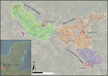
Ojo de Agua, Rosario, and Los Encuentros were Classic Maya polities in the Greater Rosario Valley, an upper tributary of the Grijalva River, located in southeast Chiapas (Figure 1; de Montmollin Reference de Montmollin1995:22–23). The Greater Rosario Valley has two upper branches in the east, opening to a wide valley bottom in its west. Before Mayas settled the Rosario Valley, it was inhabited by Mixe-Zoqueans (or “Mizoques”), whose material culture demonstrates clear ties to the Olmec site of La Venta (Bachand and Lowe Reference Bachand, Lowe, Lowe and Pye2012; Clark Reference Clark, Ruiz, Iglesias Ponce de León and Martínez2001, Reference Clark, Sharer and Traxler2016; Clark and Hansen Reference Clark, Hansen, Inomata and Houston2001; de Montmollin Reference de Montmollin1995:36; Lee and Clark Reference Lee and Clark2016; Lowe Reference Lowe and Adams1977, Reference Lowe, Blom, Ochoa, Lee and Kislak1983; Pye et al. Reference Pye, Clark, Blake, Blake, Lee, Pye, Clark, Voorhies and White2016:439).
Map of the Rosario Valley; the sampled Late Classic Maya polities with de Montmollin's survey boundaries in white, house group points in red, and structure outlines in black. Sources: ArcGIS Pro “Imagery” basemap, Maxar; de Montmollin 2018.

A major cultural shift occurred in the Late Preclassic (300–50 b.c.), when many settlements containing lowland Maya materials emerged amidst a handful of earlier centers, due to widespread migration from the Peten (Pye et al. Reference Pye, Clark, Blake, Blake, Lee, Pye, Clark, Voorhies and White2016:440). After this initial Maya expansion, there was a demographic contraction in the Early to Middle Classic periods (a.d. 200–650; Pye et al. Reference Pye, Clark, Blake, Blake, Lee, Pye, Clark, Voorhies and White2016:445). Then the maximum population was reached in the Late to Terminal Classic (a.d. 650–1000), when more Maya immigrants from the Lowlands moved into the region (Agrinier Reference Agrinier, Blom, Ochoa, Lee and Kislak1983; Pye et al. Reference Pye, Clark, Blake, Blake, Lee, Pye, Clark, Voorhies and White2016:450; Wells Reference Wells2015). This influx resulted in the cultivation of agriculturally marginal hillsides (de Montmollin Reference de Montmollin1995; Pye et al. Reference Pye, Clark, Blake, Blake, Lee, Pye, Clark, Voorhies and White2016:424). The area remained ethnically and linguistically diverse well into Spanish colonial times (Campbell Reference Campbell1988:267–270). Although this wave of immigrants possibly fled the decline of multiple lowland polities (Pye et al. Reference Pye, Clark, Blake, Blake, Lee, Pye, Clark, Voorhies and White2016:450), demographic collapse finally swept through the Rosario Valley between a.d. 900 and 1000 (de Montmollin Reference de Montmollin1995:3–4).
Several archaeological projects contributed to our dataset. Early investigations included limited survey operations in the 1950s and 1960s (Lowe Reference Lowe1959; Lowe and Mason Reference Lowe, Alden Mason and Willey1965; Shook Reference Shook and Sorenson1956; Sorensen Reference Sorenson and Sorenson1956). Thereafter, surveys and excavations of a 600 km2 area were conducted along the Grijalva River (Con Uribe Reference Con Uribe1981; Gussinyer Reference Gussinyer1973; Martínez Muriel and Navarrete Reference Martínez Muriel and Navarrete1978). Another larger survey (area: 2,600 km2) followed between 1973 and 1983 (Blake et al. Reference Blake, Lee, Pye, Clark, Voorhies and White2016; Bryant Reference Bryant1981; Lee Reference Lee1984). These studies were supplemented by de Montmollin's (Reference de Montmollin1987, Reference de Montmollin1989a, Reference de Montmollin1989b, Reference de Montmollin1995) systematic, intensive, full-coverage pedestrian surveys of the Greater Rosario Valley, specifically in 1983, 1988, and 1990 (survey area: 150 km2). His data were later digitized for public use (de Montmollin Reference de Montmollin2018). Among the three polities sampled from this dataset for our study, all residential structures have Late Classic components and we lack information on which have earlier components.
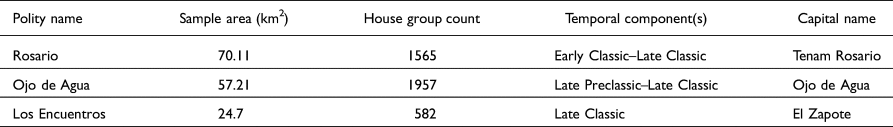
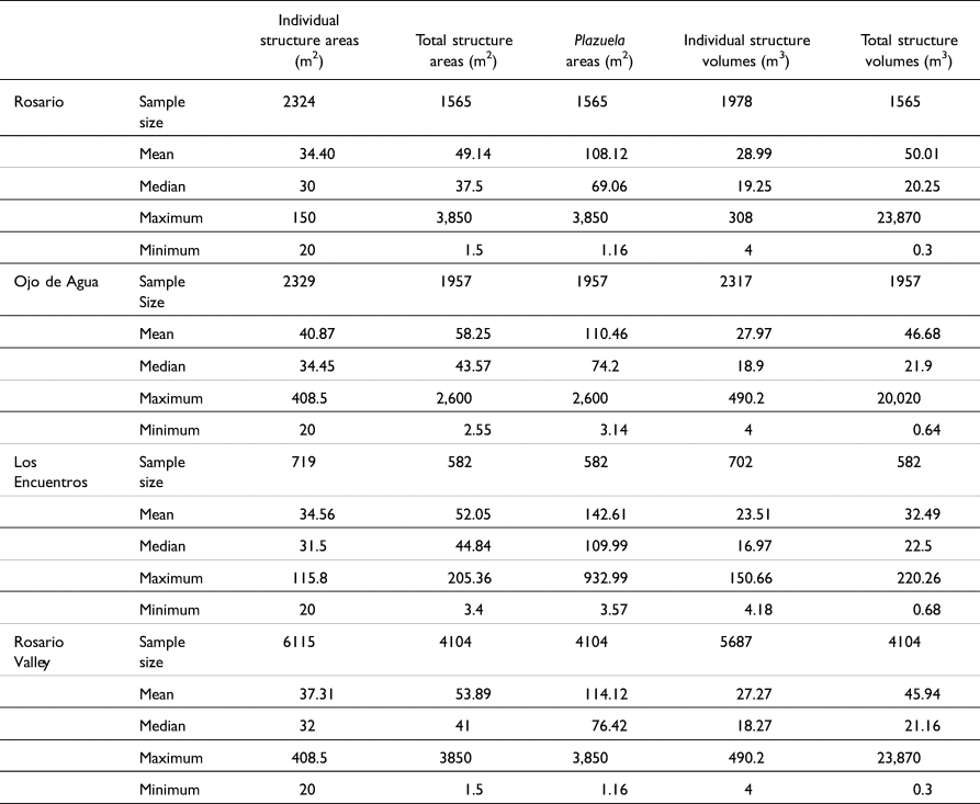
The largest polity and study area (70.11 km2) was Rosario, which reached its maximum extent in the Late Classic period, but had an Early Classic (a.d. 200–500) component (Agrinier Reference Agrinier, Blom, Ochoa, Lee and Kislak1983; Pye et al. Reference Pye, Clark, Blake, Blake, Lee, Pye, Clark, Voorhies and White2016:445). Its capital, Tenam Rosario, was erected on a hilltop separate from the established settlement (de Montmollin Reference de Montmollin1989a, Reference de Montmollin1989b, Reference de Montmollin1995:220). We sampled 1,565 house groups within the study area (Table 1). Rosario was probably in conflict with the neighboring Ojo de Agua polity (de Montmollin Reference de Montmollin1995:193), which was located at a lower elevation in the flatter, wider portion of the valley floor to the west. In contrast to Rosario, Ojo de Agua's eponymous capital was occupied from the Preclassic and was surrounded by settlement (de Montmollin Reference de Montmollin1995:107, 220). Ojo de Agua's survey area was 57.21 km2 and contained 1,957 sampled house groups. The Los Encuentros polity's study area, immediately to the south of Rosario, was smaller (24.7 km2) and included 561 sampled house groups. El Zapote was the main civic-ceremonial center of Los Encuentros, and likely purely Late Classic (a.d. 700–900; de Montmollin Reference de Montmollin1995:220).
Summaries of each polity.
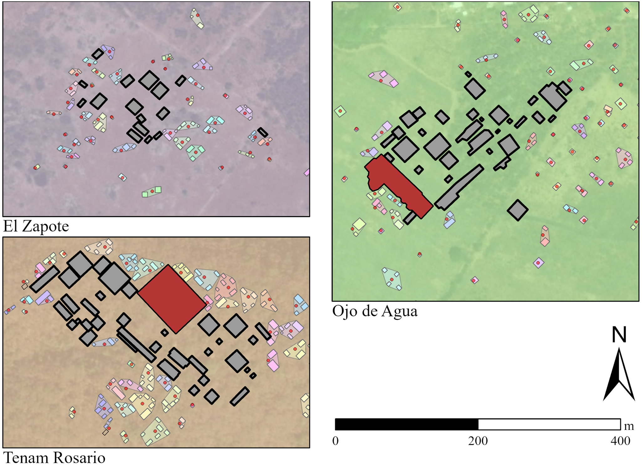
The 2018 dataset consists largely of measurements and polygons for all recorded structures. Although house group quantities for each “site” were noted, these clusters were originally not denoted on maps, and many of them contained dozens of structures. Consequently, and to assure consistency with others in this Compact Special Section, we designated our own house groups (Table 1), placing a point for each group according to structure location and other contextual data, then assigning structures to these points via nearest neighbor analysis (sensu Thompson et al. Reference Thompson, Walden, Chase, Hutson, Marken, Cap, Fries, Rodrigo Guzman Piedrasanta, Hare, Horn, Micheletti, Montgomery, Munson, Richards-Rissetto, Shaw-Müller, Ardren, Awe, Kathryn Brown, Callaghan, Ebert, Ford, Guerra, Hoggarth, Kovacevich, Morris, Moyes, Powis, Yaeger, Houk, Prufer, Chase and Chase2022). These groups likely represent households (Hammond Reference Hammond1975). House groups were typically supported by plazuelas, which are artificial patio surfaces (Ashmore Reference Ashmore and Ashmore1981a). Because house groups were identified remotely, we approximated plazuela areas by generating convex hulls that encompassed the structures of each group (Figure 2).
Maps of each polity's capital, with civic-ceremonial structures (not sampled) in grey, acropoleis in red, and surrounding house groups (opaque structures and semi-transparent plazuela convex hulls) distinguished by unique colors. Sources: ArcGIS Pro “Imagery” basemap, Maxar; de Montmollin Reference de Montmollin2018.
Analysis methods
We share our inequality analysis methods with all authors in this Compact Special Section (Chase et al. Reference Chase, Thompson, Walden and Feinman2023). Lorenz curves represent the inequality of a sample by cumulatively adding values (as percentages), arranged from lowest to highest to form a curve, plotted relative to a hypothetical line of equality. The Gini coefficient summarizes inequality as the area between the line of equality and Lorenz curve: the higher the value, the more unequal (Peterson and Drennan Reference Peterson, Drennan, Kohler and Smith2018). We ran these analyses for the following variables, sampled at polity- and valley-wide scales: individual structure area; total area of structures per house group; plazuela area; individual structure volume; and total volume of structures per house group. We could not estimate the volumes of plazuelas.
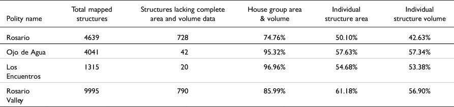
The total volume and area metrics for house groups include most domestic structures in de Montmollin's (Reference de Montmollin2018) dataset, in addition to two acropolis complexes from Ojo de Agua and Tenam Rosario. Acropolises are large, monumental platform complexes that contained civic-ceremonial structures and apical elite residences (de Montmollin Reference de Montmollin1995:70). Although these complexes were multifunctional, with many component structures serving domestic and public-facing purposes, they were predominantly elite residences (Folan et al. Reference Folan, Gunn, Domínguez Carrasco, Inomata and Houston2001; Inomata Reference Inomata, Ruíz, Ponce de León and Martínez Martínez2001:341; de Montmollin Reference de Montmollin1995:70, 93). Structures with incomplete area, volume, or height data were excluded from house group samples, where relevant. The plazuela area variable consists of convex hull areas for each house group and acropolis. Due to de Montmollin's dataset (Reference de Montmollin2018) only containing total area and volume for each acropolis (not for constituent structures) these complexes were not included in the individual structure samples. Relatedly, the platform volumes of acropolises could not be excluded from the total volumes of structures on these platforms, whereas comparable plazuela volumes could not be estimated for all other house groups; therefore, the house group volume Gini coefficient is inherently inflated. Finally, for consistency with other authors in this Compact Special Section (see Thompson et al. Reference Thompson, Chase and Feinman2023), we excluded structures smaller than 20 m2 in area from the single structure analyses. This is because mounds of 20 m2 or less may not have been standalone residences, instead serving ancillary domestic functions (Ashmore Reference Ashmore and Ashmore1981a:47, Reference Ashmore1981b:369; Hammond Reference Hammond1975; Webster and Gonlin Reference Webster and Gonlin1988; Wilk Reference Wilk1983). Given these differences, sample sizes varied widely according to variable (see Tables 2 and 3).
The quantities and proportions of total mapped structures for each polity.
Sample sizes and descriptive statistics for each variable.
Results
Confidence intervals (CIs) for corrected Gini coefficients in all samples varied widely, ranging between small intervals for individual structure areas (0.017) and massive intervals (0.300) for house group volumes (see Figure 3). Although the larger samples tend to have smaller CIs, the exceptionally large total structure volume CIs for Ojo de Agua and Rosario are due mainly to the inclusion of acropoleis. These palaces numbered only one per polity, dwarfing the next largest house groups.
Box-and-whisker plots for each polity-scale Gini coefficient. Created by authors.
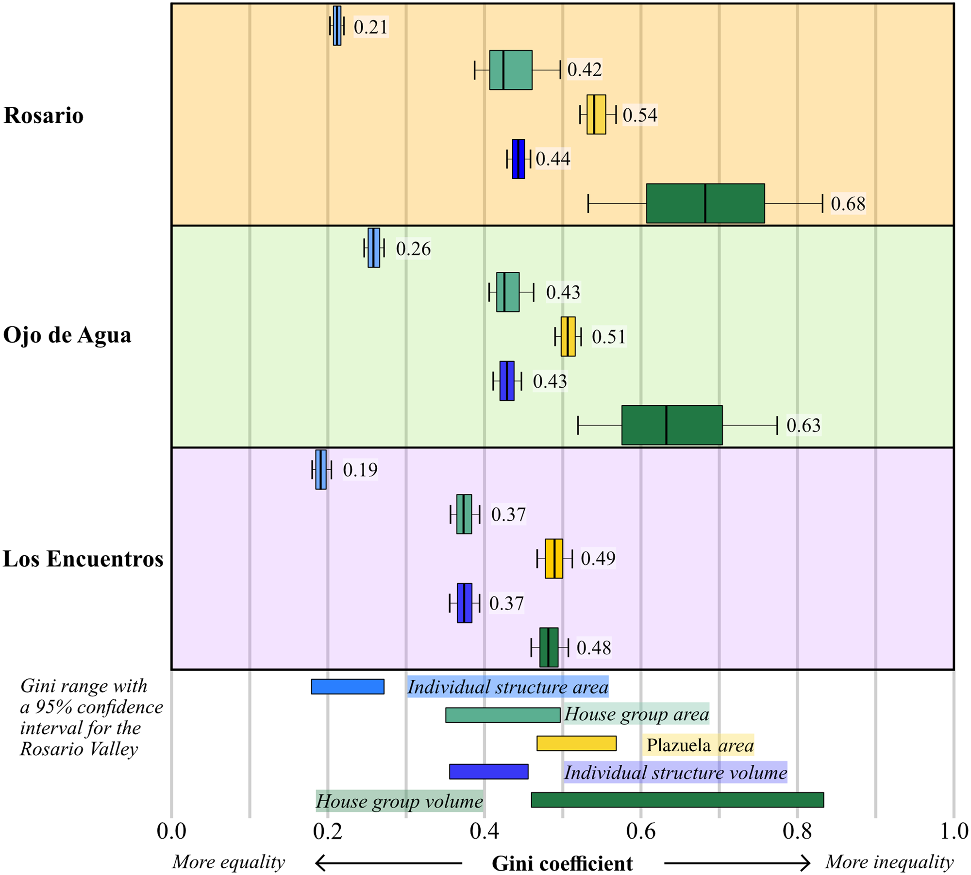
Overall, results show that Ojo de Agua and Rosario have the most unequal house size distributions, while those of Los Encuentros are more equal (Table 4 and Figure 3). The house group volume variables for Rosario and Ojo de Agua generated the highest Gini coefficients (0.68 and 0.63 respectively). As explained in the section above, these high values for house group volume were inflated by the inclusion of acropolis platforms. Rosario and Ojo de Agua's area-based samples also yielded higher Gini coefficients (0.21–0.54) than those of Los Encuentros (0.19–0.49). The exception is plazuela area, where Rosario's higher value (0.54) has no CI overlap with that of Ojo de Agua (0.51) or Los Encuentros (0.49).
Gini coefficient results.

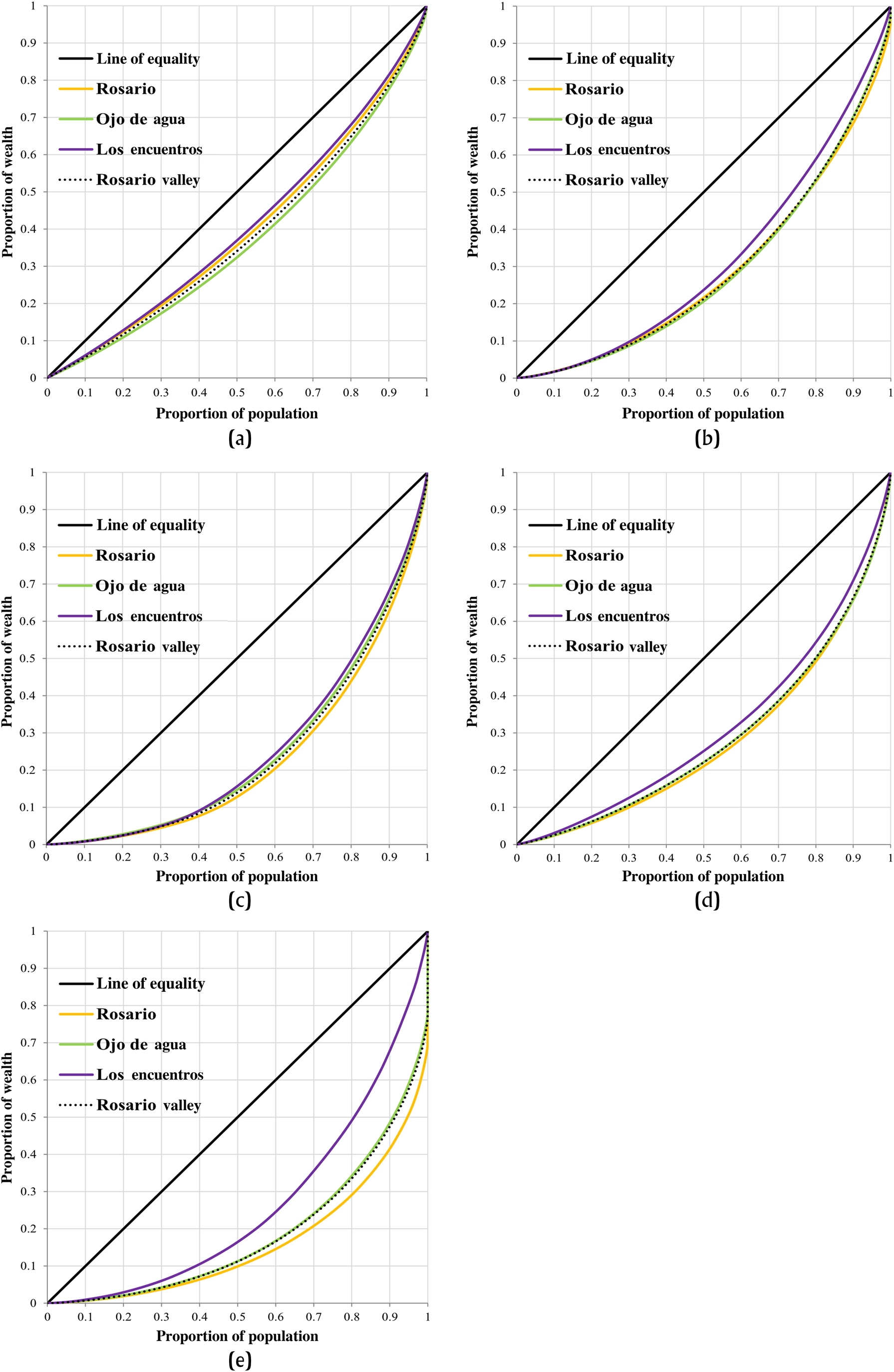
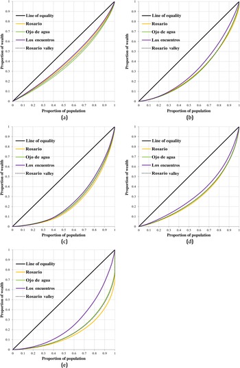
Finally, all Lorenz curves (Figure 4) were smooth, with no inflection points, except near the end. The biggest such jumps are visible in the Lorenz curves for house group volume. This pattern parallels the univariate plots that also show few substantial jumps in value, except towards the end of each curve. We have compiled our inequality data and house group polygons in an online dataset (Shaw-Müller and Walden Reference Shaw-Müller and Walden2023).
Lorenz curves for each variable: (a) structure area; (b) house group area; (c) plazuela area; (d) structure volume; and (e) house group volume. Created by authors.
Discussion
Before comparing and interpreting our results, it bears explaining what architectural inequality means in this context. Because we lack stratigraphic sequences for most domestic structures, their final, Late Classic forms only provide a snapshot of architectural inequality. Therefore, from an energetics perspective (Abrams Reference Abrams1994), their volume or area totals cannot represent labor investment and consequent socioeconomic inequality during specific periods. Yet the final Late Classic sizes of these structures still probably indexed prestige—that is, “esteem or respect in the non-economic sphere of social relationships” (Drennan et al. Reference Drennan, Peterson, Lu and Li2017:54) for those inhabiting them, regardless of when they were predominantly constructed. Indeed, the height of domestic structures had a “visual effect” (Smith et al. Reference Smith, Dennehy, Kamp-Whittaker, Colon and Harkness2014:312) that probably communicated prestige differentiation more than the labor necessary to build them. Furthermore, ethnoarchaeological evidence from Southeast Chiapas demonstrates that Maya residential architecture quality not only correlates with economic status, but also with social status (Blake Reference Blake, Lee and Hayden1988:51–54).
Irrespective of whether house size variables represent social status or wealth (as labor investment), our results still resemble existing Lowland Classic Maya inequality data. The lack of inflection points in the Lorenz curves corroborate prior claims that class-based social divisions were not prominent among Rosario Valley residences (de Montmollin Reference de Montmollin1995:293). That is, in keeping with lowland Maya samples, house sizes varied along a gradient, not according to distinct social ranks (Brumfiel Reference Brumfiel, Brumfiel and Fox1994; A. Chase Reference Chase2017:35–37, Reference Chase2021:249–250; D. Chase Reference Chase, Sabloff and Wyllys Andrews V1986:362; Chase and Chase Reference Chase, Chase, Robertson, Macri and McHargue1996, Reference Chase and Chase2011; Fash Reference Fash, Leventhal and Kolata1983; Freidel Reference Freidel and Ashmore1981; Hutson Reference Hutson2016:167, Reference Hutson, Hutson and Ardren2020:409–412; Masson and Pereza Lope Reference Masson, Lope, Lohse and Valdez2005; Pohl and Pohl Reference Pohl, Pohl, Brumfiel and Fox1994).
Another pattern for the Rosario Valley Gini coefficients is that the volume-based values (0.37–0.68) are higher than their area-based counterparts (0.19–0.54). Volume-based Gini coefficients are also high at other Classic Maya sites, ranging between 0.54 and 0.62 for Chunchucmil, Caracol, Uxul, Uxbenká, and Ix Kuku'il (Barnard Reference Barnard2021:144; Chase Reference Chase2017:37; Hutson and Welch Reference Hutson and Welch2021:820; Thompson et al. Reference Thompson, Feinman and Prufer2021:14). Copán yielded even higher volume-based Gini coefficient values than the Rosario polities, ranging between 0.65 and 0.85 (see Richards-Rissetto Reference Richards-Rissetto2023). In contrast, area-based Gini coefficients, such as those for plazuela area (0.34) at Caracol (Chase Reference Chase2017:37), house lot area (0.34) at Chunchucmil (Hutson and Welch Reference Hutson and Welch2021:820; Magnoni et al. Reference Magnoni, Hutson and Dahlin2012), and individual structure area (0.44) at Palenque (Brown et al. Reference Brown, Watson, Gravlin-Beman, Liebovitch and Braswell2012:318), are notably lower. Therefore, a key question is whether area-based or volume-based Gini coefficients more accurately reflect prestige differentiation.
In a region such as the Rosario Valley, where property sizes cannot be estimated (e.g., through houselots), area-based Gini coefficients are likely less reliable indicators of prestige and wealth differentiation. For example, ethnoarchaeological evidence from Chanal, a Maya community in southeast Chiapas, demonstrates that although the lowest- and highest-status households tend to have the smallest and largest area houses on average (respectively), this relationship is not linear for the rest of the sample (Blake Reference Blake, Lee and Hayden1988:54). That said, single structure area Gini coefficients were exceptionally low (0.19–0.26) for Rosario samples, with very tight confidence intervals, possibly, in part, for this reason and because they lacked acropoleis and small structures (less than 20 m2). Even if outliers were included, single structures would probably not represent household prestige differentiation because ancient Maya residences typically consisted of multiple structures, such as storage buildings, ancestral shrines, and kitchens (Hammond Reference Hammond1975; McAnany Reference McAnany2013; Sheets et al. Reference Sheets, Beaubien, Beaudry, Gerstle, McKee, Dan Miller, Spetzler and Tucker1990; Thompson et al. Reference Thompson, Feinman and Prufer2021). Indeed, among modern Maya communities in southeast Chiapas, at least 80 percent of households have separate kitchen structures (Blake and Blake Reference Blake, Blake, Lee and Hayden1988:40). Individual structure volume Gini coefficients are likely unrepresentative for similar reasons.
Likewise, plazuela area Gini coefficients (0.49–0.54) for the Rosario polities probably do not represent wealth or prestige differentiation. The Rosario polity has the highest plazuela area Gini coefficient value (0.54) because it has the largest area acropolis (3,850 m2) and smallest average plazuela areas. Ojo de Agua's plazuelas are just slightly larger, while those of Los Encuentros are much larger on average (Table 3). It bears emphasizing that because our plazuela area metric consists of convex hulls, it represents architectural size less well than estimates inferred from LiDAR or pedestrian mapping. Assuming convex hulls are accurate, however, the likeliest cultural explanation for the more spacious plazuelas of Los Encuentros is that, as multifunctional areas for everyday activities (Thompson et al. Reference Thompson, Feinman and Prufer2021:9; Vogt Reference Vogt2014:89), they benefit from more space to some extent, but there is a point at which plazuelas do not need to be larger to fulfill their social functions. Los Encuentros plazuelas could be so spacious and equal because many households simply had the room to expand their patios to socially useful maximums, whereas Rosario and Ojo de Agua residents did not. Therefore, the differences between Rosario Valley plazuela area statistics are probably not socially meaningful.
Of all variables, total structure volume by house group appears to yield Gini coefficients best reflecting prestige differentiation. Rosario and Ojo de Agua have much higher degrees of architectural inequality (with Gini coefficients for total structure area and volume ranging between 0.42 and 0.68) than Los Encuentros (0.37–0.48). Total house group volume is especially representative because it takes height into account (Smith et al. Reference Smith, Dennehy, Kamp-Whittaker, Colon and Harkness2014:312). Rosario and Ojo de Agua are more unequal for this variable (Gini coefficients: 0.68 and 0.63 respectively) than Los Encuentros (0.48) because their samples include acropolises, which are immense outliers that cause wide CIs. Furthermore, we can account for lower Gini coefficients at Los Encuentros by reference to its short-lived, strictly Late Classic settlement, where labor investments can be more reliably estimated. While Los Encuentros yielded the highest median value for total house group volume (22.5 m2), it also had the lowest mean (32.49 m2); therefore, most inhabitants probably grew their houses faster because they were not involved in monument-construction projects as ambitious as those of Rosario and Ojo de Agua. De Montmollin's (Reference de Montmollin1995:222) own analyses corroborate this hypothesis, demonstrating that Los Encuentros had the lowest proportion of elite architecture of the three polities.
Conclusion
The Gini coefficients and Lorenz curves for five dimensions of house size in the Rosario Valley samples demonstrate remarkable continuity with other Late Classic Maya polities: namely, a smooth gradient of architectural inequality and house group size Gini coefficients comparable to major Classic Maya centers in the Lowlands. Although the inequality of these three polities’ house size metrics is but a snapshot of architectural variability in the Late Classic, and so may only represent prestige differentiation in that period alone, aspects of economic inequality (via labor investment) can be gleaned from the Los Encuentros settlement, because it is a single component. Its sample yielded the most equal distribution of domestic architecture size in the valley, while also having the largest median for house group volume, probably because its apical elites levied less labor for monument construction. Therefore, political differences likely did exist between this short-lived Late Classic polity and the larger, well-established centers of Tenam Rosario and Ojo de Agua, for which labor investment data are more ambiguous. Relatedly, the diverse settlements of these older polities were probably characterized by more dramatic differences in household prestige, as reflected especially in the high Gini coefficient values of their visually impactful residential volume variables.
Acknowledgements
We thank Olivier de Montmollin for making the Upper Grijalva Basin dataset publicly available through the University of Pittsburgh's Comparative Archaeology Database. Likewise, we owe our gratitude to Alexander J. Martín, Hugo Ikehara, Weiyu Ran, and Faith Ruck for their work in designing and digitizing the dataset. As for the article itself, we are grateful to the three anonymous reviewers who generously offered insightful comments, improving both our analyses and prose. Finally, we are very thankful to Adrian Chase and Amy Thompson for organizing the 2022 SAA symposium in Chicago that led to this Compact Special Section, for providing the resources and guidance necessary to undertake these analyses, and for offering extensive feedback on this article.
Competing interests declaration
The authors declare none.
Data availability statement
All data will be made available through a publicly accessible online database (Shaw-Müller and Walden Reference Shaw-Müller and Walden2023).
Funding statement
Our research was made possible through funding from the University of Toronto, specifically for conference travel, stipends, and software licensing.


 Open access