





Introduction
Glacier ice velocities vary on daily to decadal time scales (Willis, Reference Willis1995; Quincey and others, Reference Quincey, Copland, Mayer, Bishop, Luckman and Belò2009; Rignot and others, Reference Rignot, Mouginot and Scheuchl2011; Armstrong and others, Reference Armstrong, Anderson and Fahnestock2017; Dehecq and others, Reference Dehecq2019; Shukla and Garg, Reference Shukla and Garg2020). Previous studies have reported seasonal changes in glacier ice velocities in mountainous regions like Alaska (Burgess and others, Reference Burgess, Forster and Larsen2013; Armstrong and others, Reference Armstrong, Anderson and Fahnestock2017; Vijay and Braun, Reference Vijay and Braun2017) and the Karakoram (Scherler and Strecker, Reference Scherler and Strecker2012; Usman and Furuya, Reference Usman and Furuya2018) as well as in polar regions (Rignot and others, Reference Rignot, Mouginot and Scheuchl2011; Moon and others, Reference Moon2014; Derkacheva and others, Reference Derkacheva, Gillet-Chaulet, Mouginot, Jager, Maier and Cook2021; Riel and others, Reference Riel, Minchew and Bischoff2021; Vijay and others, Reference Vijay, King, Howat, Solgaard, Khan and Noël2021; Qiao and others, Reference Qiao, Yuan, Florinsky, Popov, He and Li2023). One of the typical seasonal ice velocity signals reported in these studies consists of speedup with the onset of the melt season and subsequent slowdown with a recovery (minor speedup) in the early autumn season (Moon and others, Reference Moon2014; Vijay and others, Reference Vijay, Khan, Kusk, Solgaard, Moon and Bjørk2019; Nanni and others, Reference Nanni, Scherler, Ayoub, Millan, Herman and Avouac2023). Basal motion is reported to play a major role in the speedup of non-surge-type glaciers in melting periods, when the capacity of the subglacial drainage system to drain the meltwater is insufficient. Meltwater available with the onset of the melt season reaches the subglacial environment and pressurizes the subglacial system, which can further reduce basal friction and promote speedup (Bartholomew and others, Reference Bartholomew, Nienow, Mair, Hubbard, King and Sole2010; Andrews and others, Reference Andrews2014). As the melt season progresses, a reorganization of the system occurs as channels develop and become more efficient in routing the meltwater, which results in depressurization and glacier slowdown for the rest of the melt period (Nienow and others, Reference Nienow, Sharp and Willis1998). In autumn, creep closure dominates as melt inputs decrease, leading to a pressurization of the subglacial system and glacier speedup (Röthlisberger, Reference Röthlisberger1972; Shreve, Reference Shreve1972; Flowers, Reference Flowers2015; Benn and others, Reference Benn, Fowler, Hewitt and Sevestre2019).
Dehecq and others (Reference Dehecq2019) presented annual glacier ice velocities in High Mountain Asia (HMA) and found that annual ice velocities are correlated with the rates of mass change. They found that the glaciers showing negative mass change trends slowed down, whereas the glaciers showing positive mass change trends sped up on decadal time scales. However, they did not provide insights into the seasonality and associated mechanisms. Resolving seasonal ice velocities for glaciers in HMA has been a challenge because in situ observations are limited to a few weeks during the ablation season (Dobhal and others, Reference Dobhal, Kumar and Mundepi1995; Azam and others, Reference Azam2012; Patel and others, Reference Patel, Sharma, Singh, Pratap, Oulkar and Thamban2022), and the sensitivity and uncertainty of satellite remote sensing data and methods (Goldstein and others, Reference Goldstein, Engelhardt, Kamb and Frolich1993; Strozzi and others, Reference Strozzi, Luckman, Murray, Wegmüller and Werner2002; Heid and Kääb, Reference Heid and Kääb2012). A few previous studies have resolved seasonal velocity changes in mountainous regions (Quincey and others, Reference Quincey, Copland, Mayer, Bishop, Luckman and Belò2009; Burgess and others, Reference Burgess, Forster and Larsen2013; Satyabala, Reference Satyabala2016; Armstrong and others, Reference Armstrong, Anderson and Fahnestock2017; Usman and Furuya, Reference Usman and Furuya2018; Nanni and others, Reference Nanni, Scherler, Ayoub, Millan, Herman and Avouac2023). For instance, Usman and Furuya (Reference Usman and Furuya2018) investigated fast-moving eastern Karakoram glaciers using SAR (Synthetic Aperture Radar) offset tracking based on ALOS PALSAR-1 and -2 data and found increasing trends of summer and winter velocities. Following a similar SAR-based processing scheme, seasonal ice velocities were reported for three Himalayan glaciers (Satyabala, Reference Satyabala2016; Yellala and others, Reference Yellala, Kumar and Hogda2019). However, the subtle changes that may improve our understanding of changes on weekly to monthly time scales throughout the year in HMA and associated processes are largely unknown (Sam and others, Reference Sam, Bhardwaj, Kumar, Buchroithner and Martín-Torres2018; Vijay and others, Reference Vijay, Khan, Kusk, Solgaard, Moon and Bjørk2019; Derkacheva and others, Reference Derkacheva, Gillet-Chaulet, Mouginot, Jager, Maier and Cook2021). A recent study by Nanni and others (Reference Nanni, Scherler, Ayoub, Millan, Herman and Avouac2023) averaged a 7 year record of ice velocities of glaciers in the western Pamirs and showed glacier speedups in both summer and autumn seasons, with acceleration migrating upglacier in the melt season, possibly linked with subglacial drainage efficiency. Contrasting to most HMA glaciers, the Pamirs are known for many surge-type and fast-flowing glaciers ( $ \gt $100 m a $^{-1}$), which makes them relatively easier to capture using satellite remote sensing (Kotlyakov and others, Reference Kotlyakov, Osipova and Tsvetkov2008; Zhang and others, Reference Zhang, He, Hu and Liu2023).
In this study, we explore 6-day Sentinel-1 data over Drang Drung Glacier, located in the western Himalaya, for the year 2021. Sentinel-1 is not available everywhere in HMA with that frequency, providing a unique opportunity to study weekly to monthly scale ice velocity changes of a slow-moving mountain glacier with high precision. Our study uses a phase-based InSAR (Synthetic Aperture Radar Interferometry) method to compute 6-day velocities during autumn-winter periods, and intensity-based offset tracking to obtain monthly ice velocities during the summer period when the InSAR coherence is low. We combine these observations with the variation of Sentinel-1 radar backscatter intensity and channel width of the glacial stream estimated from Planet imagery, in order to provide insights into the possible factors driving seasonal ice velocity fluctuations. We further investigate the response of the glacier to seasonal meltwater inputs using a coupled numerical model to simulate the seasonal evolution of subglacial hydrology and ice velocity.
Study area
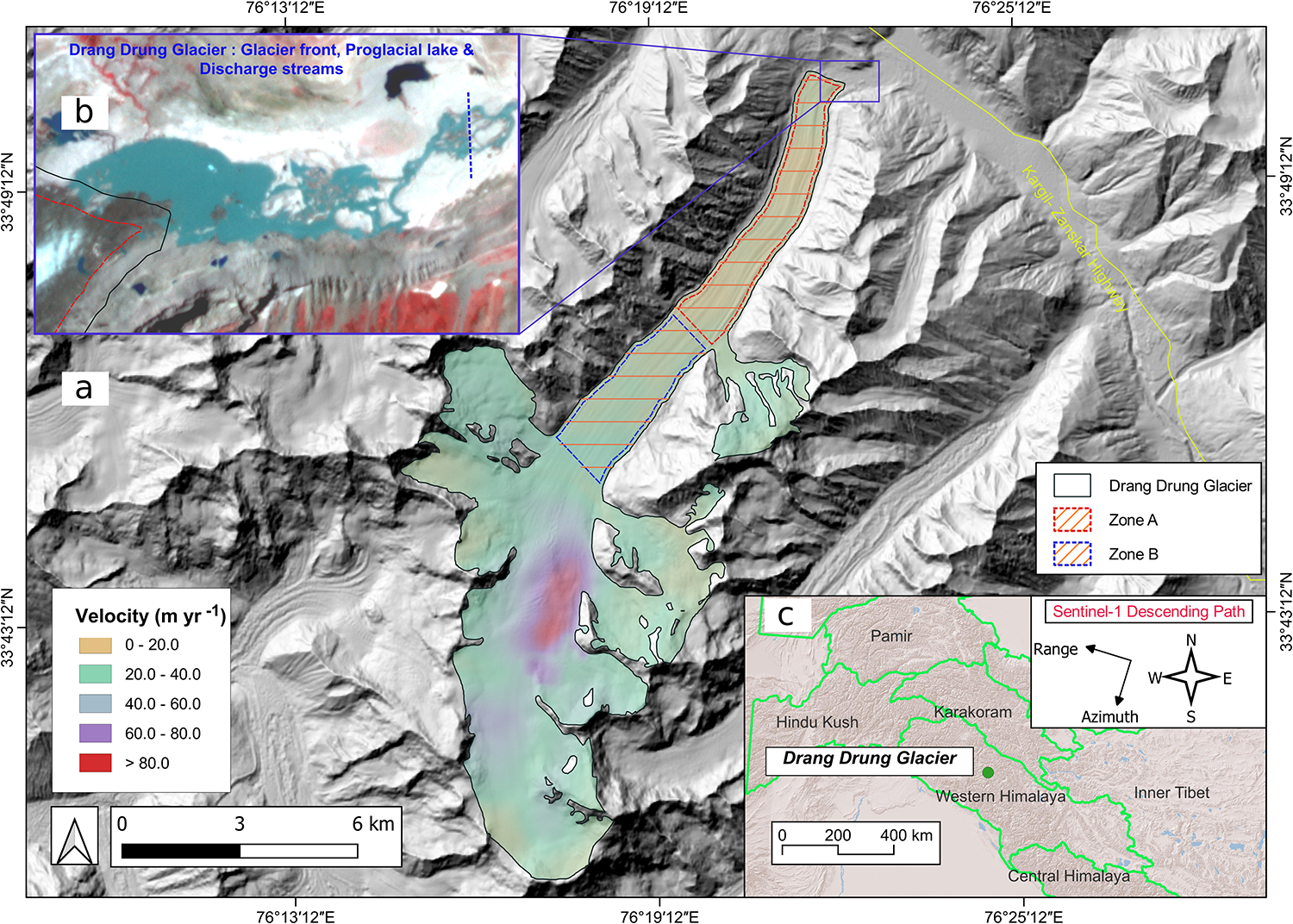
In this study, we observed intra-annual variations in glacier velocity on the Drang Drung Glacier (RGI60-14.18948; 33 $^{\circ}$45 $'$ N, 76 $^{\circ}$17 $'$ E), situated in the Zanskar Range of the western Himalaya, India (Fig. 1). Drang Drung Glacier is the second-largest glacier in the western Himalaya, extending from approximately 4100 m a.s.l. at its terminus to about 5600 m a.s.l. in its accumulation zone. The glacier drains into the Stod (Doda) River, a major tributary of the Zanskar River, thereby contributing to regional water security for downstream agrarian and pastoral communities. Recent satellite observations indicate an average retreat rate of 21.11 m a $^{-1}$ between 1971 and 2019 and a mean glaciological mass balance of $-0.74 \pm 0.43$ m w.e. a $^{-1}$ for 2021–23, highlighting the glacier’s pronounced sensitivity to ongoing climatic warming (Rashid and Majeed, Reference Rashid and Majeed2018; Azam and others, Reference Azam2025).
(a) Map of Drang Drung Glacier and its average annual velocity derived through SAR offset tracking based on Sentinel-1 GRD images acquired during May–October of 2021. (b) Zoom-in map shows the glacier terminus (adapted from RGI 6.0) and its proglacial lake, transect (blue dotted line) where the channel width is estimated. (c) Inset shows the location of Drang Drung Glacier in HMA and the Sentinel-1 descending path and its range, azimuth directions.

Methods
Velocity estimation from phase-based InSAR
We use 53 six-day Sentinel-1 Single Look Complex (SLC) InSAR pairs (Table S1, Supplementary) in descending mode from the year 2021 to construct short baseline interferograms using the Alaska Satellite Facility (ASF) Hyp3 Tool (Hogenson and others, Reference Hogenson, Arko, Buechler, Hogenson, Herrmann and Geiger2016). We use reference and secondary SLC images of InSAR pairs with a spatial baseline of less than 150 m and a temporal baseline of 6 days. The ASF’s Hyp3 Tool first converts SLC data into GAMMA Remote Sensing Software format by applying the calibration parameters related to orbit files and the backscatter values into the known scales (Agapiou and Lysandrou, Reference Agapiou and Lysandrou2020). After applying precise orbital data, scenes are coregistered using a normalized cross-correlation algorithm (Rosen and others, Reference Rosen2000), and an interferogram is generated. The interferogram has contributions from deformation ( $\phi_{defo}$), atmospheric delay ( $\phi_{atm}$), orbit error ( $\phi_{orb}$), DEM error ( $\phi_{dem}$) and noise ( $\phi_{noise}$) (Goldstein and others, Reference Goldstein, Engelhardt, Kamb and Frolich1993; Joughin and others, Reference Joughin, Winebrenner and Fahnestock1995; Reference Joughin, Kwok and Fahnestock1998). The orbital phase error is removed using ephemeris data. Assuming the same atmospheric conditions between short temporal InSAR observations, the atmospheric contribution to the phase data is neglected. A synthetic topographic phase is generated using the Copernicus 30 m Digital Elevation Model (DEM) (European Space Agency, 2021), and subtracted from the phase calculated in the interferogram to obtain the deformation phase in the Line of Sight (LOS) direction (Goldstein and others, Reference Goldstein, Engelhardt, Kamb and Frolich1993). The final LOS displacement contributions in the remaining phase are wrapped in 0– $2\pi$ radian values. The unwrapping of the phase is carried out by considering the highest coherence pixel (most stable point in the region) as a reference point and following the Minimum Cost Flow (MSF) algorithm (Eineder and others, Reference Eineder, Hubig and Milcke1998). Finally, the unwrapped phase is converted to LOS displacements by equation 1:
 \begin{equation}
\text{Phase} = \frac{4 \pi \, \Delta L}{\lambda} ,
\end{equation}
\begin{equation}
\text{Phase} = \frac{4 \pi \, \Delta L}{\lambda} ,
\end{equation}  $\text{where } \Delta L \text{is the path length difference, and } \lambda \text{is the wavelength.}$
Signal decorrelation in SAR can happen either spatially or temporally (Mattar and others, Reference Mattar, Vachon, Geudtner, Gray, Cumming and Brugman1998), and surface properties may seem to vary if they were seen from significantly different view angles or time periods, even if no true change has occurred (Goldstein and others, Reference Goldstein, Engelhardt, Kamb and Frolich1993; Woodhouse, Reference Woodhouse2017). InSAR coherence is a measure to estimate these signal decorrelations (Goldstein and others, Reference Goldstein, Engelhardt, Kamb and Frolich1993). We apply a coherence threshold of 0.5 on the glacier surface to select InSAR pairs based on manual inspection of several InSAR pairs and corresponding LOS displacements (Fig. S8). We find InSAR pairs during January–April and October–December on the glacier surface up to 12 km from the glacier terminus and are considered suitable for further processing and analysis.
Projection of LOS velocities into glacier flow direction
The displacement and subsequent velocity estimates using InSAR are measured in the radar LOS. In order to get the velocities in the actual flow direction of the glacier, ideally for a 3D displacement of the glacier, three independent non-coplanar measurements are required (Kwok and Fahnestock, Reference Kwok and Fahnestock1996). In this study, we assume glacier surface-parallel flow downwards the greatest slope (Goldstein and others, Reference Goldstein, Engelhardt, Kamb and Frolich1993; Kwok and Fahnestock, Reference Kwok and Fahnestock1996; Mattar and others, Reference Mattar, Vachon, Geudtner, Gray, Cumming and Brugman1998; Wangensteen and others, Reference Wangensteen, Weydahl and Hagen2005). The formula to project the ice velocity in the flow direction is given by
 \begin{equation}
V_g = \frac{V_{LOS}}{(\cos\alpha \sin\theta \cos\phi + \cos\theta \sin\alpha)},
\end{equation}
\begin{equation}
V_g = \frac{V_{LOS}}{(\cos\alpha \sin\theta \cos\phi + \cos\theta \sin\alpha)},
\end{equation}where  $V_g$ is the surface velocity in the flow direction of the glacier, $V_{LOS}$ is LOS velocity, $\theta$ is the look angle, $\phi$ is the aspect angle to the beam direction of radar and $\alpha$ is the glacier’s slope. These angles are calculated for a 100 m wide swath centered on the glacier centerline using the DEM and the satellite geometry data (Mattar and others, Reference Mattar, Vachon, Geudtner, Gray, Cumming and Brugman1998).
Velocity estimation from intensity-based SAR offset tracking
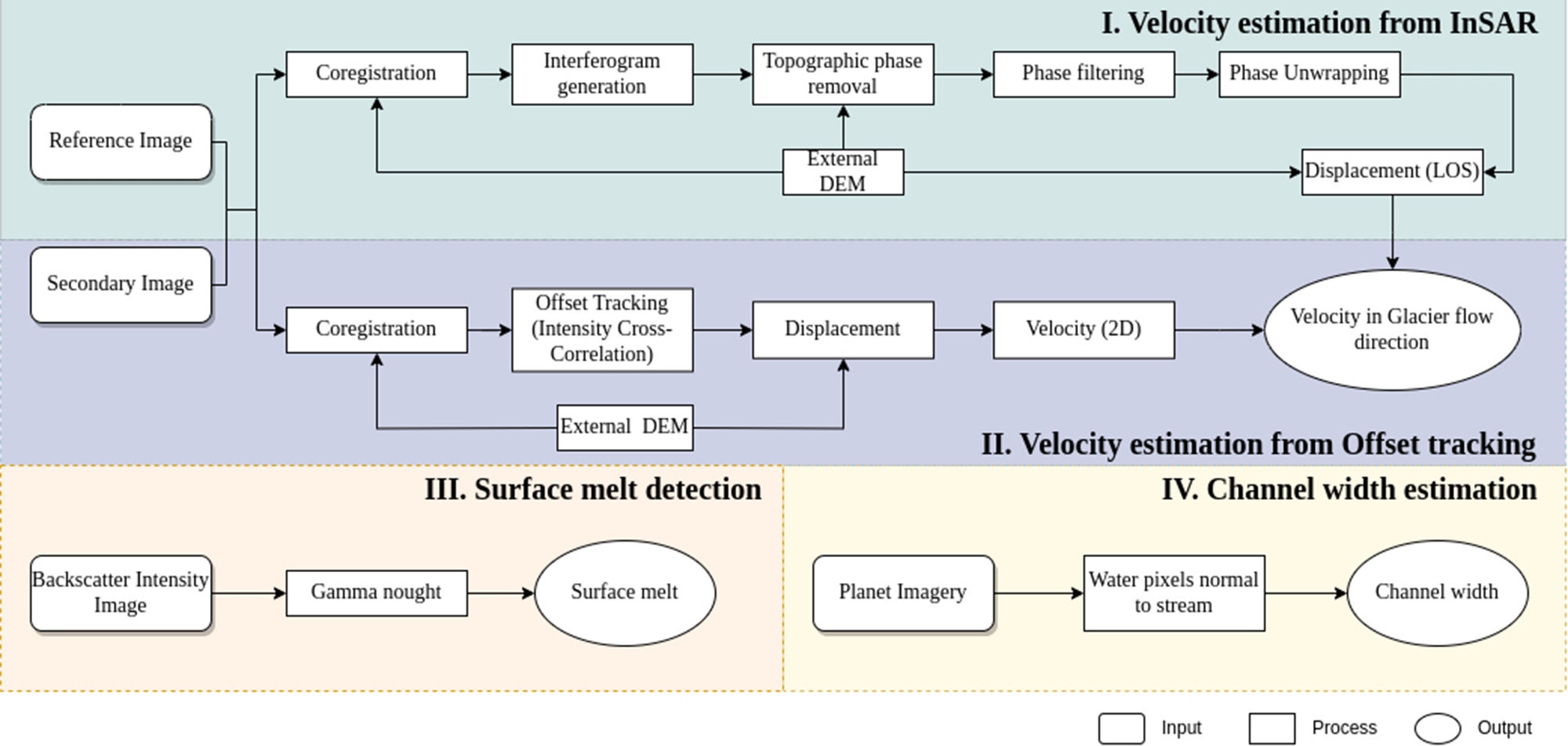
Glacier surface melting causes temporal decorrelation and loss of coherence of even 6 day InSAR pairs during the melt season. Therefore, we apply the SAR intensity-offset tracking method (Strozzi and others, Reference Strozzi, Luckman, Murray, Wegmüller and Werner2002; Reigber and others, Reference Reigber2013; Neelmeijer and others, Reference Neelmeijer, Motagh and Wetzel2014; Gomez and others, Reference Gomez, Arigony-Neto, De Santis, Vijay, Jaña and Rivera2019) on 6 Sentinel-1 descending Ground Range Detected (GRD) pairs (Table S2, Supplementary) that are separated by 24–36 days (Fig. 2). We process these scenes using the openly available Sentinel Application Platform (SNAP) software (available at http://step.esa.int). Because the intensity tracking only requires the SAR intensity information and the GRD scenes are already geolocated, fewer computational resources are needed when compared to the InSAR coherence approach. We perform the intensity tracking for Drang Drung Glacier and the nearby region by first coregistering image pairs using a Copernicus 30 m DEM with a normalized cross-correlation algorithm and cropping the images to a smaller extent to save computational time. Secondly, we define the search window size for the image comparison and set the normalized cross-correlation threshold to 0.1. After testing window sizes from 32  $\times$ 32 (range $\times$ azimuth) to 256 $\times$ 256, we find 256 $\times$ 256 to be the optimum for our study. This selection of window size is based on the size and possible speed of trackable features and the least offsets over stable terrain.
Flowchart to derive ice velocity, detect surface melt and estimate channel widths.

Retrieving seasonal ice velocity
We select 23 InSAR pairs out of the 53 six-day combinations available to compute the phase-based ice velocities. The pairs are chosen on the basis of high InSAR coherence and a high signal-to-noise ratio. Yet, most of the InSAR pairs rejected are from spring and summer, during which surface melting occurs, which often leads to decorrelation. Consequently, we only consider three pairs out of the six offset tracking pairs from the summer period. We choose pairs when the Normalized Median Absolute Deviation (NMAD) over off-glacier areas (noise) of the pair is either at the order of or less than the ice velocity magnitude of the glacier surface (signal). We extract the velocity values (both phase and intensity-based estimates) along the central flow line by taking the average of 4  $\times$ 4 neighborhood pixels. Afterwards, we fit these values using a locally weighted linear regression, called LOWESS (computed locally weighted scatterplot smoothing), to retrieve the seasonal trends with seasonal variations. The LOWESS fit was implemented in statsmodels Python package with a fractional smoothing parameter (frac) of 0.25 (Seabold and Perktold, Reference Seabold and Perktold2010). In the LOWESS fit, the closer data points in the time series have a higher weight in the fit compared to distant values (Cleveland, Reference Cleveland1979; Derkacheva and others, Reference Derkacheva, Gillet-Chaulet, Mouginot, Jager, Maier and Cook2021). We extract LOWESS fit interpolated velocities on a daily scale for the year 2021, then consider only significant signals to define the seasonal speedup (slowdown) if the change in consecutive velocity data retrieved by the LOWESS fit is more (less) than 1% of the annual median velocity at least for a week.
Proglacial lake channel width estimation
The discharge of a glacier is closely linked to the intensity of melting and therefore usually follows daily and seasonal cycles. The water emanating from the glacier primarily constitutes the glacier-wide mass balance flux due to melting, the main component of the ablation (St Germain and Moorman, Reference St Germain and Moorman2019). Due to the lack of meltwater discharge measurements from Drang Drung Glacier, we use the width of a braided portion of the stream draining Drang Drung proglacial lake as a proxy for the glacier discharge (Smith and others, Reference Smith, Isacks, Forster, Bloom and Preuss1995; Smith, Reference Smith1997; Alsdorf and others, Reference Alsdorf, Rodríguez and Lettenmaier2007) (Fig. 1). We utilized PlanetScope constellation’s optical multispectral images (Blue: 0.49 µm, Green: 0.565 µm, Red: 0.665 µm and Near-Infrared: 0.865 µm) with 3 m native spatial resolution in natural color and false color (NIR-Red-Green) compositions to estimate the effective channel width by counting the cumulative water pixels along a cross-section (at the transect shown in Fig. 1 of multiple streams approximately normal to the flow direction) using cloud-free Planet images during May–October 2021, covering most of the melt season (Table S4 and Fig. 3b).
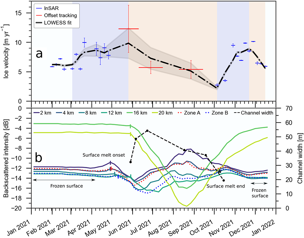
(a) Seasonal glacier surface velocity (m a $^{-1}$) of Drang Drung Glacier for the year 2021 (average of 0–12 km) with horizontal blue and red bars showing the epoch of observation and vertical blue and red bars showing the uncertainty in observation. The black dash-dotted line indicates the LOWESS fit of the observation, with the light blue block indicating the speedup, light orange block indicating the slowdown. (b) Seasonal variation in BI (dB) indicating frozen surface, surface melt onset (vertical line epoch indicating the sudden decrease in BI) at different distances from the glacier terminus and melt end (black star epoch on BI data) at 4600 m a.s.l. (personal communication, Irfan Rashid, 2023), the secondary $Y$-axis indicates the effective channel width of the streams draining from the Drang Drung Lake (black dashed line).

Detection of surface melt onset and melt period
To discriminate between the frozen and melting surfaces, we use the radar backscatter per unit area normalized for the local incidence angle. This data is provided by the Gamma naught products of Sentinel-1, which we obtained from ASF in a speckle-filtered Radiometric Terrain Corrected (RTC) version (Hogenson and others, Reference Hogenson, Arko, Buechler, Hogenson, Herrmann and Geiger2016). The backscattered intensity (BI) values (decibels or dB) are high when the surface is frozen and comparatively low in the presence of liquid water (Trusel and others, Reference Trusel, Frey and Das2012; Bevan and others, Reference Bevan, Luckman, Khan and Murray2015; Scher and others, Reference Scher, Steiner and McDonald2021). The spatial differences in BI along the glacier reflect elevation-driven contrasts in surface properties (Fig. S9). The upper accumulation zone shows a higher mean BI due to volume scattering in the dry or percolation zone, which drops quickly at melt onset and recovers following refreezing (Rau and others, Reference Rau, Braun, Friedrich, Weber and Goßmann2000; Marin and others, Reference Marin2020). Whereas the bare ice or wet snow exhibits a lower mean BI in the lower ablation area due to signal absorption (Rau and others, Reference Rau, Braun, Friedrich, Weber and Goßmann2000; Marin and others, Reference Marin2020). We map the frozen and the melting surfaces at different elevations over the glacier throughout the year 2021 (Figs. 3b and 4a and b). Sentinel-1 images are acquired over our study area in the early morning (local time: 05:00–06:00), when liquid water content in the snowpack remains low due to cooler overnight temperatures. Consequently, we expect backscatter intensity changes to lag behind actual melt onset and peak daytime temperatures, capturing delayed surface melt signals in our backscatter intensity observations (Scher and others, Reference Scher, Steiner and McDonald2021; Wendleder and others, Reference Wendleder2024).
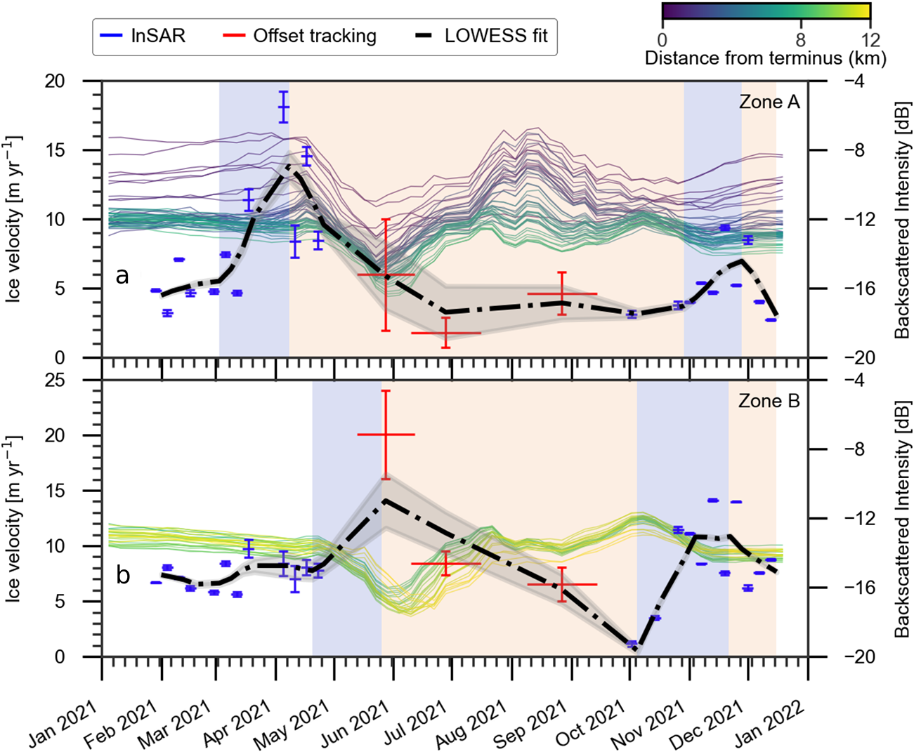
Intra-annual ice velocity of Drang Drung Glacier for 2021 for (a) Zone A, extending from the terminus to 8 km upglacier, and (b) Zone B, extending from 8 to 12 km upglacier, with the light blue block indicating the speedup, light orange block indicating slowdown in Zone A and Zone B, respectively, the secondary  $Y$-axis in both panels indicates the BI in dB, each colored line represents a point BI data along the centerline extending in (a) up to 8 km and (b) 8–12 km.

Ice velocity uncertainty estimation
Uncertainty in ice velocities derived from satellite remote sensing data can be estimated by analyzing the apparent velocity values in ice-free stable regions (Paul and others, Reference Paul2017; Vijay and Braun, Reference Vijay and Braun2017). We select stable areas of 2 km $^2$ near Drang Drung Glacier with slope values less than 14 $^{\circ}$ and InSAR coherence values greater than 0.5. Various statistical estimators (e.g. mean, median, etc.) have been proposed (Paul and others, Reference Paul2017; Gomez and others, Reference Gomez, Arigony-Neto, De Santis, Vijay, Jaña and Rivera2019; Pronk and others, Reference Pronk, Bolch, King, Wouters and Benn2021; Liang and Wang, Reference Liang and Wang2023), of which the median and the NMAD are less sensitive to outliers, while the mean and standard deviation are. We correct our ice velocity estimates with median values obtained over stable areas and consider NMAD as the uncertainty in ice velocity estimates.
Modeling subglacial hydrology and ice velocity
We simulate the seasonal evolution of subglacial hydrology and ice velocity at Drang Drung Glacier using the Subglacial Hydrology And Kinetic Transient Interactions model (SHAKTI; Sommers and others, Reference Sommers, Rajaram and Morlighem2018) coupled with the Ice-sheet and Sea-level System Model (ISSM; Larour and others, Reference Larour, Seroussi, Morlighem and Rignot2012). SHAKTI is a state-of-the-art subglacial hydrology model that calculates hydraulic head, effective pressure, water flux and geometry of the drainage system, accounting for spatially and temporally variable hydraulic transmissivity and transitions between laminar and turbulent flow regimes. SHAKTI has been previously applied primarily in the context of Greenland outlet glaciers (Sommers and others, Reference Sommers2023; Reference Sommers2024; Warburton and others, Reference Warburton, Meyer and Sommers2024) and is also well suited to simulate the hydrology of mountain glaciers (Narayanan and others, Reference Narayanan2025). SHAKTI is built into ISSM, a massively parallel numerical model with flexible options for simulating different aspects and processes of glaciers and ice sheets. The coupling between SHAKTI and the stress balance in ISSM occurs through the friction parameterization (i.e. sliding law), in which basal stress is a function of effective pressure (defined as the difference in ice overburden pressure and subglacial water pressure, calculated by SHAKTI) and ice sliding velocity (calculated by the stress balance in ISSM). In our simulations of Drang Drung Glacier, we use a vertically integrated higher-order approximation to calculate ice velocity (MOLHO; Dias dos Santos and others, Reference dos Santos T, Morlighem and Brinkerhoff2022) and a Budd-type sliding law (Budd and others, Reference Budd, Keage and Blundy1979). Constant and parameter values used in our modeling are documented in Table S3 in the Supplementary.
We take ice surface elevation from LEGOS and OMP (2025) and ice thickness estimated by Millan and others (Reference Millan, Mouginot, Rabatel and Morlighem2022), both shown in Fig. S4. We hold the glacier geometry steady, without dynamic thickening and thinning of the glacier. Boundary conditions in SHAKTI are prescribed as Neumann no-flux conditions along the lateral sides of the glacier and a Dirichlet boundary condition at the terminus outflow to the lake, setting hydraulic head so that the subglacial discharge pressure is equal to the hydrostatic pressure of the terminal lake, using a mean depth of 3.0 m based on bathymetry measurements (Ramsankaran and others, Reference Ramsankaran, Verma, Majeed and Rashid2023).
To generate the winter base state of the subglacial drainage system, we run one full year of stand-alone SHAKTI with zero meltwater inputs to the bed and zero velocity. In this winter spin-up, all water at the bed of the glacier is produced through basal melt. Beginning from this base state hydrological configuration, we then simulate two additional years of coupled winter spin-up, now solving for ice velocity through the stress balance in addition to evolving subglacial hydrology. This procedure results in steady converged hydrology and velocity fields for the glacier, representative of winter conditions, to serve as initial conditions for evolving transient seasonal forcing. Winter effective pressure and subglacial water flux are shown in Fig. S5. Simulated winter ice velocity compared to observed velocity is shown in Fig. S6.
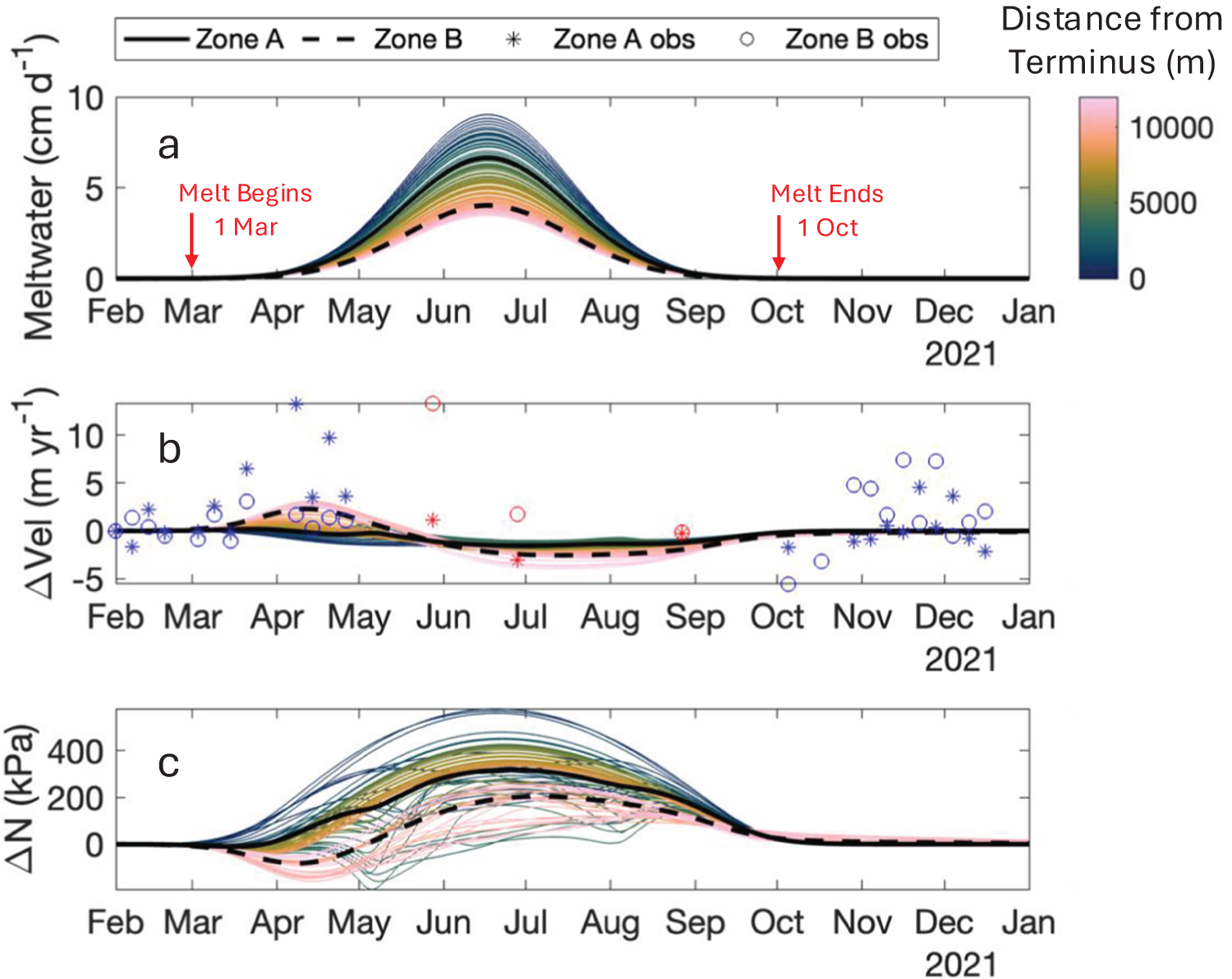
To explore the seasonal evolution of subglacial hydrology and ice velocity response at Drang Drung Glacier, we approximate seasonal meltwater inputs to the bed of the glacier with a smooth normal distribution curve (Fig. 5a). In this idealized seasonal forcing, melt onset occurs on 1 March and continues until 1 October, with peak melt on 16 June. The magnitude of melt varies with elevation, informed by an equilibrium line altitude of 5134 m a.s.l. and an ice ablation gradient of 0.62 m w.e. per 100 m elevation change (Azam and others, Reference Azam2025), following the ice ablation gradient method of estimating elevation-dependent variations in melt (Racoviteanu and others, Reference Racoviteanu, Armstrong and Williams2013).
(a) Idealized seasonal meltwater inputs to the subglacial system in Zones A and B. Each colored line represents a point in the model domain along the centerline extending 12 km from the terminus. (b) Modeled and observed change in velocity relative to velocity on 1 February at points along glacier centerline in Zones A and B. Blue markers represent velocities inferred from InSAR; red markers represent velocities inferred from feature tracking. (c) Modeled change in effective pressure relative to effective pressure on 1 February at points along glacier centerline in Zones A and B.

Results
Seasonal ice velocity variations of Drang Drung Glacier
In Fig. 3a, we show the seasonal velocity variations of Drang Drung Glacier in the year 2021 by averaging values over 12 km from its snout along its centerline. The average velocities range from 3  $\pm$ 0.24 m a $^{-1}$ (late summer minima) to 13 $\pm$ 4.01 m a $^{-1}$ (summer maxima). We divide the velocity time series into four distinct components, based on velocity variations (Fig. 3a); the spring/summer speedup (blue column), the summer slowdown (orange column), the autumn speedup (blue column) and the winter slowdown (orange column). The spring/summer speedup from 6 $\pm$ 0.20 to 13 $\pm$ 4.01 m a $^{-1}$ occurs from early March to late May 2021. The summer slowdown lasts for the rest of the melt season and the glacier attains its annual minimum velocity of 3 $\pm$ 0.24 m a $^{-1}$ in early October. The glacier quickly recovers (autumn speedup) and speeds up by about 300 % to 9 $\pm$ 0.27 m a $^{-1}$ during October–December 2021.
We further split the observed study area into two zones (based on spatiotemporal availability of InSAR coherence  $ \gt $ 0.5), Zone A (0–8 km from the terminus) and Zone B (8–12 km from the terminus), to show velocity variations as a function of upglacier distance and altitude (Fig. 4a and b). In general, the velocity variations in both zones show similar speedup and slowdown patterns, but they are distinct in terms of ice velocity magnitude and temporality. In Zone A, the spring/summer speedup occurs 5 weeks earlier than in Zone B, but the speedup signal lasts for a similar duration of $\sim$6 weeks in both zones. The summer slowdown in Zone A is relatively rapid during April–July; the velocities do not change much and are at the order of 3 m a $^{-1}$ until the end of October. However, the summer slowdown in Zone B is gradual and lasts for the entire melt season, reaching a minimum velocity of only $\sim$1 m a $^{-1}$. The subsequent autumn speedup in Zone B occurs about 1 month earlier than in Zone A. After attaining maximum autumn velocity, the velocity further declines in both zones and varies between 3 and 10 m a $^{-1}$ until the next potential early spring speedup.
Proglacial lake channel width variations
Figure 3b shows the variations in the width of streams coming out of the proglacial lake of Drang Drung Glacier during May–October 2021. This time series shows the rapid increase in effective channel width between late May ( $\sim$32 m on 29 May 2021) and late June ( $\sim$55 m on 23 June 2021). Afterwards, the channels consistently shrink for the rest of the observation period, with the minimum channel width observed in mid-October ( $\sim$19 m on 15 October 2021). Beyond this period, we did not have access to high-resolution cloud-free data to map channel widths.
Radar backscatter variations
Figure 3b shows the time-series BI values at various locations on the glacier surface along the central flowline. This time series is used to mark the frozen surface, and the onset of the melt season, at every location. In Fig. 3b, backscatter intensity (BI) values at higher-altitude sites ( 5300 m; 16 km and 20 km from the snout) range from  $-$3 to $-$5 dB (green and yellow lines) during winter. At 16 km, BI gradually declines from $-$3 to $-$16 dB (green line), marking the onset of the melt season, before recovering to pre-melt levels. The period of declination and recovery marks the melt period in these areas. BI values for downglacier (0–12 km from the snout) areas are slightly more complex. They do not fluctuate during winter and can clearly mark the frozen periods. A subsequent decline in BI values marking the onset are also clear, but the recovery and declination occur again in the melt period. It can be seen that the surface melt onsets downglacier (0–4 km) with a consistent migration upward. There is approximately a 2–3 week delay between Zone A (0–8 km) and Zone B (8–12 km) melt onset and this delay is increased to 4–6 weeks between downglacier (24 km) and upglacier ( $ \gt $16 km) areas (Fig. 3b).
Modeled seasonal evolution of subglacial hydrology and ice velocity
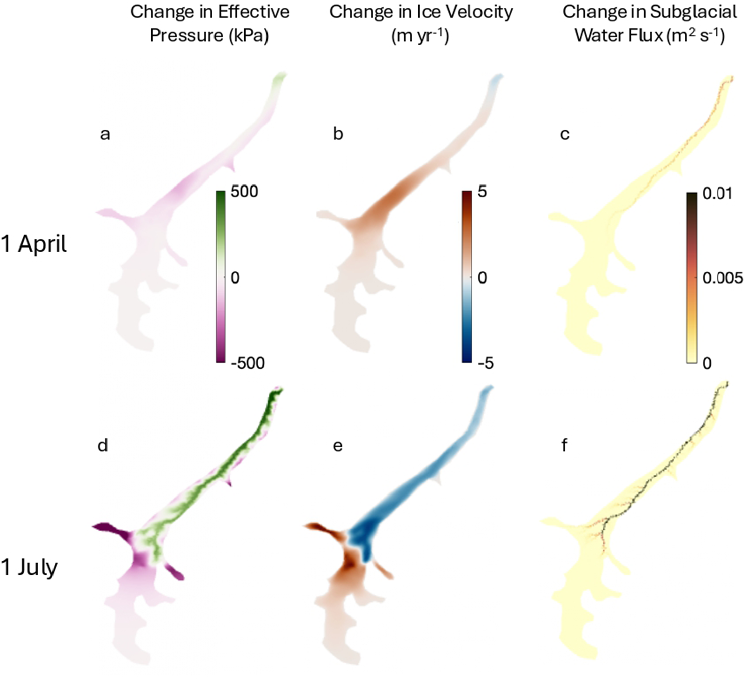
By forcing the glacier with idealized seasonal meltwater inputs to the bed (Fig. 5a), we simulate the seasonal evolution of the hydrological system at Drang Drung Glacier and corresponding ice velocity using the coupled model SHAKTI-ISSM. With the onset of meltwater reaching the bed on March 1, the glacier initially experiences a drop in effective pressure (i.e. increase in water pressure, with effective pressure defined as the difference between ice overburden pressure and water pressure at the bed) and accelerates (Figs. 5b and c, 6a–c and S7). As the subglacial hydrological system develops more efficient channelized drainage with higher capacity, effective pressure rises and velocity decreases through the summer (Figs. 5b and c and 6d–f). With decreasing meltwater inputs, the system again shuts down toward the end of the melt season, and a decrease in effective pressure corresponds to acceleration (Fig. 5b and c), equilibrating back to the winter base state. While the timing and magnitude of velocity changes differs from observations, the modeled seasonal pattern displays the salient features of spring acceleration, summer deceleration and fall acceleration of our observed velocity and provides insight into how the subglacial hydrology at Drang Drung Glacier evolves seasonally to produce the observed variations. To illustrate the spatial evolution of seasonal subglacial hydrology and ice velocity, Fig. 6 presents snapshots of modeled change in velocity, change in effective pressure and change in subglacial water flux on 1 April during the spring acceleration and 1 July during the summer deceleration. A decrease in effective pressure (i.e. increase in water pressure) corresponds to acceleration, with a less channelized drainage structure over most of the bed (i.e. more distributed drainage, and only one primary channel shown by high flux in Fig. 6c). The subsequent increase in effective pressure as more efficient channelization develops (i.e. decreasing water pressure) is responsible for the summer deceleration. This channel development appears as an arborescent network of high flux pathways in Fig. 6f.
(a) Modeled change in effective pressure relative to winter state during spring acceleration on 1 April. (b) Modeled change in velocity relative to winter during spring acceleration on 1 April. (c) Modeled change in subglacial water flux relative to winter state during spring acceleration on 1 April. (d) Modeled change in effective pressure relative to winter state during summer deceleration on 1 July. (e) Modeled change in velocity relative to winter during summer deceleration on 1 July. (f) Modeled subglacial water flux relative to winter state during summer deceleration on 1 July.

Discussion
Two episodes of speedup and slowdown at Drang Drung Glacier and connections to subglacial hydrology
The connections between basal motion due to subglacial channel efficiency and corresponding changes in surface ice velocities during the spring/summer have previously been reported in various glaciated regions across the world (Das and others, Reference Das2008; Quincey and others, Reference Quincey, Copland, Mayer, Bishop, Luckman and Belò2009; Schoof, Reference Schoof2010; Satyabala, Reference Satyabala2016; Armstrong and others, Reference Armstrong, Anderson and Fahnestock2017). Slow-moving glaciers like Drang Drung Glacier, or mountain glaciers in general, are known to be sensitive to meltwater availability and hence react quickly to shift from efficient to inefficient channels or vice versa (Kamb, Reference Kamb1987; Hewitt, Reference Hewitt2013; Nanni and others, Reference Nanni2020). At Drang Drung Glacier, we find two episodes of speedup and slowdown in 2021, which can be explained by meltwater-induced changes in the efficiency of the subglacial drainage system. The subglacial network of the glacier is not efficient at the beginning of the melt season. Meltwater inputs to an inefficient subglacial drainage system results in pressurizing the system and promoting basal sliding and speedup. The glacier speeds up for the first 3 months in the melt season and achieves its annual maximum. It then begins to slow down, indicating the development of subglacial channel networks and channelized flow of meltwater in a pattern that moves upglacier (Figs. 3 and 4). This evolution of efficient drainage during the summer is also supported by an almost two-fold increase observed in the effective width of the streams coming out from Drang Drung Lake during May–June, almost coinciding with the annual peak velocity (Fig. 3). We suggest a time lag of 4–6 weeks between the onset and duration of melt as observed by BI data and actual daytime temperatures (personal communications, Irfan Rashid, 2023), BI data being delayed in signal observations due to local time of acquisition and corresponding surface conditions.
We observe a clear upglacier migration of the speedup signal from Zone A to Zone B. Zone A begins to speed up in early March 2021, while the speedup in Zone B occurs approximately five weeks later, in late April. This temporal pattern is consistent with the upglacier migration of melt onset dates derived from BI data (Fig. 3b). However, the relationship between speedup and BI-derived melt onset differs between the two zones. In Zone B, the speedup is contemporaneous with the BI-derived melt onset in late April. In contrast, in Zone A, the speedup in March precedes the BI-derived melt onset by 4–6 weeks (Fig. 4a and b). We attribute this delay in Zone A’s BI signal to the local acquisition time of Sentinel-1 data. Our seasonal simulation results reproduce this acceleration migrating upglacier.
The glacier slowed down earlier in Zone A, with a sharp deceleration lasting 2.5 months followed by 4.5 months of sustained low velocity (totaling 7 months until next speedup) (Fig. 4). In Zone B, the glacier slowed down later in the season and for a shorter period (4 months until the next speedup), reflecting weaker drainage evolution. We expect that this earlier, more pronounced slowdown in Zone A results from intense, sustained meltwater input that rapidly establishes an efficient channelized system. These channels persist due to high cumulative discharge at lower elevations. In contrast, Zone B, which is near the ELA, experienced a later melt onset and lower input, leading to slower or incomplete channel development. Our model results agree with this elevation-dependent pattern, with elevations near or above the ELA (above Zone B) persisting in a state of acceleration throughout the melt season, as shown in Fig. 6c and f. Following the late-melt season minimum, the glacier at both zones speeds up in autumn for a duration shorter than the spring/summer seasonal changes. Zone B speeds up almost a month before Zone A. This pattern of higher elevations accelerating earlier than lower elevations following the late summer minimum is also reproduced in the model results (Fig. 5). As meltwater supply diminishes in the late melt season, subglacial channels close due to creep, leading to a slowdown. Subsequently, residual water stored in the glacier body, firn storage or supraglacial lakes repressurizes the distributed drainage system, triggering autumn speedup. Because ice is thicker in Zone B, overburden pressure causes channels there to close earlier than in downglacier Zone A, resulting in earlier repressurization and speedup in Zone B. This is supported by the ice thickness estimates of Drang Drung Glacier by Maanya and others (Reference Maanya, Kulkarni, Tiwari, Bhar and Srinivasan2016) and Millan and others (Reference Millan, Mouginot, Rabatel and Morlighem2022) (Fig. S4). Also, the magnitude of autumn speed-up in Zone B is greater than in Zone A, likely due to enhanced repressurization associated with thicker ice in Zone B. A weaker secondary slowdown is observed during winter (Fig. 4), which is likely influenced by limited velocity observations and reduced meltwater input to the glacier bed. The model simulates an acceleration in the fall that essentially returns to the winter background velocity. The observed minor deceleration in winter could be attributed to englacial or subglacial storage delaying the release of meltwater, which we neglect in these simulations. Because our velocity data do not extend into the following year, it remains uncertain whether this slowdown persists or transitions to a steady-flow regime (Figs. 3a, 4a and b and 5). While the match between the model and observation is encouraging, we note that there are quantitative differences with the model underestimating the magnitude of the speed up events, discussed below in Section 4.4.
Comparison with previous studies
Such seasonal variations throughout the year are yet unreported for any Indian Himalayan glacier, mainly because of lack and quality of data. With an average summer velocity of more than 20 m a $^{-1}$ over most of the ablation area (Fig. 1), our results agree with the existing study by Bhushan and others (Reference Bhushan, Syed, Arendt, Kulkarni and Sinha2018). However, there are no seasonal dynamics studies available to compare our velocities at Drang Drung Glacier in the rest of the seasons. Autumn speedup was previously observed in glaciers in Greenland (Moon and others, Reference Moon2014; Vijay and others, Reference Vijay, Khan, Kusk, Solgaard, Moon and Bjørk2019; Reference Vijay, King, Howat, Solgaard, Khan and Noël2021), Svalbard (Friedl and others, Reference Friedl, Seehaus and Braun2021) and the Pamir mountains (Nanni and others, Reference Nanni, Scherler, Ayoub, Millan, Herman and Avouac2023). Major reasons for autumn speedup are generally linked with additional water supply due to rainfall events (Schellenberger and others, Reference Schellenberger, Dunse, Kääb, Kohler and Reijmer2015), drainage of supraglacial ponds and remaining meltwater in the system (Hewitt, Reference Hewitt2013; Hart and others, Reference Hart, Young, Baurley, Robson and Martinez2022), which pressurizes the closing channels again. As we demonstrate in our modeling with an idealized seasonal meltwater input curve, however, the autumn speedup occurs even without additional rainfall events and can be explained by the pressurization of the subglacial system once the generally efficient channelized drainage system has reverted back to an inefficient distributed system.
Accuracy and error analysis
Field data for Drang Drung Glacier are not available in published studies to compare our short-term ice velocity changes. Here, we discuss our method uncertainties. The uncertainty in the velocity product by offset tracking method is mainly related to pixel co-registration (Pronk and others, Reference Pronk, Bolch, King, Wouters and Benn2021). This depends on the quality of the input data and varies from 1/10th to 1/20th of the pixel spacing (Scherler and others, Reference Scherler, Leprince and Strecker2008; Nanni and others, Reference Nanni, Scherler, Ayoub, Millan, Herman and Avouac2023). Under favorable correlation conditions, sub-pixel precision can reach 1/20 pixels or better (Strozzi and others, Reference Strozzi, Luckman, Murray, Wegmüller and Werner2002; Dehecq and others, Reference Dehecq, Gourmelen and Trouve2015; Friedl and others, Reference Friedl, Seehaus and Braun2021). The error (NMAD) in summer velocity products based on offset tracking is estimated as 0.59 cm day $^{-1}$ (NMAD $ \lt $1.1 cm day $^{-1}$ in all cases). Moreover, in offset tracking, the window size can significantly affect velocity estimates by balancing noise reduction and spatial resolution. We tested several window size combinations, ranging from 32 $\times$ 32 to 256 $\times$ 256, and finally chose the 256 $\times$ 256 window size that showed consistent seasonal spatial coverage of the ice velocity. However, this choice may have underestimated velocity values, especially in regions with high and local velocity values. For instance, offset-tracking results on neighboring glaciers (Figs S1–S3) initially reveal seasonal patterns similar to Drang Drung Glacier; however, after median-bias correction over stable terrain, summer velocities appear to be affected due to sparse temporal sampling and low signal-to-noise ratios. Consequently, these results are excluded from further analysis, limiting quantitative comparisons to Drang Drung Glacier. The error in the velocity product by InSAR corresponds to either misregistration, orbit, baseline, external DEM, phase unwrapping or atmosphere (Joughin and others, Reference Joughin, Kwok and Fahnestock1998). Phase unwrapping errors in ice sheets are found by large phase gradients (Werner and others, Reference Werner, Wegmüller, Strozzi and Wiesmann2002). The best way to reduce this error is to eliminate these phase gradients and use a better interferometric correlation by using small temporal baseline data (Joughin and others, Reference Joughin, Kwok and Fahnestock1998). We have used the precise orbit data and sorted the input data based on the suitable baseline parameters, and restricted the coregistration error to 1/10 of pixel size (Nela and others, Reference Nela, Bandyopadhyay, Singh, Glazovsky, Lavrentiev and Arigony-Neto2019); therefore, the remaining error sources are external DEM and atmospheric effects. Atmospheric errors are due to signal delays in the ionosphere because of the high concentration of electrons and troposphere because of the rate of change of water vapor (Luckman and others, Reference Luckman, Quincey and Bevan2007); these errors are unavoidable unless proper climate data is available and are typically less than 1 cm day $^{-1}$ (Mattar and others, Reference Mattar, Vachon, Geudtner, Gray, Cumming and Brugman1998). The InSAR-based velocity error (NMAD) in the projected direction of the glacier flow is estimated as 0.079 cm day $^{-1}$ (NMAD $ \lt $ 0.32 cm day $^{-1}$ in all cases). The aspect angle between the radar LOS and glacier flow direction is critical and induces uncertainties when the LOS velocities are not sensitive to the actual flow direction; this uncertainty increases from an aspect angle of 0 $^{\circ}$ to 90 $^{\circ}$ and decreases from 90 $^{\circ}$ to 180 $^{\circ}$ (Wangensteen and others, Reference Wangensteen, Weydahl and Hagen2005). The aspect angle in our estimates is found to be 57.92 $^{\circ}$. Therefore, our estimated velocities in glacier flow direction are moderately sensitive to LOS velocities derived from InSAR.
Differences between modeled and observed velocities
Our coupled SHAKTI-ISSM modeling provides insights into the general pattern of seasonal evolution of subglacial hydrology at Drang Drung Glacier, demonstrating that the modeled ice velocity response to seasonal meltwater inputs reproduces the summer deceleration trend as the subglacial drainage efficiency increases. This is the first application of the coupled model to a mountain glacier. We note several differences between the modeled and observed velocities presented in this paper, as shown in Figs. 5b, S6 and S7. First, modeled winter velocities are generally higher than observed, especially in the upper reaches of the glacier (Figs S6 and S7). This base velocity is influenced by model assumptions of ice temperature, which affects the rheology and corresponding viscosity, the friction coefficient representing roughness at the glacier bed or bed material type, and by velocity boundary conditions. Note that modeled velocities are independent of observed velocities; the modeled glacier velocity is generated purely through numerical modeling of ice physics, without assimilating observations or optimizing any parameters to fit observations. Any modeling effort requires certain parameter choices that influence the results. Through sensitivity tests, we find that applying a flow law parameter for a lower bulk temperature of the ice ( $-5^\circ$C instead of 0 $^\circ$C) decreases velocity slightly by making the ice less viscous. While the assumption of temperate ice is valid for the lower portions of the glacier, it is possible that ice in the higher elevation regions remains consistently below the pressure melting point. The influence of spatially variable rheology can be investigated in future work. Increasing the friction coefficient invoked in the sliding law at the bed can act to reduce velocity, but also dampens seasonal responses to meltwater inputs. Removing the no-slip zero base velocity and zero shear boundary conditions along the lateral edges of the glacier results in even faster ice flow, while imposing full zero velocity conditions along the lateral edges substantially decreases velocity throughout the domain. The ice geometry (surface and bed elevation) includes uncertainties associated with deriving those datasets and could be improved upon or validated with radar measurements of ice thickness. The choice of sliding law also plays a role in how effective pressure and velocity influence each other.
Our modeled seasonal velocity changes also differ to some extent from observations in terms of both magnitude and timing. The modeled velocity shows a less pronounced spring acceleration in Zone A than observed, and a more muted fall acceleration equilibrating to, rather than exceeding, winter speeds. These differences can be attributed to the idealized meltwater forcing employed for these simulations. We deliberately use a smooth meltwater input function to broadly represent the arc of an entire season over which meltwater production gradually increases, peaks and decreases. The magnitude of melt varies with elevation, but we do not represent variations in the timing of onset and cessation at different elevations, or the impact of specific melt or precipitation events, diurnal variations, or delays due to storage in the supraglacial and englacial systems. Additionally, meltwater is assumed to reach the bed in a distributed manner, rather than through discrete points via specific moulins. To further investigate the evolution of seasonal subglacial drainage configurations and basal processes, future work should explore more detailed and realistic meltwater forcing as well as validation of subglacial hydrology modeling, which could be informed by climate modeling, field measurements or remotely sensed observations.
Conclusions
This study brings together observations and physics-based modeling in an innovative way to facilitate understanding of seasonal velocity variations of Drang Drung Glacier. We present seasonal ice velocity variations of the glacier for the year 2021, corresponding surface melt conditions and downstream channel width variations. We observe two speedups and two slowdowns in a year. Summer speedup is caused when the early-season meltwater supply pressurizes the inefficient drainage system, while the subsequent summer slowdown takes place when the subglacial systems develop more efficient channelization, draining the surrounding bed, lowering water pressure (i.e. increasing effective pressure) and decelerating the glacier sliding velocity. When creep closure dominates at the beginning of autumn with low meltwater inputs, the lingering late-season meltwater and any stored water released from glacier, firn and supraglacial water bodies pressurize the shut-down inefficient system, causing the autumn speedup. We observe and simulate a clear upglacier migration of summer and autumn speedups due to meltwater availability at different elevations and dynamic seasonal evolution of the subglacial system efficiency. Our reported changes in radar backscatter indicating melt onset and melt season length, as well as changes in drainage channel width, also support our hypothesis of seasonal ice velocity changes (speedup and slowdown) and upglacier migration of speedup controlled by changes in the subglacial system conditions.
Many existing models consider the ice velocity of Himalayan glaciers to be mainly driven by deformation and not basal sliding. We model the seasonal evolution of the subglacial drainage system and ice velocity response using the coupled model SHAKTI-ISSM, applied for the first time to a mountain glacier. Our results show that transient seasonal velocity variations do indeed arise due to hydrological evolution on steep glaciers like Drang Drung Glacier, forming efficient channelized subglacial networks during the summer melt season that correspond to observed summer decelerations. With a simple idealized seasonal melt approximation, we successfully reproduce a spring acceleration corresponding to decreased effective pressure, summer deceleration corresponding to increasing effective pressure with increasing drainage efficiency, and fall acceleration with decreasing effective pressure as the drainage system shuts down. The coupled SHAKTI-ISSM model holds great potential as an innovative tool, laying the groundwork as a foundation for future studies to understand seasonal dynamics and basal processes in mountain glaciers.
Further investigations should explore whether these hydrology-driven seasonal changes are unique to Drang Drung Glacier or widespread among other Himalayan glaciers. Globally consistent and open missions like the recently launched NASA-ISRO Synthetic Aperture Radar (NISAR) mission will open great opportunities to obtain short-term velocities of other Himalayan glaciers.
Supplementary material
The supplementary material for this article can be found at https://doi.org/10.1017/jog.2026.10150.
Data availability statement
ISSM (including SHAKTI) is freely available for download at https://issm.jpl.nasa.gov/ and on GitHub at https://github.com/ISSMteam/ISSM. Model scripts and output are archived in a publicly accessible repository (https://doi.org/10.5281/zenodo.17593643).
Acknowledgements
The authors would like to acknowledge the joint funding support from the University Grant Commission (UGC) and DAAD under the Indo-German Partnership in Higher Education (IGP2020-24/CO-PREPARE) framework at the IIT Roorkee. The authors would also like to acknowledge the Ministry of Education, Government of India, for providing MTech scholarship through the Graduate Aptitude Test in Engineering (GATE). A. Sommers was supported by a NASA grant 80NSSC24K1634.
Author contributions
VKT: Funding acquisition, Data curation, Formal analysis, Investigation, Methodology, Conceptualization, Resources, Software, Writing—original draft, Writing—review & editing. SV: Funding acquisition, Conceptualization, Project administration, Supervision, Writing—original draft, Writing—review & editing. ANS: Formal analysis, Investigation, Methodology, Software, Writing—review & editing. AB: Writing—review & editing. JM: Funding acquisition, Supervision, Writing—review & editing. MM: Funding acquisition, Supervision, Writing—review & editing.





 Open access

