


Introduction
Many glacier ablation zones are mantled in near-continuous blankets of rock debris. These debris-covered glaciers are important components of the water cycle in many mountain regions (e.g. in the headwaters of the Ganges and Indus rivers). The extent of glacial debris covers has been seen to expand in recent decades in major mountain ranges including the European Alps (e.g. Reference Kellerer-PirklbauerKellerer-Pirklbauer, 2008), the Caucasus (e.g. Reference Popovnin and RozovaPopovnin and Rozova, 2002; Reference Stokes, Popovin, Aleynikov, Gurney and ShahgedanovaStokes and others, 2007), the Himalaya (e.g. Reference Bolch, Buchroithner, Pieczonka and KunertBolch and others, 2008; Reference Shukla, Gupta and AroraShukla and others, 2009) and the Southern Alps of New Zealand (e.g. Reference KirkbrideKirkbride, 1993). The debris layers have a very significant impact on glacier thermodynamics (Reference Brock, Mihalcea, Kirkbride, Diolaiuti, Cutler and SmiragliaBrock and others, 2010), so it is essential to assess exactly how their presence affects glacier responses to atmospheric changes. However, while many studies have investigated the surface energy balance on clean or debris- free glaciers, there is still a lack of models of the processes that influence debris-covered snow and ice. This paper presents a physically based, one-dimensional melt model named the DEB model (debris energy-balance model) for a debris-covered glacier. The model is driven by meteorological variables and specified debris thermal properties, and calculates surface temperatures and melt rates similar to measurements taken at the rock-debris-covered Miage glacier, Italy, and a tephra-covered glacier on Villarrica volcano, Chile, for various values of debris thickness. A statistical analysis of the model is presented which highlights the most important model variables and processes, and provides insight into the effects of debris thermal properties. We also present a theoretical discussion of how such a model could imitate the well-known ‘Østrem curve’ (ØReference ØstremØstrem, 1959) – which shows that thin debris enhances melt, while thicker debris covers reduce melt – by simulating a situation where thinner debris covers grow more ‘patchy’, with exposed portions of ice increasing the surface albedo.
Data used for Modelling
The majority of data used to develop the DEB model were collected using an automatic weather station (AWS) located at 2030 m a.s.l. on the lower debris-covered ablation zone of Miage glacier (45°47′ N, 06°52′ E). The data-collection regime is fully described by Reference Brock, Mihalcea, Kirkbride, Diolaiuti, Cutler and SmiragliaBrock and others (2010). The variables used in this paper are:
-
S↓ Incoming shortwave radiation (WitT-2)
-
S↑ Reflected shortwave radiation (Wm-2)
-
L↓ Downwelling longwave radiation (Wm-2)
-
L↑ Upwelling longwave radiation (Wsm-2)
-
Ta Air temperature at 2.16 m height (K)
-
u Wind speed at 2.16 m height (m s-1)
-
RHa Relative humidity in air at 2.16 m height (%)
-
RHs Relative humidity at debris surface (%)
-
Ts Debris surface temperature (K)
Data for the above variables were collected on an hourly basis for the majority of the ablation seasons in 2005, 2006 and 2007. Although collection dates differed slightly between years, complete blocks of hourly data were collected between 0100 h on 21 June and 2400 h on 4 September in all three years. These blocks, each representing 76 full days or 1824 hourly data points, were used in this study in order to have direct comparisons between the same dates in different years. The only variable with considerable gaps due to sensor failure over this period was surface relative humidity, RHs, which was not collected from 0700 h on 23 July to 0800 h on 28 July inclusively in 2005 (122 missing data points), was not collected at all in 2006 and was available only for sporadic periods in 2007 (1291 missing data points). This paper also makes use of temperature and precipitation data from the Lex Blanche meteorological station, located ˜4 km from Miage glacier at 2162 m, and meteorological and debris data collected on the glacier of Villarrica volcano, Chile (Reference Brock, Rivera, Casassa, Bown and AcunaBrock and others, 2007).
Energy-Balance Models
Energy-balance models (EBMs) have been developed for both debris-covered glaciers (e.g. Reference Nakawo and YoungNakawo and Young, 1981; Reference Nicholson and BennNicholson and Benn, 2006) and ‘clean’ glaciers (e.g. Reference Hay and FitzharrisHay and Fitzharris, 1988;Reference Arnold, Willis, Sharp, Richards and LawsonArnold and others, 1996;Reference Brock and ArnoldBrock and Arnold, 2000;Reference Klok and OerlemansKlok and Oerlemans, 2002; Reference PellicciottiPellicciotti and others, 2008), using a general form determined by the sum of fluxes at the atmosphere/glacier boundary. For example:

where M is the energy available for melt, S is net solar shortwave radiation, L is net longwave radiation, H is sensible heat transfer, LE is latent heat transfer, P is the heat flux due to precipitation and G is the conductive heat flux below the surface. The drawback to EBMs is that the flux calculations depend on quantities such as surface temperature, surface humidity and internal debris temperatures, which are not regularly measured on or near glacier sites. More importantly, such variables are not predicted to sufficiently high resolution by the global or regional-scale climate models that should be applied for future projections of glacial activity. For this reason, many studies have made use of ‘temperature-index’ or ‘degree-day’ models (e.g. Reference Mihalcea, Mayer, Diolaiuti, Lambrecht, Smiraglia and TartariMihalcea and others, 2006), which rely on a simple empirical correlation between air temperature and melt, or enhanced temperature-index (ETI) models that work via a regression of melt rate with air temperature and solar shortwave radiation (Reference Pellicciotti, Brock, Burlando, Strasser, Funk and CorripioPellicciotti and others, 2005). However, in a study comparing melt models of different complexity, Reference PellicciottiPellicciotti and others (2008) point out that ETI models are limited by being calibrated for a glacier with specific climatic and topographic conditions and cannot necessarily be applied to different regions. This is exacerbated for debris-covered glaciers, due to variations in debris layer structure, thickness and lithology. There may therefore be benefits in finding models that are as generalizable as an EBM but require fewer input variables and parameters. Another concern is that, while the long-term predictions of melt models can be compared to manual stake measurements taken a few times during an ablation season, model accuracy could be considerably improved by testing the short-term performance of a model against higher-resolution data, for example to check that the model picks up on sudden anomalous melt events. In this paper, we identify the debris surface temperature, T s, as a useful variable for model testing. T s and internal debris temperatures, T d, are treated as unknowns that are calculated alongside the heat fluxes. This presents something of a circularity problem, namely that T s and T d not only depend on the surface fluxes, but are also required for the calculation of the fluxes. In the DEB model, this problem is solved by using numerical algorithms. A similar approach for calculating T s was used by Reference Nicholson and BennNicholson and Benn (2006), predicting surface temperatures and melt rates very similar to data. However, their model was tested over periods of just 4-11 days, did not take account of atmospheric stability and did not fully simulate heat conduction through the debris layer. Instead, they assumed that, provided a minimum model time-step of 24 hours is used, the temperature gradient throughout the debris layer can be considered linear (having been informed by measurements showing that, although the profile is nonlinear at various times throughout the day, it is approximately linear on a 24 hour averaged basis). Reference Brock, Mihalcea, Kirkbride, Diolaiuti, Cutler and SmiragliaBrock and others (2010) also assume a linear temperature profile, but use a 1 hour time-step, and introduce a ‘debris heat storage’ flux to account for debris warming during the day and cooling at night. In reality, the assumption of a linear profile may lead to inaccuracies, especially if one considers that the most nonlinear temperature profiles tend to occur due to surface heating during the day, when most melt occurs. It is useful to explicitly model such processes in as much detail as possible, before using model validation and statistical analysis procedures to assess whether they can be simplified. The long-term, high-resolution data collected on Miage glacier present an excellent opportunity for this. The processes simulated in the DEB model are illustrated in Figure 1. Our methods make it possible to assess model performance by comparing the model-calculated T s to data at a high temporal resolution.
Schematic of the DEB model showing heat fluxes at the top and bottom of a debris layer of thickness d. The debris temperature is calculated for N layers of thickness h, with boundary conditions defined by the surface temperature, T s, and the temperature of the debris/ice interface, which is assumed to stay at T f = 0°C. The dash–dot curve is an example temperature profile, where temperature increases towards the right.

Debris surface temperature
The air/debris interface temperature, T s, is considered to change on every time-step to a temperature which will cause the sum of heat fluxes at the debris surface to be zero, to obey laws of conservation of energy. Given that some of the fluxes are functions of T s while some are not, we can write:

Reference Launiainen and ChengLauniainen and Cheng (1998), Reference Nicholson and BennNicholson and Benn (2006), Reference Reid and CroutReid and Crout (2008) and Van den Reference Van den Broeke, Smeets, Ettema, van der Veen, van de Wal and OerlemansBroeke and others (2008) report using numerical methods to solve expressions similar to Equation (3) for sea ice, a debris-covered glacier, freshwater lake ice and the West Greenland ice sheet, respectively. In the DEB model, we use an iterative Newton- Raphson method according to:

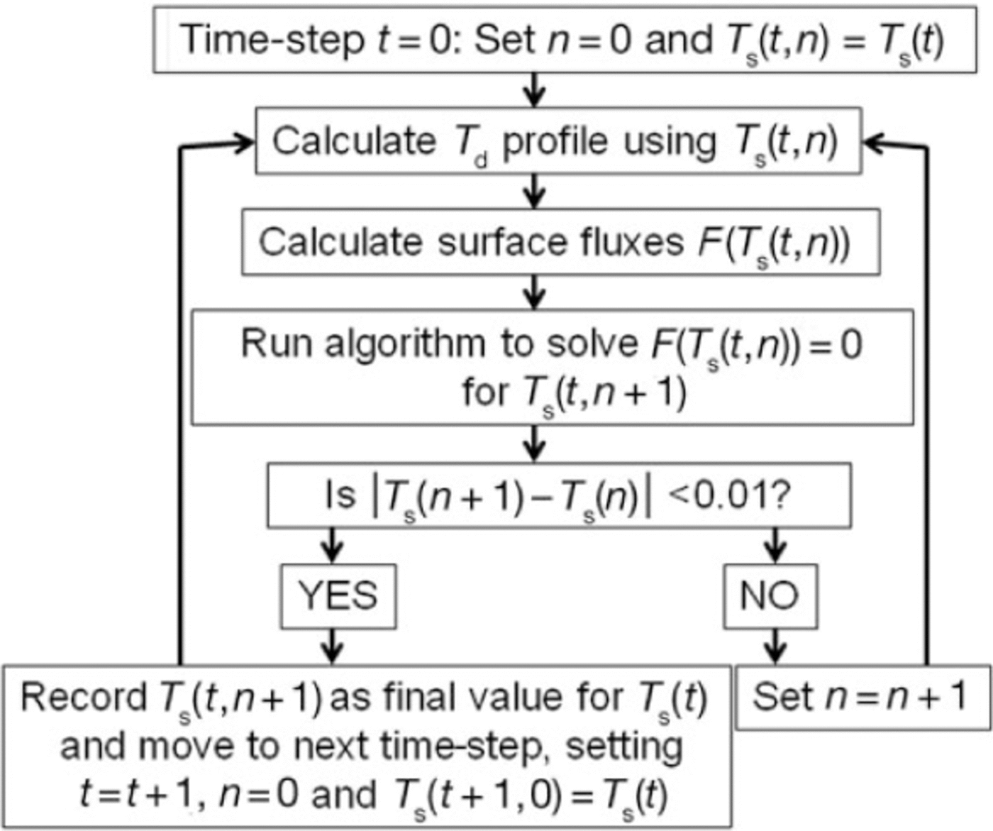
where F’(Ts), the derivative of the total surface flux with respect to T s, is calculated numerically by the central difference method. At each time-step in the model an initial guess of Ts(n = 0) must be made: for the first time-step it is set equal to the air temperature, T a, and thereafter it is set at the value of T s calculated for the previous time-step.Equation (3) is calculated repeatedly until the point where |T s(n + 1) – T s(n)| <0.01.
Debris internal temperatures
Several workers, including Reference Greuell and KonzelmannGreuell and Konzelmann (1994), Reference Koh and JordanKoh and Jordan (1995) and Reference Pellicciotti, Carenzo, Helbing, Rimkus and BurlandoPellicciotti and others (2009) have investigated the influence of subsurface heat conduction into debris-free ice and snow. This flux can be significant when there is a nonzero gradient of temperature with depth, or when some solar shortwave flux penetrates into the snow/ice. The conduction can be calculated from a heat-conservation equation based on Fourier’s law, taking into account the partial derivatives of temperature, T i s, with respect to time, t, and depth, z:

where ρi,s, c i,s and k bs are, respectively, the density, specific heat capacity and thermal conductivity of the ice or snow. For the DEB model, we adapt Equation (4) to apply to a debris layer. The first term on the right-hand side represents heat conduction, while the second term generally accounts for radiative fluxes, Q, penetrating into an ice or snow layer from above. We can assume that no radiative fluxes penetrate rock, and therefore the second term, ∂Q/∂z, can be ignored. The equation is then solved by dividing the debris layer into several calculation layers and applying a numerical algorithm with boundary conditions defined by the surface temperature, T s, and the temperature of the debris base, which is in contact with the glacier ice and is assumed to remain at the melting point of ice, T f = 273.15 K, during the ablation season, as justified by measurements. Generally the number of calculation layers, N, is chosen so the model calculates temperatures at 1 cm intervals, unless the cover is thinner than 5 cm, in which case the number of layers is fixed at 5. This method is fully described in the Appendix, and shows that despite a laborious proof the final algorithm can be applied with only a few lines of code, and is not computationally intensive.
Surface heat fluxes
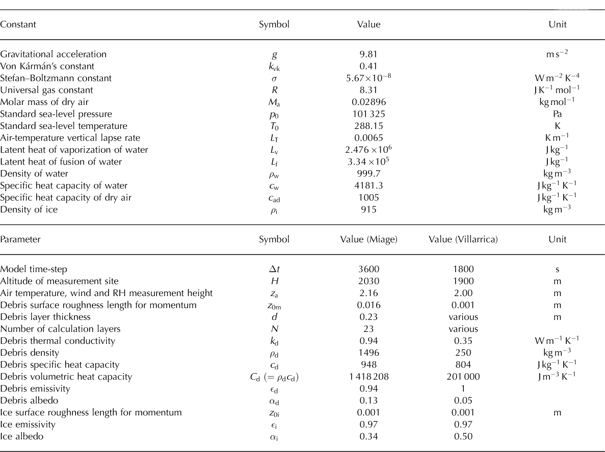
Reference Brock, Mihalcea, Kirkbride, Diolaiuti, Cutler and SmiragliaBrock and others (2010) present equations for the heat fluxes on the surface of Miage glacier that are well justified by reference to existing parameterizations, and assessed for their suitability for a debris-covered surface. In this paper, the same equations are used, with some modifications. We apply the convention that positive fluxes are directed towards the debris surface, and all fluxes are in units of Wm-2. Table 1 displays all the main quantities used in the model, including ‘constants’, which should not change significantly across different sites, and ‘parameters’, which may vary across different sites.
‘Constants’ used in the DEB model, which are well known and should not change significantly across different sites, and ‘parameters’, which may vary across different sites. Default parameter values are given for Miage glacier and Villarrica. All parameter values are based on values given by Brock and others (2007, 2010), unless otherwise stated in the text
Solar shortwave radiation
Incoming (S↓) and reflected (S↑) solar shortwave radiation data were used to compute net shortwave S = S ↓-↑ at the debris surface. Alternatively, one can use S =(1-αd)S↓, where «d is the debris albedo. For future applications in which the shortwave radiation has not been measured, the model could accept inputs from other models that calculate top-of-atmosphere shortwave and incorporate attenuation, diffusion, reflection and shadowing to give a value for the surface shortwave.
Longwave radiation
Downwelling longwave radiation, L↓, is also supplied to the DEB model from data, but as with shortwave radiation it could be simulated in future applications. Upwelling longwave radiation is calculated from the Stefan-Boltzmann law:
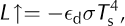
where єd is the debris surface emissivity and σ is the Stefan- Boltzmann constant.
Turbulent heat fluxes
The bulk aerodynamic method was used to calculate turbulent fluxes of sensible and latent heat. First, the stability of the surface layer is assessed by calculating the bulk Richardson number:
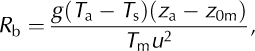
where g is gravitational acceleration, z a is the height of measurement of air temperature, z 0 m is the surface roughness length for momentum and T m is the mean air temperature between the surface and height z a, calculated as T m = (T a + T s)/2. R b is used to calculate nondimensional stability functions for momentum (Φm) heat (Φh) and moisture (Φv). For a stable surface layer, R b ≥ 0:

For an unstable surface layer, R b < 0:

Now, sensible (H) and latent (LE) heat are calculated as
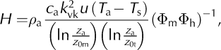
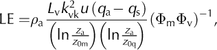
where k vk is von Karman’s constant, L v is the latent heat of vaporization of water, q a and q s are specific humidities at the measurement height, z a, and at the surface, respectively, calculated from relative humidity and temperature data by standard empirical formulae, and z 0t and z 0q are the surface roughness lengths for heat and humidity, respectively, considered equal to z 0m. The specific heat capacity of air, c a, is corrected for a humid atmosphere using the formula c a = c ad(1 + 0.84q), where c ad is the specific heat capacity of dry air. The density of air, ρ a, is calculated according to the ideal gas law:

where R is the universal gas constant and M a is the molar mass of dry air. The air pressure, p a, is estimated based on the altitude, H, of the glacier site:
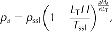
where p ssl and T ssl are the standard pressure and temperature at sea level, and L T is the temperature lapse rate with altitude. We make the intuitive assumption that there can only be a latent heat flux at the debris surface when the surface is saturated (RHs is 100%), implying that there is either surface water to evaporate, or sufficient water vapour to condense. This condition is imposed by setting LE = 0 whenever RHs < 100%.
Heat flux due to precipitation
The heat flux due to precipitation is calculated in a similar manner to Reference Hay and FitzharrisHay and Fitzharris (1988) and A. Bliss (http://escholarship.org/uc/item/8r38754s):

where pw is the density of water, c w is the specific heat capacity of water, w is the rainfall rate in m s-1 and Tr is the rain temperature, which in the absence of complete information is set equal to the measured air temperature, T a. P is often ignored in glacier studies because it tends to be extremely small, but for future studies of glacier retreat under shifting global precipitation regimes it could be an important heat flux, for example on Himalayan glaciers that experience monsoon rains. For this paper, precipitation data are not available for the exact glacier sites, but we make use of data from the nearby Lex Blanche station. The effects of precipitation could be more accurately modelled using rain- gauge and lysimeter data to calculate how much rain evaporates from the debris, and how much percolates through the debris layer to supply a heat flux to the ice (Reference Sakai, Fujita and KubotaSakai and others, 2004). This could potentially improve the accuracy of the DEB model’s latent heat, precipitation heat flux and internal temperature calculations. However, given the absence of the necessary data, this is left as a project for future work. Our approach considers only the effect of precipitation heat flux at the top of the debris layer, where the surface energy balance (Equation (1)) is defined.
Conductive heat flux
The conductive heat flux, G, at the debris surface is calculated based on the temperature gradient at the top of the debris layer, approximated using the surface temperature, T s, and the temperature, T d(1), at the first calculation layer for debris:

where h is the thickness of each calculation layer (usually set to 1 cm) and k d is the thermal conductivity of the debris.
Calculating glacier melt
The only heat flux considered to reach the glacier ice is a conductive flux, G i, which depends on the temperature gradient at the base of the debris:

The ice melt (m w. e.) for the time-step, assuming no further downward conduction of heat, can then be calculated as:
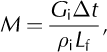
where Δt is the model time-step, p is the density of ice and Lf is the latent heat of fusion of water. A caveat is built in, so that, if the melt rate is calculated to be negative (due to negative temperatures in the debris layer above), it is set to zero; thus, the DEB model implicitly assumes there is no accumulation in the ablation zone because all meltwater runs off immediately without pooling and refreezing.
Overall model structure
The run structure of the DEB model is dominated by the Newton-Raphson iteration procedure for solving surface temperature. It is summarized in Figure 2.
Flow chart illustrating the DEB model run progression, centred around the Newton_Raphson algorithm for calculating surface temperature.
Bare-ice model
To quantify the effects of debris on ablation, a bare-ice melt model was developed for comparison with the DEB model. It includes the assumptions that the ice surface remains at T s = 0°C and can be considered saturated for the purposes of latent heat calculations. Melt rate (mw.e.) for the time- step is calculated from the total sum of heat fluxes:

where αi, is the ice albedo, and all the heat fluxes are calculated using the same equations described above, but with emissivity and surface roughness lengths corrected for ice instead of debris (see Table 1). The downwards conductive flux, G, is considered negligible.
Results and Discussion
Unless otherwise stated, the r 2 values presented in this section represent the Nash-Sutcliffe model efficiency coefficient, and refer to the fit between modelled and measured surface temperature, T s.
Fully mechanistic model
The DEB model can be considered mechanistic at this stage, since all the processes and quantities involved are informed by empirical equations and field measurements as far as possible; none have been adjusted to fit a dataset. Also, all the variables were measured at one site and have not been extrapolated to other areas. As can be seen in Figure 3a, the default parameter values in Table 1 are sufficient for the model to produce surface temperature values with a very good fit (r2 = 0.9437) to the data across the whole 2005 ablation season. Similar fits were acquired for 2006 (r2 = 0.9469) and 2007 (r2 = 0.9421).
Model outputs for the Miage glacier AWS site (2030ma.s.l.) using the default parameter values listed in Table 1. (a) Modelled and measured debris surface temperature, (b) debris internal temperature at 15 cm depth and (c) modelled hourly melt rate for the 2005 ablation season. (d, e) Mean daily cycles of modelled and measured debris surface temperature (d) and surface heat fluxes (e), for the ablation seasons of 2005, 2006 and 2007.

Figure 4a shows the mean daily cycle of modelled debris temperatures across the 2005 ablation season. There is an obvious lag with depth, so the maximum temperature at the bottom of the layer occurs ˜3-4 hours after the maximum surface temperature. This is to be expected since heat conduction through the debris will take some time, and it concurs with Reference Nicholson and BennNicholson and Benn (2006), who reported lags of 3-4 hours between the surface temperature and 20 cm depth in a debris layer on Ngozumpa Glacier, Nepal. Figure 4b illustrates this lag in more detail: there are nonlinear temperature profiles when the layer is warming or cooling, but approximately linear profiles at the warmest (1500 h) and coldest (0600 h) times of day.
Modelled debris temperature during the ablation season on Miage glacier in 2005. (a) Average value for every hour of the day and (b) line plots for selected times of day.

However, a discrepancy arises when the modelled temperature is compared to data. Figure 3b shows the modelled debris temperature at 15 cm depth alongside measured data for the same depth, which were collected using thermistors at a separate site near the AWS between 0100 h on 21 June and 1900 h on 24 July. The modelled mean (4.4°C) and measured mean (4.1 °C) temperatures are very similar, but the overall fit is poor (r2 = 0.5173) because the modelled temperature lags behind the data by ˜3 hours. This lag is not a function of the model’s numerical procedures and finite time-step, since the lag remains the same even when data are interpolated to run the model with a much shorter (1 min) time-step. The lag may arise due to varying debris properties that affect thermal diffusivity at the two sites, such as the prevalence and connectivity of void spaces which could affect non-conductive processes such as windpumping (Reference HumlumHumlum, 1997). Alternatively, there may be an error in the measured 15 cm temperature due to direct solar heating of the thermistor cables that were lying on the debris surface: conduction down the cables could cause temperatures to rise too quickly in the morning. These are areas that should be investigated using more accurate measurements of the debris thermal profile. In the meantime, any lag-induced error in temperature gradient at the debris base, which determines melt, will be very small and should even out over time, meaning that the main quantities of interest (mean daily or seasonal melt rates) should be unaffected. Figure 3c displays the modelled hourly melt rate in mm w.e. h-1 and, as might be expected, the melt rate follows a similar trend to surface temperature (Fig. 3a). The calculated mean daily melt rates, M day, were 14.5, 15.4 and 13.7 mm w.e. d-1 over the ablation seasons of 2005, 2006 and 2007, respectively. Figure 3d shows mean daily cycles of temperature and surface heat fluxes for 2005, 2006 and 2007, and Table 2 presents the mean, maximum and minimum of these cycles. In all three years the mean modelled surface temperatures are higher than the data by just over 1 °C. There are many reasons why this could occur, but one physical interpretation is that the data were calculated from radiative measurements of upwelling longwave; this required a value for surface emissivity, which may have been overestimated.
Mean, daily maximum and daily minimum debris surface temperatures on Miage glacier (°C) as measured (data) and as calculated by the DEB model, for 2005, 2006 and 2007
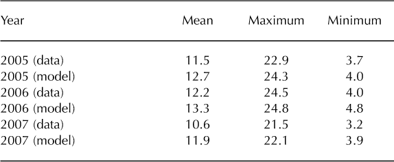
Figure 3e shows the mean daily cycles of surface heat fluxes. The mean latent heat flux (LE) values were calculated for 2005 and 2007 using only those data points where surface RH data were available, and there is no latent heat flux for 2006 due to lack of data. The wettest year was 2007, with considerable evaporation, as reflected in the relatively large negative latent heat flux and lower surface temperature.
Sensitivity analysis
Arguably, the parameters with greatest uncertainty in the model are the physical properties of the debris layer: ∊d, z 0m, k d, p d and c d. In particular, the model in its current form makes the assumption that k d, p d and c d are constant with depth, which is undoubtedly not the case in the real world. Debris layers tend to have an inhomogeneous structure, with dry rubble and boulders on top containing considerable air spaces, and smaller rubble and fine particles beneath, which may often be saturated with water near the glacier ice. A more advanced model could account for this variation by allowing physical properties to vary with depth; however, a verification of the model would require detailed data on internal debris temperature and water content, and is beyond the scope of this paper. Instead, the parameters are investigated via a standard sensitivity analysis. Table 3 illustrates how the model’s r 2 fit to surface temperature, and the mean daily melt rate, M day, on Miage glacier in 2005 respond to changes in the debris properties. Each parameter is varied from its default value by ±10%, except for ∊d, because it does not make physical sense to increase it above 1. Also, because p d and c d are always multiplied together in the model, they are considered as one parameter, C d = p d c d, the volumetric heat capacity. It should be noted that this analysis is very specific to the 2005 season on Miage glacier;and given that the parameters almost certainly influence each other in ways that are difficult to quantify, it would not make physical sense to change any one parameter dramatically without changing the others. Therefore the changes in each parameter are kept relatively low (up to 10%). This reflects our aim to be entirely mechanistic wherever possible; the analysis is more a tool for deciding which parameters are important and could therefore benefit from more accurate estimates in the field.
Response of r 2 and M day upon changing parameter values, for the 2005 ablation season on Miage glacier
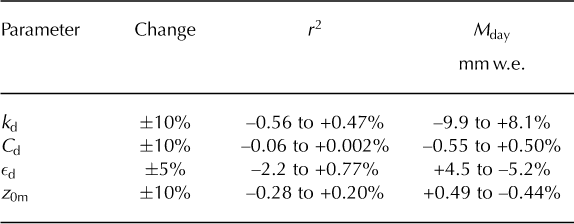
The model fit and melt rate are relatively insensitive to C d and z 0m. The fit improves slightly upon increasing e d, accompanied by a small decrease in melt rate due to greater longwave emission from the surface. A ± 10% change in k d produces up to a 10% change in melt rate. This highlights the importance of k d in the debris energy balance. However, although the average k d for a debris layer can be estimated by observing melt rates (Reference Brock, Mihalcea, Kirkbride, Diolaiuti, Cutler and SmiragliaBrock and others, 2010), it is hard to quantify how it may vary with depth; solid rock tends to have kd values ˜2-7Wm-1 K-1, while the air spaces in between have a much lower k d, ˜-0.025Wm-1 K-1. The heat transfer in the upper debris may be dominated more by turbulent processes than conduction, and water at the base of the debris, with thermal conductivity ˜0.58Wm-1 K-1, will add further complicating effects. These phenomena should be a focus of future studies.
Significance of variables
The good fit to data provided when running the model with default parameter values provides a strong indication that all the physical theory implemented in the model is sound. However, it is useful for both model parsimony and scientific insight to test whether individual components of the model are entirely necessary for a strong fit. In this case, the components of most interest are the individual heat fluxes. The importance of each flux was assessed by removing the equations for calculating the flux (setting the flux to zero) and calculating the new fit of the model. Based on the results in Table 4, the shortwave, longwave, conductive and sensible heat flux equations are clearly essential for the model to perform well, because the model r 2 fit to surface temperature suffers significantly when any of them are removed. The results also suggest that latent heat, LE, produces a smaller, though still significant, improvement in fit for the periods in which it was calculated.
Response of the DEB model’s fit to surface temperature data, r2, and mean daily melt rate, Mday (mm w.e.), when individual heat fluxes were set to zero. All are significant changes in fit to the 95% confidence level, except that marked with an asterisk. For latent heat flux, LE, the fit refers only to those times when surface RH was measured (1702 data points in 2005, 533 in 2007)
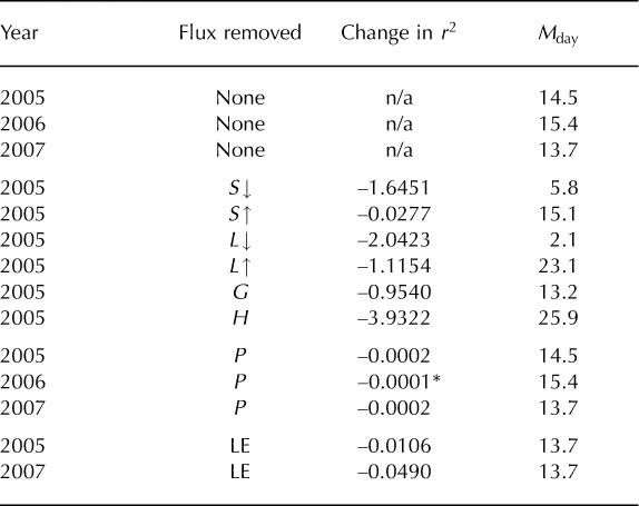
The change in r 2 on removing the heat flux from precipitation, P, from the model is tiny. Even so, it is deemed significant in 2005 and 2007, but not 2006 (assessed by performing statistical F-tests on the ‘improvement’ in fit incurred by including the flux). This suggests that P may have a significant effect on the glacier surface energy balance. However, such results should be treated with caution; it is difficult to define the degrees of freedom in a nonlinear model which uses each variable multiple times and has no parameters adjusted to fit, and the F-test will tend to place undue significance on even tiny improvements in fit for such a large dataset. There is also a considerable unquantifiable error caused by using precipitation data from Lex Blanche, 4 km from the glacier. For these reasons, and given that the model provides a very significant fit without P, precipitation data are deemed unnecessary for applying our model to debris-covered alpine glaciers in its current form, but it is certainly an area for further study. The heat flux from precipitation could become more significant in areas of heavy rainfall, such as monsoon regimes in the Himalaya, and build-up of rainwater within debris could have strong effects on heat conduction. Therefore precipitation measurements could form a valuable part of future fieldwork on debris-covered glaciers. Similar F-tests were used to assess whether the variability in each input variable was essential for a good fit to surface temperature, for purposes of simplifying the model. Table 5 presents the change in model fit when each variable was set to its mean value for the whole ablation season, thus removing its variability – an approach inspired by the ‘model reduction’ techniques described by Reference Cox, Gibbons, Wood, Craigon, Ramsden and CroutCox and others (2006) and Reference Crout, Wood and TarsitanoCrout and others (2009). This shows that w, the precipitation data from Lex Blanche, either gives no significant improvement in fit, or actually makes the fit worse (r2 increases when it is removed, implying that the precipitation data add unnecessary noise to the model). More interestingly, the same can be said about RHa, the relative humidity in air measurements made at the Miage study site. This implies that the improved fit provided by adding the heat flux from precipitation, P, and latent heat, LE, to the model, as reported above, arises solely from the other variables and parameters included in the equations.
Change in model fit, r2, on setting each input variable in turn to its mean value for the whole ablation season. All are significant changes in fit to the 95% confidence level, except those marked with asterisks. RHs was not measured in 2006
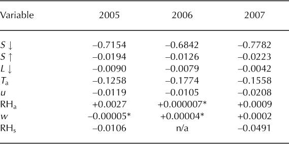
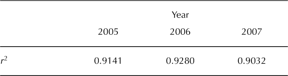
Table 5 also shows that the improvements in fit on including variability in upwelling shortwave radiation, S↑, downwelling longwave radiation, L↓, wind speed, u, and surface relative humidity, RHs, are very small. These results indicate that the melt rates of debris-covered glaciers in the Alps could be modelled to a reasonable degree of accuracy using only shortwave radiation and air-temperature data, as has been noted for clean glaciers in the Alps (Reference Pellicciotti, Brock, Burlando, Strasser, Funk and CorripioPellicciotti and others, 2005). This was tested by setting all variables except S↓ and T a to their mean values for the ablation season, and Table 6 shows that the model still provides a strong fit to surface temperature data (r2 > 0.9) for all three years. This is encouraging for developing simpler models of melt rates on such glaciers. However, more work is required to determine whether the same simplifying assumptions could be made for glaciers in other mountain ranges. In any case, the debris layer thickness and thermal properties have a huge effect on melt rates and should be included in any model if it is to be generalized to areas where these properties are different. Remote-sensing approaches to mapping debris thickness (e.g. Reference MihalceaMihalcea and others, 2008) could provide the necessary inputs to such models.
Model fit to surface temperature data when the only variability in the model comes from solar shortwave radiation and air-temperature data.
It should be noted that the removal of RHs variability from the model amounts to completely removing the latent heat flux, LE, due to the way the model is formulated. This results in a moderate but significant reduction in r2, implying that the variability in RHs improves the model. An accurate calculation of latent heat flux by bulk-transfer theory will always require data on surface humidity, but RHs is generally not measured on or near glacier sites, or predicted by global or regional-scale climate models. We conclude that although latent heat flux is of secondary importance for useful energy-balance models of alpine glaciers, supporting the findings of Reference LangLang (1981) for clean glaciers, there remains a challenge for future field and modelling studies to parameterize it without such requirements on surface data, especially for other areas of the world, where latent heat fluxes may become more significant.
Cross-validation
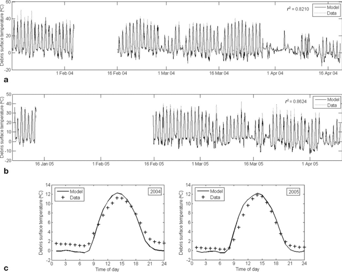
To determine whether the DEB model could be generalized to other glacier systems, it was tested using data collected on the tephra-covered glacier of Villarrica volcano in 2004 and 2005 (described by Reference Brock, Rivera, Casassa, Bown and AcunaBrock and others, 2007). Data were collected half-hourly according to a regime similar to that on Miage glacier, but given a lack of surface RH and precipitation data it was not possible to calculate latent heat flux, LE, or the flux from precipitation, P. Furthermore, given the uneven spread of tephra compared to the debris cover on Miage glacier, the surface temperatures were not measured directly beside the AWS, but on tephra banks up to 100 m away. These sites had tephra thicknesses of d = 0.32 m in 2004 and d = 0.13 m in 2005. It should also be noted that the surface temperature was measured using thermistors which experience greater errors than the radiative temperature measurements used at Miage glacier, due to occasional exposure to direct solar heating or wind cooling. The default parameter values for Villarrica are shown in Table 1. Figure 5 shows the surface temperatures calculated using the DEB model for 2004 and 2005, which provide a good fit to data in both years, especially considering that the input data were measured at a different site to the surface temperature. However, as Figure 5c and d show, the model consistently underestimated night-time surface temperatures by as much as 2°C. This can be explained by noting that air temperature on Villarrica dropped below 0°C on several occasions during measurement. This means that the assumption in the DEB model, that the debris/ice interface remains at 0°C, may not be suitable; in fact the interface temperature probably goes below 0°C. The DEB model compensates for this incorrect assumption by setting Ts lower than it should be. Similar problems were found by Reference Nicholson and BennNicholson and Benn (2006) for melt models at Larsbreen, Svalbard; they argue that these colder regions may require models to include conductive heat fluxes into the ice. Further work is required to make the DEB model capable of calculating accurate debris temperatures for this situation, given that some energy is required to heat up the ice and debris before melting can take place again.
Model outputs for Villarrica glacier using the default parameter values listed in Table 1. Modelled and measured debris surface temperature in (a) 2004 and (b) 2005, and mean daily cycles of surface temperature in (c) 2004 and (d) 2005.
Effects of debris thickness
Perhaps the most interesting and useful application of the DEB model is that it can be used to estimate mean daily melt rates as a function of debris thickness. The curve in Figure 6a shows the results of several model runs for Miage glacier in 2005 using varying values of debris thickness, d, plotted with data collected at several sites on the glacier. No goodness of fit is calculated for Figure 6a because, although the model is run with meteorological inputs from the AWS site, the data points represent sites at a variety of other positions on the glacier, where variations in altitude, aspect and shadowing result in very different meteorological conditions. In particular, data from the upper glacier (where the glacier turns north, elevation increases more sharply and the glacier experiences greater shadowing effects from the Mont Blanc massif) are shown with different markers to indicate that they should not be directly compared to the model curve. Despite this limitation, the DEB model matches the data well, not only at the AWS site (indicated) but also at higher debris thicknesses up to 55 cm. However, it overestimates the melt rate for debris layers thinner than ˜-14cm. This is partly because most of the thin-debris measurements were taken at higher parts of the glacier, but may be further explained by an observed positive relationship between k d and d (Reference Brock, Mihalcea, Kirkbride, Diolaiuti, Cutler and SmiragliaBrock and others, 2010). The bare-ice model predicts a higher melt rate than was measured (71 vs 58mmw.e. d-1), but again it should be noted that the bare-ice measurements were made some distance up-glacier from the AWS. Furthermore, the colder surfaces presented by thinner debris layers and bare ice during the ablation season are likely to reduce air temperatures relative to a 23 cm layer, and the atmospheric boundary layer may have a very different structure, with the surface becoming a sink for sensible heat rather than a source. Such discrepancies could be partly taken into account in distributed models by applying suitable lapse rates, dependent on altitude and debris patterns.
Modelled and observed mean daily melt rates plotted against debris thickness, for (a) Miage glacier and (b) Villarrica glacier. Note that the data used to run the DEB model for Miage glacier (a) were recorded at an AWS (indicated data point) on the lower glacier. Melt data from the upper glacier, where meteorological conditions are quite different, are shown separately because they should not be directly compared to the curve.
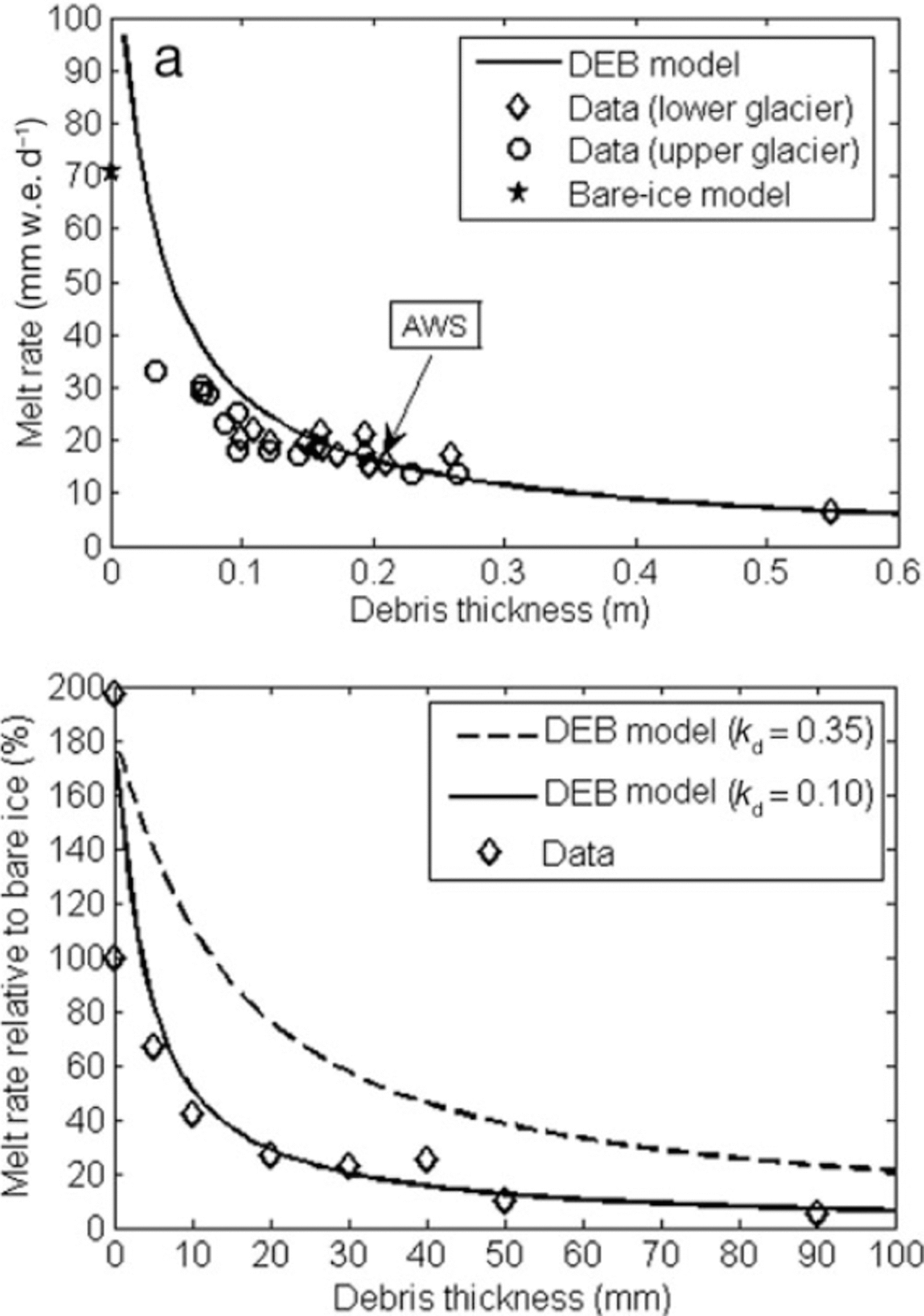
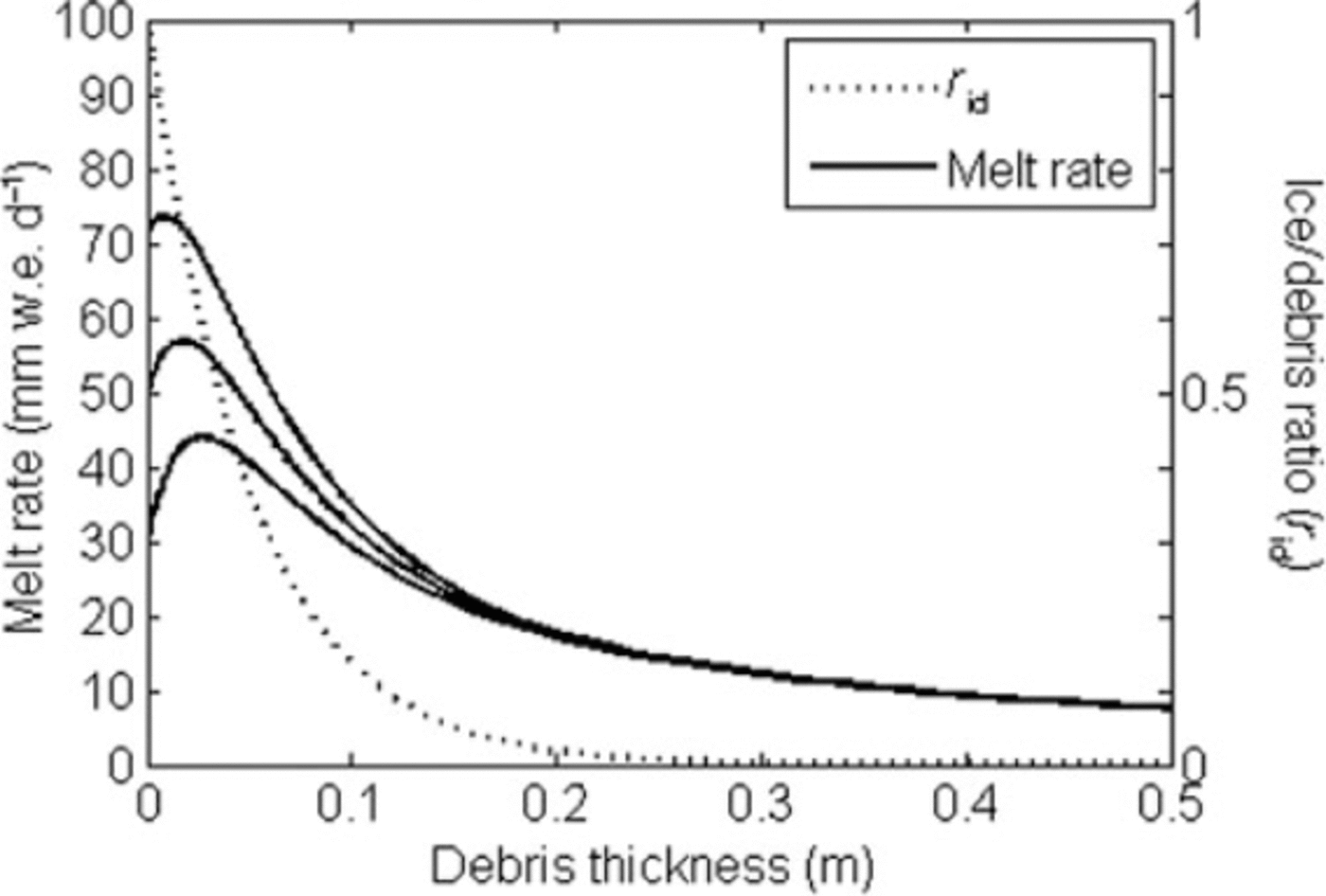
Figure 6b shows similar predictions for Villarrica glacier, using a 6 day block of meteorological data from January 2005. The model predictions are plotted with data recorded around the same time during an experiment in which ablation was measured on artificial plots with various debris thicknesses. The sub-debris melt rates are shown relative to bare-ice melt rates to account for differences between the experiment site and the AWS site. As can be seen, the melt rate is very sensitive to thermal conductivity;with the default value of kd = 0.35, the model overestimates the melt rate, while using a value of k d = 0.10 provides a good match to the data. This may be because the default value of 0.35 was calculated from measurements in 2004 on thicker, natural debris layers (11-32 cm);these were subjected to compression under a winter snowpack, and may even have been reexposed after previous incorporation inside the glacier ice. Conversely, the artificial tephra covers created to collect the data in Figure 6b had looser, lighter structures with more air pockets, meaning they would undoubtedly show lower thermal conductivity than the compact layer. In any case, this result highlights the importance of debris thermal conductivity as a parameter to consider in any study of a debris-covered glacier. Interestingly, the DEB model predicts that very thin debris layers will produce a melt rate higher than the bare-ice melt rate. This enhancement was not seen in the Miage glacier melt data, but a large melt enhancement, of 197%, was observed for a very thin dusting of tephra (estimated by Reference Brock, Rivera, Casassa, Bown and AcunaBrock and others, 2007, to have thickness 0.25 mm) on one of the Villarrica experimental plots (the upper data point close to the y-axis in Figure 6b). This finding can be related to a well-established feature of debris-covered glaciers, the ‘0strem curve’ (0strem 1959), which shows that very thin debris covers increase ablation rates by darkening the surface, while debris covers thicker than a certain ‘critical thickness’ reduce ablation. The critical thickness has been shown to vary considerably across glaciers in different locations and with different types of debris cover (Reference Kirkbride and DugmoreKirkbride and Dugmore, 2003). As Figure 6 shows, the melt rate certainly increases for thin debris layers, but there is no sign that it reaches a maximum and then decreases towards the bare-ice melt rate as the debris thickness tends towards zero. In reality, a smooth 0strem curve may arise for reasons that are not incorporated in the DEB model. For example, the transfer of heat is not restricted to the vertical dimension, and the melt rate at one point will be affected by its immediate surroundings. In particular, one can observe that thin debris layers tend to be more sparsely scattered than thicker layers, exposing more high-albedo areas of ice that may reduce the melt rate. For debris layers made of dust or small particles, the situation may be more complicated, as shown by Reference Adhikary, Yamaguchi and OgawaAdhikary and others (2002), who demonstrated that a uniform dust layer on snow begins to aggregate as the snow melts, thus reducing the ablation rate. On Miage glacier, where the scattered debris cover may vary from sand-sized particles to huge boulders, the situation can be approximated by defining a ‘patchiness’ parameter, r id, representing the ratio of exposed ice to debris-covered ice. The melt rate can then be calculated as:

where M bare is the melt rate for bare ice, and M debris is the melt rate under a debris layer. r id was defined by an exponential decay dependence on the debris thickness, d, simulating the fact that as the debris layer thickens, less ice will be exposed:
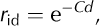
where C is a constant. Figure 7 shows the melt rates calculated in this manner for Miage glacier in 2005, with C = 20 (note that this value is not based on observations, and is chosen arbitrarily for the purposes of our ‘thought experiment’). The top curve uses the bare-ice melt rate calculated by our model (= 71 mmw.e. d-1), and the other two use bare-ice melt rates of 50 and 30mmw.e.d-1, to show that the effect is enhanced when the thin-debris melt rate is significantly higher than the bare-ice melt rate. The lines closely resemble 0strem curves. This suggests an interesting proposition for future field studies: quantifying r id for various types and thicknesses of debris layers, and thus how it affects glacier melt rates
Melt rates (solid curves) over a scattered debris cover, calculated using the DEB model and a bare-ice model with Miage glacier data. The ratio of exposed ice to debris-covered ice, rid, is represented by the dotted curve (note that this curve is not based on any observed data, and is chosen arbitrarily for the purposes of this theoretical exercise). The solid curves were calculated by assuming bare-ice melt rates of, from top to bottom, 71 (the bare-ice model prediction), 50 and 30mm w.e.d-1.
Summary and Conclusions
We have presented the DEB model, a detailed energy- balance model for a debris-covered glacier, which centres around an iterative calculation of surface temperature and includes conduction through the debris layer. The fact that this approach accurately reproduces long-term, high-resolution surface temperature data on two very different debris- covered glaciers, without fitting any parameters, is a satisfying indication that the assumptions and physics used to calculate surface heat fluxes are accurate, and the model is generalizable to different systems. The DEB model and the extensive dataset from Miage glacier allow a thorough statistical analysis of different aspects of energy balance at a debris surface, which helps to justify some assumptions that have been made in previous energy-balance models;for example, it indicates that the heat flux from precipitation is negligible for alpine glaciers, and that latent heat can be omitted without large losses in model performance. The main advantage of the DEB model is that it calculates the ice melt rate beneath supraglacial debris directly from meteorological data, without the need for surface temperature measurements. Hence, it can be applied to most of the world’s debris-covered glaciers, since meteorological data are likely to be available, even if these come from a reanalysis program. The main challenge, particularly in glacial modelling at a regional scale, is in acquiring information on the extent, thickness and thermal properties of supraglacial debris covers. Such data could be obtained via remote sensing (e.g. Reference Paul, Huggel and KaabPaul and others, 2004;Reference MihalceaMihalcea and others, 2008) combined with suitable field validation (e.g. Reference Brock, Mihalcea, Kirkbride, Diolaiuti, Cutler and SmiragliaBrock and others, 2010). The DEB model could also be used to assess future meltwater production from debris-covered glaciers using climate-model outputs, but such an approach would require understanding of potential changes in supraglacial thickness and extent over time; processes which are currently poorly understood. The DEB model is a very detailed approach to glacier-melt prediction, and is probably more complicated than a melt model needs to be for most practical applications (e.g. as a component in large- scale hydrological catchment models). As has been shown, not all the simulated processes are essential for good model performance in both the Alps and the Andes, since model efficiency is dominated by just two input variables: air temperature and incoming shortwave radiation. It would be useful to develop a family of simpler, empirical models based around the same variables as the DEB model, and compare them on a thorough statistical basis using model- selection criteria (e.g. Reference Cox, Gibbons, Wood, Craigon, Ramsden and CroutCox and others, 2006). In the interests of pure science and understanding of glacier thermodynamics, the DEB model presents a useful platform for investigating even more detailed processes within a debris- covered glacier (e.g. variations in structure, moisture, and hence thermal properties, with depth in the debris layer). For application to colder regions, the model should include downwards conduction into ice, which would decrease melt slightly at times when the ice acts as a heat sink (Pellicciotti and others, 2010). Finally, in the context of large-scale distributed models, the DEB model should be easy to combine with existing models for debris-free ice and snow, but may require more development if the distributed models were to include the effects of meltwater pooling and refreezing, or bare-ice slopes and cliffs that could present isolated areas of high melt rates (Reference Sakai, Nakawo and FujitaSakai and others, 1998; Reference Purdie and FitzharrisPurdie and Fitzharris, 1999).
Acknowledgements
T. Reid is funded under the EU/FP7 ACQWA (Assessing Climate impacts on the Quantity and quality of WAter) project. Data from Lex Blanche meteorological station were kindly supplied by Regione Valle d’Aosta. We thank R. Essery for useful discussions on modelling 0strem curves and two anonymous reviewers for comments on the manuscript.
Appendix
Software
The DEB model is implemented in MATLAB® Release 2009b, copyright 1984-2009, The Mathworks, Inc. All model code is available on request from the authors.
Notes on the Newton-Raphson iteration method
The Newton-Raphson algorithm, as described in Equation (3), performs well for calculating T s, but is occasionally unstable due to large step sizes calculated when F’(Ts(n)) is very small. To avoid these instabilities, a maximum step size of | T s(n + 1) — T s(n)| ≤ 1 °C is imposed at each stage of the algorithm. On some other occasions, the algorithm gets stuck jumping between two values on either side of a function minimum. To deal with this situation, the algorithm is always stopped if the number of steps, n, reaches 100 and the mean of the last two values is taken as the true solution for T s.
Calculating internal debris temperatures
The heat conservation equation for the debris layer is informed by Equation (4), and takes into account the partial derivatives of debris temperature, T, with respect to time, t, and depth, z, in the form

where ρ, c and k are the debris density, specific heat capacity and thermal conductivity, respectively (the subscript'd' for debris is not used in this Appendix, for clarity). For a debris layer of thickness d, we define N internal calculation layers, each with thickness h =d/N, such that the jth layer is at depth z j = jh (j = 0, 1, 2,…, N). Similarly, for a time-step of size Δt, the mth time-step is at t m = mΔt (m = 0, 1, 2,…). Now, to calculate temperature in the jth layer at time m + 1, we can integrate Equation (A1) over the intervals [z j -12, z j+12] and [tm , t m+1]. By adopting the notation Tj m for the debris temperature at time-step m in layer j, the left-hand side of Equation (A1) becomes:

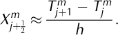
Next, we define the function X(z, t) = ∂T/∂z, which is calculated at a depth of z j+12 by applying the central difference approximation:
Now the right-hand side of Equation (A1) can be rewritten as:
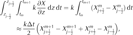
where the time integration on the last step is solved using a trapezoidal approximation, which is sufficiently accurate for a short time-step. Finally, by combining Equations (A2) and (A4), and expanding all terms in X according to Equation (A3), we obtain the numerical scheme
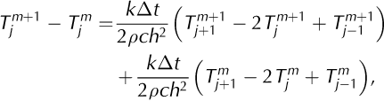
which shows that the change in temperature of layer j from one time-step to the next depends on temperatures in layer j and its neighbouring layers, j — 1 and j + 1, at both the new (t m+1) and previous (tm ) time-steps. Equation (A5) represents a series of equations that can be written out in the Crank- Nicholson form, here using the notation of Reference SmithSmith (1985), with everything known on the right-hand side and everything unknown on the left:
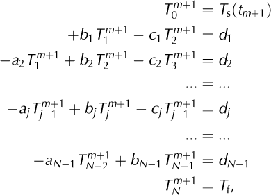
where the as, bs, cs and ds are all known quantities. The top and bottom equations contain two boundary conditions for the scheme: the newly estimated debris surface temperature Ts(tm+1 ) and the temperature of the debris base, which is assumed to remain at the freezing point of water, T f = 273.15 K. Defining a constant C = kΔt/2ρch2, Equation (A5) can similarly be rewritten with known quantities on the right and unknowns on the left:

Comparing Equations (A6) and (A7), we infer that the required constants are
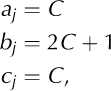
for all, where = 1, …, N – 1. The values of d are:
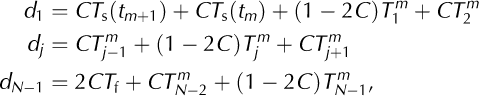
where the second equation applies to j = 2,…, N - 2. Continuing in the notation of Reference SmithSmith (1985), we define two variables A and S:


where i- 2,N - 1. Finally, the debris temperature at each internal layer in the ice for the new time, f m+1, can be
calculated using:
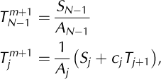
where the calculations for the second equation must be done in reverse order, j – N - 2, N – 1, …, 2, 1. Therefore all that is required to solve the internal debris temperature within the model is to evaluate Equations (A8-A12) in order.



